the Creative Commons Attribution 4.0 License.
the Creative Commons Attribution 4.0 License.
 | 06 Jul 2018
A climatological view of the vertical stratification of RH, O3 and CO within the PBL and at the interface with free troposphere as seen by IAGOS aircraft and ozonesondes at northern mid-latitudes over 1994–2016
Bastien Sauvage
Herman G. J. Smit
François Gheusi
Fabienne Lohou
Romain Blot
Hannah Clark
Gilles Athier
Damien Boulanger
Jean-Marc Cousin
Philippe Nedelec
Patrick Neis
Susanne Rohs
Valérie Thouret
This paper investigates in an innovative way the climatological vertical stratification of relative humidity (RH), ozone (O3) and carbon monoxide (CO) mixing ratios within the planetary boundary layer (PBL) and at the interface with the free troposphere (FT). The climatology includes all vertical profiles available at northern mid-latitudes over the period 1994–2016 in both the IAGOS (In-service Aircraft for a Global Observing System) and WOUDC (World Ozone and Ultraviolet Radiation Data Centre) databases, which represents more than 90 000 vertical profiles. For all individual profiles, apart from the specific case of surface-based temperature inversions (SBIs), the PBL height is estimated following the elevated temperature inversion (EI) method. Several features of both SBIs and EIs are analysed, including their diurnal and seasonal variations. Based on these PBL height estimates (denoted h), the novel approach introduced in this paper consists of building a so-called PBL-referenced vertical distribution of O3, CO and RH by averaging all individual profiles beforehand expressed as a function of z∕h rather than z (with z the altitude). Using this vertical coordinate system allows us to highlight the features existing at the PBL–FT interface that would have been smoothed otherwise.
Results demonstrate that the frequently assumed well-mixed PBL remains an exception for both chemical species. Within the PBL, CO profiles are characterized by a mean vertical stratification (here defined as the standard deviation of the CO profile between the surface and the PBL top, normalized by the mean) of 11 %, with moderate seasonal and diurnal variations. A higher vertical stratification is observed for O3 mixing ratios (18 %), with stronger seasonal and diurnal variability (from ∼ 10 % in spring–summer midday–afternoon to ∼ 25 % in winter–fall night). This vertical stratification is distributed heterogeneously in the PBL with stronger vertical gradients observed at both the surface (due to dry deposition and titration by NO for O3 and due to surface emissions for CO) and the PBL–FT interface. These gradients vary with the season from the lowest values in summer to the highest ones in winter. In contrast to CO, the O3 vertical stratification was found to vary with the surface potential temperature following an interesting bell shape with the weakest stratification for both the lowest (typically negative) and highest temperatures, which could be due to much lower O3 dry deposition in the presence of snow.
Therefore, results demonstrate that EIs act as a geophysical interface separating air masses of distinct chemical composition and/or chemical regime. This is further supported by the analysis of the correlation of O3 and CO mixing ratios between the different altitude levels in the PBL and FT (the so-called vertical autocorrelation). Results indeed highlight lower correlations apart from the PBL–FT interface and higher correlations within each of the two atmospheric compartments (PBL and FT).
The mean climatological O3 and CO PBL-referenced profiles analysed in this study are freely available on the IAGOS portal for all seasons and times of day (https://doi.org/10.25326/4).
- Article
(13640 KB) - Full-text XML
-
Supplement
(421 KB) - BibTeX
- EndNote


As the region of the atmosphere where exchanges of momentum, water and trace chemical species occur with the Earth's surface, the planetary boundary layer (PBL) is of fundamental importance for atmospheric studies. The pollutant concentrations at the Earth's surface are intimately linked to their vertical distribution in the entire PBL, which in turn results from a complex interaction between emissions and deposition at the surface, local chemistry, horizontal advection by the wind, vertical turbulent mixing in the PBL and exchanges with the free troposphere (FT). The vertical extent and structure of the PBL is closely linked to turbulence. Within the PBL, turbulence can be generated by the static instability produced by surface heating (that induces thermals of warm air rising or the advection of cold air masses above warm surfaces) or mechanically through the wind shear at the surface or in the vicinity of jets (Stull, 1988). During the development of the daytime convective PBL, air from the FT or the residual layer (RL) is entrained into the PBL, which modifies the budget of the chemical species (the entrainment flux acting as a source or a sink depending on the species, the location and the time of day). The numerous processes interacting in the PBL lead to a highly variable and complex vertical distribution of pollution.
Over the last decades, continuous effort was put into collecting in situ observations in the troposphere, mainly with commercial and/or research aircraft and sondes and to a lesser extent with instrumented mats and tethered balloons. However, the amount of in situ data available at altitude remains relatively low compared to the surface (both in terms of the quantity of data and number of species). In particular, profiles throughout the entire PBL (i.e. starting from the surface and extending to the free troposphere) are relatively sparse. This limits our ability to properly describe and understand how pollution is vertically distributed within the PBL. One consequence is the difficulty of many state-of-the-art models to accurately reproduce the vertical stratification of pollution. Although some high-resolution chemistry–climate models (CCMs) with interactive stratospheric and tropospheric chemistry can show encouraging results at the episodic scale (e.g. Lin et al., 2012, 2015), several initiatives of models inter-comparison exhibited large errors on the ozone (O3) and carbon monoxide (CO) vertical distribution over longer periods of time (Elguindi et al., 2010; Solazzo et al., 2013). More recently, Travis et al. (2017) highlighted the difficulty of the GEOS-Chem chemistry–transport models (CTMs) to reproduce sharp O3 vertical gradients in the first kilometre above the surface of the south-eastern United States (during both clear-sky and low-cloud conditions), attributed to excessive top-down mixing in the model. Thorough knowledge of the vertical distribution of pollutants within the PBL and at the interface with the FT is required for conducting diagnostic evaluations of CTMs through the entire PBL compartment, and not only at the surface. However, a common difficulty in the evaluation of models is the fact that several error sources may compensate for each other and therefore hide specific model deficiencies. Such error compensations are often complex to identify. In particular, although closely linked, both PBL heights and pollutant concentrations (at the surface and/or along vertical profiles in the PBL) are often evaluated separately, which limits the significance of the drawn conclusions. For instance, a model may reproduce the concentrations of a specific chemical compound well at the surface but overestimate the PBL height and/or the vertical mixing; in this case, this would suggest that its sources are actually overestimated. A recent diagnostic evaluation of the WRF-Chem model focusing (for the first time) on the O3 entrainment highlighted deficiencies in the model, including an overestimation of the O3 entrainment and a too-efficient vertical mixing in the lower PBL (Kaser et al., 2017). These deficiencies were found to originate mainly from errors in the entrainment rate and PBL height during the morning and an erroneous representation of the O3 gradient at the PBL–FT interface during the rest of the day.
Table 1Information relative to the measurements of the parameters used in this study (instrument, uncertainty and period of available data).
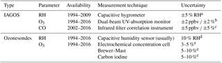
a Helten et al. (1998); Neis et al. (2015a, b). b Thouret et al. (1998). c Nédélec et al. (2015). d Schröder et al. (2017). e WMO (2011).
The general objective of this study is to derive a climatological vertical distribution of O3 and CO over the period 1994–2016 combined with information on the PBL. This paper focuses on these two pollutants, but some results will also be (more briefly) discussed for relative humidity (RH) and potential temperature (θ). For this purpose, we benefit from the two main sources of in situ vertical profiles in the troposphere: (i) the In-service Aircraft for a Global Observing System (IAGOS) database and (ii) the World Ozone and Ultraviolet Radiation Data Centre (WOUDC) ozonesondes database. We first implement an algorithm for automatic estimation of the PBL height from both sonde and airborne profiles. Based on these estimates of PBL height, we derive a climatological description of the vertical stratification of O3, CO, RH and θ within the PBL and at the interface with the FT. Many studies have already provided climatological vertical profiles of O3 and CO, but most of the time simply by averaging individual profiles regardless of whether the PBL height varies. The novel approach developed here consists of providing climatological vertical profiles in a vertical coordinate system based on the PBL height (hereafter referred to as PBL-referenced vertical profiles); the altitudinal dimension of vertical profiles is first normalized by the PBL height, and then profiles are averaged to provide a climatological vertical distribution. While commonly used in studies dealing with PBL dynamics (e.g. Lilly, 2002), to our knowledge this approach has not yet been used to derive climatological vertical profiles of chemical compounds. The main benefit of this approach is to highlight possible specific features in the vertical distribution that would be smoothed with a simple average, in particular at the PBL–FT interface. An illustration is given later in the text.
Data and methods for estimating PBL heights are described in Sect. 2. The climatological PBL heights are analysed in Sect. 3, and the vertical distributions of O3, CO and RH in Sect. 4. The Sect. 5 presents a summary of the study and additional perspectives.
2.1 Data description
2.1.1 MOZAIC–IAGOS observations
In the framework of the Measurements of OZone, water vapour, carbon monoxide and nitrogen oxides by Airbus In-service aircraft (MOZAIC) programme and its successor the IAGOS programme, observations of the chemical composition of the atmosphere have been routinely performed by commercial aircraft from several airline companies since 1994 for O3 and RH and 2002 for CO (https://www.iagos.org/, last access: 1 December 2017) (Marenco et al., 1998; Petzold et al., 2015). Vertical profiles of the troposphere from the ground to about 9–12 km are obtained during the ascent and descent phases. In this study, we used the barometric altitude, temperature, pressure, calibrated RH with respect to liquid, and O3 and CO volume mixing ratios measured on-board IAGOS aircraft. The instruments and the period of data availability are summarized in Table 1. In both the MOZAIC and IAGOS programmes, the same instrument technologies are used on all aircraft. During the 2011–2012 overlapping years, inter-comparisons have been systematically performed between MOZAIC and IAGOS, demonstrating a good consistency in the dataset (Nédélec et al., 2015). In MOZAIC, ozone was measured using a dual-beam UV-absorption monitor (time resolution of 4 s) with an accuracy estimated at about ±2 ppbv ∕ ±2 % (Thouret et al., 1998), while CO was measured by an improved infrared filter correlation instrument (time resolution of 30 s) with a precision estimated at ±5 ppbv ∕ ±5 % (Nédélec et al., 2003). In IAGOS, both compounds are measured with instruments based on the same technology used for MOZAIC, with the same estimated accuracy and the same data quality control. In MOZAIC, RH was measured by a compact airborne humidity sensing device using capacitive sensors (MOZAIC Capacitive Hygrometer MCH) (Helten et al., 1998; Smit et al., 2014; Neis et al., 2015a, b). In IAGOS, RH is measured by the IAGOS Capacitive Hygrometer (ICH), a slightly modified version of the MCH (see Neis et al., 2015b for details). Instruments were calibrated for RH with respect to liquid water. The absolute uncertainty on RH is estimated to ±5 % RH. A more detailed description of the IAGOS system and its validation can be found in Nédélec et al. (2015). For convenience, the MOZAIC and IAGOS programmes are hereafter commonly referred to as the IAGOS programme. Although this study focuses on the period 1994–2016, it is worth noting that due to ongoing calibration and validation of IAGOS data, all profiles are not yet available in a validated status after 2014. The ascent and descent rates of IAGOS aircraft are typically around 7–8 m s−1 in the lower troposphere. Considering the time integration of the IAGOS instruments, this leads to a vertical resolution of around 28–32 m for O3 and RH and 210–240 m for CO.
2.1.2 Ozonesonde observations
In addition to IAGOS data, this study uses ozonesonde observations over the period 1994–2016. These data are publicly available on the WOUDC database supported by Environment Canada (https://woudc.org/, last access: 21 April 2017) as part of the Global Atmospheric Watch (GAW) programme of the World Meteorological Organization (WMO). Ozone is measured by three main types of sensors (see Table 1): electrochemical concentration cells (ECCs) (∼ 80 % of the profiles), Brewer–Mast (BM) sensors (∼ 10 % of the profiles) and carbon iodine (CI) sensors (fewer than 10 % of the profiles). The measurement uncertainties range from 3–5 % with ECC to 5–10 % with the other sensors (WMO, 2011). The response time of the electrochemical cells of O3 sondes typically ranges between 20 and 30 s (WMO, 2011), which gives an effective vertical resolution of 100–150 m for an ascent rate around 5 m s−1. This is a factor of 3–5 coarser than in IAGOS profiles.
The WOUDC profiles used in this study are performed with different types of radiosondes (e.g. Vaisala RS80 or RS92). The performance of the RH sensors deployed on these radiosondes depend on various factors (e.g. temperature, RH, solar radiation, altitude, presence of clouds) such that the overall uncertainties on RH are complex to quantify but can be estimated for the lower troposphere to be about 10 % RH with respect to liquid water (Schröder et al., 2017).
2.1.3 Characteristics of airborne and sonde profiles
It is worth noting that the profiles obtained with balloons and in-service aircraft are intrinsically different. The horizontal displacement of the balloon throughout the PBL remains small, and the profile can thus be considered as vertical. Indeed, averaged between 0 and 4 km based on all ozonesondes available in 1994–2012, the mean ascent rate of ozonesondes is 5.6 ± 0.9 m s−1 (1 standard deviation). It thus takes about 12 min for the balloon to reach 4 km of altitude. Considering a hypothetical wind of 10 m s−1 in this layer, this would lead to a horizontal course displacement of about 7 km. In comparison, the ascent–descent rates of IAGOS aircraft are faster (and more variable): 7.3 ± 2.0 m s−1 on average (i.e. 9 min to reach 4 km). However, the aircraft horizontal speed is much stronger than the wind speed and increases with altitude from about 85 m s−1 at 0–1 km to 166 m s−1 at 3–4 km on average. The horizontal displacement of IAGOS aircraft can thus be estimated to about 35 km to reach 2 km of altitude and 70 km to reach 4 km. This issue has been discussed for the Frankfurt airport (where the number of available vertical profiles is the highest) in Petetin et al. (2018a). Therefore, the IAGOS profiles have to be considered as quasi-vertical profiles. At the scale of the FT, this is less problematic because the vertical variability is usually stronger than the horizontal one. However, it raises more questions within the PBL where the horizontal variability of meteorological and chemical parameters is stronger, especially in heterogeneous terrain–surface–environment. In order to assess how these differences influence the climatological vertical distribution of the chemical species and meteorological parameters, comparisons of the vertical distribution obtained with IAGOS aircraft and ozonesondes taken separately will be provided in Sect. 4.
2.2 Data treatment
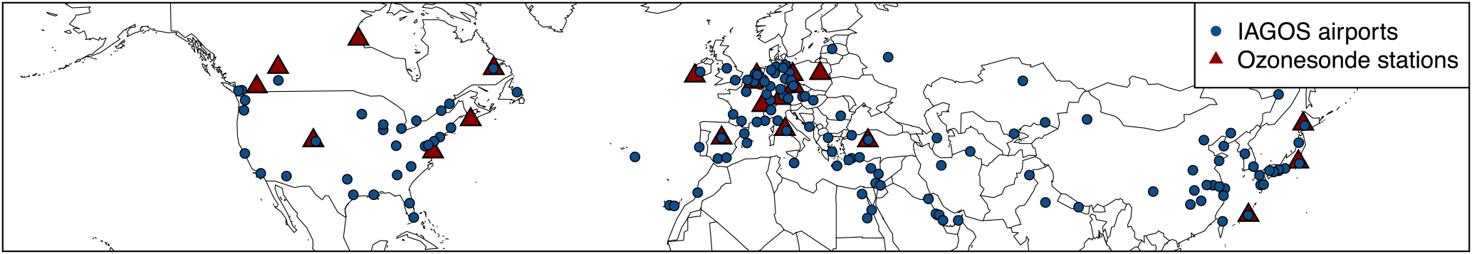
This study focuses on the northern mid-latitudes (25–60∘ N) in order to avoid ill-defined PBL in the tropics due to deep convection and sparse data in boreal and polar regions. In this region, IAGOS profiles are available at 135 airports and ozonesonde profiles at 20 stations, as shown in Fig. 1. The number of profiles available over the period 1994–2016 is 20 762 for the ozonesondes and 72 382 for IAGOS, which represents a total of 93 144 profiles. For both IAGOS and ozonesondes, most profiles are sampled in Europe and North America (especially in the north-eastern United States), with a few in East Asia and the Middle East. It is worth noting at this stage that as O3 and CO mixing ratios can strongly vary from one location to the other, the PBL-referenced profiles that will be obtained from all profiles available at northern mid-latitudes are not expected to be representative of any location in this large latitudinal band. As profiles often show a very complex structure, aggregating such a large number of profiles allows for the smoothing of the vertical distribution and subsequently highlighting specific features. The idea of this study is to focus on the vertical stratification (i.e. the relative changes in mixing ratios with altitude) of O3 and CO rather than their mixing ratios themselves.
All profiles are expressed in metres above ground level (a.g.l.). Note that the altitude available in the IAGOS database corresponds to the barometric altitude above sea level (a.s.l.) estimated from the temperature and pressure measured by the aircraft, assuming standard conditions at the surface (temperature of 288.15 K, pressure of 1013.25 hPa). This leads to an uncertainty on the actual altitude of the aircraft. Under some atmospheric conditions (cyclonic conditions, for instance), the barometric altitude of the aircraft may be below the airport elevation. Without any information on the temperature and pressure at the surface close to the airport, it is not possible to get a more accurate estimation of the altitude. In this study, the altitude a.g.l. is deduced from the barometric altitude a.s.l. available in the IAGOS database by subtracting its first value measured by the aircraft, assuming that this first measurement of the profile is performed close to the surface. The IAGOS measurements are indeed programmed to start when the aircraft wheels leave (or touch) the ground. Some technical issues delaying the beginning of the measurements may occur, but this is expected to concern only a minor proportion of the profiles. Note that the GPS altitude has been available in the IAGOS database only since 2014.
For convenience, all profiles are linearly interpolated at a vertical resolution of 50 m from the surface (thus, this value of 50 m is to be considered as the truncation error in our study). This value was chosen following the sensitivity analysis on the vertical resolution (from 1 to 10 hPa, i.e. about 10 to 100 m) recently performed by Liu and Liang (2010), who concluded that it represents a good compromise between accuracy and uncertainty related to data noise. A sensitivity test with a vertical resolution of 100 m (not shown) confirmed the low sensitivity of the results to this parameter. Additionally, at any given (50 m deep) level, no interpolation is performed when the vertical distance between the two neighbouring points of the raw vertical profile used for the interpolation exceeds 100 m. In this case, the data are considered missing.
As the PBL characteristics exhibit strong diurnal variations, profiles used in this study are separated into different time slots: night (sunset to sunrise), morning (sunrise to solar noon), midday (solar noon to 3 h past solar noon), afternoon (3 h past solar noon to sunset), daytime (sunrise to sunset) and the whole day (denoted “all” in the figures). All time zones and daylight saving hours are properly taken into account.
2.3 Estimation of PBL heights
Three types of PBL can be distinguished: the convective boundary layer (CBL) often occurring during daytime and characterized by strong turbulent mixing under the effect of convective thermals, the stable boundary layer (SBL) occurring mainly during night-time and characterized by the absence of turbulence mixing, and the residual layer (RL) occurring mostly during the night and morning and corresponding to the former CBL, usually delimitated by the SBL top and the capping inversion (Stull, 1988). In our study, for all individual profiles, we first look for any surface-based inversion (SBI) of temperature defined as a monotonic increase in (absolute) temperature from the surface up to a certain altitude (corresponding to the top of the SBI). When no SBI is found, numerous methods have been proposed over the past decades for estimating the PBL height (see Seibert et al., 2000, for a review), including the following: (i) the elevated inversion (EI) method in which the PBL top is located at the bottom of an elevated (absolute) temperature inversion; (ii) methods based on the search for an extremum of vertical gradient in the vertical profile of a relevant thermodynamic parameter (e.g. RH, potential temperature, refractivity); and (iii) methods in which the profile is scanned upward in order to identify at which altitude a certain thermodynamic parameter (e.g. virtual potential temperature, bulk Richardson number) equalizes or exceeds by a certain amount its surface value. Strong systematic differences in PBL height are found among these methods, both in terms of magnitude and seasonal–diurnal variability (e.g. Seidel et al., 2010; Wang and Wang, 2014). The reasons for the discrepancies between the methods are complex (and not clearly understood yet), but may comprise a poor vertical mixing of the PBL, the strong influence of the surface measurement (specifically for the last class of methods), the existence of clouds and/or the uncertainties on the RH measurements under cloudy conditions (Wang and Wang, 2014). As no consensus currently exists, we decided to retain the EI approach in which the PBL top is estimated as the first altitude above which the (absolute) temperature monotonically increases with altitude. The vertical gradient of temperature between the top and the bottom of the EI corresponds to the intensity of the inversion. We require that the difference of temperature between the EI base and the altitude level right above exceeds the value of 0.3 K in order to avoid erroneous identification of the EI base due to uncertainties on the temperature measurements estimated at ±0.25 K in IAGOS (Berkes et al., 2017). All profiles with no or too-weak (below 0.3 K) temperature inversion are discarded. Two examples of profiles are presented in Fig. 2. Note that as it relies only on temperature and not on RH measurements (that are not always fully available over the profiles since all RH data flagged as “doubtful” in IAGOS are rejected), the EI method allows us to maximize the number of profiles taken into account for deriving the climatological vertical distribution of O3 and CO.
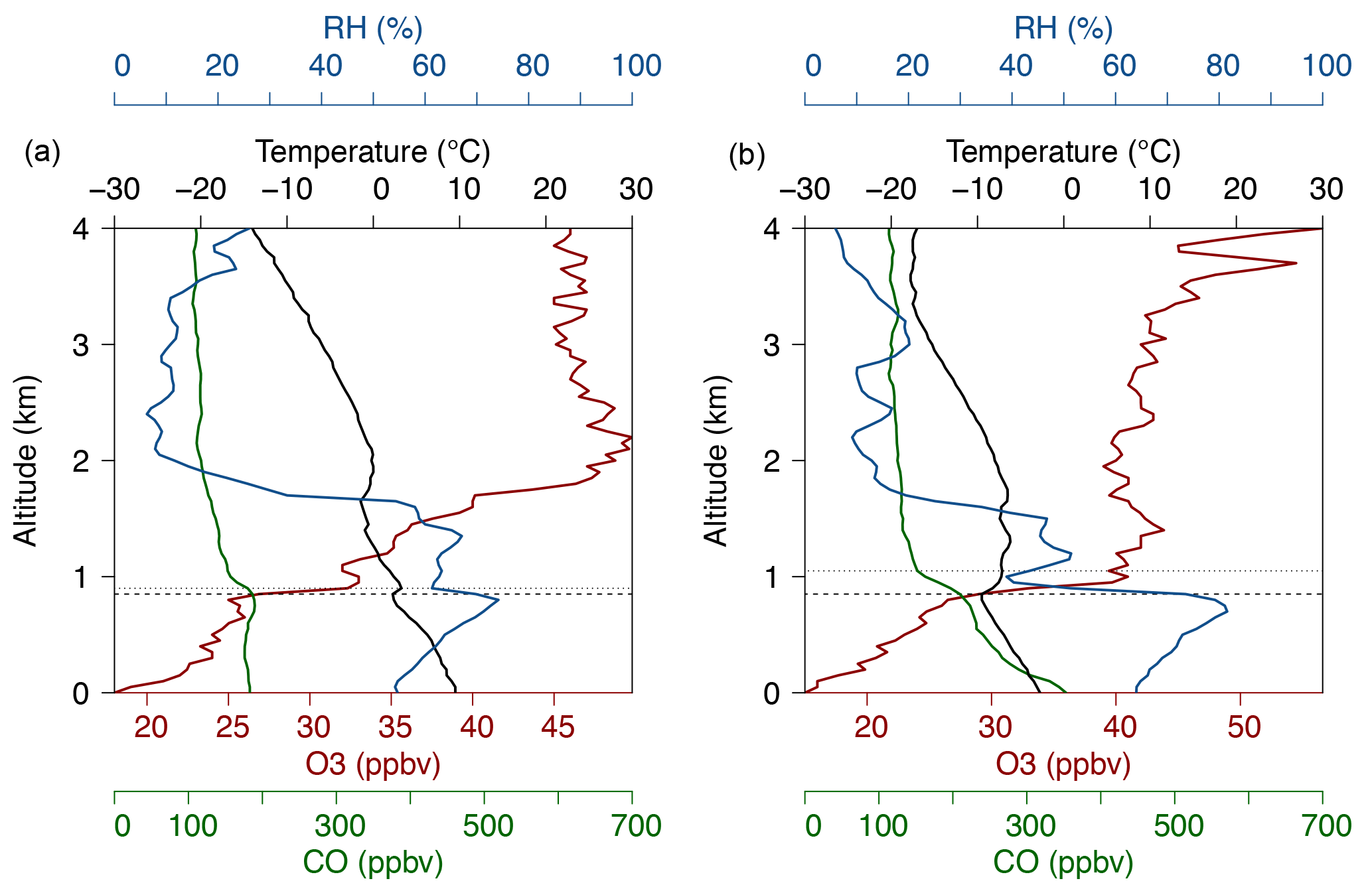
Figure 2Vertical profiles measured by IAGOS on 2004/11/28 (flight no. 10275975, a) and 2004/12/22 (flight no. 10451135, b). The curves display the profiles of O3 (red line) and CO (green line) mixing ratios, RH (blue line) and temperature (black line). The plot also shows the base (dashed black line) and top (dotted black line) of the elevated temperature inversion.
Although the EI represents a real geophysical interface between two layers, it is important to note at this stage that this height does not necessarily always correspond to the height of the mixing layer as it may, for instance, correspond to the capping inversion aloft of the residual layer (rather than e.g. the top of an instable nocturnal boundary layer or a growing CBL in the morning). For convenience, we will hereafter refer to the PBL height but the reader should keep in mind that this term may sometimes be ambiguous.
Following previous studies (e.g. Seidel et al., 2010; Wang and Wang, 2014), a maximum PBL height of 4000 m a.g.l. is fixed. In order to further avoid erroneous PBL height estimations due to too-large data gaps in the profile, we require at least 75 % of available data between 0 and 4000 m a.g.l. In addition, for all PBL calculations, we require a maximum of 200 m (i.e. four 50 m deep levels) with missing data between the surface and the estimated PBL height. Among the 93 144 profiles available, SBI and EIs are found in 16 and 63 % of the profiles, respectively. The remaining profiles (21 %) either do not fulfil the previous criteria (due to data gaps) and/or show no significant temperature inversion in the first 4000 m a.g.l. and are thus discarded.
In this section, we analyse the climatology of the PBL heights obtained from the IAGOS and ozonesonde profiles by distinguishing the case of SBIs (Sect. 3.1) and EIs (Sect. 3.2).
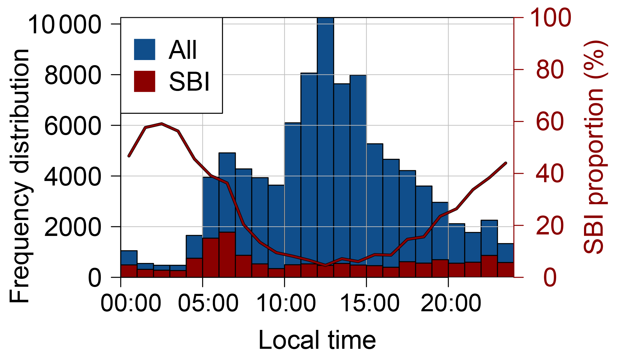
Figure 3Frequency distribution of the measurement time of all vertical profiles (blue bars; left axis) and the profiles on which an SBI is detected (red bars superposed over blue ones; left axis). The corresponding proportion of SBI is also plotted (red line; right axis).
3.1 Surface-based inversions (SBIs)
SBIs are important features for air pollution as they inhibit the vertical mixing of pollutants released at the surface. Concerning ozone, they can induce a strong depletion either by dry deposition or titration by the nitrogen oxide (NO) accumulated at the surface (Colbeck and Harrison, 1985). The distribution of the local time (LT) at which (IAGOS and ozonesondes) profiles are measured is shown in Fig. 3 with the proportion of SBI occurrences. Most of the available profiles are measured between 05:00 and 19:00 LT. Results highlight a strong diurnal variability in these SBIs and their characteristics. As expected, they are the most frequent during the night when their proportion continuously increases up to a maximum of 60 % at 03:00 LT (red curve in Fig. 3). Thus, although SBIs are more frequent during the night, many night-time profiles still show unstable conditions. At the locations close to large agglomerations (e.g. airports), the absence of SBIs during the night may be partly due to the urban heat island phenomenon that can turn a stable PBL into a near-neutral PBL (Dupont et al., 1999). The proportion of SBIs then progressively decreases to a broad minimum of 5–10 % between 10:00 and 17:00 LT. Very similar diurnal variations in the proportion of SBIs are observed during all four seasons (not shown).
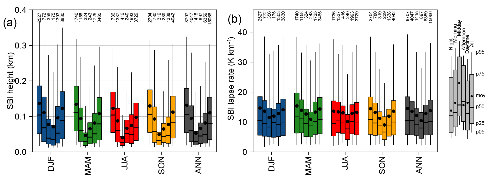
Figure 4SBI height (a) and temperature lapse rate between the surface and the top of the SBI (b). Results are shown for each season (one colour per season) and for the different time slots (adjacent bars from left to right: night, morning, midday, afternoon, daytime, entire day; the legend is indicated in grey on the right side). The number of profiles for each bar is indicated on the graph.
Both the height and the temperature lapse rate (vertical gradient of temperature between the surface and the SBI top) of these SBIs are shown with their diurnal and seasonal variations in Fig. 4 (considering both IAGOS and ozonesonde profiles). SBIs occur all year with almost no seasonal variations in their frequency. This type of inversion leads to very shallow stable layers with a mean depth of 110 m. A moderate seasonal variability of 23 % is highlighted (as calculated as the difference between the maximum and the minimum SBI height normalized by the annual SBI height), with mean SBI heights ranging from 97 m in summer to 123 m in winter. However, the diurnal variability of the SBI height is strong (71 %), with the largest SBIs being observed during night-time (131 m on annual average) and the smallest during midday (53 m on annual average). The 95th percentile reaches about 300 m. This is substantially lower than the SBIs reported by Seidel et al. (2010), whose median heights ranged around 200–500 m. Differences may be (at least partly) due to the fact that our results are based on profiles measured at northern mid-latitude stations (most of them being located in the latitudinal band 35–55∘ N) essentially during daytime, while the dataset analysed by Seidel et al. (2010) extends to stations located further north up to polar regions and includes a predominant proportion of night-time–morning radiosonde profiles. On average, the temperature lapse rate is about 13 K km−1, with moderate seasonal differences (12 %). Some diurnal variations are also observed during most seasons, with usually decreasing temperature lapse rates from night-time to the afternoon.
3.2 Elevated temperature inversions (EIs)
We investigated some characteristics of the EIs, namely the temperature difference, width and temperature vertical gradient (see Fig. S1 in the Supplement). The difference in temperature between the base and the top of the EIs is 1.5 K on annual average, with strong seasonal variations from 1.1 K in summer to 2.1 K in winter. The 95th percentile also exhibits high seasonality with values ranging from 3.3 K in summer to 7.2 K in winter. The mean width of these EIs increases from 76 m in summer to 103 m in winter, in reasonable agreement with EI thicknesses estimated by other authors (e.g. Cohn and Angevine, 2000). This leads to mean temperature vertical gradients of 1.4 and 1.9 K hm−1 (where hm stands for hectometre, i.e. 100 m) during these two seasons, respectively. Interestingly, none of these characteristics exhibits diurnal variation (whatever the statistical metric).
The seasonal and diurnal variations in the PBL height estimated with the EI method are shown in Fig. 5 for all seasons and time slots. Averaged over all profiles, the mean PBL height is 1253 m, with values ranging from 1132 m during the night to 1483 m in the afternoon. This corresponds to diurnal variability of 28 %, the diurnal variability here being calculated as the maximum minus minimum PBL height normalized by the mean PBL height based on the values available during the different time slots shown in Fig. 5 (for this example (1483−1132) × 100/1253 = 28 %). Such high night-time values and moderate diurnal variability indicate that the EI height often corresponds to the top of the nocturnal RL (as previously mentioned in Sect. 2.3). As expected, the diurnal variability is much lower in winter (17 %) than in the other seasons (30–38 %). The highest PBL heights are observed during summertime afternoon with 1707 m on average. Similarly, the seasonal variability strongly varies with the time of day, with values of 22, 23, 32 and 35 % during the night, morning, midday and afternoon, respectively.
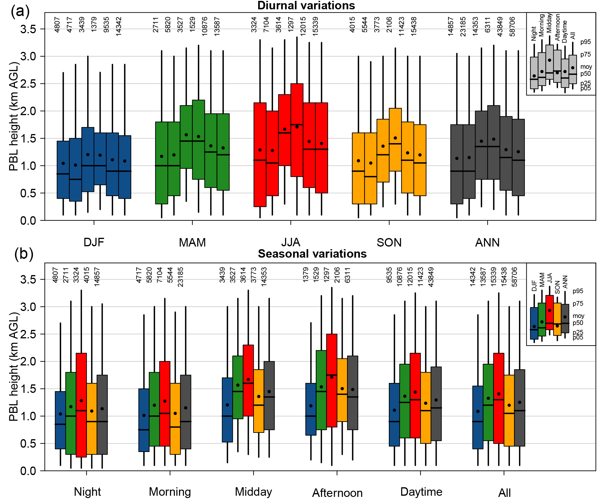
Figure 5Diurnal (a) and seasonal (b) variations in the averaged PBL heights. For all combinations of season and time of day, the number of available profiles is indicated above the box plot.
In this section, we investigate the climatological vertical stratification of two thermodynamic parameters (RH, θ) and two trace gases (O3, CO) within the PBL (estimated with the EI method) and at the PBL–FT interface. Due to the variations in PBL height from one profile to the other, calculating a climatological profile by simply averaging all individual profiles inevitably smoothes all the vertical features that may exist for some compounds or meteorological parameters, especially at the PBL–FT interface. In order to highlight how the PBL height influences these vertical distributions, all individual vertical profiles are thus first expressed in a vertical coordinate system based on the PBL height and then averaged. In practice, all individual profiles are expressed as a function of z∕h with z the altitude and h the PBL height estimate, with z∕h ranging from 0 to 2 (in bins of 0.05). For instance, if the PBL height on a specific profile is 1000 m, the resampled profile will extend from 0 to 2000 m (with bins of 50 m). Hereafter, this type of vertical profile is denominated as a PBL-referenced vertical profile. Then, all these PBL-referenced profiles are averaged to derive a climatological vertical distribution apart from the PBL–FT interface. Hereafter, the PBL–FT interface will be designated by the 1 altitude level (which means that the entrainment zone is here included in the FT).
In order to illustrate the usefulness of this approach, we consider an artificial dataset of vertical profiles characterized by the presence of a discontinuity at the PBL top (h), here arbitrarily chosen as a step function with different but constant mixing ratios below (c1) and above (c2) this interface. A dataset of 50 profiles is generated by choosing random integers between 10 and 30 ppbv for c1, between 20 and 40 ppbv for c2, and between 100 and 1500 m for h. All these profiles are superposed in grey in Fig. 6a, including one individual example in black (for which c1=15 ppbv, c2=38 ppbv and h= 1200 m). In such a dataset, the mean vertical distribution (red curve in panel a) is characterized by an overall increase in the mixing ratios with altitude (up to 1500 m, the upper bound fixed in this example). The discontinuity introduced in all individual profiles is entirely smoothed in this mean profile, as shown by the gradient profile (red curve in panel b). If all these profiles are first normalized by the PBL height (grey curves in panel c) and then averaged (blue curve), the discontinuity of the mixing ratios is preserved, as clearly shown by the PBL-referenced gradient profile (panel d). For comparison with the traditional profiles, both the PBL-referenced profile and gradient profile were dilated using the mean PBL of this dataset (about 900 m in this example) and added to the first series of plots (blue curves in top panels). Considering PBL-reference profiles thus allows us to investigate the features (or in other words, any kind of discontinuity) that may exist at the PBL top.
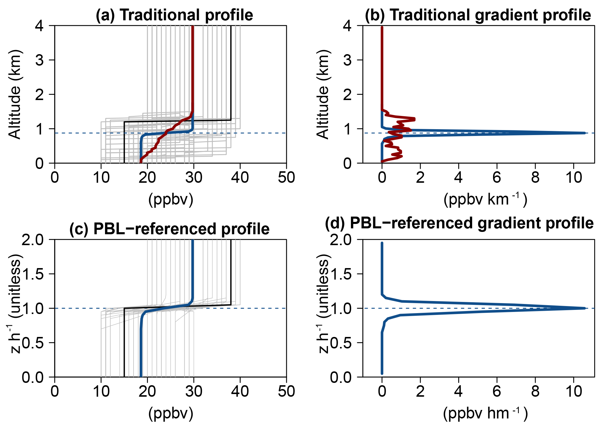
Figure 6Artificial vertical profiles (a, c) and gradient profiles (b, d) expressed as a function of z (a, b) and z∕h (c, d). The figure shows all individual profiles (grey lines), one example of an individual profile (black line), the z-referenced mean profile (red line) and the PBL-referenced profile (blue line), and the mean PBL height of this artificial dataset (blue dotted line; see text for details).
Only complete profiles (i.e. with available data at all z∕h from 0 to 2) are averaged together. This is an important restriction which limits the number of profiles but ensures the most reliable vertical distribution when averaged. Note that we tested to fill the small data gaps (width up to 100 m included) by interpolation using natural cubic splines. As this only increases the number of profiles by about 10 % (which means that the data gaps are usually larger than 100 m) and does not change the climatological results, we decided to not use any interpolation to fill the data gaps in the profiles. The number of complete profiles is finally 43 244 for the potential temperature, 17 649 for RH, 30 960 for O3 and 8295 for CO.
In the following sections, the PBL-references profiles are presented for θ (Sect. 4.1), RH (Sect. 4.2), CO (Sect. 4.3) and O3 (Sect. 4.4) based on the profiles on which an EI is identified. Mean profiles will be shown for the different seasons and time slots. However, it is worth noting that the climatological profiles at the different time slots are not directly comparable with each other since they are calculated based on profiles sampled at different periods and locations. The profiles of (local) vertical gradients will also be analysed. Note that for all variables discussed in Sect. 4 (θ, RH or mixing ratios), these profiles of vertical gradients will be expressed in the common unit of the variable (∘C, % or ppbv) per hectometre (hm−1) as it keeps most numbers in the range of 0.1–10.
4.1 Potential temperature
The PBL-referenced profiles of potential temperature in the absence of SBI (and in the presence of an EI) are shown in Fig. 7. On average, the potential temperature is found to be slightly superadiabatic in the surface layer (i.e. θ decreases with altitude) during both morning (−0.08 ∘C hm−1) and midday (−0.13 ∘C hm−1). The width of this superadiabatic layer never exceeds 5–10 % of the PBL height.
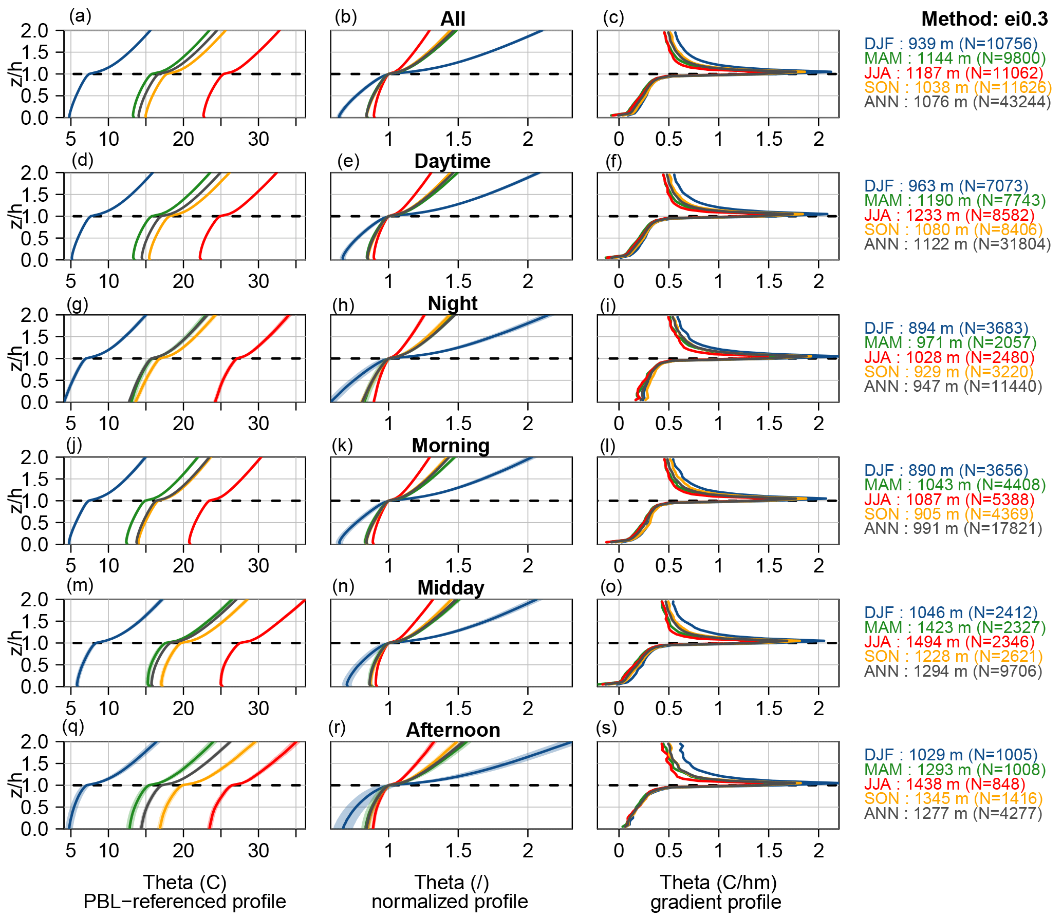
Figure 7Vertical profiles of potential temperature (in ∘C; a, d, g, j, m, q); the same profiles normalized by the potential temperature at 1 (b, e, h, k, n, r) and vertical gradient profiles (in ∘C hm−1; c, f, i, l, o, s). Plots are shown for different time slots (from top to bottom: all day, daytime, night-time, morning, midday, afternoon). The shaded area represents the uncertainties (at a 95 % confidence level) on the mean. For each season and time of day, we indicate the number (N) of profiles used for calculating the PBL-referenced profile (i.e. profiles without any missing data) and the mean PBL height calculated based on this subset of profiles.
Above that surface layer, the potential temperature increases with altitude. While neutral adiabatic profiles (i.e. no variations in θ with altitude) were expected within the convective PBL, at least during daytime (Stull, 1988), all climatological profiles appear subadiabatic (positive vertical gradient of θ). This subadiabatism varies with the season with strongest values in spring–winter (0.51 ∘C hm−1 on average over the PBL) and lowest values in summer (0.25 ∘C hm−1). As expected, a very sharp increase in the potential temperature is highlighted at the top of the PBL where vertical gradients reach +1.3 ∘C hm−1 on average. This maximum gradient is found to be much higher in winter (+1.6 ∘C hm−1) than in summer (+1.1 ∘C hm−1), as previously analysed (see Sect. 3.2). These seasonal variations are the strongest during the afternoon (+1.8 and +1.0 ∘C hm−1 in winter and summer, respectively). Above, in the lower FT, the increase in temperature with altitude is reduced but remains higher than in the PBL.
As mentioned in Sect. 2.1, several important differences of sampling exist between these two datasets, including the fact that (i) IAGOS aircraft fly at a 30 % higher descent–ascent rate and cover a horizontal distance 10 times larger in the lower troposphere, and (ii) IAGOS measurements are performed in the vicinity of international airports and large agglomerations, while ozonesonde stations are usually located in remote, rural or low-density urban areas (leading to a population density around IAGOS airports of about 2000 inhabitants km−2 on average within ±0.1∘ in longitude and latitude against about 1150 inhabitants km−2 for ozonesonde stations; see Sect. S1 in the Supplement for details). This raises the question of whether or not these sampling differences impact the PBL-referenced vertical distribution. Answering this question would require collocated (in time and space) IAGOS and ozonesonde profiles, but far too few profiles fulfil these conditions. However, in order to give some insights about this question, we calculated the climatological profiles from both datasets taken separately (Fig. 8). Only daytime profiles are shown as ozonesondes and are much sparser during the night. Again, these PBL-referenced profiles obtained with IAGOS and ozonesondes are not expected to be the same since they are sampled in different locations and times and thus correspond to different PBL heights; considering the profiles used in Fig. 8, the mean PBL height is 10–20 % higher in ozonesondes than in IAGOS profiles depending on the season.
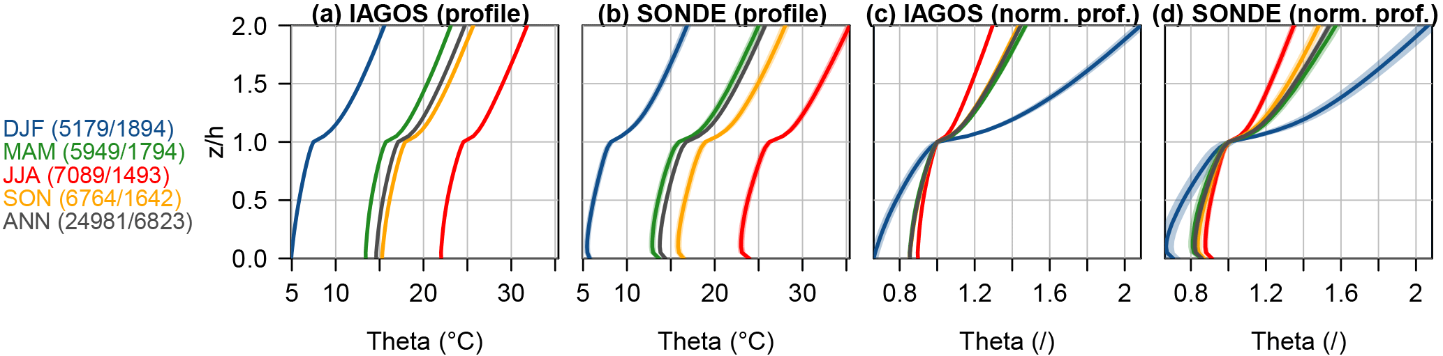
Figure 8IAGOS and ozonesonde PBL-referenced (a, b) and normalized profiles (c, d) of daytime potential temperature. The number of profiles accounted for is indicated for each season (in brackets: IAGOS ∕ SONDE).
Results obtained using both datasets are in reasonable agreement. The main difference is found near the surface where only ozonesondes highlight a small superadiabatism. This may be partly due to the fact that in contrast to ozonesondes, IAGOS measurements do not start at the surface but at a minimum height of a few metres a.g.l. (since instruments are located in the lower part of the fuselage). However, as individual IAGOS profiles sometimes do show a superadiabatism at the surface, the main reason is more likely related to the inherent uncertainties of the IAGOS barometric altitude, which is deduced from the pressure assuming standard atmospheric conditions at the surface (as explained in Sect. 2.2). This may partly smooth the superadiabatism at the surface (as the mean potential temperature in the first 0–50 m altitude level would include some points actually outside the 0–50 m layer and/or ignore some other points actually belonging to this layer). At the annual scale, considering all time slots and z∕h levels, the mean bias (MB), root mean square error (RMSE) and correlation (R) between the PBL-referenced profiles of both datasets are 2 ∘C, 3 ∘C and 0.97, respectively (with ozonesondes here taken as the reference).
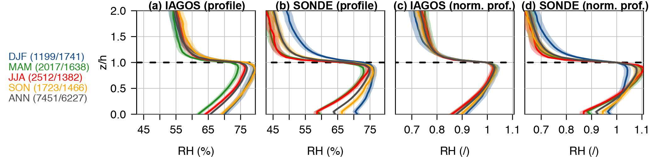
Figure 10IAGOS and ozonesonde PBL-referenced (a, b) and normalized profiles (c, d) of daytime RH. The number of profiles accounted for is indicated for each season (in brackets: IAGOS ∕ SONDE).
4.2 Relative humidity
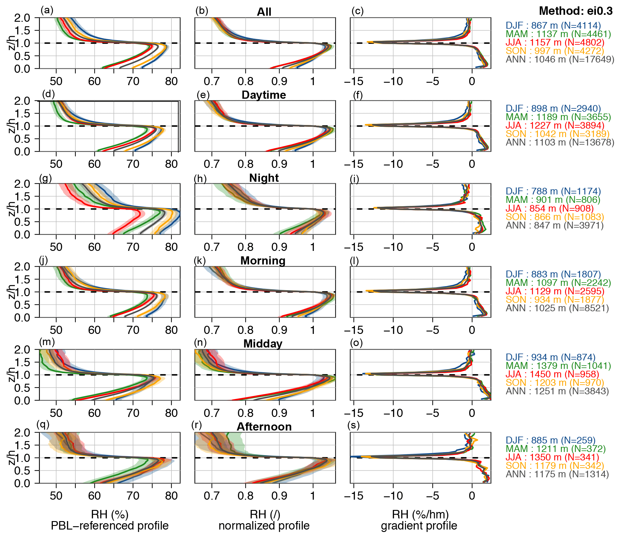
The PBL-referenced profiles of RH are shown in Fig. 9. At the surface, the mean RH ranges between 55 and 80 % with a well-known seasonal and diurnal pattern characterized by highest values during the wintertime nights and lowest values during the springtime–summertime afternoons. As one moves higher in altitude, RH increases quite regularly up to a maximum located around 0.8, which is thus just below the top of the PBL. At this level, RH values range between 70 and 85 %. The seasonal differences persist but the diurnal ones are greatly reduced (the absolute difference between the night-time maximum and the afternoon minimum remains below 10 %). A sharp decrease in RH is observed at the PBL–FT interface. The vertical gradient reaches its minimum right above the PBL top (at 1.05) with −12 % hm−1 on average. The diurnal and seasonal variability of these strongest RH gradients remains low (between −11 and −15 % hm−1). In the lower FT, RH decreases with altitude, usually with stronger (negative) gradients in winter than in summer.
The PBL-referenced vertical profiles of RH obtained with IAGOS and ozonesondes taken separately are shown in Fig. 10. Although the shape of the profiles remains in reasonable agreement, some differences are highlighted. In particular, ozonesondes show a stronger RH vertical gradient within the PBL and a sharper decrease in the lowermost FT with much lower RH in the FT. This sharper decrease above the PBL top might be due to the fact that, as briefly mentioned in Sect. 2.1.2, RH measurements with radiosondes are generally affected by a radiation dry bias due to the heating of the sensors by solar radiation, which can lead to a negative bias on the RH measurements of the order of 5–10 % in the lower troposphere (e.g. Vömel et al., 2007; Bian et al., 2011; Wang et al., 2013). In our case, this bias could be further enhanced in the lower FT due to solar reflection by clouds at the top of the PBL. This is also supported by the fact that the differences between IAGOS and sondes are largely reduced when considering only night-time profiles, i.e. when radiosonde measurements are not affected by heating effects due to solar radiation (not shown). These sources of bias are also expected to vary from one season to the other following the seasonality of solar radiation that is strongest in spring–summer and lowest in winter–fall. This may (at least partly) explain the distortion of the seasonal variations of RH in ozonesondes compared to IAGOS in the lower free troposphere. At the annual scale, taking into account all time slots and z∕h levels and considering ozonesondes as the reference, the comparison between IAGOS and ozonesonde datasets gives MB, RMSE and R of +0 %, 9 % and 0.67, respectively.
4.3 Carbon monoxide
The PBL-referenced profiles of CO are shown in Fig. 11. The uncertainties of these mean profiles are substantially higher than for the previous meteorological parameters, notably due to a much lower number of measurements (as CO is only measured by IAGOS aircraft and starting from 2002). Considering all profiles, the mean CO mixing ratios at the surface increase from about 240 ppbv in summer to 340 ppbv in winter. The CO mixing ratios decrease with altitude at a varying rate depending on the altitude. The normalized profiles (Fig. 11b, e, h, k, n, r) show that the difference in CO between the surface and the PBL top reaches a factor of 1.3 on average. The first important result shown by these PBL-referenced profiles is therefore the substantial vertical stratification of CO mixing ratios within the PBL.
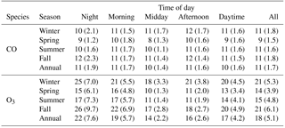
In order to investigate that stratification on a quantitative basis, we introduce a first factor of vertical stratification (γ) here defined as the standard deviation of the mixing ratio profile between the surface and the PBL top (i.e. over the 21 z∕h levels comprised between 0 to 1) normalized by the mean. We also define a second factor of vertical stratification (δ) calculated by normalizing γ by the PBL height. The calculations are first done on each individual profile and then averaged over all profiles. The γ and δ factors will be expressed in % and % hm−1, respectively. Results are reported in Table 2 for the different seasons and time slots. On average, the γ factor of CO vertical stratification is 11 % and varies little with the season and time of day (from 8 to 12 %), the strongest values usually being found in winter–fall. The δ factor exhibits relatively stronger variations, with values ranging from ∼ 1 % hm−1 during summer midday to more than ∼ 2 % hm−1 during winter–fall night.
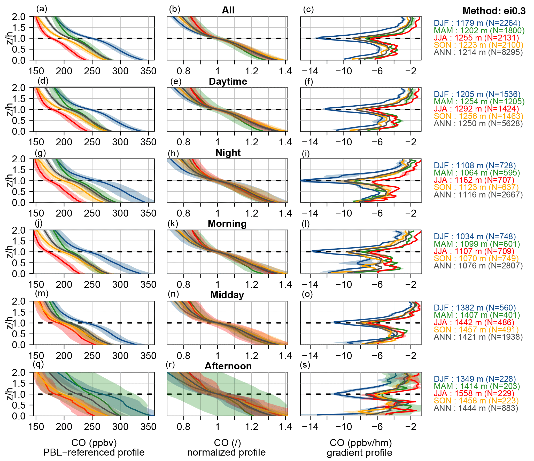
The strongest vertical gradients are observed at the PBL top and close to the surface. At the PBL top, the strong vertical gradients involve the presence of a clear inflexion point in the mean CO profile (as shown by gradient profiles in the right panels of Fig. 11). With a traditional vertical coordinate system (i.e. z rather than z∕h), this feature would have been smoothed (see Fig. 6). The presence of this inflexion point on an independent variable (i.e. a variable not used in the estimation of the PBL height) gives confidence in our ability to capture reasonably well a real geophysical interface with the EI approach. It illustrates the fact that as expected, EIs act as an effective although porous geophysical barrier that limits the vertical exchanges between the PBL and FT, leading to a distinct chemical composition on each side. The sharp gradients at the PBL–FT interface are strongest in winter and lowest in summer. Such seasonal variations are consistent with the fact that EIs are deeper and characterized by a stronger temperature gradient in winter than in summer (as previously shown in Sect. 3.2), which greatly inhibits the ventilation of the polluted PBL and the exchanges with the cleaner FT. The strong gradients at the surface ensue from the presence of CO emissions and are usually maximum during night-time and morning. Substantially lower vertical gradients are found in the FT.
Table 2Factors of vertical stratification γ (in %) and δ (in % hm−1; in brackets) of O3 and CO in the PLB for the different seasons and time slots (see text for details on their calculation).
4.4 Ozone
4.4.1 PBL-referenced vertical distribution of O3
Figure 12 presents the mean PBL-referenced profiles of O3 in which all profiles sampled at northern mid-latitude stations are aggregated. It is worth noting that both the surface mixing ratio and vertical distribution of O3 are highly variable in both time and space and can greatly change depending on the meteorological conditions and the availability of O3 precursors. At the scale of individual profiles, the O3 vertical distribution is often very complex with persistent layering. In our study, taking into account a very large number of profiles allows us to obtain well-smoothed PBL-referenced profiles (Fig. 12) with low layering and therefore to highlight some general background characteristics of the O3 vertical stratification in the lower troposphere.
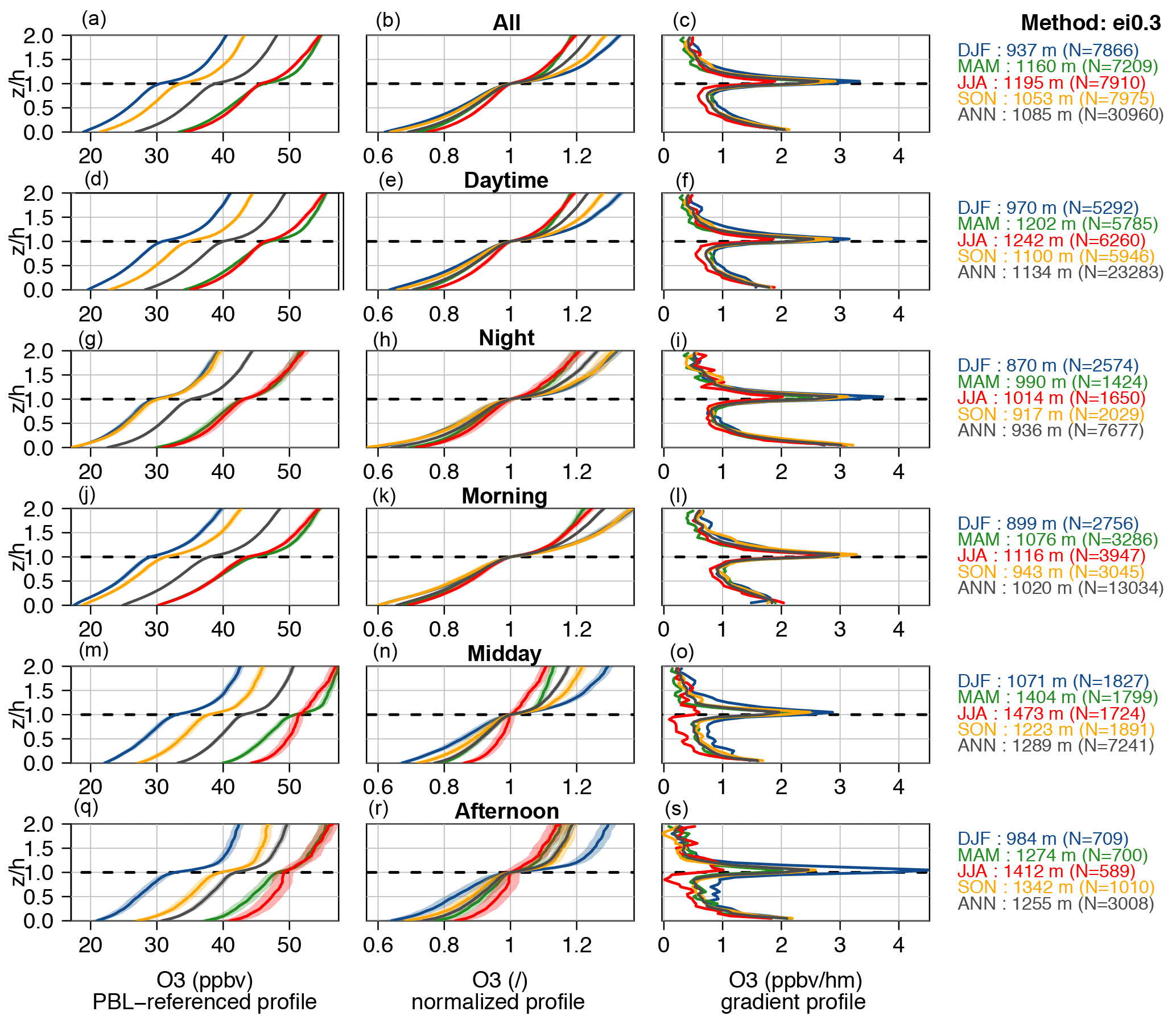
On average over all profiles, surface O3 mixing ratios range between 20 ppbv in winter–fall and 30–35 ppbv in spring–summer. Above the surface, the O3 mixing ratios increase with altitude through the whole PBL and the lower FT with vertical gradients displaying strong variations depending on the season and altitude (relatively to the PBL top). As for CO, the strongest gradients are observed both close to the surface and at the PBL–FT interface. Close to the surface, they are likely explained by the strong intensity of the main O3 sinks, namely dry deposition and titration by the NO emitted by anthropogenic emission sources. The combination of these two sinks leads to sharper vertical gradients for O3 than for CO (relatively to mixing ratios). The maximum vertical gradient at the surface is observed during the night (around 3 ppbv hm−1). The rate of O3 increase with altitude slightly decreases with altitude in the PBL. A clear inflexion point is highlighted at the interface between the PBL and FT ( 1). Compared to CO, this inflexion point in O3 profiles is usually much sharper. Such a difference suggests that, (i) while the smooth CO inflexion point mostly results from the limited vertical exchanges between the PBL and FT in the presence of the EI, (ii) the stronger O3 inflexion point is not only due to this dynamical effect but also to a difference in chemical regime apart from the PBL–FT interface. In other words, results suggest that the CO inflexion point is mostly driven by dynamics (since the CO chemical reactivity is low), while the O3 inflexion point is driven by both dynamics and chemistry. The vertical gradient at the PBL top is found to strongly vary with the season with the sharpest increase in winter and a much smoother increase in summer. While this strong gradient persists all day in winter, it is found to be lower in midday–afternoon during summertime. This is likely due to the combined effect of the efficient photochemical production of O3 in the PBL and the entrainment of O3-rich air masses from the FT. The entrainment can indeed play a strong role in the O3 budget within the PBL, comparable to advection or deposition, as recently highlighted by Trousdell et al. (2016). Higher in altitude in the lower FT, the increase in O3 mixing ratio with altitude is found to be substantially smaller than in the PBL.
Based on 214 aircraft vertical profiles obtained during the DISCOVER-AQ (Deriving Information on Surface conditions from Column and Vertically Resolved Observations Relevant to Air Quality) and the FRAPPÉ (Front Range Air Pollution and Photochemistry Éxperiment) campaigns in Colorado during summer 2014, Kaser et al. (2017) recently investigated the O3 vertical gradient between the PBL and the lower FT in order to estimate this O3 entrainment in the PBL and to evaluate its representation in the WRF-Chem model. The difference in O3 mixing ratio between the PBL and the (arbitrary chosen) 300 m wide layer above the PBL top was found to vary from +9 ppbv in the morning to −11 ppbv in the afternoon (the negative value meaning that higher O3 mixing ratios are measured in the PBL). This differs from our climatological results in which the summertime O3 vertical gradients at the PBL–FT interface also decrease from the morning (2.5 ppbv hm−1) to the afternoon (0.9 ppbv hm−1) but remain positive (i.e. O3 mixing ratios in the FT remain higher than in the PBL). However, if we consider only the ozonesonde profiles at Boulder, Colorado (i.e. in the same region where the DISCOVER-AQ campaign took place), our results show a summertime vertical gradient of O3 at the PBL–FT interface close to zero during the late morning and negative at midday (see Fig. S1 in the Supplement), thus in good agreement with Kaser et al. (2017). This suggests that our climatology may not be representative of the most polluted regions during O3 pollution episodes. Our study also agrees with Kaser et al. (2017) on the fact that, even at daytime during summer (when the vertical turbulent mixing is expected to be the strongest), a strong vertical stratification of O3 mixing ratios persists in the lower part of the PBL (the first few hundred metres).
As mentioned at the beginning of this section, comparing the climatological profiles at the different time slots is tricky since they are partly based on profiles sampled at different locations. However, in terms of diurnal variations in O3, the 18 years of IAGOS profiles available at the Frankfurt airport have already been used to demonstrate the clear decrease in diurnal variability with altitude (Petetin et al., 2016).
In terms of vertical stratification within the PBL, the γ and δ factors for O3 are given in Table 2. Considering all profiles, the mean vertical stratification of O3 in the PBL is 18 % (or 5 % hm−1). It ranges from ∼ 10 % (∼ 1 % hm−1) in spring–summer midday–afternoon to ∼ 25 % (7–10 % hm−1) in winter–fall night. This is consistent with a stronger vertical mixing within the PBL associated with higher thermal instability in the PBL under sunny conditions. In order to investigate the influence of meteorological conditions, both stratification factors are calculated for different ranges of surface potential temperature (from −10 to +35 ∘C, with bins of 5 ∘C) considering only daytime profiles (Fig. 13a, b). For comparison, results are also shown for CO (c, d). Note that whatever the season, computing the weighted average of the curve shown in Fig. 13 with weights taken as the number of profiles available at each potential temperature interval allows us to retrieve the mean (daytime) γ factors given in Table 2.
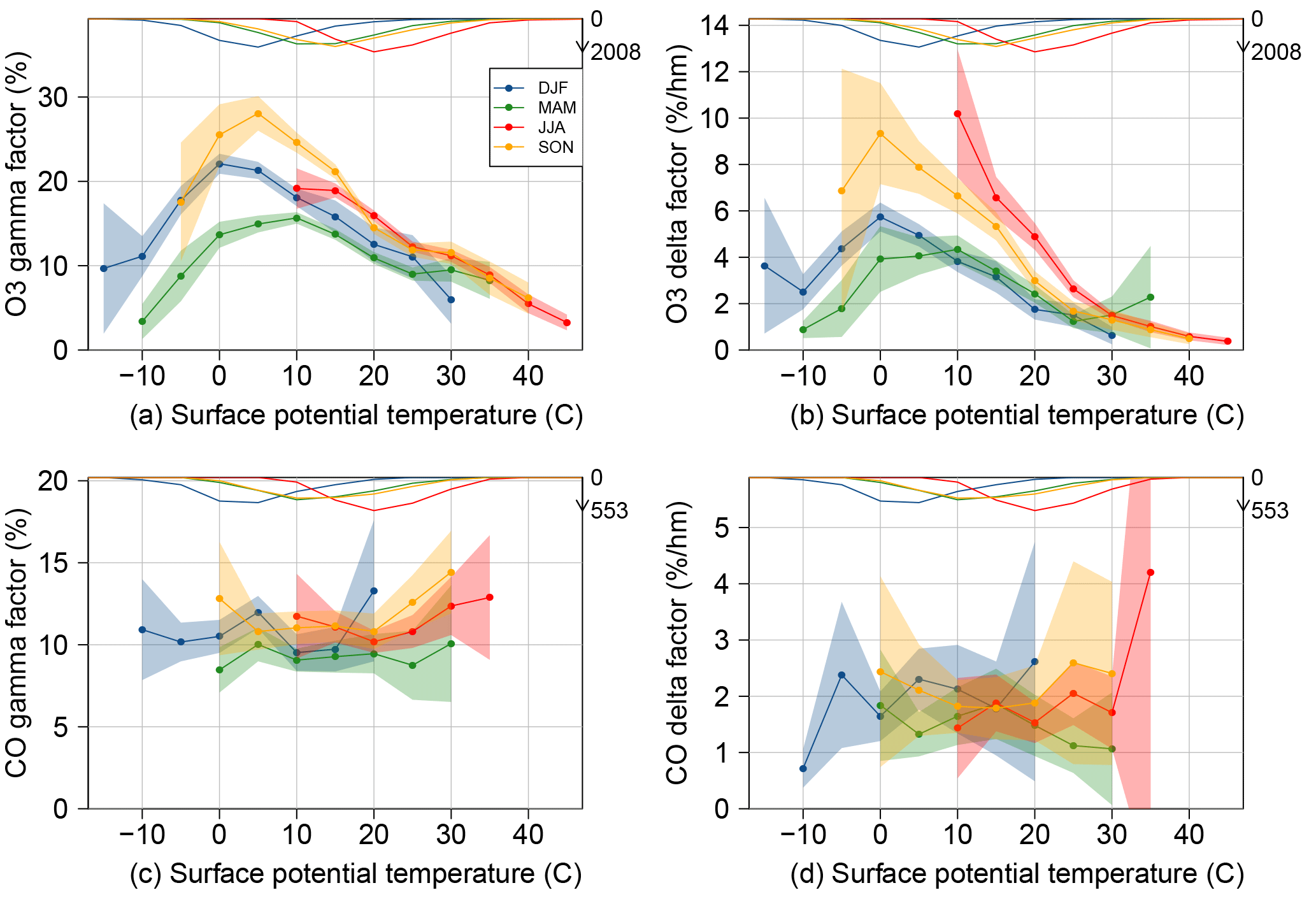
Figure 13Daytime factors of vertical stratification as a function of surface potential temperature. Results are shown for O3 (a, b) and CO (c, d) and for both γ (in %; a, c) and δ (in % hm−1; b, d). The shaded area represents the uncertainties (at a 95 % confidence level) on the mean. The curves at the top of the graph show the number of profiles taken into account (the highest number of profiles is indicated by the arrow).
In contrast to CO vertical stratification factors that do not show clear variations with the surface potential temperature, O3 results highlight an interesting bell shape. The weakest O3 vertical stratification is observed not only at high potential temperatures (above 30 ∘C, when turbulence is expected to be strong due to the heating of the surface), but also at low (typically negative) potential temperatures, while the strongest stratification is observed at intermediate potential temperatures. This behaviour is observed during all seasons (except summer when temperatures remain high enough). During wintertime, a relatively well-mixed O3 profile with moderate mixing ratios is, for instance, frequently observed at stations in northern North America (e.g. Goose Bay, Yarmouth, Churchill). Note that this decrease in the vertical stratification is not due to much lower O3 mixing ratios at the surface (the denominator in the γ and δ formulas) since the latter also follows an (inversed) bell shape with a decrease from 23 to 17 ppbv between −10 and 0 ∘C and an increase up to 48 ppbv at 30 ∘C (see the density scatter plot of O3 mixing ratios versus surface potential temperature in Fig. S2 in the Supplement). Similarly, low standard deviations in O3 profiles within the PBL (the numerator in the γ and δ formulas) are usually found when potential temperatures are negative. The weaker vertical stratification at lower surface potential temperatures illustrates the fact that although this last parameter alone could somehow be a relevant proxy for the static instability within the PBL, the vertical homogeneity of the O3 pollution in this layer is also driven by other mechanisms (e.g. wind, clouds, snow), especially under cold conditions. Concerning the influence of snow, although still very uncertain, much lower O3 deposition rates have been reported in the literature over snow compared to vegetation due to the low reactivity of O3 in pure water (e.g. Stocker et al., 1995; Wesely et al., 1981; Helmig et al., 2007). This could at least partly explain the weaker O3 vertical stratification under low negative surface potential temperatures (while such bell shapes are not observed with CO for which no deposition sink exists), although dedicated studies are obviously required for investigating in more detail the reasons for such a behaviour.
4.4.2 Comparison between IAGOS and ozonesonde profiles
As for the previous meteorological parameters and chemical species, we now investigate how the PBL-referenced profiles obtained from IAGOS and ozonesondes are comparable. The climatological profiles from both datasets taken separately are compared in Fig. 14, considering only daytime profiles. As expected, some quantitative differences in O3 mixing ratios are found between the datasets likely due to their different spatio-temporal distribution at the northern mid-latitudes (IAGOS showing lower mixing ratios). However, the normalized profiles highlight a consistent vertical structure of O3 between IAGOS and ozonesondes, whatever the season. One difference is the slightly less pronounced decrease in O3 right above the EI base in ozonesonde profiles. This could be due to the longer sensor response time of ozonesondes (20–30 s against 4 s for IAGOS) and the subsequent coarser vertical resolution of the sampling that smoothes the sharp vertical gradients in the capping inversion layer more.
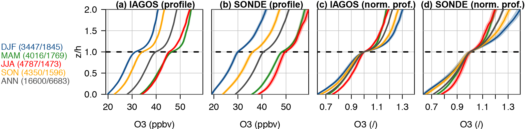
Figure 14IAGOS and ozonesonde PBL-referenced (a, b) and normalized profiles (c, d) of O3 mixing ratios. The number of profiles accounted for is indicated for each season (in brackets: IAGOS ∕ SONDE).
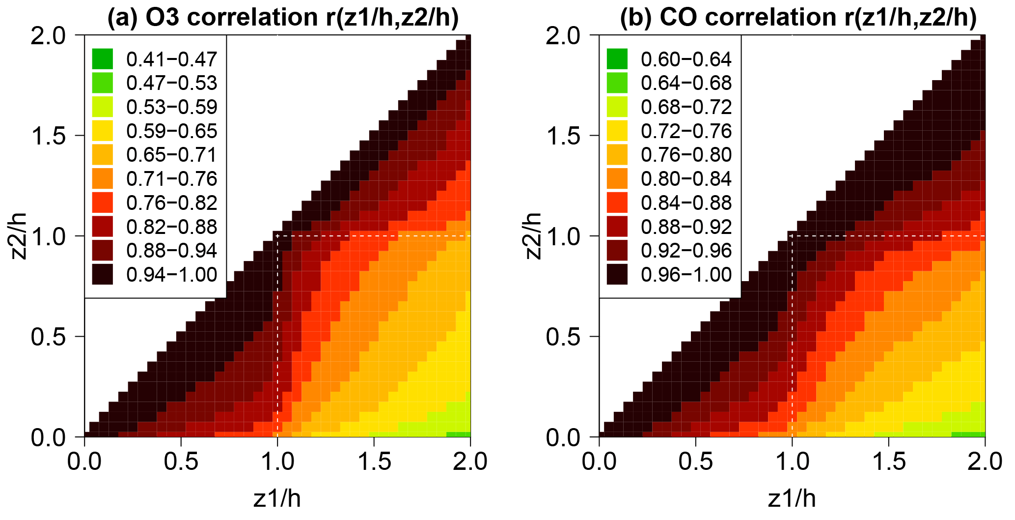
Figure 15Correlation of O3 (a) and CO (b) mixing ratios between the different z∕h altitude levels. All vertical profiles without any data gaps are taken into account. The correlation matrix is symmetric by construction.
4.4.3 Vertical autocorrelation
In this section, we analyse the vertical autocorrelation of O3 mixing ratios in the z∕h vertical coordinate system in order to further investigate the links between the PBL and the FT. The vertical autocorrelation designates the correlation of mixing ratios between two different altitude levels. Based on all individual profiles, we calculate the correlation (R) between the different pairs of z∕h altitude levels. The obtained O3 vertical autocorrelation matrix is shown in Fig. 15. The CO matrix is also shown for comparison. Results highlight a difference in variability apart from the PBL–FT interface. Indeed, within both the PBL (z∕h between 0 and 1) and FT (z∕h between 1 and 2), strong correlations are found, usually above 0.75. Conversely, correlations between the two atmospheric compartments are found to decrease more quickly with vertical distance, as illustrated by the (“wave”) shape of the iso-correlation contours. For instance, O3 mixing ratios at 0.9 (i.e. just below the PBL top) appear highly correlated with O3 mixing ratios in the entire PBL with correlations above 0.75 down to 0.0.5, but correlations are found to (more) quickly deteriorate with altitude in the FT, the 0.75 threshold being reached at 1.4. Similar results are found for CO, except that the change in correlation apart from the PBL–FT interface is slightly more smoothed compared to O3. This would be consistent with the fact that the differences in CO between the PBL and FT are mostly explained by the dynamics (transport) in contrast to O3, for which the chemistry prevailing within the PBL helps to differentiate the O3 mixing ratios and their variability more strongly in the two atmospheric compartments (as discussed in Sect. 4.4.1).
In this study, we investigated the vertical stratification of O3 and CO in the PBL and at the interface with the FT. Some results were also given for potential temperature and RH. We collected all the in situ vertical profiles measured by WOUDC ozonesondes and IAGOS aircraft at the northern mid-latitudes. Over the period 1994–2016, this represents a dataset of more than 90 000 profiles (78 % IAGOS profiles, 22 % sonde profiles).
As a preliminary step, we used all temperature profiles to identify surface-based and elevated temperature inversions (denoted SBIs and EIs, respectively). The occurrence of SBIs was found to strongly vary throughout the day, with frequencies ranging between 10 % at midday and 60 % in the very early morning. Our results also highlighted strong diurnal variations in the characteristics of SBIs, the deepest and strongest SBIs being observed during the night. However, no particular seasonal variation in SBIs was observed. On the profiles without SBIs, we looked for EIs, the base of which was taken as an estimate of the PBL height. This approach allows us to identify where the capping inversion occurs but this likely does not always correspond to the PBL height as it may sometimes correspond to the top of a residual layer (especially during the night or in the morning when the PBL is not fully developed). In contrast to SBIs, EIs exhibited no diurnal variations but some weak seasonal variations, with the deepest (thinnest) and sharpest (smoothest) EIs occurring during winter (summer); the strength is represented here by the temperature lapse rate within the inversion layer. The climatological PBL heights as determined with the EI method were found to be consistent with the results obtained by Seidel et al. (2010) through a more exhaustive analysis of meteorological sondes.
Based on these PBL height estimations (denoted h), we built the so-called PBL-referenced vertical distribution of RH, O3 and CO calculated by averaging all individual profiles formerly expressed as a function of z∕h (with z the altitude). Considering z∕h rather than z aims at shedding light on the features at the PBL–FT interface which would have been smoothed otherwise. For all meteorological parameters and chemical species, the PBL-referenced profiles highlighted clear inflexion points at the PBL top, which supports our ability to capture reasonably well a real geophysical interface with the EI method. Comparing the PBL-referenced profiles obtained with IAGOS and ozonesondes taken separately showed a broad consistency for potential temperature and RH, although some differences exist. In order to quantify how well pollutants are mixed within the PBL, we introduced two factors of vertical stratification, the first (γ) being defined as the standard deviation of the profile in the PBL (z∕h between 0 and 1) normalized by the mean and the second (δ) being defined as γ normalized by the PBL height. Results showed that the frequently assumed well-mixed PBL remains an exception. The γ (δ) vertical stratification of CO within the PBL was 11 % (1.7 % hm−1) on average, with some seasonal and diurnal variations (only for δ). A stronger vertical stratification was found for O3 with a γ (δ) factor of 18 % (5.1 % hm−1) on average. The seasonal and diurnal variations of the O3 vertical stratification were also stronger than for CO, with values ranging from ∼ 10 % in spring–summer midday–afternoon to ∼ 25 % in winter–fall night. For both species, this vertical stratification was not uniform through the PBL as stronger vertical gradients were found at both the surface (dry deposition and titration by NO for O3; surface emissions for CO) and the PBL–FT interface. These vertical gradients at the PBL top strongly vary with the season, with maximum (minimum) values in winter (summer). In comparison, lower vertical gradients were found in the lower FT. Investigating the variations of the vertical stratification factors with the surface potential temperature highlighted an interesting bell shape for O3 (but not for CO) with the weakest stratification at both the lowest (typically negative) and highest temperatures. This could be due to a substantial decrease in the O3 dry deposition in the presence of snow, although dedicated studies are required to confirm or reject this hypothesis. Consistent PBL-referenced profiles were obtained for IAGOS and ozonesondes taken separately.
Therefore, these results illustrate the fact that EIs indeed act as a geophysical interface between the PBL and FT. Compared to CO, the O3 PBL-referenced profiles exhibit a sharper inflexion point at the PBL–FT interface, which suggests that the CO inflexion point may be mostly due to dynamics (since its chemical reactivity is low), while the stronger O3 inflexion point would result from the combined effect of both dynamics and chemistry (different chemical regimes between the PBL and FT). This is also supported by the matrices of vertical autocorrelation that highlighted lower correlations apart from the PBL–FT interface and higher correlations within each of the two atmospheric compartments (PBL and FT), especially for O3.
This study focused on the general characteristics of the O3 and CO vertical stratification at northern mid-latitudes by aggregating the largest amount of profiles. It would be interesting in the near future to investigate how these PBL-referenced profiles differ depending on the environment (urban, rural, coastal, remote) or the region. In order to make some relevant comparisons, such an analysis would require a sufficiently large amount of data since O3 and CO profiles often exhibit both high variability and a complex vertical structure due to the numerous processes at work. Among the other perspectives, as they combine both chemical (mixing ratios) and dynamical (PBL height) information, these PBL-referenced profiles may offer a more meaningful way to evaluate the ability of CTMs to properly reproduce the vertical distribution of pollution in a constantly evolving PBL. Although current CTMs are probably not able to reproduce the sharp gradients in the capping inversion or entrainment zone due to too-coarse vertical resolution, it remains important to investigate more thoroughly how well they simulate the vertical distribution of the pollutants under varying PBL conditions. This is particularly important in urban areas where strong emissions occur at a surface characterized by a complex roughness (due to buildings), which greatly influences the pollution dispersion. As it operates multispecies (O3, CO, and now NOx, as well as CO2, CH4 and aerosols in the near future) profile measurements in the vicinity of large agglomerations, the IAGOS research infrastructure offers rich opportunities for such studies. In order to allow for further studies, the mean climatological O3 and CO PBL-referenced profiles analysed in this study are freely available on the IAGOS portal for each season and time of day (http://dx.doi.org/10.25326/4) (Petetin et al., 2018b). Concerning the representativeness of this dataset and the potential impact of airport pollution on IAGOS observations, an in-depth O3 and CO comparison between IAGOS and nearby and more distant surface stations around a few major European airports has recently shown that the IAGOS data in the lowest troposphere exhibit characteristics typical of urban–suburban surface stations (Petetin et al., 2018a). This should encourage more detailed model evaluations of the vertical distribution of the pollution, as now performed operationally with CAMS regional models in the framework of Copernicus (see http://www.iagos.fr/cams for daily comparisons).
No new measurements were made for this review article. All datasets mentioned in the text were obtained from existing databases. The IAGOS data are available at http://www.iagos.fr or directly via the AERIS website at http://www.aeris-data.fr. The ozone soundings can be downloaded from the World Ozone and Ultraviolet Radiation Data Centre (WOUDC) database (http://www.woudc.org) supported by Environment Canada (https://doi.org/10.14287/10000001, WMO/GAW Ozone Monitoring Community, 2018). The climatological O3 and CO PBL-referenced profiles are available through the IAGOS central database (http://iagos.sedoo.fr) and are part of the ancillary products (https://doi.org/10.25326/4) (Petetin et al., 2018b).
The supplement related to this article is available online at: https://doi.org/10.5194/acp-18-9561-2018-supplement.
Contributed to conception and design: HP.
Contributed to data acquisition:
HP, VT, BS, HC, GA, RB, DB, J-MC, SR,
PN, HGJS and PN.
Contributed to data analysis and interpretation:
HP, BS, HGJS, FG, FL and VT.
Drafted the article: HP.
Revised the article: HP, BS, VT, HC, RB, HGJS and FG.
The authors declare that they have no conflict of interest.
We acknowledge the strong support of the European Commission, Airbus and
the airlines (Lufthansa, Air France, Austrian Airlines, Air Namibia, Cathay Pacific,
Iberia and China Airlines so far) that carry the MOZAIC or IAGOS equipment
and have performed maintenance since 1994. In its last 10 years of operation,
MOZAIC has been funded by INSU-CNRS (France), Météo-France,
Université Paul Sabatier (Toulouse, France) and Research Center
Jülich (FZJ, Jülich, Germany). IAGOS has been additionally funded by
the EU projects IAGOS-DS and IAGOS-ERI. The MOZAIC–IAGOS database is
supported by AERIS (CNES and INSU-CNRS). We also acknowledge the WOUDC, the
WMO-GAW and all individual contributors for providing access to the
ozonesonde dataset. We thank the reviewers for their positive contributions
to this study.
Edited by: Aijun Ding
Reviewed by: two anonymous referees
Berkes, F., Neis, P., Schultz, M. G., Bundke, U., Rohs, S., Smit, H. G. J., Wahner, A., Konopka, P., Boulanger, D., Nédélec, P., Thouret, V., and Petzold, A.: In situ temperature measurements in the upper troposphere and lowermost stratosphere from 2 decades of IAGOS long-term routine observation, Atmos. Chem. Phys., 17, 12495–12508, https://doi.org/10.5194/acp-17-12495-2017, 2017.
Bian, J., Chen, H., Vömel, H., Duan, Y., Xuan, Y., and Lü, D.: Intercomparison of humidity and temperature sensors: GTS1, Vaisala RS80, and CFH, Adv. Atmos. Sci., 28, 139–146, https://doi.org/10.1007/s00376-010-9170-8, 2011.
Cohn, S. A. and Angevine, W. M.: Boundary Layer Height and Entrainment Zone Thickness Measured by Lidars and Wind-Profiling Radars, J. Appl. Meteorol., 39, 1233–1247, https://doi.org/10.1175/1520-0450(2000)039<1233:BLHAEZ>2.0.CO;2, 2000.
Colbeck, I. and Harrison, R. M.: Dry deposition of ozone: some measurements ofdeposition velocity and of vertical profiles to 100 metres, Atmos. Environ., 19, 1807–1818, https://doi.org/10.1016/0004-6981(85)90007-1, 1985.
Dupont, E., Menut, L., Carissimo, B., Pelon, J., and Flamant, P.: Comparison between the atmospheric boundary layer in Paris and its rural suburbs during the ECLAP experiment, Atmos. Environ., 33, 979–994, https://doi.org/10.1016/S1352-2310(98)00216-7, 1999.
Elguindi, N., Clark, H., Ordóñez, C., Thouret, V., Flemming, J., Stein, O., Huijnen, V., Moinat, P., Inness, A., Peuch, V.-H., Stohl, A., Turquety, S., Athier, G., Cammas, J.-P., and Schultz, M.: Current status of the ability of the GEMS/MACC models to reproduce the tropospheric CO vertical distribution as measured by MOZAIC, Geosci. Model Dev., 3, 501–518, https://doi.org/10.5194/gmd-3-501-2010, 2010.
Helmig, D., Ganzeveld, L., Butler, T., and Oltmans, S. J.: The role of ozone atmosphere-snow gas exchange on polar, boundary-layer tropospheric ozone – a review and sensitivity analysis, Atmos. Chem. Phys., 7, 15–30, https://doi.org/10.5194/acp-7-15-2007, 2007.
Helten, M., Smit, H. G. J., Sträter, W., Kley, D., Nedelec, P., Zöger, M., and Busen, R.: Calibration and performance of automatic compact instrumentation for the measurement of relative humidity from passenger aircraft, J. Geophys. Res.-Atmos., 103, 25643–25652, https://doi.org/10.1029/98JD00536, 1998.
Kaser, L., Patton, E. G., Pfister, G. G., Weinheimer, A. J., Montzka, D. D., Flocke, F., Thompson, A. M., Stauffer, R. M., and Halliday, H. S.: The effect of entrainment through atmospheric boundary layer growth on observed and modeled surface ozone in the Colorado Front Range, J. Geophys. Res.-Atmos., 122, 6075–6093, https://doi.org/10.1002/2016JD026245, 2017.
Lilly, D. K.: Entrainment into Mixed Layers. Part I: Sharp-Edged and Smoothed Tops, J. Atmos. Sci., 59, 3340–3352, https://doi.org/10.1175/1520-0469(2002)059<3340:EIMLPI>2.0.CO;2, 2002.
Lin, M., Fiore, A. M., Cooper, O. R., Horowitz, L. W., Langford, A. O., Levy, H., Johnson, B. J., Naik, V., Oltmans, S. J., and Senff, C. J.: Springtime high surface ozone events over the western United States: Quantifying the role of stratospheric intrusions, J. Geophys. Res.-Atmos., 117, D00V22, https://doi.org/10.1029/2012JD018151, 2012.
Lin, M., Fiore, A. M., Horowitz, L. W., Langford, A. O., Oltmans, S. J., Tarasick, D., and Rieder, H. E.: Climate variability modulates western US ozone air quality in spring via deep stratospheric intrusions, Nat. Commun., 6, 7105, https://doi.org/10.1038/ncomms8105, 2015.
Liu, S. and Liang, X.-Z.: Observed Diurnal Cycle Climatology of Planetary Boundary Layer Height, J. Climate, 23, 5790–5809, https://doi.org/10.1175/2010JCLI3552.1, 2010.
Marenco, A., Thouret, V., Nédélec, P., Smit, H., Helten, M., Kley, D., Karcher, F., Simon, P., Law, K., Pyle, J., Poschmann, G., Von Wrede, R., Hume, C. and Cook, T.: Measurement of ozone and water vapor by Airbus in-service aircraft: The MOZAIC airborne program, an overview, J. Geophys. Res.-Atmos., 103, 25631–25642, https://doi.org/10.1029/98JD00977, 1998.
Nédélec, P., Cammas, J.-P., Thouret, V., Athier, G., Cousin, J.-M., Legrand, C., Abonnel, C., Lecoeur, F., Cayez, G., and Marizy, C.: An improved infrared carbon monoxide analyser for routine measurements aboard commercial Airbus aircraft: technical validation and first scientific results of the MOZAIC III programme, Atmos. Chem. Phys., 3, 1551–1564, https://doi.org/10.5194/acp-3-1551-2003, 2003.
Nédélec, P., Blot, R., Boulanger, D., Athier, G., Cousin, J.-M., Gautron, B., Petzold, A., Volz-Thomas, A., and Thouret, V.: Instrumentation on commercial aircraft for monitoring the atmospheric composition on a global scale: the IAGOS system, technical overview of ozone and carbon monoxide measurements, Tellus B, 67, 1–16, https://doi.org/10.3402/tellusb.v67.27791, 2015.
Neis, P., Smit, H. G. J., Krämer, M., Spelten, N., and Petzold, A.: Evaluation of the MOZAIC Capacitive Hygrometer during the airborne field study CIRRUS-III, Atmos. Meas. Tech., 8, 1233–1243, https://doi.org/10.5194/amt-8-1233-2015, 2015a.
Neis, P., Smit, H. G. J., Rohs, S., Bundke, U., Krämer, M., Spelten, N., Ebert, V., Buchholz, B., Thomas, K., and Petzold, A.: Quality assessment of MOZAIC and IAGOS capacitive hygrometers: insights from airborne field studies, Tellus B, 67, 28320, https://doi.org/10.3402/tellusb.v67.28320, 2015b.
Petetin, H., Thouret, V., Athier, G., Blot, R., Boulanger, D., Cousin, J.-M., Gaudel, A., Nédélec, P., and Cooper, O.: Diurnal cycle of ozone throughout the troposphere over Frankfurt as measured by MOZAIC-IAGOS commercial aircraft, Elem. Sci. Anthr., 4, 1–11, https://doi.org/10.12952/journal.elementa.000129, 2016.
Petetin, H., Jeoffrion, M., Sauvage, B., Athier, G., Blot, R., Boulanger, D., Clark, H., Cousin, J.-M., Gheusi, F., Nedelec, P., Steinbacher, M., and Thouret, V.: Representativeness of the IAGOS airborne measurements in the lower troposphere, Elem. Sci. Anth., 6, 1–24, https://doi.org/10.1525/elementa.280, 2018a.
Petetin, H., Sauvage, B., and Boulanger, D.: IAGOS ancillary data: PBL-referenced profiles of O3 and CO, https://doi.org/10.25326/4, 2018b.
Petzold, A., Thouret, V., Gerbig, C., Zahn, A., Brenninkmeijer, C. A. M., Gallagher, M., Hermann, M., Pontaud, M., Ziereis, H., Boulanger, D., Marshall, J., Nédélec, P., Smit, H. G. J., Friess, U., Flaud, J.-M., Wahner, A., Cammas, J.-P., and Volz-Thomas, A.: Global-scale atmosphere monitoring by in-service aircraft – current achievements and future prospects of the European Research Infrastructure IAGOS, Tellus B, 67, 28452, https://doi.org/10.3402/tellusb.v67.28452, 2015.
Schröder, M., Lockhoff, M., Shi, L., August, T., Bennartz, R., Borbas, E., Brogniez, H., Calbet, X., Crewell, S., Eikenberg, S., Fell, F., Forsythe, J., Gambacorta, A., Graw, K., Ho, S.-P., Höschen, H., Kinzel, J., Kursinski, E. R., Reale, A., Roman, J., Scott, N., Steinke, S., Sun, B., Trent, T., Walther, A., Willen, U., and Yang, Q.: GEWEX water vapor assessment (G-VAP), WCRP Report 16/2017; World Climate Research Programme (WCRP): Geneva, Switzerland, 216 pp, 2017.
Seibert, P., Beyrich, F., Gryning, S.-E., Joffre, S., Rasmussen, A. and Tercier, P.: Review and intercomparison of operational methods for the determination of the mixing height, Atmos. Environ., 34, 1001–1027, https://doi.org/10.1016/S1352-2310(99)00349-0, 2000.
Seidel, D. J., Ao, C. O., and Li, K.: Estimating climatological planetary boundary layer heights from radiosonde observations: Comparison of methods and uncertainty analysis, J. Geophys. Res., 115, D16113, https://doi.org/10.1029/2009JD013680, 2010.
Smit, H. G. J., Rohs, S., Neis, P., Boulanger, D., Krämer, M., Wahner, A., and Petzold, A.: Technical Note: Reanalysis of upper troposphere humidity data from the MOZAIC programme for the period 1994 to 2009, Atmos. Chem. Phys., 14, 13241–13255, https://doi.org/10.5194/acp-14-13241-2014, 2014.
Solazzo, E., Bianconi, R., Pirovano, G., Moran, M. D., Vautard, R., Hogrefe, C., Appel, K. W., Matthias, V., Grossi, P., Bessagnet, B., Brandt, J., Chemel, C., Christensen, J. H., Forkel, R., Francis, X. V., Hansen, A. B., McKeen, S., Nopmongcol, U., Prank, M., Sartelet, K. N., Segers, A., Silver, J. D., Yarwood, G., Werhahn, J., Zhang, J., Rao, S. T., and Galmarini, S.: Evaluating the capability of regional-scale air quality models to capture the vertical distribution of pollutants, Geosci. Model Dev., 6, 791–818, https://doi.org/10.5194/gmd-6-791-2013, 2013.
Stocker, D. W., Zeller, K. F., and Stedman, D. H.: O3 and NO2 fluxes over snow measured by eddy correlation, Atmos. Environ., 29, 1299–1305, https://doi.org/10.1016/1352-2310(94)00337-K, 1995.
Stull, R. B.: An Introduction to Boundary Layer Meteorology, Kluwer Academic Publishers, Dordrecht, the Netherlands, 1988.
Thouret, V., Marenco, A., Logan, J. A., Nédélec, P., and Grouhel, C.: Comparisons of ozone measurements from the MOZAIC airborne program and the ozone sounding network at eight locations, J. Geophys. Res., 103, 25695–25720, https://doi.org/10.1029/98JD02243, 1998.
Travis, K. R., Jacob, D. J., Keller, C. A., Kuang, S., Lin, J., Newchurch, M. J., and Thompson, A. M.: Resolving ozone vertical gradients in air quality models, Atmos. Chem. Phys. Discuss., https://doi.org/10.5194/acp-2017-596, 2017.
Trousdell, J. F., Conley, S. A., Post, A., and Faloona, I. C.: Observing entrainment mixing, photochemical ozone production, and regional methane emissions by aircraft using a simple mixed-layer framework, Atmos. Chem. Phys., 16, 15433–15450, https://doi.org/10.5194/acp-16-15433-2016, 2016.
Vömel, H., Selkirk, H., Miloshevich, L., Valverde-Canossa, J., Valdés, J., Kyrö, E., Kivi, R., Stolz, W., Peng, G., and Diaz, J. A.: Radiation Dry Bias of the Vaisala RS92 Humidity Sensor, J. Atmos. Ocean. Tech., 24, 953–963, https://doi.org/10.1175/JTECH2019.1, 2007.
Wang, J., Zhang, L., Dai, A., Immler, F., Sommer, M., and Vömel, H.: Radiation Dry Bias Correction of Vaisala RS92 Humidity Data and Its Impacts on Historical Radiosonde Data, J. Atmos. Ocean. Tech., 30, 197–214, https://doi.org/10.1175/JTECH-D-12-00113.1, 2013.
Wang, X. Y. and Wang, K. C.: Estimation of atmospheric mixing layer height from radiosonde data, Atmos. Meas. Tech., 7, 1701–1709, https://doi.org/10.5194/amt-7-1701-2014, 2014.
Wesely, M. L., Cook, D. R., and Williams, R. M.: Field measurement of small ozone fluxes to snow, wet bare soil, and lake water, Bound.-Lay. Meteorol., 20, 459–471, https://doi.org/10.1007/BF00122295, 1981.
WMO: Quality Assurance and Quality Control for Ozonesonde Measurements in GAW – WMO Report No. 201, available at: https://www.wmo.int/pages/prog/arep/gaw/documents/GAW_201_30_Sept.pdf (last access: 22 March 2018), 2011.
WMO/GAW Ozone Monitoring Community: World Meteorological Organization-Global Atmosphere Watch Program (WMO-GAW)/World Ozone and Ultraviolet Radiation Data Centre (WOUDC) [Data], available at: https://doi.org/10.14287/10000001 (last access: 21 April 2017), 2018.