the Creative Commons Attribution 4.0 License.
the Creative Commons Attribution 4.0 License.
 | 04 Jul 2018
Future changes in surface ozone over the Mediterranean Basin in the framework of the Chemistry-Aerosol Mediterranean Experiment (ChArMEx)
Nizar Jaidan
Laaziz El Amraoui
Jean-Luc Attié
Philippe Ricaud
François Dulac
In the framework of the Chemistry-Aerosol Mediterranean Experiment (ChArMEx; http://charmex.lsce.ipsl.fr, last access: 22 June 2018) project, we study the evolution of surface ozone over the Mediterranean Basin (MB) with a focus on summertime over the time period 2000–2100, using the Atmospheric Chemistry and Climate Model Intercomparison Project (ACCMIP) outputs from 13 models. We consider three different periods (2000, 2030 and 2100) and the four Representative Concentration Pathways (RCP2.6, RCP4.5, RCP6.0 and RCP8.5) to study the changes in the future ozone and its budget. We use a statistical approach to compare and discuss the results of the models. We discuss the behavior of the models that simulate the surface ozone over the MB. The shape of the annual cycle of surface ozone simulated by ACCMIP models is similar to the annual cycle of the ozone observations, but the model values are biased high. For the summer, we found that most of the models overestimate surface ozone compared to observations over the most recent period (1990–2010). Compared to the reference period (2000), we found a net decrease in the ensemble mean surface ozone over the MB in 2030 (2100) for three RCPs: −14 % (−38 %) for RCP2.6, −9 % (−24 %) for RCP4.5 and −10 % (−29 %) for RCP6.0. The surface ozone decrease over the MB for these scenarios is much more pronounced than the relative changes of the global tropospheric ozone burden. This is mainly due to the reduction in ozone precursors and to the nitrogen oxide (NOx = NO + NO2)-limited regime over the MB. For RCP8.5, the ensemble mean surface ozone is almost constant over the MB from 2000 to 2100. We show how the future climate change and in particular the increase in methane concentrations can offset the benefits from the reduction in emissions of ozone precursors over the MB.
- Article
(5163 KB) - Full-text XML
- BibTeX
- EndNote


Several modeling studies have evaluated the future evolution of chemical and dynamical processes and have shown that future changes in ozone precursors have a significant impact on the evolution of tropospheric ozone and particularly surface ozone (e.g., West et al., 2007; Butler et al., 2012). Among the changes, the stratospheric influx increase is due, on one hand, to the global warming resulting from the accentuation of the residual atmospheric circulation forced by climate change (Collins et al., 2003; Sudo et al., 2003; Zeng et al., 2003; Butchart et al., 2006) and, on the other hand, to the recovery of stratospheric ozone (Zeng et al., 2010; Kawase et al., 2011). The abundance of ozone in the troposphere is controlled by various chemical and dynamical processes, sources such as chemical production, stratosphere–troposphere exchange (Danielsen, 1968), and sinks such as chemical destruction and dry deposition (Jacob, 2000). The magnitude of these processes depends on the abundance of ozone precursors, the extent of climate change and also the geographical location.
Tropospheric ozone is an air pollutant, an efficient greenhouse gas and also the primary source of hydroxyl radicals that control the oxidation capacity of the troposphere. It is produced by photochemical oxidation of methane (CH4), carbon monoxide (CO) and volatile organic compounds (VOCs) in the presence of nitrogen oxides (NOx = NO + NO2). Moreover, the efficiency of photochemical reactions forming ozone in the troposphere also depends on meteorological parameters such as temperature, radiation and precipitation (Jacob and Winner, 2009; Monks et al., 2015). At the surface, ozone is harmful to vegetation, materials and human health (Lippmann, 1989; Sandermann Jr., 1996; Brook et al., 2002; Fuhrer and Booker, 2003) even at relatively low concentrations (Bell et al., 2004). High ozone concentration is usually observed in the summer period because meteorological conditions (high temperatures, weak winds, low precipitation) favor photochemical ozone production (Meleux et al., 2007; Im et al., 2011).
The Mediterranean Basin (MB), surrounded by three continents with diverse pollution sources, is a region favoring the stagnation of pollutants, in particular during summer (Millán et al., 1996, 1997; Schicker et al., 2010). This region is sensitive to climate change (Giorgi, 2006) which is due to its particular location and diversity of ecosystems. Gerasopoulos et al. (2005) showed that transport from the European continent was identified as the main mechanism that controls ozone levels in the eastern MB. Akritidis et al. (2014) found significant negative ozone trends between 1996 and 2006 over the MB due to the reduction of ozone precursor emissions over continental Europe.
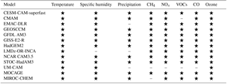
Table 1List of the historical ACCMIP simulations (2000 time slice) used in this study, and the availability of data for each model and parameter. “★” indicates “available”; “–” indicates “not available”.
A number of modeling studies have investigated the future changes of surface ozone due to climate change and ozone precursors evolution in Europe including the MB (Fiore et al., 2009; Wild et al., 2012; Langner et al., 2012; Colette et al., 2012). The chemical regime over the MB and southern Europe presents a pronounced NOx-limited regime (Beekmann and Vautard, 2010), except over maritime corridors and several major cities, e.g., Barcelona in Spain, Milan in Italy. In the NOx-limited regime with relatively low NOx and high VOCs, ozone decreases with NOx anthropogenic emission reductions and changes little in response to VOC anthropogenic emission reductions, and the reverse occurs in the VOC-limited regime (Sillman, 1995). A number of studies dealing with the future changes in surface ozone over the MB have been carried out at global and European scales. An assessment of the future changes in annual tropospheric ozone at global scale has been done by Young et al. (2013) using a set of chemistry models. At the regional scale, Lacressonnière et al. (2014) studied the future changes in surface ozone over Europe and the MB using a chemistry–transport model under the RCP8.5 scenario which corresponds to the pathway with the highest greenhouse gas emissions, leading to a radiative forcing of the order of 8.5 W m−2 at the end of the 21st century. The limited number of models and scenarios used in different studies increases the uncertainty and weakens the reliability of the results. In this paper, we analyze simulations performed from a set of chemistry models under four Representative Concentration Pathways (RCP2.6, RCP4.5, RCP6.0 and RCP8.5; Van Vuuren et al., 2011), defined in Sect. 2.1, to investigate the future changes in surface ozone over the MB, under a wide range of future projections. We highlight the impact of different factors contributing to surface ozone change: emissions, and meteorological and chemical parameters. This will also enable a better understanding of the effect of reducing ozone precursors on the future evolution of surface ozone.
In the framework of the Chemistry and Aerosol Mediterranean Experiment project (ChArMEx, http://charmex.lsce.ipsl.fr, last access: 22 June 2018), we focused on future changes in surface ozone from 2000 to 2100 above the MB using model outputs from the Atmospheric Chemistry and Climate Model Intercomparison Project (ACCMIP; Lamarque et al., 2013). This intercomparison project (ACCMIP) consists of a series of time slice experiments aiming at studying the long-term changes in atmospheric composition between 1850 and 2100. ACCMIP was designed to contribute to the Intergovernmental Panel on Climate Change (IPCC) Fifth Assessment Report (AR5) and analyses the driving forces of climate change in the simulations being performed in the fifth Coupled Model Intercomparison Project (CMIP5) (Taylor et al., 2012).
This paper is organized as follows. In Sect. 2, we provide a summary of the datasets used in this study, as well as the analysis approach. Section 3 focuses on the evaluation of the present-day (1990–2010) surface ozone simulations compared to independent observations. In Sect. 4, we explore the future changes in surface ozone for the periods 2030 and 2100 over the MB and discuss the various drivers affecting these changes such as meteorological parameters and ozone precursors. Conclusions are given in Sect. 5.
In this section, we provide some details about the ACCMIP models, the scenarios and the observations used in this study, followed by a general description of the analysis approach.
2.1 ACCMIP models and observations
We used the data from 13 models from the ACCMIP experiment. Note that model outputs are not available for all scenarios and periods (see Tables 1 and 2). The chemistry–transport model CICERO-OsloCTM2 was discarded in this study due to the absence of sufficient and required model outputs. Most of the models we used are chemistry–climate models (CCMs), except three models: MOCAGE (Modèle de Chimie Atmosphérique de Grande Echelle) which is a chemical transport model (CTM), using offline meteorological fields from an appropriate simulation of a climate model; STOC-HadAM3 (STOCHEM Lagrangian tropospheric chemistry–transport model coupled to the Hadley Centre atmospheric climate model); and UM-CAM (UK Met Office Unified Model version 4.5 combined with a detailed tropospheric chemistry scheme), referred to as chemistry general circulation models (CGCMs), which produce their own meteorological fields with no interaction with the concentrations of radiatively active species calculated by the chemistry scheme.
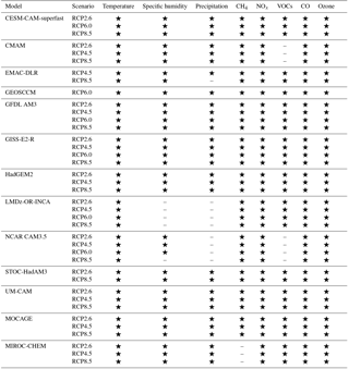
Table 2List of the future ACCMIP simulations used in this study and the availability of data for each model, parameter and scenario. “★” indicates “available” for the periods 2030 and 2100 except for GEOSCCM which is available only in 2100; “–” indicates “not available”.
A general evaluation and a detailed ACCMIP model description are provided in Lamarque et al. (2013). The models are driven by sea surface temperature (SST) and sea-ice concentrations (SICs). The complexity of chemical schemes varies considerably between models, from the simplified schemes of the CESM atmospheric chemistry–climate model (CESM-CAM-superfast) (16 species) to the more complex schemes of the GEOS chemistry–climate model (GEOSCCM) (120 species). The differences between models mostly come from the degree of representation of non-methane hydrocarbon (NMHC) emissions and chemistry in the models. The representation of stratospheric chemistry is included in the models, excepted in HadGEM2, LMDz-OR-INCA, STOC-HadAM3 and UM-CAM. LMDz-OR-INCA uses a constant (in time) stratospheric ozone climatology (Li and Shine, 1995), whereas the other models without detailed stratospheric chemistry use the time-varying stratospheric ozone dataset of Cionni et al. (2011). Iglesias-Suarez et al. (2016) evaluated the stratospheric ozone and associated climate impacts using the ACCMIP simulations in the recent past (1980–2000). They showed that ACCMIP multimodel mean total column ozone trends compare favorably against observations. They also demonstrated how changes in stratospheric ozone are intrinsically linked to climate changes. All anthropogenic and biomass burning emissions are specified for all models. However, the natural emissions are differently specified for the different models. In many cases, different models share several aspects such as dynamical cores, physical parameterizations, convection or the boundary layer scheme, but differ much in the number of chemical reactions. Consequently, all the models used in our study are considered distinct according to Lamarque et al. (2013).
A new set of future projections according to four scenarios called RCPs was released for CMIP5 (Moss et al., 2010). The RCPs are named according to the radiative forcing (RF) target level for 2100. The radiative forcing estimates are based on the forcing of long-lived and short-lived greenhouse gases and other forcing agents. The RCPs are four independent pathways developed by four separate Integrated Assessment Modeling (IAM) groups. The socioeconomics assumptions underlying each RCP are not unique; the four selected RCPs were considered to be representative of a larger set of scenarios in the literature and include one mitigation scenario leading to a very low forcing level (RCP2.6) which assumes a peak in RF at 3.0 W m−2 in the early 21st century before declining to 2.6 W m−2 in 2100 (Van Vuuren et al., 2006, 2007), two medium RF stabilization scenarios (RCP4.5; RCP6.0), which stabilize after 2100 at 4.5 W m−2 and 6.0 W m−2, respectively (Fujino et al., 2006; Smith and Wigley, 2006; Hijioka et al., 2008; Wise et al., 2009), and one very high baseline emission scenario (RCP8.5) which assumes an increasing RF even after 2100 (Riahi et al., 2007). In a first phase, ACCMIP historical simulations (Hist) were carried out covering the pre-industrial period to the present day (Lamarque et al., 2010). Second, ACCMIP simulations were performed based on a range of RCPs (Van Vuuren et al., 2011) to cover 21st century projections. Ozone precursor emissions from anthropogenic and biomass burning sources were taken from those compiled by Lamarque et al. (2010) for the Hist simulations, whereas emissions for different RCP simulations are described by Lamarque et al. (2013). The four RCPs include reductions and redistribution of ozone precursor emissions in future projections except for CH4. Natural emissions, such as CO and VOCs from vegetation and oceans, and NOx from soil and lightning, were determined by each model group. In this study, we use available surface ozone observations based on the gridded observations given by Sofen et al. (2016) in order to evaluate uncertainty related to model simulations. Sofen et al. (2016) built a consistent gridded dataset for the evaluation of chemical transport and chemistry–climate models from all publicly available surface ozone observations from online databases of the modern era: the World Meteorological Organization (WMO) Global Atmospheric Watch (GAW), Cooperative Programme for Monitoring and Evaluation of the Long-range Transmission of Air Pollutants in Europe (EMEP), European Environment Agency Air-Base (EEA), US Environmental Protection Agency Clean Air Status and Trends Network (US EPA CASTNET), US EPA Air Quality System (AQS) Environment Canada's Air and Precipitation Monitoring Network (CAPMoN), Canadian National Air Pollution Survey Program (NAPS) and Acid Deposition Monitoring Network in East Asia (EANET). The surface ozone data used at global scale are built from 2531 sites, mostly (97 %) located between 22 and 69∘ N mainly in North America and western Europe (Sofen et al., 2016). Data are averaged within a global grid of 2∘ × 2∘. We use averages from hourly ozone data on a monthly basis from 1990 to 2010.
2.2 Analysis approach
In this study, we analyze the present-day and future simulations performed by the ACCMIP models over the MB. The objective is to assess the surface ozone evolution in a context of climate change. We use the four scenarios (RCP2.6, RCP4.5, RCP6.0 and RCP8.5) and focus on three periods: a reference period (REF) which corresponds to the 2000 time slice from the historical scenario and two future short- and long-term periods, corresponding to the 2030 and the 2100 time slices, respectively. The number of years simulated for each time slice mostly varied between 4 and 16 years for each model (see Table 3). The number of scenarios available is between one (for GEOSCCM) and four (for LMDz-OR-INCA, GISS-E2-R, GFDL AM3 and NCAR CAM3.5) (see Table 2, which shows the available scenarios as well as the meteorological and chemical parameters for each model).
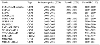
Table 3List of the ACCMIP model used in this study and the time slice availability for each model.
This study is composed of two parts. The first part consists of a model assessment based on the REF period, in which we compare the outputs of different models to a set of available surface ozone data based on the gridded observations given by Sofen et al. (2016). We use several statistical diagnostics to assess the performances of different model outputs. The individual model performances and the ACCMIP ensemble mean are compared to the averaged observations over the period 1990–2010. For the evaluation of the different models, we use a set of metrics (see Table 4), the correlation coefficient (R), the normalized mean biases (NMB), the mean bias (MnB), the mean absolute gross error (MAGE) and the root mean square error (RMSE). In addition to these metrics, we use two unbiased symmetric metrics introduced by Yu et al. (2006) that are found to be statistically robust and easier to interpret: the normalized mean bias factor (NMBF) and the normalized mean absolute error factor (NMAEF). The aim is to better understand the behavior of each model that simulates annual and summer surface ozone in recent conditions.
Table 4Definition of the metrics used to evaluate the ACCMIP model performances. O and M refer to observations and model, respectively. , .
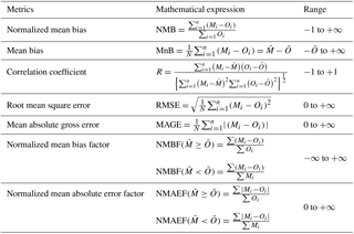
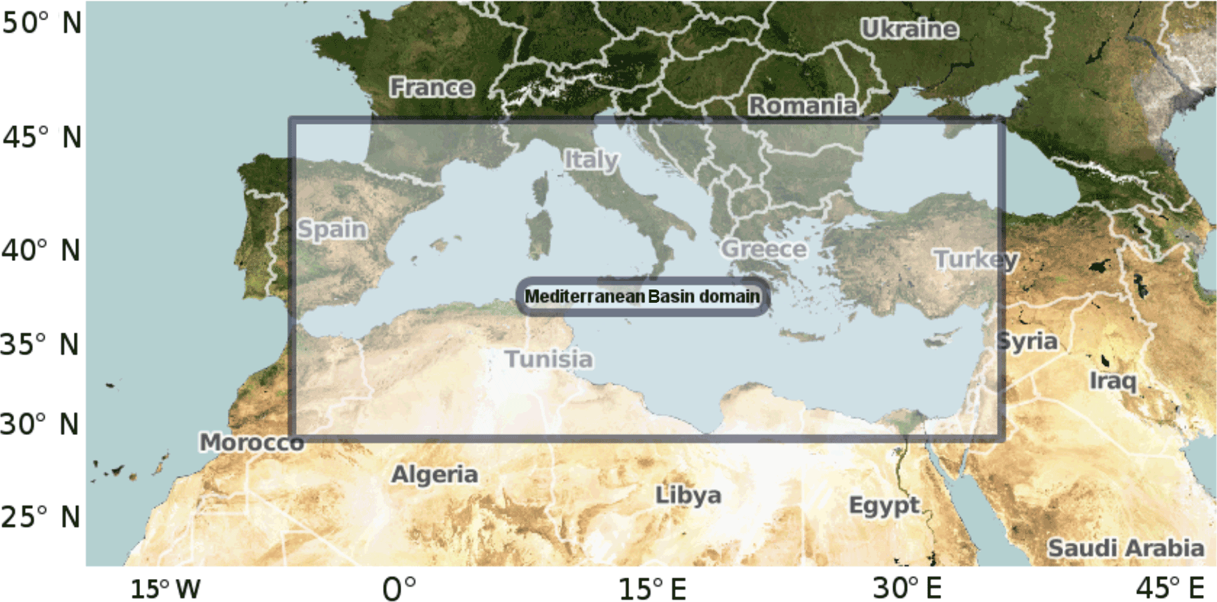
Figure 1The Mediterranean region including southern Europe, northern Africa and a part of the Middle East. The grey box represents the Mediterranean Basin (MB) domain, in which the statistical analysis is performed.
The second part is dedicated to the study of the future evolution of surface ozone in summer linked to meteorological variables (temperature, humidity and precipitation) and ozone precursors at the surface (CH4 concentration, CO, VOCs and NOx emissions). The study is focused on June, July and August (JJA), except for the investigation of the annual cycle of surface ozone over the MB (Sect. 3.1). We averaged the available output simulations in summertime (JJA) and over the box representing the MB domain included in the Mediterranean region (see Fig. 1). This future projection is compared to the REF period, using the box-and-whisker plots by specifying outliers with Tukey's fences rule (Tukey, 1977) of 1.5 times the interquartile range (outliers are values more than 1.5 times the interquartile range from the quartiles). In order to highlight the regions with a significant change in surface ozone, as well as to evaluate the statistical significance of our results, we use a field significance test (Benjamini and Hochberg, 1995; Wilks, 2006) that satisfied the false discovery rate (FDR) criterion with αFDR=0.10. The FDR method was performed using p values from a local Student t test that was computed for each grid point with 95 % confidence level. The future evolution of the ozone budget is also discussed.
Atmospheric Chemistry and Climate Model Intercomparison Project model simulations have been extensively evaluated on a global scale by Lamarque et al. (2013) and Young et al. (2013). In this paper, we study the behavior of each model that simulates surface ozone and we focus on the MB. We compare the REF ACCMIP simulations (see Table 1) to surface ozone observations based on the gridded observations given by Sofen et al. (2016). Note that the REF ACCMIP simulations are representative of the 2000 time slice and the surface ozone observations are averaged over the period 1990–2010. Our evaluation includes three parts: (1) evaluation of the annual cycle of surface ozone over the MB; (2) discussion and evaluation of the modeled ACCMIP mean surface ozone in summer; and (3) evaluation of models with a wide range of metrics and comparison of their performances between the regional and the global scales.
3.1 Annual cycle of surface ozone over the Mediterranean Basin
Figure 2a compares the annual cycle of surface ozone from the ACCMIP ensemble and the ACCMIP annual mean against gridded observations. This evaluation is carried out over the area in which observations are available. Most models are in agreement with the observed annual cycle showing a maximum in summer and a minimum in winter, except CESM-CAM-superfast, which shows a decrease in ozone during summer to reach a concentration equal to the observed surface ozone, and shows strong overestimations in other seasons. It should also be noted that the GEOSCCM, GISS-E2-R, the ECHAM/MESSy Atmospheric Chemistry (EMAC), HadGEM2 and LMDz-OR-INCA models show a maximum of ozone concentrations in August, in contrast to the observations that show a maximum in July. We also observe a general overestimation of the modeled surface ozone that is more pronounced in summer and particularly for GISS-E2-R, MOCAGE and STOC-HadAM3 with a positive mean bias of 13.33 to 24.34 ppbv (parts per billion by volume) compared to observations. The behavior of the annual cycle of surface ozone from ACCMIP models averaged over the period 1990–2010 over the Mediterranean Basin is quite similar to the one observed. The bias between the ACCMIP and the observed annual cycle is positive with values between 6.10 and 12.47 ppbv. The Canadian Middle Atmosphere Model (CMAM) model reproduces very well the annual cycle (Fig. 2a). Figure 2b shows the Taylor diagram (Taylor, 2001) which compares the annual cycle of surface ozone of different ACCMIP models to the averaged observation over the period 1990–2010. This diagram allows us to objectively compare the simulated and the observed annual cycles. In the Taylor diagram, the simulated patterns that agree the best with the observations should be close to the open circle marked “Obs” on the x axis (see Fig. 2b). The correlation coefficient (R) between simulated and observed annual cycles of surface ozone is generally greater than 0.75 for most of the models, except for LMDz-OR-INCA and CESM-CAM-superfast (). GISS-E2-R and GEOSCCM reach a correlation coefficient of 0.8. For the other models, the correlation coefficient exceeds 0.92. GEOSCCM, NCAR CAM3.5 and GFDL AM3 present a normalized standard deviation close to 1. The ACCMIP mean simulates very well the annual cycle shape of surface ozone and shows better performance than most of the other models, except GFDL AM3 and MIROC-CHEM, with a correlation coefficient of 0.93 and a normalized standard deviation of 0.87. In conclusion, most of the models are in agreement with the observations in terms of the annual cycle shape with a correlation coefficient greater than 0.8.
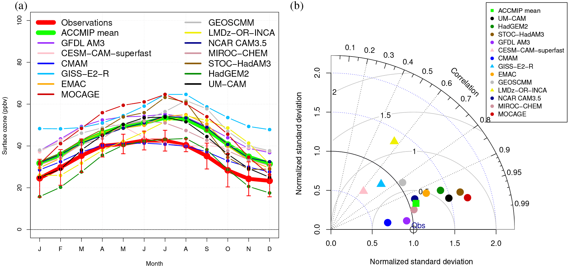
Figure 2(a) Annual cycle of surface ozone from ACCMIP models averaged over the period 1990–2010 and over the Mediterranean Basin (thin lines), between gridded observations (thick red line), ACCMIP ensemble mean (thick green line) and the ACCMIP ensemble. Error bars on the observations indicate interannual standard deviation. (b) Taylor diagram of the annual cycle of surface ozone averaged over the period 1990–2010. The radial coordinate shows the standard deviation, normalized by the observed standard deviation. The azimuthal variable shows the correlation of the modeled annual cycle with the observed annual cycle. The normalized root mean square error is indicated by the grey circle centered on the observational reference (Obs) point. Obs is indicated by the open circle on the x axis. The analysis is performed over the Mediterranean Basin domain (see Fig. 1). The different models and the observations are represented by a color as shown in the legends of each figure.
3.2 Modeled ACCMIP summer mean surface ozone
Figure 3a shows the ACCMIP multimodel ensemble mean of the summer surface ozone over the REF period. The general features, with higher ozone concentrations over the MB and the Middle East region, are observed, exceeding an average of 60 ppbv in the center of the MB. Over continental Europe and northern Africa, the ozone concentrations are smaller (≈ 40 ppbv) than over the MB. Several modeling studies have already shown this gradient in ozone concentration between land and sea (Lelieveld and Dentener, 2000; Zeng et al., 2008; Lacressonnière et al., 2012; Langner et al., 2012; Safieddine et al., 2014). A minimum in surface ozone is simulated over the northwestern Europe region, which corresponds to a VOC-limited regime in summertime, unlike the MB which is characterized by a NOx-limited regime as shown by Beekmann and Vautard (2010). This means that the ACCMIP ensemble mean respects the spatial variability of ozone related to the chemical regime. All models capture this variability in surface ozone concentrations (not shown).
Figure 3b shows the ACCMIP ensemble standard deviation (SD) of the summer surface ozone over the period 1990–2010. The different models are generally in agreement over the MB except over the Ligurian Sea (southern Po Valley, Italy, and around Marseille, France) with SD>13 ppbv. This region is characterized by a high density of anthropogenic and natural emissions (Silibello et al., 1998; Finzi et al., 2000; Martilli et al., 2002; Meleux et al., 2007). In the Po Valley, Vautard et al. (2007) show that the overestimation of simulated ozone concentrations is possibly due to the excessive stagnation of winds, and that the ability of models to simulate acute episodes is strongly variable in this region, explaining the difference between models.
Figure 4a shows the ACCMIP ensemble mean bias of the summer surface ozone over the period 1990–2010. Colored circles indicate the representative gridded observations. The black circles represent mainland and large islands labeled as “land”. The green circles represent maritime cell boxes and are mainly located over small islands labeled as “sea”. The ACCMIP ensemble mean overestimates surface ozone over the sea and central Europe. However, the ozone mean bias is negative in some regions in Spain and over one location (41∘ N, 19∘ E) where the observation concentration is up to 70 ppbv which is not reproduced by the models.
The ACCMIP ensemble mean of absolute error (Fig. 4b) shows an absolute error distribution similar to the distribution of the mean bias with a maximum absolute error of 12 ppbv over the central MB, central and Eastern Europe, and an absolute error of 7 ppbv over Crete and Cyprus.
Our study is consistent with various modeling studies showing a model overestimation of surface ozone observations at northern midlatitudes. Using most of the ACCMIP models, Young et al. (2013) suggest that the high bias in the Northern Hemisphere could indicate deficiencies with the ozone precursor emissions (see also, for different models, Goldberg et al., 2016 and Travis et al., 2016). Moreover, in a different experiment, Lin et al. (2008) suggest that the overestimation of models could also be due to an underestimation of ozone dry deposition velocity. In the same way, Ganzeveld et al. (2009) and Coleman et al. (2010) suggest that models are deficient in terms of dry deposition of gaseous species over oceans. Several other effects could be suggested, such as a high sensitivity of models to meteorological fields (Hu et al., 2017) or a combination of excessive vertical mixing and net ozone production in the model boundary layer (see Travis et al., 2016).
Schnell et al. (2015) evaluated a set of ACCMIP models against hourly surface ozone from 4217 ground-based stations in North America and Europe. They found that models are generally biased high during all hours of the day and in all regions. However, they also found that most models well simulate the shape of regional summertime diurnal and annual cycles. They concluded that the skill of the ACCMIP models provides confidence in their projections of future surface ozone.

Figure 3ACCMIP ensemble mean of surface ozone concentration in ppbv (a) and the ACCMIP ensemble standard deviation in ppbv (b) over the REF period (2000 time slice) from the historical experiment over the Mediterranean Basin. Red colors represent relatively high surface ozone concentration and large inter-model standard deviation for panels (a) and (b), respectively. Blue colors represent relatively low surface ozone concentration and small inter-model standard deviation for panels (a) and (b), respectively.
3.3 Model evaluation using metrics
A comparison of tropospheric ozone between ACCMIP models and observations from ozonesondes and spaceborne instruments is provided by Young et al. (2013). It shows that the ACCMIP ensemble performances to simulate tropospheric ozone vary between different regions over the world.
In our study, we use the ACCMIP simulations of surface ozone over a specific region, namely over the MB, but we compare the performances of the models at the regional MB and global scales. Figure 5 shows the ACCMIP model performance terms of MnB, MAGE, RMSE, NMBF and NMAEF, based on spatiotemporal (annual cycle) comparison of surface ozone between ACCMIP model simulations and averaged observations over the REF period. Rows and columns represent individual models and metrics, respectively. Each cell contains the value of a corresponding metric and a color indicating the performance of the model, from white (the closest to the observations) to red (the farthest from the observations). Each metric is calculated at the regional MB and global scales. Comparing the two colored tables (Fig. 5), we note that the color distribution is on average similar. This means that there is no significant difference in the model performances regarding the scale (global vs. regional MB), except for GEOSCCM and MOCAGE, whose performances are better at global than at regional scale. Note that EMAC, GEOSCCM, MOCAGE and CESM-CAM-superfast have a higher bias and error at the regional MB scale, particularly for GEOSCCM with a NMBF and a NMAEF of 0.49 and 0.51 against 0.32 and 0.35 at the global scale, respectively, unlike for the other models that have a slightly better score at the regional MB scale. GISS-E2-R is the farthest model from the observations with a NMBF and a NMAEF greater than 0.68 over the MB. The closest model to observations is CMAM with a NMBF close to zero and a NMAEF less than 0.24. Note that the CMAM model has a simplified chemical scheme (no NMVOCs). This may reduce uncertainties related to VOC emissions.
In conclusion, this evaluation shows that the models are different in terms of performances and most of the models overestimate the surface ozone. The bias is positive at the regional and the global scales for all models except HadGEM2. The model performances do not significantly change on average from the global to the regional scale (MB) over the REF period. Quantifying model uncertainty by comparison with observations in the recent past will help us to estimate their accuracy in the future projections.

Figure 4ACCMIP ensemble mean bias of surface ozone concentration in ppbv (a) and the ACCMIP ensemble mean error in ppbv (b) over the REF period (2000 time slice) from the historical experiment over the Mediterranean Basin. Black and green filled circles represent land and sea, respectively. Brown colors represent positive values of mean bias for panel (a) and red colors represent relatively large absolute error for panel (b). Blue colors represent negative values of mean bias for panel (a) and relatively small absolute error for panel (b).
In this section, we study the future changes in surface ozone and its budget over the MB in 2030 and 2100 compared to 2000. We also discuss the factors that could impact future trends in surface ozone: meteorological variables (temperature, specific humidity and precipitation), ozone precursors at the surface (CH4 concentration, CO, VOCs and NOx emissions) and future climate change. We use all available data from the 13 ACCMIP models (see Table 2) which have been evaluated in Sect. 3. Our study focuses mainly on the ACCMIP ensemble mean, which is representative of the ACCMIP ensemble (found to be close to observations). The future changes in surface ozone, ozone precursors and meteorological variables are averaged over the domain shown in Fig. 1. The entire study is focused on June, July and August (JJA) to be representative of the summer conditions. In this section, we will also discuss the results obtained.
4.1 Future changes in meteorological parameters
For each of the four RCPs, Fig. 6 shows the mean change in meteorological parameters from the ACCMIP models over the MB for the JJA period in 2000, 2030 and 2100. The number of available models for each period varies according to the different scenarios, but it is the same between 2030 and 2100 for each scenario except for RCP6.0 with one more model (GEOSCCM) in 2100 compared to the 2030 simulations (see Table 2).
The general trend in temperature from 2000 to 2100 is increasing (Fig. 6a), and the amplitude depends on the scenario and the period. An increase in temperature of 0.9–1.6 and 0.3–4.5 K is noted for the period 2000–2030 and 2030–2100, respectively. This increase depends linearly on the radiative forcing. We note that CESM-CAM-superfast shows a strong maximum in temperature in RCP8.5. Inter-model variability grows as a function of the increase in RF and is generally greater for 2100 than for 2030. Temperature increases on average by about 1.5 K for RCP2.6 and by 6.0 K for RCP8.5, between 2000 and 2100. In general, an increase in temperature favors biogenic emissions (mainly isoprene, a biogenic precursor of ozone) and favors photochemical reactions (Derwent et al., 2003).
In addition, the general trends in specific humidity (Fig. 6b) and temperature are similar. This can be interpreted as a result of evaporation, knowing that the MB will be affected by climate change and particularly exposed to high temperatures. The NCAR CAM3.5 is an outlier in terms of specific humidity. It presents a decrease in the specific humidity between 2030 and 2100 for RCP4.5 unlike the other models. Inter-model variability is greater for RCP2.6 and RCP6.0 than for the other scenarios, which is likely due to the uncertainty in the temperature change for RCP2.6 and perturbation due to the GEOSCCM model, which shows a minimum of humidity in 2100 for RCP6.0. Spivakovsky et al. (2000) showed that humidity is the most important meteorological factor affecting the lifetimes of OH and CH4 which are involved in the chemical production of ozone. More specifically, the increased humidity causes an ozone destruction which leads to a decrease in surface ozone.
In general, precipitation decreases for all RCPs except for RCP2.6 (Fig. 6c), and the decrease is more pronounced for RCP6.0 and RCP8.5. Precipitation from MOCAGE was ignored due to the high precipitation values (likely due to high convective precipitation) compared to other models.
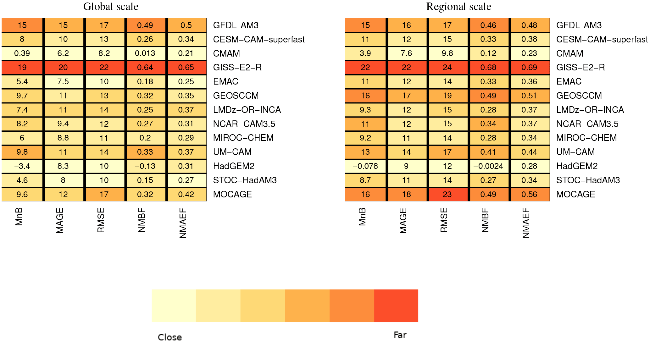
Figure 5ACCMIP model performances, based on spatiotemporal (annual cycle) comparison of summer surface ozone between observations and ACCMIP models computed over a REF period (1990–2010) from the historical experiment. Rows and columns represent individual models and metrics, respectively. Each cell contains the value of a corresponding metric and a color indicating the performance of the model, from white (close to the observations) to red (far from the observations). The metrics used are mean bias (MnB), mean absolute gross error (MAGE), root mean square error (RMSE), the normalized mean bias factor (NMBF) and the normalized mean absolute error factor (NMAEF). Each metric is calculated at global (left) and regional scales (right). The colors associated with each metric value were determined as follows: the values of each metric have been rescaled between 0 and 1 corresponding to the model that is close to and far from the observations, respectively. The interval [0,1] has been subdivided into six equal intervals, each representing a different color. The value of each metric is given by the color of the interval to which the rescaled value belongs.
To summarize, the ACCMIP mean surface temperature increases during the 21st century for the four RCPs, according to the radiative forcing. The surface specific humidity increases over the MB as a response to the rise in surface temperature and precipitation decreases for scenarios that have the highest RF (RCP6.0 and RCP8.5).
4.2 Future changes in ozone precursors
One of the strong assets of the ACCMIP experiment is that ozone precursors have been specified for all models. However, the biogenic emissions were not specified. Their estimates depend on each modeling group and, in addition to differences in model complexity and parameterizations, this can increase the inter-model variability. Figure 7 shows the mean change in ozone precursors (surface CH4 concentration, VOCs, CO and NOx emissions) in the ACCMIP models averaged over the MB over the JJA period of 2000, 2030 and 2100 time slices. The methane concentration at the surface decreases over the MB (Fig. 7a) between 2000 and 2030 by 10 % for RCP2.6 and increases for RCP4.5, RCP6.0 and RCP8.5 by 6, 6 and 27 %, respectively. Conversely, between 2030 and 2100, the average concentration of CH4 at the surface over the MB decreases by 21, 12 and 6 % for RCP2.6, RCP4.5 and RCP6.0, respectively. However, in the same period for RCP8.5, surface CH4 concentration increases by 73 %. Inter-model variability of CH4 is small relative to the total change for all RCPs. We also note that the total change in CH4 concentration over the MB is almost the same between RCP4.5 and RCP6.0, despite a significant difference in RF mainly due to the difference in the concentration of CO2 between these two scenarios. This is important in the interpretation of the difference in the surface ozone concentration between RCP4.5 and RCP6.0, knowing that long-term change in CH4 induces changes in ozone (West et al., 2007). The maximum and minimum CH4 concentrations observed in the four scenarios come from GISS-E2-R and LMDz-OR-INCA, respectively, and can be considered as outliers according to Tukey's fences rule. These two models are the only ones that do not prescribe CH4 concentrations in RCP simulations (Young et al., 2013).

Figure 6Box-and-whisker plots of the summer (JJA) average of (a) temperature in Kelvin (K), (b) specific humidity and (c) precipitation since 2000, calculated over the Mediterranean Basin domain (see Fig. 1) for the JJA period and for RCP2.6 (yellow), RCP4.5 (green), RCP6.0 (blue) and RCP8.5 (red). The historical period, considered as the reference, is in grey. The median is indicated by a horizontal black solid line and the multimodel mean by a filled black diamond. The range (25–75 %) is represented by the length of each colored box and the minimum/maximum (excluding outliers) by the whisker. Each filled circle represents a single model.
Figure 7b presents the evolution of total VOC emissions between 2000 and 2100. We note that the inter-model variability is high. This is mainly due to two factors. (1) The VOC module is different from one model to another. In other words, some models have more VOC species than others, and especially isoprene is not included in a few models (CMAM and HadGEM2). (2) The second factor is that the biogenic emissions are not specified in the ACCMIP experiment (but are included in most of the models). VOC emissions are mainly from biogenic origin, which explains this difference (Lamarque et al., 2013; Young et al., 2013). The multimodel average of VOCs decreases from 2000 to 2100 for all RCPs, but these changes are not significant given the very large inter-model variability. Note that there is a considerable variability in the complexity of the chemical schemes, in particular for the VOC schemes between the ACCMIP models.
Multimodel average of CO (Fig. 7c) decreases from 2000 to 2100 for all the RCPs, by 60, 58, 64 and 72 % for RCP2.6, RCP4.5, RCP6.0 and RCP8.5, respectively. This reflects the pollutant reduction policy that was implemented for the four scenarios in the IAM (Van Vuuren et al., 2011). The inter-model variability is relatively high, likely due to the difference between models in the representation of natural emissions from vegetation and ocean as well as in the complexity of their chemical schemes (for example, some models just include more CO to compensate missing NMVOCs). Outliers are HadGEM2 for RCP2.6, RCP4.5, RCP8.5 and GEOSCCM for RCP6.0, which correspond to a maximum of CO emission.
Figure 7d shows that NOx emissions generally decrease for the four RCPs. This decrease from 2000 to 2100 is more pronounced for RCP2.6 and RCP6.0 by 64 and 70 %, respectively, than for RCP4.5 and RCP8.5 by 47 and 37 %, respectively. In addition, the inter-model variability is relatively small. HadGEM2 is an outlier, representing the maximum of concentration in RCP2.6, RCP4.5 and RCP8.5. Other outliers are CESM-CAM-superfast for RCP8.5 (2030), EMAC for RCP4.5 (2100) and MIROC-CHEM for RCP2.6, RCP4.5 and RCP8.5. NCAR CAM3.5 and GFDL AM3 represent the minimum for RCP2.6. We identified outlier models which can adversely affect the quality of our results, but in terms of the future evolution, all models have similar trends.
In conclusion, the emissions of CO and NOx decrease linearly during the 21st century for the four RCPs, reflecting the emission reduction policy. The change in VOCs is not significant given the inter-model variability. The surface CH4 concentration increases between 2000 and 2030 by 6, 6 and 27 % for RCP4.5, RCP6.0 and RCP8.5, respectively, and decreases by 10 % for RCP2.6. However, the surface CH4 concentration increases by 73 % for RCP8.5 between 2030 and 2100 and decreases for the other scenarios over the same period.
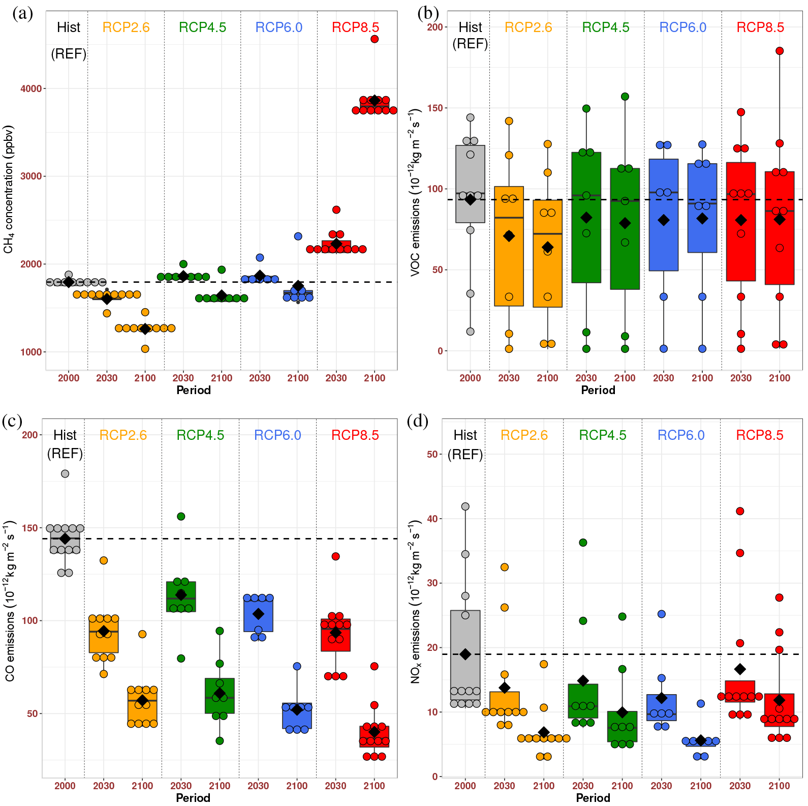
Figure 7Same as Fig. 6 but for (a) the surface CH4 concentrations and emissions of ozone precursors: (b) VOCs, (c) CO and (d) NOx.
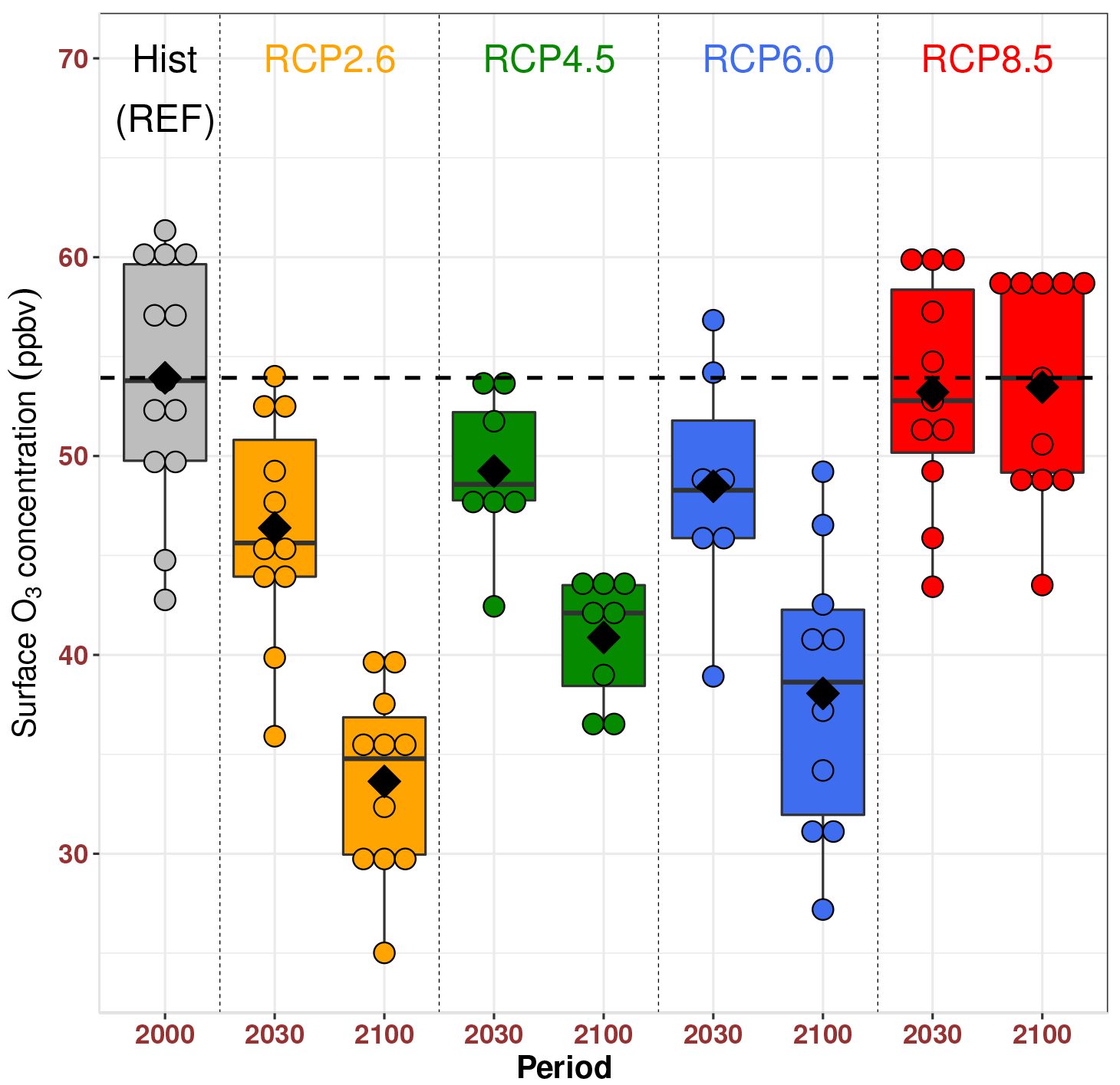
4.3 Future changes in surface ozone
Figure 8 shows the mean change in summer surface ozone between 2000 and 2100 over the MB. Compared to 2000, the relative changes for the summer surface ozone over the MB domain (see Fig. 1) in 2030 (2100) for the different RCPs are −14 % (−38 %) for RCP2.6, −9 % (−24 %) for RCP4.5, −10 % (−29 %) for RCP6.0 and −1.3 % (−0.8 %) for RCP8.5. The models with the most pronounced decrease are GISS-E2-R, GFDL AM3 and NCAR CAM3.5. Note that these models are biased high compared to the observations as seen in Sect. 3.3 (Fig. 5). However, the models are generally in agreement in terms of ozone future decrease between 2000 and 2100, except for RCP8.5. Young et al. (2013) show that the relative changes for the global tropospheric ozone burden in 2030 (2100) are −4 % (−16 %) for RCP2.6, 2 % (−7 %) for RCP4.5, 1 % (−9 %) for RCP6.0 and 7 % (18 %) for RCP8.5. The differences between changes in the summer surface ozone over the MB and changes in the tropospheric ozone burden reflect the fact that the surface ozone over the MB is mainly controlled by reductions in precursor emissions and the NOx-limited regime over the MB.
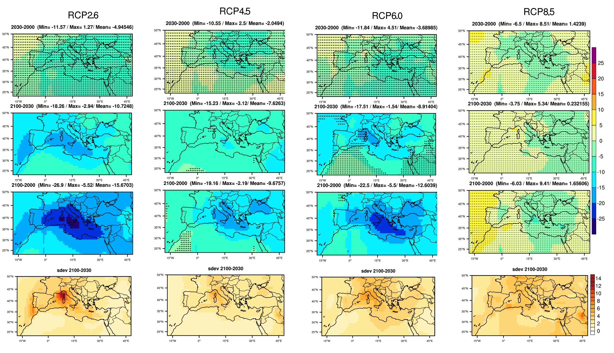
Figure 9ACCMIP ensemble mean surface ozone change (first to third rows) and standard deviation in ppbv (fourth row) between 2000 and 2100. Each column represents a Representative Concentration Pathway scenario. The rows from top to bottom correspond to anomalies in surface ozone concentration: REF–2030, 2030–2100, REF–2100 and the standard deviation of anomalies 2030–2100, respectively. REF represents the 2000 situation. Black dots indicate regions in the maps with statistically non-significant changes using a field significance test that satisfied the false discovery rate (FDR) criterion with αFDR=0.10. For the first to third rows, red and blue colors represent positive and negative trends, respectively. For the fourth row, red colors represent relatively large standard deviation and white colors represent relatively small standard deviation.
Figure 9 shows the surface ozone change between 2000 (REF) and 2030, 2030 and 2100, and 2000 and 2100. The ACCMIP models' ensemble mean differences and their standard deviation are calculated for the period 2000–2100 over the Mediterranean region (see Fig. 1) and for the four RCPs. In addition, we use a field significance test with a FDR criterion (αFDR=0.10) to have an idea about the statistical significance of surface ozone changes over the Mediterranean region. For RCP2.6, the surface ozone mean decreases between 2000 and 2030 over the Mediterranean region (−5 ppbv), with a minimum in southern Europe mainly in Italy (−11 ppbv). An increase is observed in the northwest of Europe (+ ppbv). However, over the period 2030–2100, the surface ozone decreases significantly over the Mediterranean region (−11 ppbv) and specifically over the Mediterranean Sea and the eastern part of the Atlantic Ocean (−18 ppbv). Over the period 2000–2100, the surface ozone decreases significantly on average by −16 ppbv. For RCP4.5, from 2000 to 2030, the ozone decrease is restricted to Europe and the Mediterranean Sea with an ozone increase over north Africa and the eastern part of the Atlantic Ocean, reaching a maximum of +2.5 ppbv unlike RCP2.6. Surface ozone remains generally constant over the Mediterranean area (−2 ppbv). However, a significant reduction in ozone occurs between 2030 and 2100 over the Mediterranean region (−8 ppbv) and specifically over the Mediterranean Sea and the Middle East (−15 ppbv). For RCP6.0 as for RCP2.6, the surface ozone decreases over the Mediterranean region between 2000 and 2100, reaching −22 ppbv over the Mediterranean Sea. Despite the large radiative effect that characterizes the RCP6.0 scenario, we observe a net decrease in the surface ozone concentration as for RCP2.6 and even more pronounced than RCP4.5. For the three scenarios, the surface ozone change is likely due to the decrease in ozone precursors (NOx, CH4 and CO) and also to the NOx-limited regime over the MB that connects ozone and its precursors. This means that ozone decreases with NOx emission reductions. We note that the changes in surface ozone are not statistically significant between 2000 and 2030.
Water vapor is also one of the most important climate variables affecting tropospheric ozone (Jacob and Winner, 2009). High values of specific humidity are simulated over the Mediterranean Sea due to evaporation (not shown). That can explain the largest decrease in surface ozone over the Mediterranean Sea and the eastern part of the Atlantic Ocean. The RCP8.5 is the only scenario that shows a very strong increase in CH4, temperature and specific humidity as seen previously in Figs. 6 and 7. These changes can be interpreted as a consequence of an intense climate change, despite the emission reduction policy and the chemical regime that promote the decrease in surface ozone.
For RCP8.5, from 2000 to 2030, surface ozone generally increases over the Mediterranean region (+1.5 ppbv) with a strong increase over the Arabian Peninsula (+9 ppbv) and a local decrease in southern Europe reaching −6 ppbv. The trend in surface ozone is the opposite: from +9 to −3 ppbv between 2030 and 2100 over the Middle East. The surface ozone increases between 2000 and 2100, except in southern Europe and the eastern part of the Mediterranean Sea. Note that the ACCMIP mean change in surface ozone, between 2030 and 2100, shows a marked east–west gradient with an increase in the west and a decrease in the east. This east–west gradient is represented by most of individual models (not shown). However, all the changes in surface ozone are not statistically significant for RCP8.5. Note that CMAM and HadGEM2 are the only models that show an increase over the entire Mediterranean region between 2000 and 2100. The inter-model standard deviation (SD) between 2030 and 2100 (Fig. 9 bottom) is generally small with SD<6 ppbv for the four scenarios, except for RCP2.6 over the Ligurian Sea (SD>10 ppbv), where some models provide a high concentration of ozone (e.g., GISS-E2-R). The disagreement between models over this region is highlighted in Sect. 3.2.
In conclusion, we show that surface ozone decreases between 2000 and 2100 for RCP2.6, RCP4.5, RCP6.0 and that the relative changes for the surface ozone over the MB decrease much more than the relative changes for the tropospheric ozone burden. For RCP8.5, the surface ozone remains constant between 2000 and 2100 over the MB. The decrease in surface ozone is more pronounced for RCP2.6 (−38 %) and RCP6.0 (−29 %) than that for RCP4.5 (−24 %), which is mainly due to the reduction of ozone precursors. The largest decrease is observed over the Mediterranean Sea and the eastern part of the Atlantic Ocean. For RCP8.5, the ACCMIP mean change in surface ozone between 2030 and 2100 shows a marked east–west gradient with an increase in the west and a decrease in the east, but these changes are not statistically significant.
4.4 Effects of ozone precursors on future surface ozone in the context of climate change
The future climate change is expected to influence the evolution of surface ozone through changes in temperature, solar radiation and water vapor (Meleux et al., 2007; Forkel Knoche, 2007; Hedegaard et al., 2008, 2013; Jacob and Winner, 2009; Katragkou et al., 2011; Lei et al., 2012; Doherty et al., 2013). This evolution of surface ozone may also be influenced by the increased Brewer–Dobson circulation which enhances the stratospheric contribution (Butchart and Scaife, 2001; Collins et al., 2003; Kawase et al., 2011; Lacressonnière et al., 2014). In addition, the impact of these climatic processes can be more marked over the MB. The Mediterranean Basin is directly under the descending branch of the Hadley circulation which is driven by deep convection in the Intertropical Convergence Zone (Lelieveld et al., 2002). The surface ozone changes are also controlled by changes in ozone precursor emissions and methane concentration. Several studies have highlighted the importance of CH4 emission control on surface ozone (e.g., Fiore et al., 2008; Wild et al., 2012).
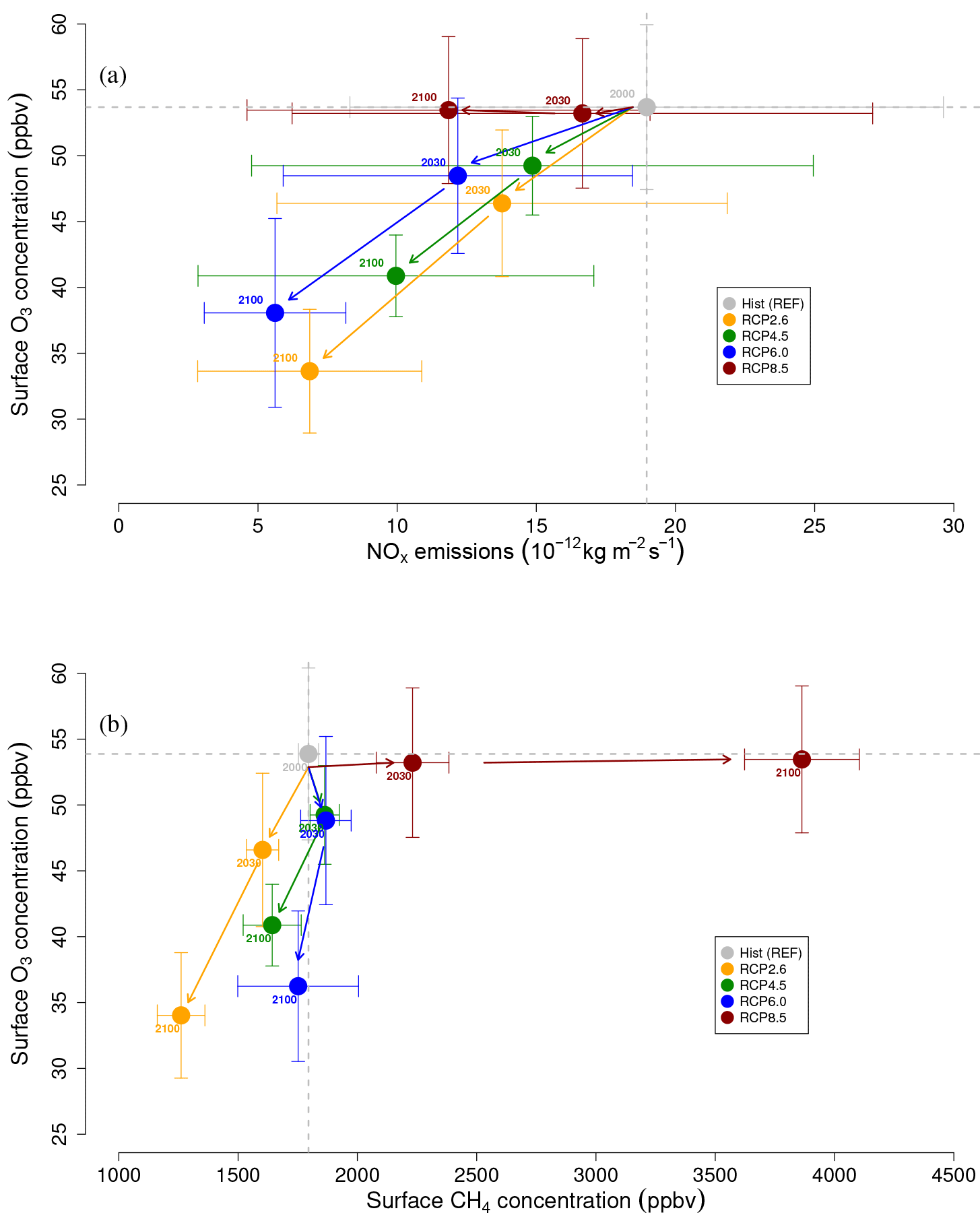
Figure 10ACCMIP model ensemble mean change in the surface ozone (ppbv) as a function of (a) changes in total NOx emissions (10−12 Kg m−2 s−1) and (b) changes in the surface CH4 concentration (ppbv), calculated over the Mediterranean Basin domain (see Fig. 1) for the JJA period and for the RCP2.6 (yellow), RCP4.5 (green), RCP6.0 (blue) and RCP8.5 (red) inset boxes. Error bars indicate multimodel standard deviation. Dashed lines refer to REF values (2000 time slice).
Figure 10 shows the surface ozone over the period from 2000 to 2100 as a function of the evolution of NOx emissions (Fig. 10a) and CH4 concentration (Fig. 10b). The relationship between ozone and NOx (Fig. 10a) is quasi-linear for RCP2.6, RCP4.5 and RCP6.0. A small decrease in NOx emissions implies a small decline in surface ozone as for RCP4.5 and a large decrease in NOx leads to a more pronounced decrease in ozone as for RCP2.6 and RCP6.0. Young et al. (2013) showed the same linear relationship by comparing the NOx emissions and the global modeled tropospheric ozone burdens, but with a smaller decrease in tropospheric ozone as seen in Sect. 4.3. However, for RCP8.5 scenario, the linear relationship between the two variables (NOx emissions and surface ozone) is no longer valid. Despite the decrease in NOx emissions, surface ozone remains constant for 2030 as for 2100.
The changes in CH4 concentration have no apparent impact on the changes in surface ozone for RCP2.6, RCP4.5 and RCP6.0 (Fig. 10b). Even if the CH4 concentration decreases (RCP2.6) or remains constant (RCP6.0), the surface ozone decline is similar in magnitude for the two scenarios. The RCP8.5 is marked by a nearly double increase in CH4 concentration, which is associated with a statistically non-significant change in surface ozone. This shows that the increase in CH4 is a contributing factor to the behavior change in the surface ozone evolution. Therefore, it can be deduced for RCP8.5 that a warmer climate associated with a strong increase in CH4 concentration will offset the benefit of the emission reductions. Wild et al. (2012) showed that 75 % of the average difference (5 ppbv) in surface ozone between the outlying RCP2.6 and RCP8.5 scenarios could be attributed to differences in CH4 abundance. We note that, for RCP8.5, the relative changes in summer surface ozone in 2030 (2100) over the MB are less intense with values of −1.3 % (−0.8 %) than for the global tropospheric ozone change with values of 7 % (18 %). This global tropospheric ozone change has already been highlighted by Young et al. (2013).
The different RCPs, implemented by independent modeling groups, are based on different radiative forcing levels (Moss et al., 2010). This makes the interpretation of our results regarding the different RCPs more complicated. Nevertheless, the comparison of scenarios can then be used to give a partial interpretation of the effect of climate change and in particular CH4 changes on surface ozone evolution. The magnitudes of the changes in temperature, specific humidity and CH4 concentrations are different for RCP2.6, RCP4.5 and RCP6.0. We note that the ozone evolutions are almost the same for these scenarios over the period 2000–2100, despite the marked difference in the global radiative forcing of 3.4 W m−2 which is mainly dominated by the forcing from CO2 (Van Vuuren et al., 2011). RCP6.0 can be considered as a scenario that could significantly decrease the future surface ozone over the MB. The beneficial effects of climate change through the increase of specific humidity due to the increase of temperature (Jacob and Winner, 2009) and the reduction policy of ozone precursors play an important role for the changes in surface ozone. For RCP8.5 scenario, the surface ozone over the MB remains constant over the period 2000–2100 with a strong increase in temperature, specific humidity and CH4 concentration, unlike the global tropospheric ozone, which should increase by 18 % in 2100 (Young et al., 2013).
In conclusion, surface ozone decreases over the MB by −38, −24 and −29 % for RCP2.6, RCP4.5 and RCP6.0, respectively, mainly due to the reduction policy of ozone precursors associated with the NOx-limited regime combined with a beneficial effect of climate change through the increase of specific humidity over the MB. For RCP8.5, the future climate change associated with a net increase in CH4 concentration offsets the benefits from the emission reductions. In particular, for 2030 and 2100, the surface ozone concentration remains constant even if the NOx emissions are decreasing. The Mediterranean Basin would likely benefit from both the CH4 and NOx emissions' control.
4.5 Production, loss and deposition of ozone
In this section, we focus on the evolution of four ozone budget terms (excluding horizontal and vertical transport) along the 21st century over the MB: production (P), chemical loss (L), production minus chemical loss (P-L) and dry deposition of ozone (D) for all scenarios (RCP2.6, RCP4.5, RCP6.0 and RCP8.5) and periods (2000, 2030 and 2100).
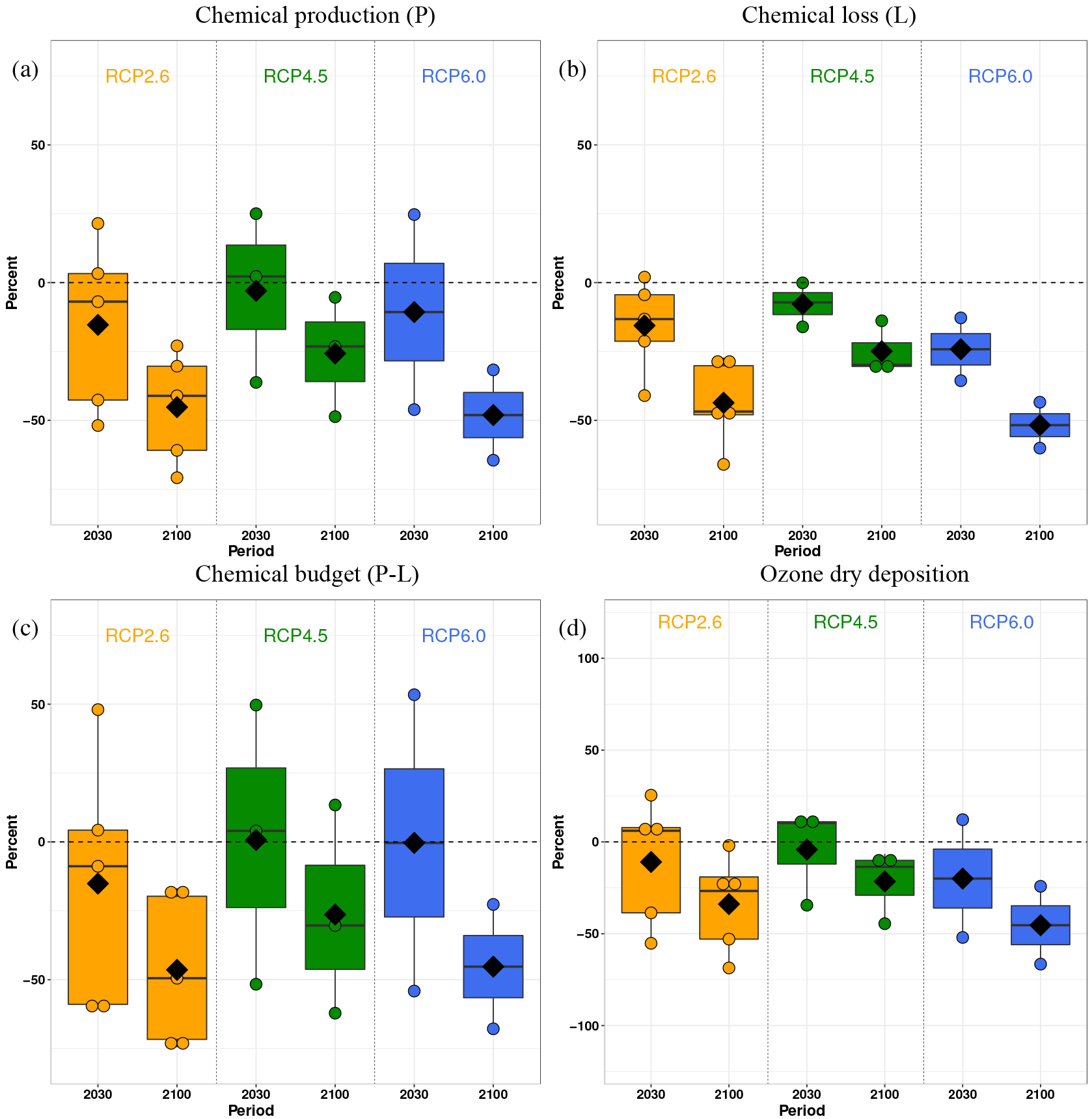
Figure 11Future relative change in surface ozone budget over the MB domain, (a) chemical production (P), (b) chemical loss (L) and (c) chemical budget (P-L) of surface ozone and (d) dry deposition of ozone (D) calculated over the Mediterranean Basin for the JJA period and for RCP2.6 (yellow), RCP4.5 (green) and RCP6.0 (blue). The medians are indicated by the thick horizontal black lines, the multimodel means by filled diamonds, the (25–75 %) range by the colored boxes and minimum/maximum excluding outliers by the whiskers. Each colored point represents a single model. The dashed horizontal line represents the mean for the REF period (2000) and is considered as a reference.
Figure 11 shows the relative changes in summer surface ozone budget terms (P, L, P-L and D) over the MB for RCP2.6, RCP4.5 and RCP6.0. In terms of the chemical ozone budget evolution, we observe that all the terms (P, L and P-L) decrease for RCP2.6 by 2030 and 2100 compared to REF. The percentage decrease is similar for P and L by 2100 and gives a similar decrease of −40 % for the P-L term. For RCP4.5 and RCP6.0, all the terms decrease by 2100 after a slight increase in P-L by 2030 for RCP4.5. We note that all models are in agreement in terms of trends between 2030 and 2100 for these three scenarios.
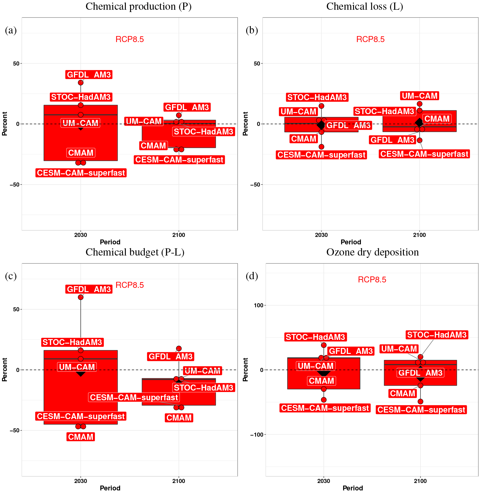
Figure 12Future relative change in surface ozone budget over the MB domain, (a) chemical production (P), (b) chemical loss (L) and (c) chemical budget (P-L) of surface ozone, (d) dry deposition of ozone (D) calculated over the Mediterranean Basin for JJA period and for RCP8.5. The median is indicated by the thick horizontal black line, the multimodel mean by a filled diamond, the (25–75 %) range by the colored box and minimum/maximum excluding outliers by the whisker. Each point represents a single model. The dashed horizontal line represents the mean for the REF period (2000) and is considered as a reference. The future relative change was calculated over the periods 2027–2040 and 2085–2110 (see Table 3).
For RCP8.5 scenario (Fig. 12), the averages of P, L and P-L increase by 2030. For the 2030 to 2100 time slices, the mean relative changes of P, L and P-L are −5, 2 and −10 %, respectively. Nevertheless, the models are not in agreement in terms of the chemical ozone budget evolution for RCP8.5. The terms (P, L and P-L) decrease for GFDL AM3, STOC-HadAM3 and UM-CAM and increase for CMAM and CESM-CAM-superfast. It is difficult to interpret this difference given the complexity of the models. Lacressonnière et al. (2014) have shown that the term P-L decreases over Europe in the short-term period (2030 and 2050) using the MOCAGE chemical transport model for RCP8.5, and Young et al. (2013) have also shown that the net chemical production (P-L) of the global tropospheric ozone decreases between the REF period and 2100 for RCP8.5. Also note that each scenario is represented by a different set of models, except for RCP2.6 and RCP8.5, which are represented by the same set of models, making them comparable in terms of future ozone budget trend. The net influx of ozone is not investigated due to its large uncertainty within a MB box and the limited amount of ACCMIP data (Young et al., 2013). For all scenarios from 2030 to 2100, dry deposition of ozone decreases like surface ozone concentration with a more pronounced decrease for RCP2.6 and RCP6.0 than for RCP4.5. Moreover, the surface ozone budget terms (P, L, P-L and D) decrease by 2100 over the MB for RCP2.6, RCP4.5 and RCP6.0, with a general agreement between models. For RCP8.5, the surface ozone budget terms of each model evolve differently, which explains the non-significant changes in surface ozone and its stagnation over the MB.
The future evolution in surface ozone is investigated in summertime (June, July and August) over the MB, from 2000 to 2100, using the ACCMIP outputs from 13 models. This study was carried out over the MB, considering time slices around 2000, 2030 and 2100, and using the four RCPs. We started by assessing the models used by comparing surface ozone between contemporary era ACCMIP simulations (1990–2010) and gridded observations from the EMEP, WMO-GAW and AirBase network over the MB. Firstly, our approach consists of studying the meteorological parameters (temperature, specific humidity, precipitation) and ozone precursors (CH4 concentration, NOx, VOCs, CO emissions). Secondly, we analyzed the changes in surface ozone and available terms of its budget (chemical budget and dry deposition).
The evaluation of the models against observations over a REF period (2000 time slice) allowed us to understand their behavior in simulating surface ozone. The annual cycle is very well captured by most of the models and the ACCMIP mean shows better performances than most of the models, with a correlation coefficient R=0.93. However, we found that most models overestimate the summer surface observations with ozone being better represented in southern Europe than in the Mediterranean Sea. The model performances do not change between the global and the regional MB scales.
The analysis of meteorological parameters indicates that the temperature increases during the 21st century for all RCPs, according to the RF, by an average of 1.4–6.0 K in 2100 compared to 2000. The specific humidity increases also as a response to the rise of the temperature; precipitation decreases for scenarios that have high RF (RCP6.0 and RCP8.5). Changes in ozone precursors show that CO and NOx decrease constantly, reflecting the emission reduction policy. Changes in ozone concentrations due to VOCs emissions changes are not conclusive given the very large inter-model variability in biogenic VOCs emissions. CH4 increases for RCP8.5 but decreases for other scenarios. RCP8.5 shows a statistically non-significant change in summer surface ozone of −1.3 % (−0.8 %) in 2030 (2100) over the MB, unlike the other RCPs, which show a statistically significant ozone decrease (using the Student t test with 95 % confidence level) of −14 % (−38 %) for RCP2.6, −9 % (−24 %) for RCP4.5 and −10 % (−29 %) for RCP6.0. The net chemical budget (chemical production minus loss) of ozone decreases intensively (25–45 %) from 2000 to 2100 for RCP2.6, RCP4.5 and RCP6.0 and less strongly (−10 %) for RCP8.5. Dry deposition of ozone decreases for all RCPs following surface ozone concentration decreases, especially for RCP2.6 and RCP6.0 that show a large ozone decrease.
The net decrease in surface ozone (between 2000 and 2100) over the MB for RCP2.6 (−38 %), RCP4.5 (−24 %) and RCP6.0 (−29 %) is mainly due to the reduction in ozone precursor emissions. This reduction is relatively the same for RCP2.6 and RCP6.0, despite the marked difference in the global RF of 3.4 W m−2 between the two scenarios, which is mainly dominated by the forcing from CO2. The largest decrease in surface ozone is calculated over the Mediterranean Sea and the eastern part of the Atlantic Ocean, likely due to the increase of specific humidity in these areas. Other dynamical factors can affect the surface ozone evolution over the MB (e.g., increasing stratosphere–troposphere exchange, the recovery of stratospheric ozone, long-range transport).
The surface ozone decrease over the MB for the scenarios RCP2.6, RCP4.5 and RCP6.0 is much more pronounced than the relative changes of the global tropospheric ozone burden. This reflects the fact that the surface ozone over the MB is more controlled by reductions of its precursor emissions, water vapor represented by the increase in the specific humidity and the NOx-limited regime over the MB. In this region, for the RCP8.5 scenario, we showed how the future climate change and in particular the increase in methane concentrations can offset the benefits from the reduction in emissions of ozone precursors.
The model data outputs from the Atmospheric Chemistry and Climate Model Intercomparison Project (ACCMIP) are publicly accessible from the NCAS British Atmospheric Data Centre: http://catalogue.ceda.ac.uk/uuid/ded523bf23d59910e5d73f1703a2d540 (Atmospheric Chemistry and Climate Model Intercomparison Project, 2011).
The gridded global surface ozone metrics data (1971–2015) for atmospheric chemistry model evaluation are publicly available from the Centre for Environmental Data Analysis: https://doi.org/10.5285/897a3958-5bfc-4311-9bb0-01134bf6aefa (Evans and Sofen, 2016).
The authors declare that they have no conflict of interest.
This article is part of the special issue “CHemistry and AeRosols Mediterranean EXperiments (ChArMEx) (ACP/AMT inter-journal SI)”. It is no associated with a conference.
This work is funded in France by the Centre National de Recherches
Météorologiques (CNRM) of Météo-France, the region Occitanie and the
Centre National de Recherches Scientifiques (CNRS). The authors thank all
stakeholders who contributed to the ACCMIP data production and collection. We
thank the two anonymous reviewers for their valuable comments, and we also
express our thanks to Jean-Francois Lamarque and Béatrice Josse for their
valuable comments that greatly improved our
manuscript.
Edited by: William Lahoz
Reviewed by: three anonymous referees
Akritidis, D., Zanis, P., Pytharoulis, I., and Karacostas, T.: Near-surface ozone trends over Europe in RegCM3/CAMx simulations for the time period 1996–2006, Atmos. Environ., 97, 6–18, https://doi.org/10.1016/j.atmosenv.2014.08.002, 2014. a
Atmospheric Chemistry and Climate Model Intercomparison Project: National Centre for Atmospheric Research, Shindell, D., Zeng, G., Lamarque, J. F., Szopa, S., Nagashima, T., Naik, V., Eyring, V., and Collins, W.: The model data outputs from the Atmospheric Chemistry & Climate Model Intercomparison Project (ACCMIP), NCAS British Atmospheric Data Centre, available at: http://catalogue.ceda.ac.uk/uuid/ded523bf23d59910e5d73f1703a2d540 (last access: 22 June 2018), 2011. a
Beekmann, M. and Vautard, R.: A modelling study of photochemical regimes over Europe: robustness and variability, Atmos. Chem. Phys., 10, 10067–10084, https://doi.org/10.5194/acp-10-10067-2010, 2010. a, b
Bell, M. L., McDermott, A., Zeger, S. L., Samet, J. M., and Dominici, F.: Ozone and short-term mortality in 95 US urban communities, 1987–2000, Jama, 292, 2372–2378, https://doi.org/10.1001/jama.292.19.2372, 2004. a
Benjamini, Y. and Hochberg, Y.: Controlling the false discovery rate: a practical and powerful approach to multiple testing, J. R. Stat. Soc. B Met., 57, 289–300, 1995. a
Brook, R. D., Brook, J. R., Urch, B., Vincent, R., Rajagopalan, S., and Silverman, F.: Inhalation of fine particulate air pollution and ozone causes acute arterial vasoconstriction in healthy adults, Circulation, 105, 1534–1536, https://doi.org/10.1161/01.CIR.0000013838.94747.64, 2002. a
Butchart, N. and Scaife, A. A.: Removal of chlorofluorocarbons by increased mass exchange between the stratosphere and troposphere in a changing climate, Nature, 410, 799–802, https://doi.org/10.1038/35071047, 2001. a
Butchart, N., Scaife, A., Bourqui, M., De Grandpré, J., Hare, S., Kettleborough, J., Langematz, U., Manzini, E., Sassi, F., Shibata, K., Shindell, D., and Sigmond, M.: Simulations of anthropogenic change in the strength of the Brewer–Dobson circulation, Clim. Dynam., 27, 727–741, https://doi.org/10.1007/s00382-006-0162-4, 2006. a
Butler, T. M., Stock, Z. S., Russo, M. R., Denier van der Gon, H. A. C., and Lawrence, M. G.: Megacity ozone air quality under four alternative future scenarios, Atmos. Chem. Phys., 12, 4413–4428, https://doi.org/10.5194/acp-12-4413-2012, 2012. a
Cionni, I., Eyring, V., Lamarque, J. F., Randel, W. J., Stevenson, D. S., Wu, F., Bodeker, G. E., Shepherd, T. G., Shindell, D. T., and Waugh, D. W.: Ozone database in support of CMIP5 simulations: results and corresponding radiative forcing, Atmos. Chem. Phys., 11, 11267–11292, https://doi.org/10.5194/acp-11-11267-2011, 2011. a
Coleman, L., Varghese, S., Tripathi, O., Jennings, S., and O'Dowd, C.: Regional-scale ozone deposition to North-East Atlantic waters, Adv. Meteorol., 2010, 243701, https://doi.org/10.1155/2010/243701, 2010. a
Colette, A., Granier, C., Hodnebrog, Ø., Jakobs, H., Maurizi, A., Nyiri, A., Rao, S., Amann, M., Bessagnet, B., D'Angiola, A., Gauss, M., Heyes, C., Klimont, Z., Meleux, F., Memmesheimer, M., Mieville, A., Rouïl, L., Russo, F., Schucht, S., Simpson, D., Stordal, F., Tampieri, F., and Vrac, M.: Future air quality in Europe: a multi-model assessment of projected exposure to ozone, Atmos. Chem. Phys., 12, 10613–10630, https://doi.org/10.5194/acp-12-10613-2012, 2012. a
Collins, W., Derwent, R., Garnier, B., Johnson, C., Sanderson, M., and Stevenson, D.: Effect of stratosphere-troposphere exchange on the future tropospheric ozone trend, J. Geophys. Res.-Atmos., 108, 8528, https://doi.org/10.1029/2002jd002617, 2003. a, b
Danielsen, E. F.: Stratospheric-tropospheric exchange based on radioactivity, ozone and potential vorticity, J. Atmos. Sci., 25, 502–518, https://doi.org/10.1175/1520-0469(1968)025<0502:stebor>2.0.co;2, 1968. a
Derwent, R., Jenkin, M., Saunders, S., Pilling, M., Simmonds, P., Passant, N., Dollard, G., Dumitrean, P., and Kent, A.: Photochemical ozone formation in north west Europe and its control, Atmos. Environ., 37, 1983–1991, https://doi.org/10.1016/s1352-2310(03)00031-1, 2003. a
Doherty, R., Wild, O., Shindell, D., Zeng, G., MacKenzie, I., Collins, W., Fiore, A. M., Stevenson, D., Dentener, F., Schultz, M., Hess, P., Derwent, R. G., and Keating, T. J.: Impacts of climate change on surface ozone and intercontinental ozone pollution: A multi-model study, J. Geophys. Res.-Atmos., 118, 3744–3763, https://doi.org/10.1002/jgrd.50266, 2013. a
Evans, M. J. and Sofen, E. D.: Gridded Global Surface Ozone Metrics data (1971–2015) for Atmospheric Chemistry Model Evaluation –version 2.7, Centre for Environmental Data Analysis, 2 February 2016, https://doi.org/10.5285/897a3958-5bfc-4311-9bb0-01134bf6aefa, 2016. a
Finzi, G., Silibello, C., and Volta, M.: Evaluation of urban pollution abatement strategies by a photochemical dispersion model, Int. J. Environ. Pollut., 14, 616–624, https://doi.org/10.1504/ijep.2000.000586, 2000. a
Fiore, A. M., West, J. J., Horowitz, L. W., Naik, V., and Schwarzkopf, M. D.: Characterizing the tropospheric ozone response to methane emission controls and the benefits to climate and air quality, J. Geophys. Res.-Atmos., 113, D08307, https://doi.org/10.1029/2007jd009162, 2008. a
Fiore, A. M., Dentener, F., Wild, O., Cuvelier, C., Schultz, M., Hess, P., Textor, C., Schulz, M., Doherty, R., Horowitz, L., MacKenzie, I. A., Sanderson, M. G., Shindell, D. T., Stevenson, D. S., Szopa, S., Van Dingenen, R., Zeng, G., Atherton, C., Bergmann, D., Bey, I. Carmichael, G., Collins, W. J., Duncan, B. N., Faluvegi, G., Folberth, G., Gauss, M., Gong, S., Hauglustaine, D., Holloway, T. Isaksen, I. S. A., Jacob, D. J., Jonson, J. E., Kaminski, J. W. Keating, T. J., Lupu, A., Marmer, E., Montanaro, V., Park, R. J., Pitari, G., Pringle, K. J., Pyle, A., Schroeder, S., Vivanco, M. G., Wind, P., Wojcik, G., Wu, S., and Zuber, A.: Multimodel estimates of intercontinental source-receptor relationships for ozone pollution, J. Geophys. Res.-Atmos., 114, D04301, https://doi.org/10.1029/2008jd010816, 2009. a
Forkel, R. and Knoche, R.: Nested regional climate–chemistry simulations for central Europe, C. R. Geosci., 339, 734–746, https://doi.org/10.1016/j.crte.2007.09.018, 2007. a
Fuhrer, J. and Booker, F.: Ecological issues related to ozone: agricultural issues, Environ. Int., 29, 141–154, https://doi.org/10.1016/s0160-4120(02)00157-5, 2003. a
Fujino, J., Nair, R., Kainuma, M., Masui, T., and Matsuoka, Y.: Multi-gas mitigation analysis on stabilization scenarios using AIM global model, Energ. J., 27, 343–353, https://doi.org/10.5547/issn0195-6574-ej-volsi2006-nosi3-17, 2006. a
Ganzeveld, L., Helmig, D., Fairall, C., Hare, J., and Pozzer, A.: Atmosphere-ocean ozone exchange: A global modeling study of biogeochemical, atmospheric, and waterside turbulence dependencies, Global Biogeochem. Cy., 23, GB4021, https://doi.org/10.1029/2008gb003301, 2009. a
Gerasopoulos, E., Kouvarakis, G., Vrekoussis, M., Kanakidou, M., and Mihalopoulos, N.: Ozone variability in the marine boundary layer of the eastern Mediterranean based on 7-year observations, J. Geophys. Res.-Atmos., 110, D15309, https://doi.org/10.1029/2005JD005991, 2005. a
Giorgi, F.: Climate change hot-spots, Geophys. Res. Lett., 33, L08707, https://doi.org/10.1029/2006gl025734, 2006. a
Goldberg, D. L., Vinciguerra, T. P., Anderson, D. C., Hembeck, L., Canty, T. P., Ehrman, S. H., Martins, D. K., Stauffer, R. M., Thompson, A. M., Salawitch, R. J., and Dickerson, R.: CAMx ozone source attribution in the eastern United States using guidance from observations during DISCOVER-AQ Maryland, Geophys. Res. Lett., 43, 2249–2258, https://doi.org/10.1002/2015gl067332, 2016. a
Hedegaard, G. B., Brandt, J., Christensen, J. H., Frohn, L. M., Geels, C., Hansen, K. M., and Stendel, M.: Impacts of climate change on air pollution levels in the Northern Hemisphere with special focus on Europe and the Arctic, Atmos. Chem. Phys., 8, 3337–3367, https://doi.org/10.5194/acp-8-3337-2008, 2008. a
Hedegaard, G. B., Christensen, J. H., and Brandt, J.: The relative importance of impacts from climate change vs. emissions change on air pollution levels in the 21st century, Atmos. Chem. Phys., 13, 3569–3585, https://doi.org/10.5194/acp-13-3569-2013, 2013. a
Hijioka, Y., matsuoka, Y., nishimoto, H., Masui, T., and Kainuma, M.: Global GHG emission scenarios under GHG concentration stabilization targets, Journal of Global Environment Engineering, 13, 97–108, 2008. a
Hu, L., Jacob, D. J., Liu, X., Zhang, Y., Zhang, L., Kim, P. S., Sulprizio, M. P., and Yantosca, R. M.: Global budget of tropospheric ozone: evaluating recent model advances with satellite (OMI), aircraft (IAGOS), and ozonesonde observations, Atmos. Environ., 167, 323–334, https://doi.org/10.1016/j.atmosenv.2017.08.036, 2017. a
Iglesias-Suarez, F., Young, P. J., and Wild, O.: Stratospheric ozone change and related climate impacts over 1850–2100 as modelled by the ACCMIP ensemble, Atmos. Chem. Phys., 16, 343–363, https://doi.org/10.5194/acp-16-343-2016, 2016. a
Im, U., Markakis, K., Poupkou, A., Melas, D., Unal, A., Gerasopoulos, E., Daskalakis, N., Kindap, T., and Kanakidou, M.: The impact of temperature changes on summer time ozone and its precursors in the Eastern Mediterranean, Atmos. Chem. Phys., 11, 3847–3864, https://doi.org/10.5194/acp-11-3847-2011, 2011. a
Jacob, D. J.: Heterogeneous chemistry and tropospheric ozone, Atmos. Environ., 34, 2131–2159, https://doi.org/10.1016/s1352-2310(99)00462-8, 2000. a
Jacob, D. J. and Winner, D. A.: Effect of climate change on air quality, Atmos. Environ., 43, 51–63, https://doi.org/10.1016/j.atmosenv.2008.09.051, 2009. a, b, c, d
Katragkou, E., Zanis, P., Kioutsioukis, I., Tegoulias, I., Melas, D., Krüger, B., and Coppola, E.: Future climate change impacts on summer surface ozone from regional climate-air quality simulations over Europe, J. Geophys. Res.-Atmos., 116, D22307, https://doi.org/10.1029/2011jd015899, 2011. a
Kawase, H., Nagashima, T., Sudo, K., and Nozawa, T.: Future changes in tropospheric ozone under Representative Concentration Pathways (RCPs), Geophys. Res. Lett., 38, L05801, https://doi.org/10.1029/2010gl046402, 2011. a, b
Lacressonnière, G., Peuch, V.-H., Arteta, J., Josse, B., Joly, M., Marécal, V., Saint Martin, D., Déqué, M., and Watson, L.: How realistic are air quality hindcasts driven by forcings from climate model simulations?, Geosci. Model Dev., 5, 1565–1587, https://doi.org/10.5194/gmd-5-1565-2012, 2012. a
Lacressonnière, G., Peuch, V.-H., Vautard, R., Arteta, J., Déqué, M., Joly, M., Josse, B., Marécal, V., and Saint-Martin, D.: European air quality in the 2030s and 2050s: Impacts of global and regional emission trends and of climate change, Atmos. Environ., 92, 348–358, https://doi.org/10.1016/j.atmosenv.2014.04.033, 2014. a, b, c
Lamarque, J.-F., Bond, T. C., Eyring, V., Granier, C., Heil, A., Klimont, Z., Lee, D., Liousse, C., Mieville, A., Owen, B., Schultz, M. G., Shindell, D., Smith, S. J., Stehfest, E., Van Aardenne, J., Cooper, O. R., Kainuma, M., Mahowald, N., McConnell, J. R., Naik, V., Riahi, K., and van Vuuren, D. P.: Historical (1850–2000) gridded anthropogenic and biomass burning emissions of reactive gases and aerosols: methodology and application, Atmos. Chem. Phys., 10, 7017–7039, https://doi.org/10.5194/acp-10-7017-2010, 2010. a, b
Lamarque, J.-F., Shindell, D. T., Josse, B., Young, P. J., Cionni, I., Eyring, V., Bergmann, D., Cameron-Smith, P., Collins, W. J., Doherty, R., Dalsoren, S., Faluvegi, G., Folberth, G., Ghan, S. J., Horowitz, L. W., Lee, Y. H., MacKenzie, I. A., Nagashima, T., Naik, V., Plummer, D., Righi, M., Rumbold, S. T., Schulz, M., Skeie, R. B., Stevenson, D. S., Strode, S., Sudo, K., Szopa, S., Voulgarakis, A., and Zeng, G.: The Atmospheric Chemistry and Climate Model Intercomparison Project (ACCMIP): overview and description of models, simulations and climate diagnostics, Geosci. Model Dev., 6, 179–206, https://doi.org/10.5194/gmd-6-179-2013, 2013. a, b, c, d, e
Langner, J., Engardt, M., Baklanov, A., Christensen, J. H., Gauss, M., Geels, C., Hedegaard, G. B., Nuterman, R., Simpson, D., Soares, J., Sofiev, M., Wind, P., and Zakey, A.: A multi-model study of impacts of climate change on surface ozone in Europe, Atmos. Chem. Phys., 12, 10423–10440, https://doi.org/10.5194/acp-12-10423-2012, 2012. a, b
Lei, H., Wuebbles, D. J., and Liang, X.-Z.: Projected risk of high ozone episodes in 2050, Atmos. Environ., 59, 567–577, https://doi.org/10.1016/j.atmosenv.2012.05.051, 2012. a
Lelieveld, J. and Dentener, F. J.: What controls tropospheric ozone?, J. Geophys. Res.-Atmos., 105, 3531–3551, https://doi.org/10.1029/1999jd901011, 2000. a
Lelieveld, J., Berresheim, H., Borrmann, S., Crutzen, P., Dentener, F., Fischer, H., Feichter, J., Flatau, P., Heland, J., Holzinger, R., Korrmann, R., Lawrence, M. G., Levin, Z., Markowicz, K. M., Mihalopoulos, N., Minikin, A., Ramanathan, V., de Reus, M., Roelofs, G. J., Scheeren, H. A., Sciare, J., Schlager, H., Schultz, M., Siegmund, P., Steil, B., Stephanou, E. G., Stier, P., Traub, M., Warneke, C., Williams, J., and Zierei, H.: Global air pollution crossroads over the Mediterranean, Science, 298, 794–799, https://doi.org/10.1126/science.1075457, 2002. a
Lin, J.-T., Youn, D., Liang, X.-Z., and Wuebbles, D. J.: Global model simulation of summertime US ozone diurnal cycle and its sensitivity to PBL mixing, spatial resolution, and emissions, Atmos. Environ., 42, 8470–8483, https://doi.org/10.1016/j.atmosenv.2008.08.012, 2008. a
Lippmann, M.: Health effects of ozone a critical review, Japca, 39, 672–695, https://doi.org/10.1080/08940630.1989.10466554, 1989. a
Martilli, A., Neftel, A., Favaro, G., Kirchner, F., Sillman, S., and Clappier, A.: Simulation of the ozone formation in the northern part of the Po Valley, J. Geophys. Res.-Atmos., 107, 8195, https://doi.org/10.1029/2001jd000534, 2002. a
Meleux, F., Solmon, F., and Giorgi, F.: Increase in summer European ozone amounts due to climate change, Atmos. Environ., 41, 7577–7587, https://doi.org/10.1016/j.atmosenv.2007.05.048, 2007. a, b, c
Millán, M., Salvador, R., Mantilla, E., and Artnano, B.: Meteorology and photochemical air pollution in southern Europe: experimental results from EC research projects, Atmos. Environ., 30, 1909–1924, https://doi.org/10.1016/1352-2310(95)00220-0, 1996. a
Millán, M., Salvador, R., Mantilla, E., and Kallos, G.: Photooxidant dynamics in the Mediterranean basin in summer: results from European research projects, J. Geophys. Res.-Atmos., 102, 8811–8823, https://doi.org/10.1029/96jd03610, 1997. a
Monks, P. S., Archibald, A. T., Colette, A., Cooper, O., Coyle, M., Derwent, R., Fowler, D., Granier, C., Law, K. S., Mills, G. E., Stevenson, D. S., Tarasova, O., Thouret, V., von Schneidemesser, E., Sommariva, R., Wild, O., and Williams, M. L.: Tropospheric ozone and its precursors from the urban to the global scale from air quality to short-lived climate forcer, Atmos. Chem. Phys., 15, 8889–8973, https://doi.org/10.5194/acp-15-8889-2015, 2015. a
Moss, R. H., Edmonds, J. A., Hibbard, K. A., Manning, M. R., Rose, S. K., Van Vuuren, D. P., Carter, T. R., Emori, S., Kainuma, M., Kram, T., Meehl, G. A., Mitchell, J. F. B., Nakicenovic, N., Riahi, K., Smith, S. J., Stouffer, R. J., Thomson, A. M., Weyant, J. P., and Wilbanks, T. J.,: The next generation of scenarios for climate change research and assessment, Nature, 463, 747–756, https://doi.org/10.1038/nature08823, 2010. a, b
Riahi, K., Grübler, A., and Nakicenovic, N.: Scenarios of long-term socio-economic and environmental development under climate stabilization, Technol. Forecast. Soc., 74, 887–935, https://doi.org/10.1016/j.techfore.2006.05.026, 2007. a
Safieddine, S., Boynard, A., Coheur, P.-F., Hurtmans, D., Pfister, G., Quennehen, B., Thomas, J. L., Raut, J.-C., Law, K. S., Klimont, Z., Hadji-Lazaro, J., George, M., and Clerbaux, C.: Summertime tropospheric ozone assessment over the Mediterranean region using the thermal infrared IASI/MetOp sounder and the WRF-Chem model, Atmos. Chem. Phys., 14, 10119–10131, https://doi.org/10.5194/acp-14-10119-2014, 2014. a
Sandermann Jr., H.: Ozone and plant health, Annu. Rev. Phytopathol., 34, 347–366, https://doi.org/10.1146/annurev.phyto.34.1.347, 1996. a
Schicker, I., Radanovics, S., and Seibert, P.: Origin and transport of Mediterranean moisture and air, Atmos. Chem. Phys., 10, 5089–5105, https://doi.org/10.5194/acp-10-5089-2010, 2010. a
Schnell, J. L., Prather, M. J., Josse, B., Naik, V., Horowitz, L. W., Cameron-Smith, P., Bergmann, D., Zeng, G., Plummer, D. A., Sudo, K., Nagashima, T., Shindell, D. T., Faluvegi, G., and Strode, S. A.: Use of North American and European air quality networks to evaluate global chemistry–climate modeling of surface ozone, Atmos. Chem. Phys., 15, 10581–10596, https://doi.org/10.5194/acp-15-10581-2015, 2015. a
Silibello, C., Calori, G., Brusasca, G., Catenacci, G., and Finzi, G.: Application of a photochemical grid model to Milan metropolitan area, Atmos. Environ., 32, 2025–2038, 1998. a
Sillman, S.: The use of NOy, H2O2, and HNO3 as indicators for ozone-NOx-hydrocarbon sensitivity in urban locations, J. Geophys. Res.-Atmos., 100, 14175–14188, https://doi.org/10.1029/94jd02953, 1995. a
Smith, S. J. and Wigley, T.: Multi-gas forcing stabilization with Minicam, Energ. J., 27, 373–391, https://doi.org/10.5547/issn0195-6574-ej-volsi2006-nosi3-19, 2006. a
Sofen, E. D., Bowdalo, D., Evans, M. J., Apadula, F., Bonasoni, P., Cupeiro, M., Ellul, R., Galbally, I. E., Girgzdiene, R., Luppo, S., Mimouni, M., Nahas, A. C., Saliba, M., and Tørseth, K.: Gridded global surface ozone metrics for atmospheric chemistry model evaluation, Earth Syst. Sci. Data, 8, 41–59, https://doi.org/10.5194/essd-8-41-2016, 2016. a, b, c, d, e
Spivakovsky, C., Logan, J., Montzka, S., Balkanski, Y., Foreman-Fowler, M., Jones, D., Horowitz, L., Fusco, A., Brenninkmeijer, C., Prather, M., Wofsy, S. C., and McElroy, M. B.: Three-dimensional climatological distribution of tropospheric OH: Update and evaluation, J. Geophys. Res., 105, 8931–8980, https://doi.org/10.1029/1999jd901006, 2000. a
Sudo, K., Takahashi, M., and Akimoto, H.: Future changes in stratosphere-troposphere exchange and their impacts on future tropospheric ozone simulations, Geophys. Res. Lett., 30, 2256, https://doi.org/10.1029/2003gl018526, 2003. a
Taylor, K. E.: Summarizing multiple aspects of model performance in a single diagram, J. Geophys. Res.-Atmos., 106, 7183–7192, https://doi.org/10.1029/2000jd900719, 2001. a
Travis, K. R., Jacob, D. J., Fisher, J. A., Kim, P. S., Marais, E. A., Zhu, L., Yu, K., Miller, C. C., Yantosca, R. M., Sulprizio, M. P., Thompson, A. M., Wennberg, P. O., Crounse, J. D., St. Clair, J. M., Cohen, R. C., Laughner, J. L., Dibb, J. E., Hall, S. R., Ullmann, K., Wolfe, G. M., Pollack, I. B., Peischl, J., Neuman, J. A., and Zhou, X.: Why do models overestimate surface ozone in the Southeast United States?, Atmos. Chem. Phys., 16, 13561–13577, https://doi.org/10.5194/acp-16-13561-2016, 2016. a, b
Tukey, J. W.: Exploratory data analysis, vol. 2, Reading, Mass., 1977. a
Van Vuuren, D., Eickhout, B., Lucas, P. L., and Den Elzen, M.: Long-term multi-gas scenarios to stabilise radiative forcing–exploring costs and benefits within an integrated assessment framework, Energ. J., 27, 201–233, https://doi.org/10.5547/issn0195-6574-ej-volsi2006-nosi3-10, 2006. a
Van Vuuren, D., Edmonds, J., Kainuma, M., Riahi, K., Thomson, A., Hibbard, K., Hurtt, G., Kram, T., Krey, V., Lamarque, J., Masui, T., Meinshausen, M., Nakicenovic, N., Smith, S. J., and Rose, S. K.: The representative concentration pathways: an overview, Climatic Change, 109, 5–31, https://doi.org/10.1007/s10584-011-0148-z, 2011. a, b, c, d
Van Vuuren, D. P., Den Elzen, M. G., Lucas, P. L., Eickhout, B., Strengers, B. J., Van Ruijven, B., Wonink, S., and van Houdt, R.: Stabilizing greenhouse gas concentrations at low levels: an assessment of reduction strategies and costs, Climatic Change, 81, 119–159, https://doi.org/10.1007/s10584-006-9172-9, 2007. a
Vautard, R., Builtjes, P., Thunis, P., Cuvelier, C., Bedogni, M., Bessagnet, B., Honore, C., Moussiopoulos, N., Pirovano, G., Schaap, M., Sterni, R., Tarrason, L., and Windj, P.,: Evaluation and intercomparison of Ozone and PM10 simulations by several chemistry transport models over four European cities within the CityDelta project, Atmos. Environ., 41, 173–188, https://doi.org/10.1016/j.atmosenv.2006.07.039, 2007. a
West, J. J., Fiore, A. M., Naik, V., Horowitz, L. W., Schwarzkopf, M. D., and Mauzerall, D. L.: Ozone air quality and radiative forcing consequences of changes in ozone precursor emissions, Geophys. Res. Lett., 34, L06806, https://doi.org/10.1029/2006gl029173, 2007. a, b
Wild, O., Fiore, A. M., Shindell, D. T., Doherty, R. M., Collins, W. J., Dentener, F. J., Schultz, M. G., Gong, S., MacKenzie, I. A., Zeng, G., Hess, P., Duncan, B. N., Bergmann, D. J., Szopa, S., Jonson, J. E., Keating, T. J., and Zuber, A.: Modelling future changes in surface ozone: a parameterized approach, Atmos. Chem. Phys., 12, 2037–2054, https://doi.org/10.5194/acp-12-2037-2012, 2012. a, b, c
Wilks, D.: On “field significance” and the false discovery rate, J. Appl. Meteorol. Clim., 45, 1181–1189, 2006. a
Wise, M., Calvin, K., Thomson, A., Clarke, L., Bond-Lamberty, B., Sands, R., Smith, S. J., Janetos, A., and Edmonds, J.: Implications of limiting CO2 concentrations for land use and energy, Science, 324, 1183–1186, https://doi.org/10.1126/science.1168475, 2009. a
Young, P. J., Archibald, A. T., Bowman, K. W., Lamarque, J.-F., Naik, V., Stevenson, D. S., Tilmes, S., Voulgarakis, A., Wild, O., Bergmann, D., Cameron-Smith, P., Cionni, I., Collins, W. J., Dalsøren, S. B., Doherty, R. M., Eyring, V., Faluvegi, G., Horowitz, L. W., Josse, B., Lee, Y. H., MacKenzie, I. A., Nagashima, T., Plummer, D. A., Righi, M., Rumbold, S. T., Skeie, R. B., Shindell, D. T., Strode, S. A., Sudo, K., Szopa, S., and Zeng, G.: Pre-industrial to end 21st century projections of tropospheric ozone from the Atmospheric Chemistry and Climate Model Intercomparison Project (ACCMIP), Atmos. Chem. Phys., 13, 2063–2090, https://doi.org/10.5194/acp-13-2063-2013, 2013. a, b, c, d, e, f, g, h, i, j, k, l
Yu, S., Eder, B., Dennis, R., Chu, S.-H., and Schwartz, S. E.: New unbiased symmetric metrics for evaluation of air quality models, Atmos. Sci. Lett., 7, 26–34, https://doi.org/10.1002/asl.125, 2006. a
Zeng, G., Pyle, J. A., and Young, P. J.: Impact of climate change on tropospheric ozone and its global budgets, Atmos. Chem. Phys., 8, 369–387, https://doi.org/10.5194/acp-8-369-2008, 2008. a
Zeng, G., Morgenstern, O., Braesicke, P., and Pyle, J.: Impact of stratospheric ozone recovery on tropospheric ozone and its budget, Geophys. Res. Lett., 37, L09805, https://doi.org/10.1029/2010gl042812, 2010. a
Zeng, T., Wang, Y., Chance, K., Browell, E. V., Ridley, B. A., and Atlas, E. L.: Widespread persistent near-surface ozone depletion at northern high latitudes in spring, Geophys. Res. Lett., 30, 2298, https://doi.org/10.1029/2003gl018587, 2003. a