the Creative Commons Attribution 4.0 License.
the Creative Commons Attribution 4.0 License.
 | 03 Jul 2018
In situ observation of atmospheric oxygen and carbon dioxide in the North Pacific using a cargo ship
Yu Hoshina
Yasunori Tohjima
Keiichi Katsumata
Toshinobu Machida
Shin-ichiro Nakaoka
Atmospheric oxygen (O2) and carbon dioxide (CO2) variations in the North Pacific were measured aboard a cargo ship, the New Century 2 (NC2), while it cruised between Japan and the United States between December 2015 and November 2016. A fuel cell analyzer and a nondispersive infrared analyzer were used for the measurement of O2 and CO2, respectively. To achieve parts-per-million precision for the O2 measurements, we precisely controlled the flow rates of the sample and reference air introduced into the analyzers and the outlet pressure. A relatively low airflow rate (10 cm3 min−1) was adopted to reduce the consumption rate of the reference gases. In the laboratory, the system achieved measurement precisions of 3.8 per meg for δ(O2 ∕ N2), which is commonly used to express atmospheric O2 variation, and 0.1 ppm for the CO2 mole fraction. After the in situ observation started aboard NC2, we found that the ship's motion caused false wavy variations in the O2 signal with an amplitude of more than several tens of ppm and a period of about 20 s. Although we have not resolved the problem at this stage, hourly averaging considerably suppressed the variation associated with ship motion. Comparison between the in situ observation and flask sampling of air samples aboard NC2 showed that the averaged differences (in situ–flask) and the standard deviations (±1σ) are −2.8 ± 9.4 per meg for δ(O2 ∕ N2) and −0.02 ± 0.33 ppm for the CO2 mole fraction. We compared 1 year of in situ data for atmospheric potential oxygen (APO; O2 ) obtained from the broad middle-latitude region (140∘ E–130∘ W, 29∘ N–45∘ N) with previous flask sampling data from the North Pacific. This comparison showed that longitudinal differences in the seasonal amplitude of APO, ranging from 51 to 73 per meg, were smaller than the latitudinal differences.


The balance of CO2 emissions from fossil fuel combustion, land biotic CO2 uptake, and ocean CO2 uptake determines long-term change in the atmospheric CO2 burden. At the same time, fossil fuel combustion consumes atmospheric O2, while the land biotic CO2 uptake is accompanied by the emission of O2 into the atmosphere. Additionally, today's ocean is considered to be a weak source of O2 because of recent ocean warming (Bopp et al., 2002; Keeling and Garcia, 2002; Plattner et al., 2002). The CO2 and O2 exchanges for biotic processes and fossil fuel combustion are stoichiometrically related, and the fossil fuel consumption rate can be reliably estimated from energy statistics. Therefore, coupled measurements of atmospheric CO2 and O2 have been used to constrain global CO2 budgets by simultaneously solving the equations for the atmospheric CO2 and O2 budgets (Keeling and Shertz, 1992; Battle et al., 2000, 2006; Manning and Keeling, 2006; Tohjima et al., 2008; Ishidoya et al., 2012).
Atmospheric O2 measurements are also useful for understanding air–sea gas exchange. This is based on the fact that the air–sea exchange of O2 is more than 1 order of magnitude faster than that of CO2; the chemical equilibrium of dissolved inorganic carbon (dissolved CO2, bicarbonate, and carbonate ions) in seawater suppresses the air–sea exchange of CO2 (e.g., Keeling et al., 1993). For example, seasonality in ocean biotic activity and sea surface temperature is poorly reflected in air–sea CO2 exchange, while oceanic O2 fluxes show clear seasonal variations. The role of atmospheric O2 as a tracer of air–sea gas exchange is emphasized by the introduction of the tracer atmospheric potential oxygen (APO), which is defined as APO = O2 (Stephens et al., 1998), where 1.1 represents the −O2 ∕ CO2 exchange ratio associated with land biotic activity (Severinghaus, 1995). Since APO is invariant with respect to land biotic O2 and CO2 exchange and predominantly reflects air–sea gas exchange, spatiotemporal variations in APO have been used to study gas fluxes associated with ocean ventilation (Lueker et al., 2003) and ocean spring bloom (Yamagishi et al., 2008) to estimate net ocean production (Keeling and Shertz, 1992; Balkanski et al., 1999; Nevison et al., 2012) and to validate ocean biogeochemical models (Stephens et al., 1998; Naegler et al., 2007; Nevison et al., 2008, 2015, 2016).
The precision required to detect atmospheric O2 variation is at the µmol mol−1 (ppm) level, which is considerably smaller than the atmospheric O2 mole fraction of about 21 %. Keeling (1988) was the first to develop an atmospheric O2 measurement technique with this precision using an interferometer and showing the usefulness of O2 measurements to study the global carbon cycle. Since then, several O2 measurement techniques based on a mass spectrometer (Bender et al., 1994), a paramagnetic analyzer (Manning et al., 1999), a fuel cell analyzer (Stephens et al., 2007), and a vacuum ultraviolet absorption photometer (Stephens et al., 2003) have been developed and applied to atmospheric observations (cf. Keeling and Manning, 2014). When the change in atmospheric O2 concentration is compared with that of CO2, it is expressed as a deviation of the O2 ∕ N2 ratio from an arbitrary reference according to
where the subscripts sam and ref represent sample and reference gases, respectively, and the δ(O2 ∕ N2) value is usually converted to a “per meg” value, which approximates parts per million, by multiplying it by 106 (Keeling and Shertz, 1992). The mole fraction is not used as a measure of O2 abundance because the changes in the mole fraction of major atmospheric constituents like O2 are sometimes very confusing. For example, adding 1 µmol of O2 to an air parcel containing 1 mol of dry air results in a 0.79 ppm increase in the O2 mole fraction, and adding 1 µmol of CO2 results in not only a 1 ppm increase in the CO2 mole fraction but also a 0.21 ppm decrease in the O2 mole fraction. These confusing results are attributed to influences of the changes in the total number of moles in the air parcel on the mole fractions or a dilution effect (e.g., Keeling et al., 1998; Tohjima, 2000). However, adding 1 µmol of O2 to 1 mol of dry air, which contains 0.2094 mol of O2 (Tohjima et al., 2005), always results in a 4.77 per meg change in the δ(O2 ∕ N2) value.
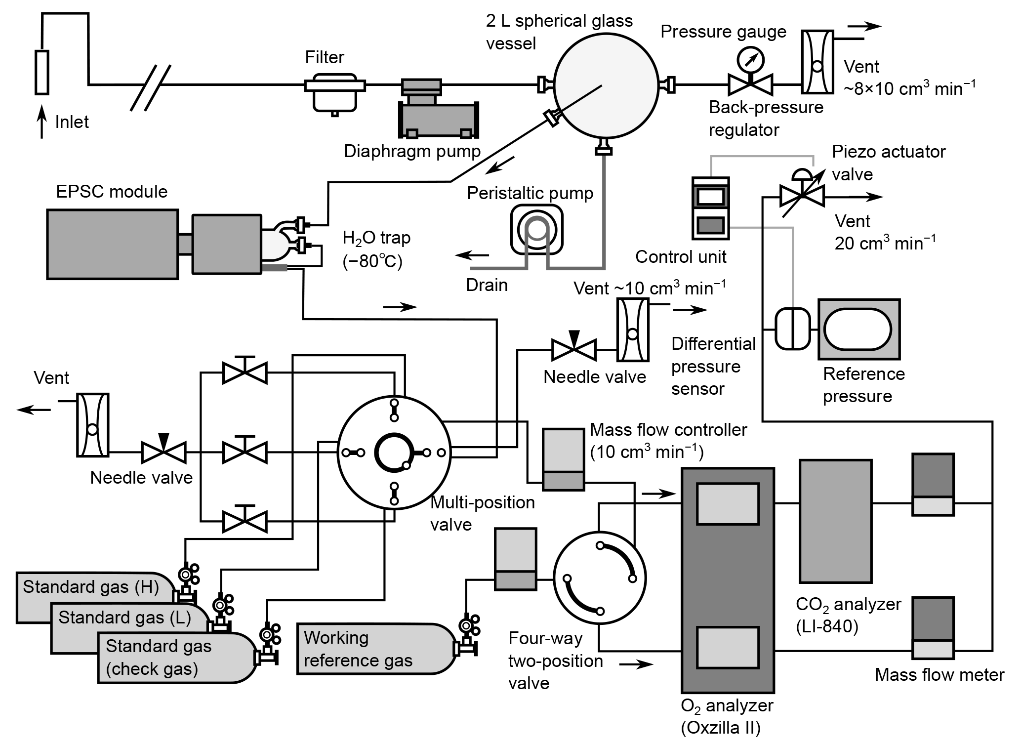
Figure 1Schematic diagram of atmospheric O2 and CO2 measurement system used aboard the cargo ship NC2.
The National Institute of Environmental Studies, Japan (NIES) also developed a technique to measure atmospheric O2 based on a gas chromatograph equipped with a thermal conductivity detector (GC–TCD; Tohjima, 2000). NIES began measuring atmospheric O2 and CO2 by collecting air samples in glass flasks at two monitoring stations, Hateruma Island in July 1997 and Cape Ochiishi in December 1998 (Tohjima et al., 2003, 2008). Additionally, to extend the observation area, we started flask sampling aboard cargo ships sailing between Japan and Australia–New Zealand (Oceanian route) and between Japan and North America (North American route) in December 2011 (Tohjima et al., 2005, 2012). In situ measurements of atmospheric O2 using the GC–TCD technique also started aboard a cargo ship between Japan and Australia–New Zealand in 2007 (Yamagishi et al., 2012).
These O2 and CO2 data from widespread Pacific regions were used to investigate the spatial distribution of the climatological seasonal cycle of APO and the annual mean values of APO (Tohjima et al., 2012). Latitudinal transects of the data in the western Pacific region revealed that variation in the magnitude of the bulge in annual mean APO was associated with the El Niño–Southern Oscillation cycle (Tohjima et al., 2015). This analysis was made possible by the relatively high spatiotemporal sampling density in the western Pacific. In contrast, the spatiotemporally sporadic APO data obtained from the North American route made it difficult to investigate interannual variations in the northern and eastern North Pacific. In 2015, Pickers et al. (2017) started in situ observations of atmospheric O2 and CO2 with a fuel cell analyzer and nondispersive infrared analyzer aboard a commercial container ship regularly traveling in the Atlantic Ocean between Hamburg, Germany and Buenos Aires, Argentina. They also showed the usefulness of continuous observation to reveal the spatiotemporal APO distribution. Therefore, in December 2015, we initiated a program of in situ measurements aboard a cargo ship, the New Century 2 (NC2), sailing between Japan (Tahara port) and North America.
Since June 2014, atmospheric greenhouse gas measurements, including flask sampling (seven flasks per round-trip), have been conducted aboard NC2 along the North American route in the Pacific. We also had an opportunity to install an atmospheric O2 measurement system aboard NC2. However, since the onboard space allotted to us was limited, we had to make the measurement system smaller by reducing the number of cylinders required for the system. In addition, since it is difficult to load and unload high-pressure gas cylinders on ocean-going ships, we needed to reduce the consumption rate of reference gases to reduce the cylinder exchange frequency. With these constraints, the GC–TCD technique, which requires at least 16 m3 of He as a carrier gas for 1 year of continuous O2 observation, was unsuitable for use aboard NC2. Therefore, we developed a low-flow system to perform in situ atmospheric O2 and CO2 measurements aboard NC2. In this paper, we present the details of the measurement system and report its fundamental performance in laboratory testing. We also discuss a problem that occurred when the measurement system was installed aboard NC2. Finally, we present 1 year of atmospheric O2, CO2, and APO data and discuss the longitudinal distribution of the seasonal APO cycle in the North Pacific.
2.1 Analytical system
Figure 1 is a schematic diagram of the in situ observation system used aboard NC2. We used a fuel cell analyzer (Oxzilla II; Sable Systems, USA) and a nondispersive infrared analyzer (LI-840A; LI-COR, USA) for the onboard measurement of O2 and CO2, respectively. After passing through a polypropylene cartridge filter with a mesh size of 7 µm (MCP-7-C10S; ADVANTEC, Japan), the sample air is drawn by a diaphragm pump (MOA-P108-HB; Gast Manufacturing, USA) at a flow rate of about 8×103 cm3 min−1 and introduced into a spherical glass vessel with a volume of about 2×103 cm3. The air is vented to the atmosphere through a back-pressure regulator (6800AL; KOFLOC, Japan), which keeps the pressure inside the spherical vessel at about 0.05 MPa above ambient pressure. Water that condenses within the spherical vessel is drained from the bottom by a peristaltic pump (7016-21; Masterflex, USA). The sample gas for the O2 and CO2 measurements is drawn from the center of the spherical vessel through 1∕16 inch stainless steel (SUS) tubing. The technique of sampling from a spherical glass vessel was adopted to reduce the fractionation of the O2 / N2 ratio (Yamagishi et al., 2008).
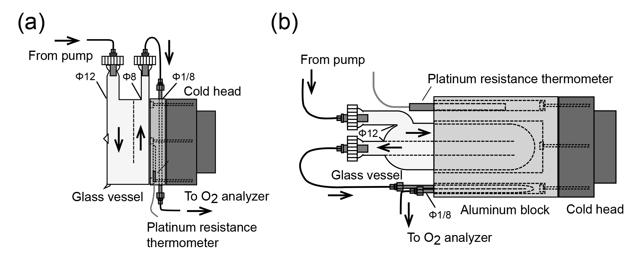
Figure 2Schematic diagram of the (a) first and (b) second versions of the cold trap for reducing water vapor in samples.
The gas sampled from the spherical vessel is introduced into a two-stage cold trap (−80 ∘C) to reduce the water vapor concentration to less than 1 ppm. Details of the cold trap are presented in Sect. 2.2. The dried sample gas and working reference gas, which is supplied from a high-pressure cylinder, are introduced into the two fuel cells of the O2 analyzer via two mass flow controllers (SEC-E40MK3; HORIBA STEC, Japan) and a four-way two-position valve (AC4UWE; Valco Instruments Co. Inc., USA). The mass flow controllers regulate the flow rates of the two gas streams with a precision of 0.01 cm3 min−1. The dried sample air and working reference air alternately pass through each fuel cell at intervals of 2 min by switching the four-way two-position valve. The CO2 analyzer is placed downstream of one of the fuel cells. The flow rates of the outflows from the CO2 analyzer and the other fuel cell are monitored by mass flow meters (SEF-E40; HORIBA STEC, Japan) with a precision of 0.01 cm3 min−1. We adjusted the settings of the mass flow controllers until the readings of the mass flow meters for the two airstreams matched. The outflows of the mass flow meters are combined and vented to the atmosphere via a piezo actuator valve (PV-1202MC; HORIBA STEC, Japan). The outlet pressures of the analyzers are kept at the same absolute value at all times by actively matching them to a reference pressure using the piezo actuator valve and a differential pressure sensor (model 204; Setra Systems, USA).
Before the dried sample gas is introduced into the mass flow controller, it passes through a multi-position valve (EMTCSD6MWM; Valco Instruments Co. Inc., USA) to which three standard gases are connected. During the calibration procedures, the multi-position valve selects the standard gases instead of the sample air, which is vented to the ambient air via a needle valve (2204; KOFLOC, Japan) at a flow rate about 10 cm3 min−1. The 48 L aluminum cylinder for the working reference gas and the three 10 L aluminum cylinders for the standard gases are stored horizontally in thermally insulated boxes.
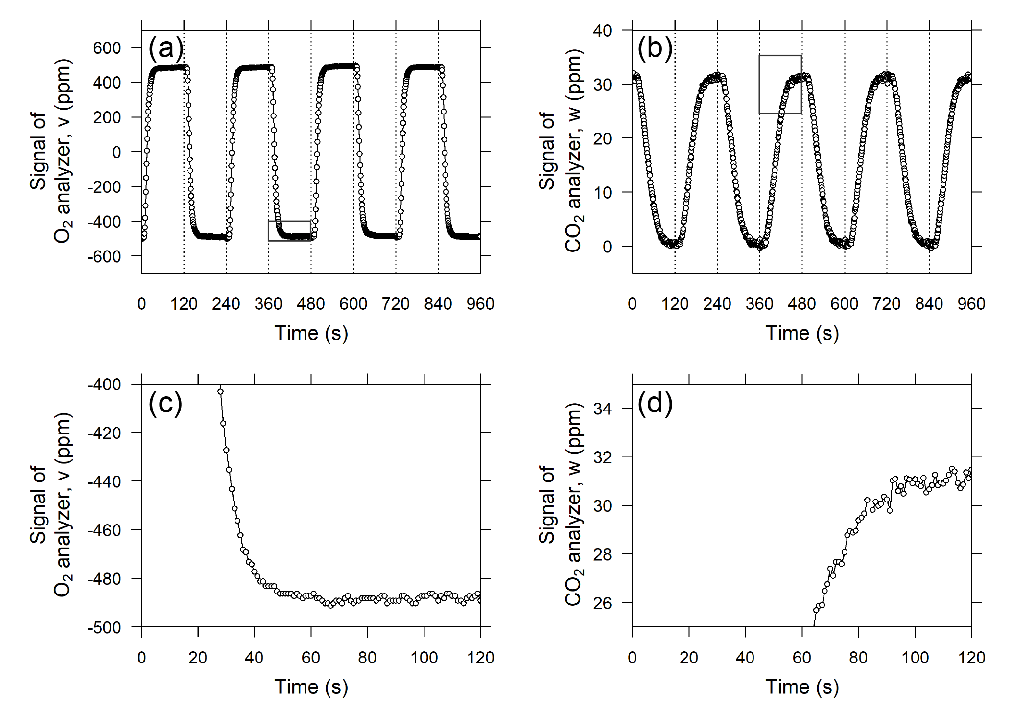
Figure 3Temporal variations in the output signals of the (a) O2 analyzer and (b) CO2 analyzer when standard air from a high-pressure cylinder was measured as sample air. The vertical dashed lines denote the timing of valve switching. Panels (c) and (d) are close-ups of areas marked with rectangles in panels (a) and (b), respectively, and the horizontal axis shows the time from valve switching.
Custom software developed in LabVIEW (National Instruments Co., USA) running on a PC controls valve operation and the acquisition of digital data from the O2 and CO2 analyzers and analog data from the mass flow and pressure sensors.
2.2 Cold trap
Among the constituents of tropospheric air, water vapor shows the widest range of variation, which causes apparent variations in the O2 mole fraction of the air because atmospheric O2 is a major constituent of air (∼ 21 %). For example, a water vapor increase of 1 ppm causes a 0.2 ppm apparent decrease in the O2 mole fraction. Therefore, a two-stage cold trap was adopted to reduce the water vapor in the sample air to less than 1 ppm. Figure 2a shows the first version of the cold trap, which consisted of a free-piston Stirling cooler (FPSC) module (SC-UE15R; Twinbird, Japan), two disk-shaped aluminum blocks, a 1∕8 inch SUS tube, and a drum-shaped glass vessel with a volume of about 1.0×103 cm3. The aluminum blocks had four grooves for the 1∕8 inch SUS tubes, including spare tubes to address clogging. The aluminum blocks were placed between the cold head of the FPSC module and the glass vessel and contact was tight. A platinum resistance thermometer was inserted into the aluminum block, and a temperature controller (E5CC; OMRON, Japan) regulated the FPSC module to maintain the aluminum blocks at −80 ∘C. The sample air was dried by passing through the glass vessel first and then the SUS tube.
When the first cold trap was used for preliminary measurements at NIES during the summer (with high humidity), it worked without clogging for at least 1 month, which is the typical duration for a round-trip using the North American route. However, the measurements were often interrupted because the SUS tube and inlet of the glass vessel clogged when it was used aboard NC2, and the frequency of clogging increased as the season progressed from winter to spring to summer.
Thus, we changed the cold trap to the second design shown in Fig. 2b. In the second version of the cold trap, the cylindrical aluminum block with several holes is in contact with the cold head of the FPSC module, and a cylindrical glass vessel (volume of about 1.5 × 103 cm3) and 1∕8 inch SUS tube are inserted in the holes. The cold head and the aluminum block are insulated by a polyethylene resin cover. We began to use this cold trap for the shipboard measurements in September 2016, and the cold trap has not clogged since that time due to the more complete chilling of the glass vessel.
2.3 Calculation of ΔO2, ΔCO2, and δ(O2 ∕ N2)
The O2 analyzer, equipped with two fuel cell sensors, was designed to precisely measure the difference in the O2 mole fraction between two airstreams. Therefore, the change in the O2 mole fraction of the sample gas is reported as a relative change with respect to the working reference gas, which is supplied from the high-pressure aluminum cylinder (48 L). In previous studies (e.g., Stephens et al., 2007; Thompson et al., 2007; van der Laan-Luijkx et al., 2010; Goto et al., 2013), the sample and reference air are alternately introduced into each fuel cell sensor by switching the four-way two-position valve at 1 to 5 min intervals. In this study, we adopted 2 min for the valve-switching intervals in light of the responses of the O2 and CO2 analyzer after valve switching, as described below. Figure 3a shows the temporal variation in the differential output signal of the O2 analyzer during a test run in which a reference gas from a high-pressure cylinder was used as a sample gas. Although the flow rate in this system (10 cm3 min−1) is more than 4 times slower than the flow rates used in previous studies, the output signal shows an almost rectangular shape. The signal plateaus at least 1 min after the valve switching, and the output signal is averaged from the second minute of the cycle (Fig. 3c). The deviation of the O2 mole fraction in the sample gas from that of the working reference gas for the ith 2 min interval, ΔO2,i, is computed based on the 1 min average according to the following equation:
where vi represents the average of the output signal for the second minute of the ith 2 min interval and the output signal represents the difference of the sample gas minus working reference gas when i is an odd number greater than 1.
In contrast to the O2 analyzer, the CO2 analyzer alternately measures the sample and working reference gases. The temporal variation in the output signal of the CO2 analyzer is depicted in Fig. 3b and d. As shown in the figure, the output signal does not plateau until after more than 90 s because of the relatively low flow rate in comparison with the volume of the optical cell of the LI-840A analyzer (14.5 cm3). Therefore, we compute an average of the output signal for the last 20 s of each 2 min interval. Then, the deviation of the CO2 mole fraction of the sample gas from the working reference gas, ΔCO2,i, is computed according to
where wi represents the average of the last 20 s of data for the ith 2 min interval. Again, the sample gas is introduced into the CO2 analyzer when i is an odd number greater than 1.
The variation in atmospheric O2 is expressed as the change in δ(O2 ∕ N2) with respect to an arbitrary reference value, and δ(O2 ∕ N2) is defined according to Eq. (1). Based on the ΔO2 and ΔCO2 values, δ(O2 ∕ N2) is given by the following equation:
where represents the O2 mole fraction in dry air (.2094; Tohjima et al., 2005). In this calculation, we assume that only O2 and CO2 show more than parts-per-million-level variation among all constituents of dry air, except nitrogen.
The time series of δ(O2 ∕ N2) and ΔCO2 calculated by Eqs. (2), (3), and (4) for “sample” gas provided from a high-pressure cylinder against the working reference air are plotted in Fig. 4. The standard deviations for δ(O2 ∕ N2) and ΔCO2 calculated from 20 h of data are 3.8 per meg and 0.1 ppm, respectively, which likely represents the best possible precision because the measurements were taken in an air-conditioned laboratory.
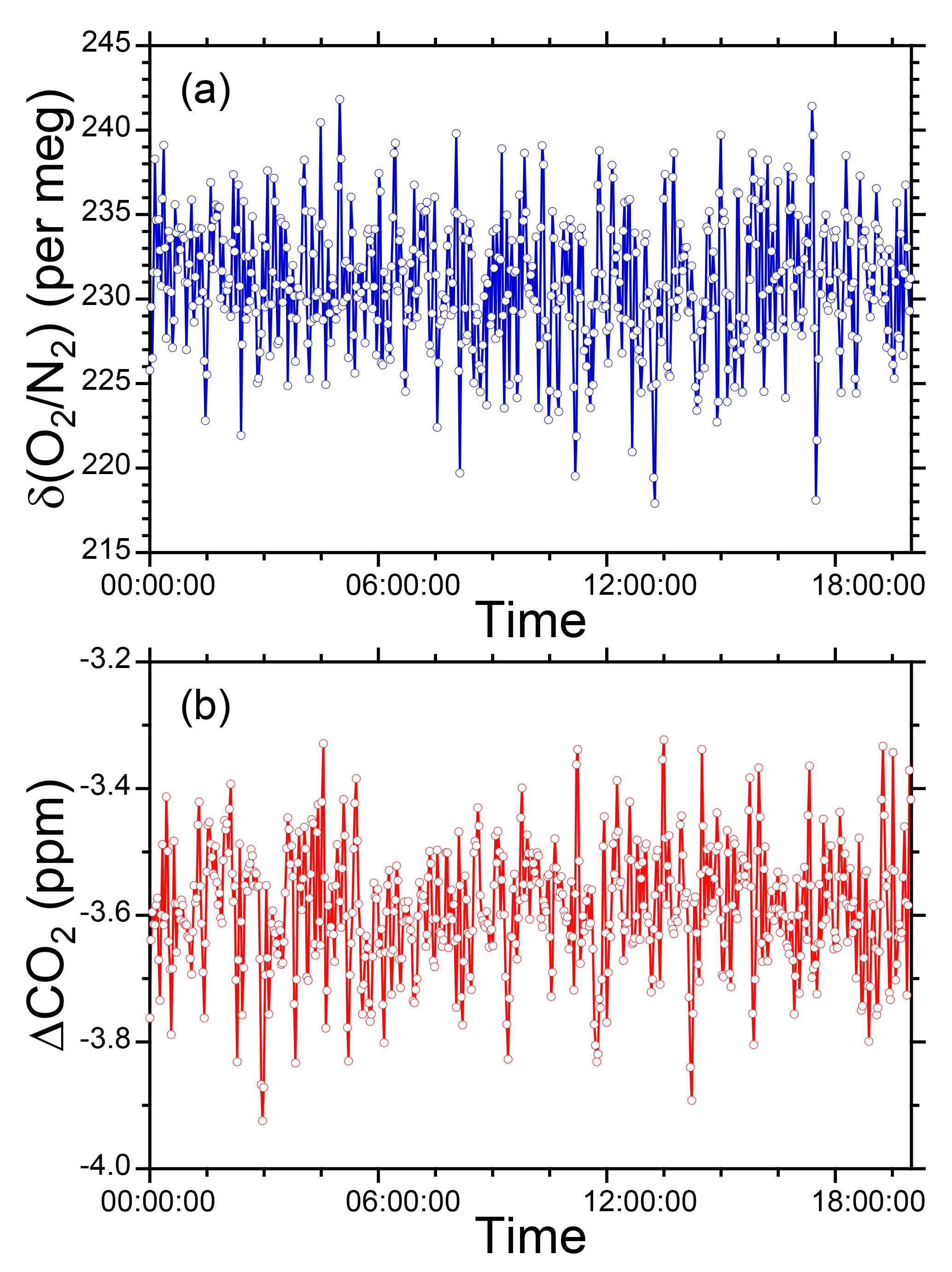
Figure 4Time series of δ(O2 ∕ N2) and ΔCO2 calculated by Eqs. (2), (3), and (4) for sample air provided from a high-pressure cylinder against the working reference.
2.4 Preliminary measurements of atmospheric O2 and CO2
We conducted preliminary observations of atmospheric O2 and CO2 variations at Tsukuba, Japan during the period 10–17 July 2015 to examine the performance of the O2 and CO2 measurement system. Outside air was drawn by the diaphragm pump from an air intake placed on top of our laboratory building. Two standard gases with high (−270 per meg) and low (−579 per meg) δ(O2 ∕ N2) values were repeatedly introduced into the O2 analyzer for 32 min each at intervals of 25 h. We determined a single calibration line of linear response function for δ(O2 ∕ N2) values from all the measurements of the two standard gases during the observation. As for the CO2 mole fraction, a single calibration line of linear function was determined from measurements of three standard gases with 387, 406, and 434 ppm only before the observation. The δ(O2 ∕ N2) value and CO2 mole fraction were reported in our own original scales: the NIES δ(O2 ∕ N2) scale (Tohjima et al., 2008) and the NIES 09 CO2 scale (Machida et al., 2011).
As shown in Fig. 5, the observed δ(O2 ∕ N2) revealed a diurnal cycle with an increase in daytime and decrease at nighttime. This cycle was inversely correlated with the CO2 mole fraction. A scatter plot of CO2 and δ(O2 ∕ N2) shows a clear negative correlation with the ΔO2 ∕ ΔCO2 slope of −1.189 ± 0.004, which is close to the land biotic O2 to CO2 exchange ratio of −1.10 ± 0.05. Since the observation was conducted in summer and coal consumption is limited in Tsukuba, the ΔO2 ∕ ΔCO2 slope means that the observed CO2 changes can be predominantly attributed to activity on land. During the observation, 32 min measurements of a check gas (CPD-00012: −426 per meg for δ(O2 ∕ N2) and 407.12 ppm for CO2) supplied from an aluminum 10 L cylinder were repeated twice daily. The δ(O2 ∕ N2) values and the CO2 mole fractions of the check gas showed steady values (Fig. 5); the average and the standard deviation (±1σ) were −427.5 ± 4.1 per meg for δ(O2 ∕ N2) and 407.11 ± 0.11 ppm for CO2. Moreover, there was no significant drift in the LI-840A analyzer during this observation. These results indicate the stability of the O2 and CO2 measurement system.
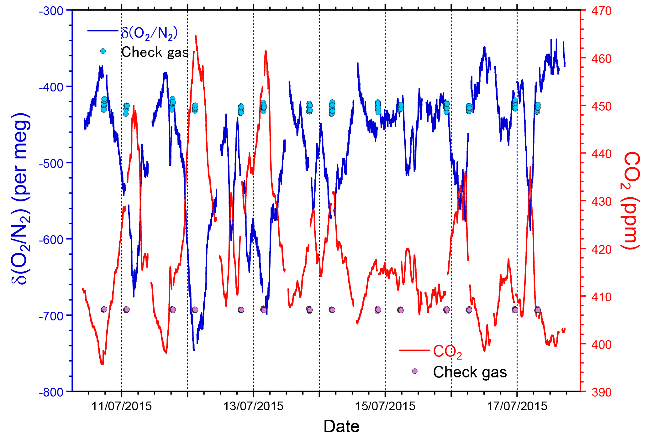
Figure 5Time series of δ(O2 ∕ N2) (blue, left axis) and CO2 mole fraction (red, right axis) observed at Tsukuba during 10–17 July 2015. The δ(O2 ∕ N2) and CO2 mole fraction of the periodically measured check gas are also depicted as light blue and pink circles, respectively.
2.5 In situ measurements aboard NC2
In December 2015, the measurement system was installed in a deckhouse aboard NC2. An air intake was placed on a left-side deck rail of the navigation bridge, and air was drawn via a DK tube (NITTA, Japan) with an outer diameter of 10 mm and a length of about 50 m. A 48 L aluminum cylinder for the working reference gas and three 10 L aluminum cylinders for the O2 and CO2 standard gases were placed in thermally insulated boxes, which were laid horizontally on a shelf to minimize the inhomogeneous distribution of δ(O2 ∕ N2) within the cylinders associated with temperature and pressure gradients (Keeling et al., 1998, 2007).
The two standard gases with −579 per meg (tank CPD-00010) and −270 per meg (tank CPD-00011) were used for calibration of the O2 analyzer. Since the CO2 mole fractions of these two standard gases are almost the same (∼ 407 ppm), we additionally used a third standard gas with a CO2 mole fraction of 448.3 ppm (tank CPB-17350) to calibrate the CO2 analyzer. During every 24 h period, these three standard gases were measured for 32 min each. To determine the calibration lines for both the O2 and CO2 analyzers precisely, measurements of the three standard gases were repeated over 24 h when NC2 berthed at the port of Tahara, Japan.
3.1 Influence of ship motion
After beginning the in situ measurements aboard NC2, we found that the ship motions did not affect the response of the CO2 analyzer but did seriously affect the response of the O2 analyzer. Figure 6a and b show temporal variations in the output signal of the O2 analyzer for the standard gas when NC2 was berthed at the port of Tahara and was cruising on the Pacific Ocean, respectively. The output signal during the cruise (Fig. 6b and d) shows apparent variations with peak-to-peak amplitudes of more than several tens of ppm and peak-to-peak periods of about 20 s. Pickers (2016) reported that similar apparent variations caused by ship motion were superimposed on the output signals of individual fuel cells in an Oxzilla II analyzer. However, in the Pickers instrument, the differential signal of both fuel cells did not show apparent variations because the motion-induced variations were almost compensated for completely by the differential signals.
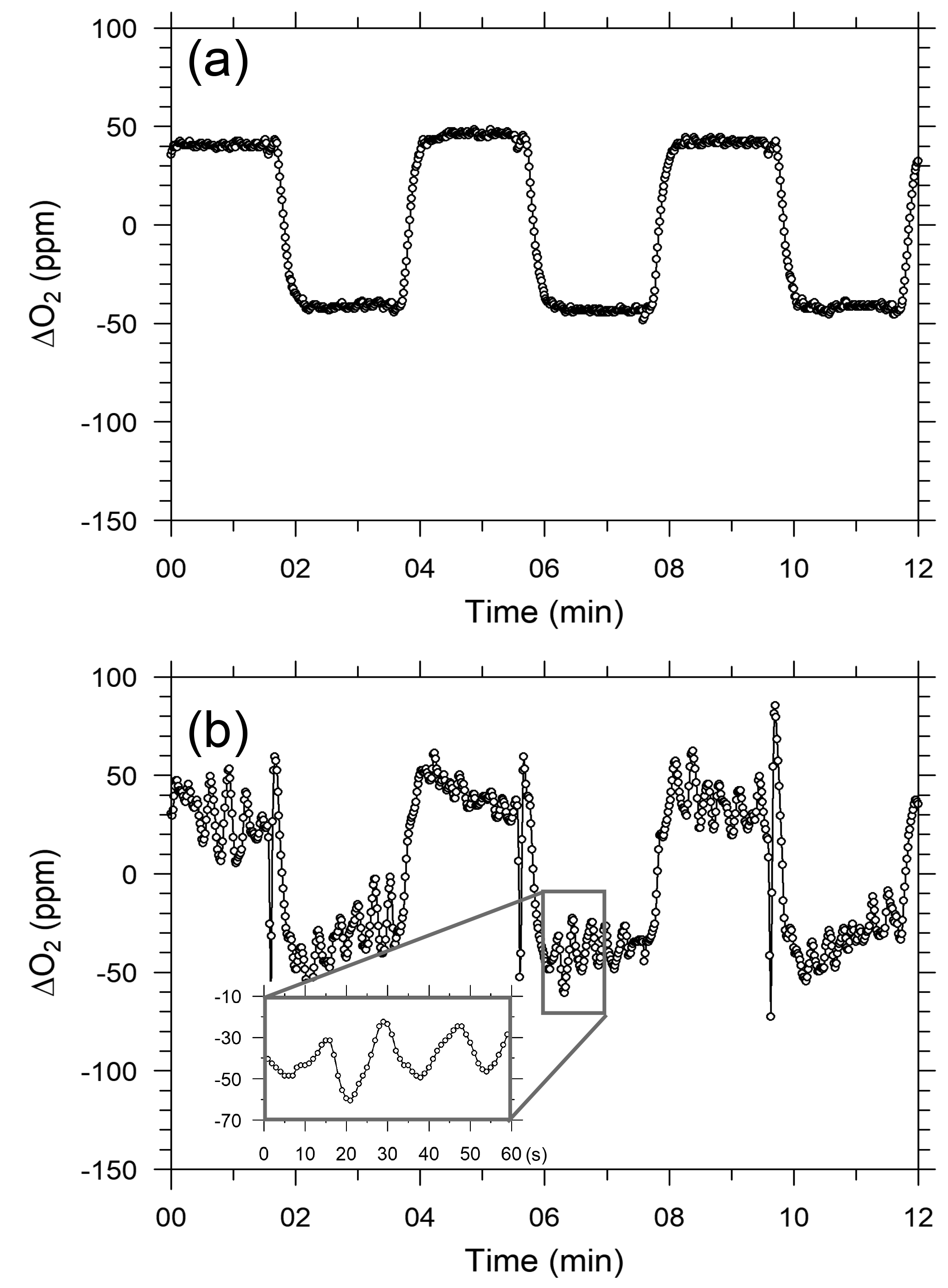
Figure 6Temporal variations in differential output signals of the O2 analyzer for six measurement cycles of O2 standard gas while the ship was (a) in harbor and (b) cruising.
We installed a three-dimensional accelerometer on the O2 analyzer on 3 March 2016 to examine the relationship between the Oxzilla output signals and the ship's motion. The apparent variations in the output signal were associated with the variations in the acceleration of one axis or another and both amplitudes were roughly proportional to each other. However, we have not succeeded in describing the apparent variations with a linear function of the measured accelerations. This is because the sensitivity of the O2 analyzer to the acceleration along the three axes seems to be unstable with time. Therefore, at this stage we cannot remove the apparent variations associated with the ship motions with a simple algorithm.
Figure 7 shows temporal variations in the δ(O2 ∕ N2) value of the two standard gases relative to the working gas during the 1-year period of this study. In the figure, each blue circle represents the 32 min average of the standard gas during the voyages. The standard deviations of the 32 min averages were less than 13 per meg, suggesting that the averaging procedure for several tens of minutes can effectively suppress the errors caused by ship motion. For example, the expected standard deviation of the hourly δ(O2 ∕ N2) value for the standard gases is 9 per meg ().

Figure 7Time series of differences in δ(O2 ∕ N2) for two standard gases, (a) CPD-00011 and (b) CPD-00010, with respect to the working reference gas as determined aboard NC2 during the 1-year period of this study. Blue circles represent 32 min average values of standard gas measurements carried out at 24 h intervals. Black circles represent the averages of calibrations conducted when NC2 was berthed at the port of Tahara, and the error bars represent standard deviations.
The uncertainties in the 32 min averages of the standard gases are too large for calibration of the O2 analyzer. In Fig. 7, the average δ(O2 ∕ N2) values of the standard gases determined when NC2 was berthed at the port of Tahara are also plotted as black circles with error bars showing the standard deviations. Unfortunately, the standard deviations for the standard gases were larger than the expected values obtained in our laboratory, as discussed in Sect. 2.3. However, the standard errors were lower than 2 per meg because the measurements were continued for more than 5 h for the individual standard gases. Therefore, we calibrated the O2 analyzer using calibration lines based on the results at the port just before and after each round-trip voyage.
3.2 Comparison between flask sampling and in situ observations
During the 1-year period from December 2015 through November 2016, the in situ measurements of the atmospheric O2 and CO2 were conducted during nine round-trip voyages, from NC2-123 to NC2-131, along the North American route. The individual cruise tracks are depicted in Fig. 8a, in which thin lines correspond to intervals of missing measurements. We obtained no in situ data during the two westbound voyages of NC2-123 and NC2-128 because the cold trap became clogged. Along with the in situ measurements, air samples were collected in seven 2.5 L glass flasks at fixed longitudes (130, 145, 160, 175∘ W, 170, 155, and 145∘ E) during each westbound cruise.

Figure 8(a) Cruise tracks of NC2 for nine round-trips (NC2-123–NC2-131) during the period from December 2015 to November 2016. Thin lines represent intervals during which in situ measurements aboard NC2 were interrupted. (b) Longitudinal distribution of hourly APO taken from the nine cruises. 5 h running averages are applied to the hourly data to reduce signal noise.
The time series of δ(O2 ∕ N2), CO2, and APO data taken from the in situ measurements and the flask samplings are shown in Fig. 9. The APO is computed based on the δ(O2 ∕ N2) and CO2 mole fraction in accordance with the following equation:
where 1850 is an arbitrary APO reference point adopted by NIES. In Fig. 9, each point for the in situ measurement represents the hourly average, and the data outside the longitudinal range between 140∘ E and 128∘ W are excluded because of significant contamination by anthropogenic emissions from the coastal regions of both Japan and North America. The time series in Fig. 9 clearly shows seasonal cycles and the in situ data seem to agree with the flask data. The differences in the δ(O2 ∕ N2), CO2, and APO values between the in situ and the 39 flask measurements (in situ–flask) are depicted in Fig. 10. The averaged differences with standard deviations were −2.8 ± 9.4 per meg of δ(O2 ∕ N2), −0.02 ± 0.33 ppm of CO2, and −2.9 ± 9.5 per meg of APO. Taking into account the uncertainties in the flask measurements (5 per meg for δ(O2 ∕ N2) and 0.05 ppm for CO2 measurements; Tohjima et al., 2003), we conclude that the uncertainties in the in situ measurements aboard NC2 were 8.0 per meg for δ(O2 ∕ N2) and 0.33 ppm for CO2. The differences between flask sampling and in situ measurements by the GC–TCD method were reported as −0.6 ± 9.1 per meg of APO on the Oceanian route (Tohjima et al., 2015), and 7.0 ± 9.9 per meg of δ(O2 ∕ N2) at Cape Ochiishi (Yamagishi et al., 2008). From these results, we conclude that the reliability of the O2 measurements in this study is similar to that of the GC–TCD method.
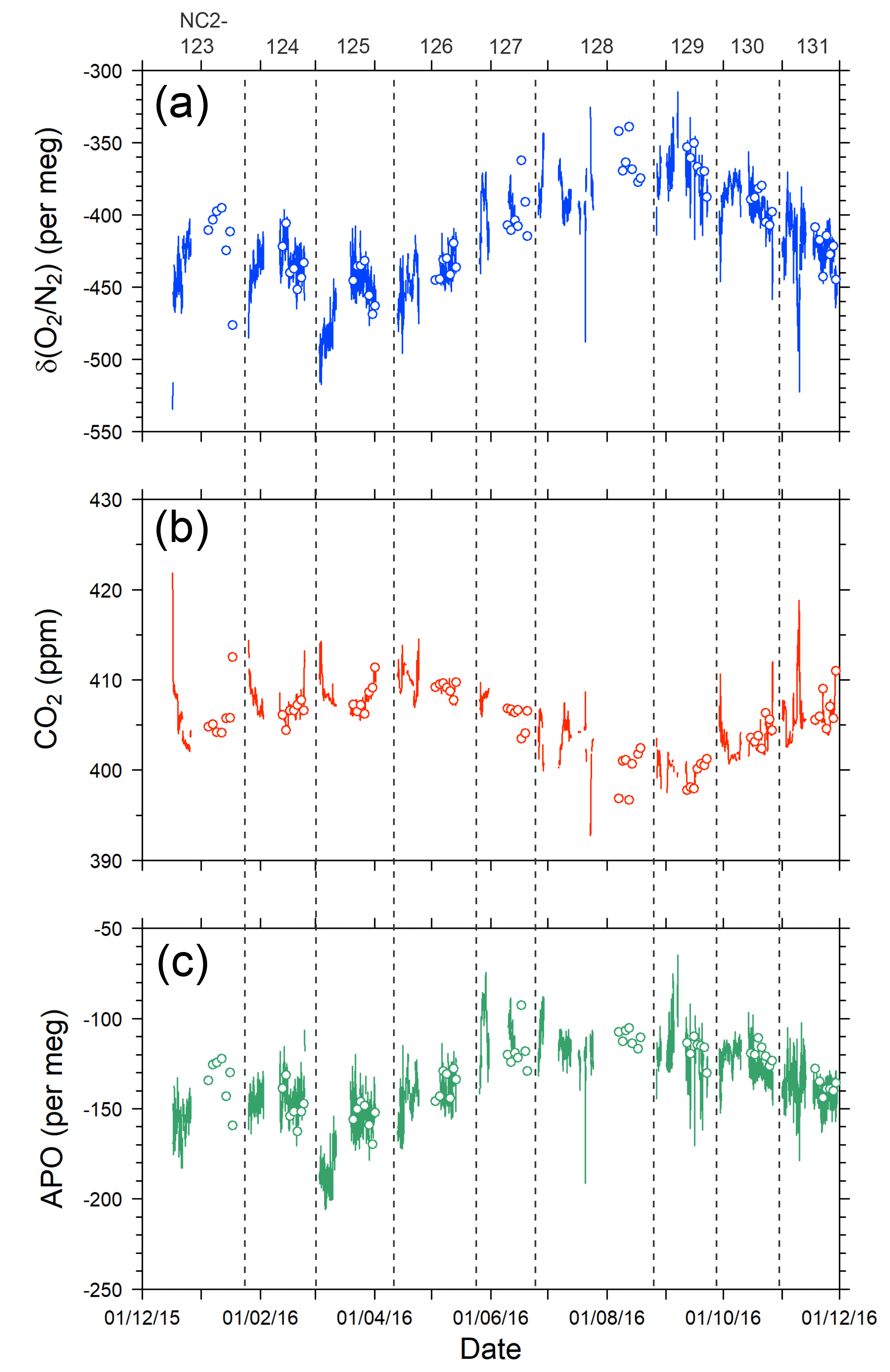
Figure 9Time series of (a) δ(O2 ∕ N2), (b) CO2, and (c) APO during the 1-year period from December 2015 to November 2016. Lines indicate continuous observation, and circles indicate flask measurements. Data obtained near the coasts of Japan and North America are excluded. Vertical dashed lines separate each cruise and the top labels represent cruise numbers.
The time series of the in situ data shown in Fig. 9 do not necessarily show smooth changes, which may be partly attributed to the fact that the onboard observations were conducted in the broad area of the North Pacific. For example, the APO values are relatively low (< −180 per meg) during the eastbound voyage NC2-125 in early March and high (> −100 per meg) during the eastbound voyage NC2-127 in late May. The longitudinal distributions of the 5 h running average of APO for the individual round-trip cruises are depicted in Fig. 8b, which clearly shows these anomalously low (blue line of NC2-125) and high (light blue line of NC2-127) APO distributions. Preliminary analyses of the cause of these anomalies point to atmospheric transport and the expected air–sea gas exchanges in the source regions. Detailed discussions of the anomalous changes are beyond the scope of this paper and will be presented in a future publication.
3.3 Distribution of seasonal cycles in the North Pacific
We investigated the longitudinal distribution of the seasonal amplitude of APO in the middle latitudes of the North Pacific using 1 year of in situ data within the area of 29–45∘ N and 140∘ E–130∘ W (Fig. 8a). The in situ data were binned into 10 longitudinal bands (140–150∘ E, 150–160∘ E, …, 140–130∘ W) and fitted to the following function using a least-squares method:
where a1 is a detrending coefficient (−7.9 per meg yr−1) determined from the APO values measured from the flask samples collected aboard NC2 during the 2-year period 2014–2016.
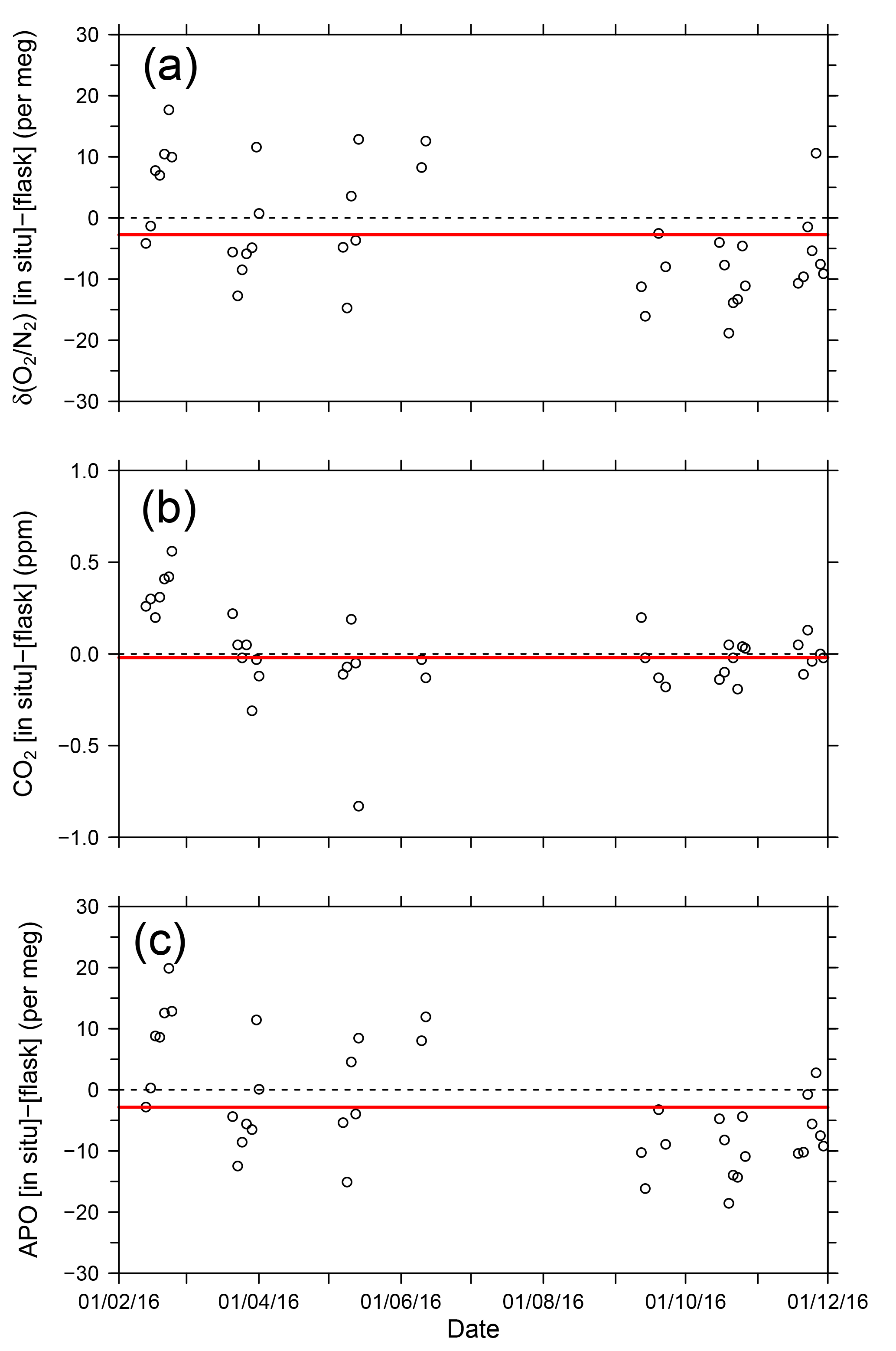
Figure 10Time series of differences in (a) δ(O2 ∕ N2), (b) CO2, and (c) APO between the in situ measurements and flask measurements (in situ–flask). The red lines show average values.
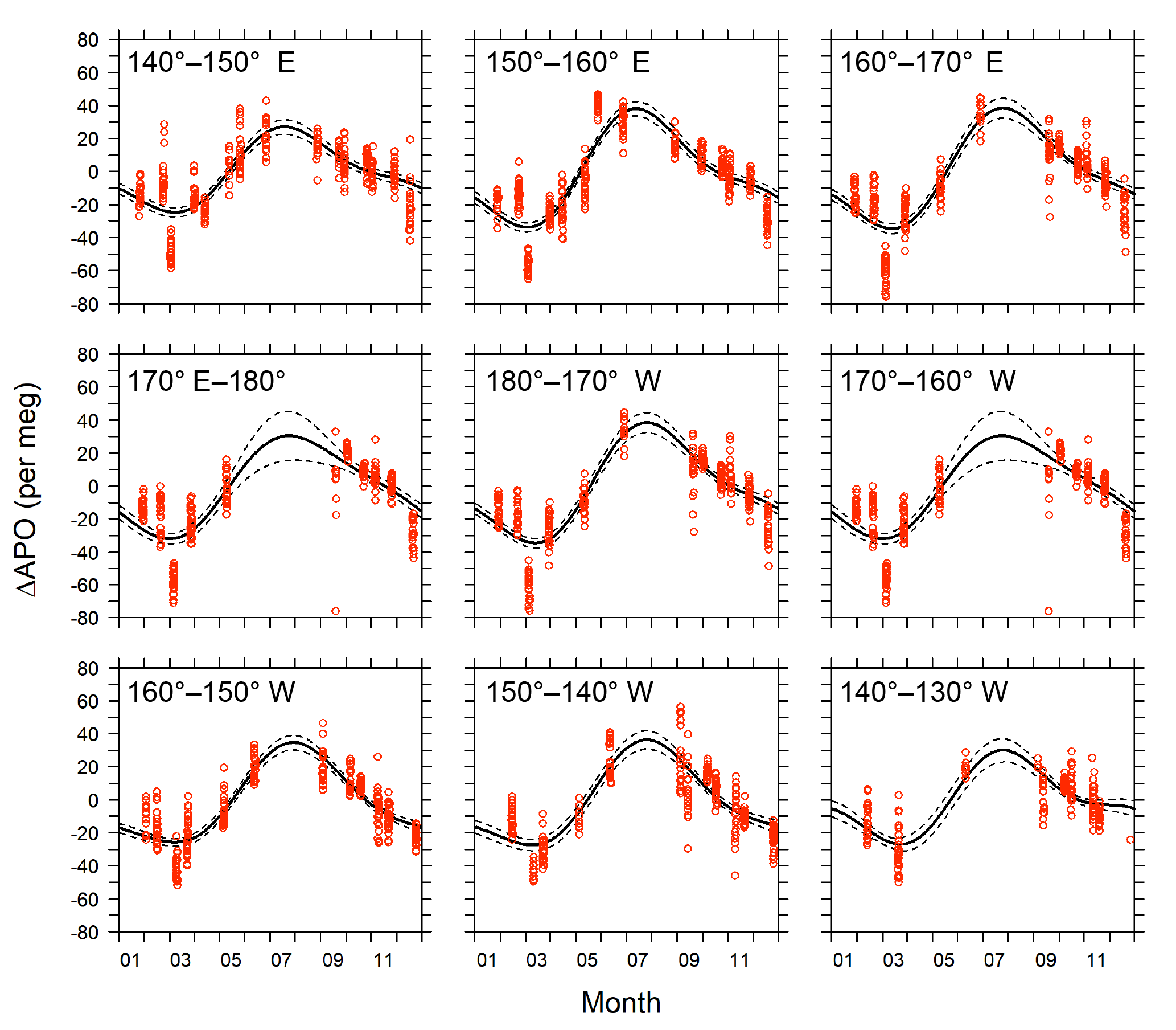
Figure 11Detrended seasonal variations in APO for the 10 longitudinal bins within the rectangular area of 29–45∘ N and 140∘ E–130∘ W. Red circles represent hourly averages of in situ APO data. Solid lines are average seasonal cycles determined by a least-squares method. Dashed lines indicate 95 % confidence intervals determined by a linear prediction model.
The detrended in situ data for the individual longitudinal bins and the fitted average seasonal cycles are shown in Fig. 11. The APO seasonal amplitudes for the 10 bins are plotted along with the longitude in Fig. 12a. For comparison, we also plot the seasonal amplitudes of APO in the North Pacific reported by Tohjima et al. (2012). In the previous study, APO data from the flask samples collected in the Pacific during the period from 2002 to 2008 were binned into several rectangular regions and the seasonal cycles for the binned data were examined in the same way as in this study. The seasonal amplitudes in the previous study varied from 20 per meg to 110 per meg, while those in this study varied from 51 per meg to 73 per meg. The difference in the seasonal amplitudes seems to be explained by the dependence of the latitudinal distribution, which is clearly shown in Fig. 12b, in which all the seasonal amplitudes shown in Fig. 12a are plotted along with the latitude. Such latitudinal dependence of the APO amplitude was previously pointed out for data from the western Pacific (Tohjima et al., 2005, 2012). On the other hand, this study reveals that the longitudinal variability in the seasonal amplitude of APO in the North Pacific is rather small. This preliminary analysis suggests that the temporally and spatially dense atmospheric O2 and CO2 data obtained from the in situ observations aboard NC2 will enhance our understanding of air–sea gas exchange in the North Pacific.
We developed a shipborne system to continuously measure atmospheric O2 and CO2 variations based on a fuel cell oxygen analyzer (Oxzilla II) and a nondispersive infrared CO2 analyzer (LI-840A). To reduce the consumption rate of the working reference gas and standard gases supplied from high-pressure cylinders, a relatively low flow rate of 10 cm3 min−1 was adopted for the measurement system. By keeping the flow rate and pressure of the system constant, we achieved precisions of 3.8 per meg for the O2 measurements and 0.1 ppm for the CO2 measurements in the laboratory.
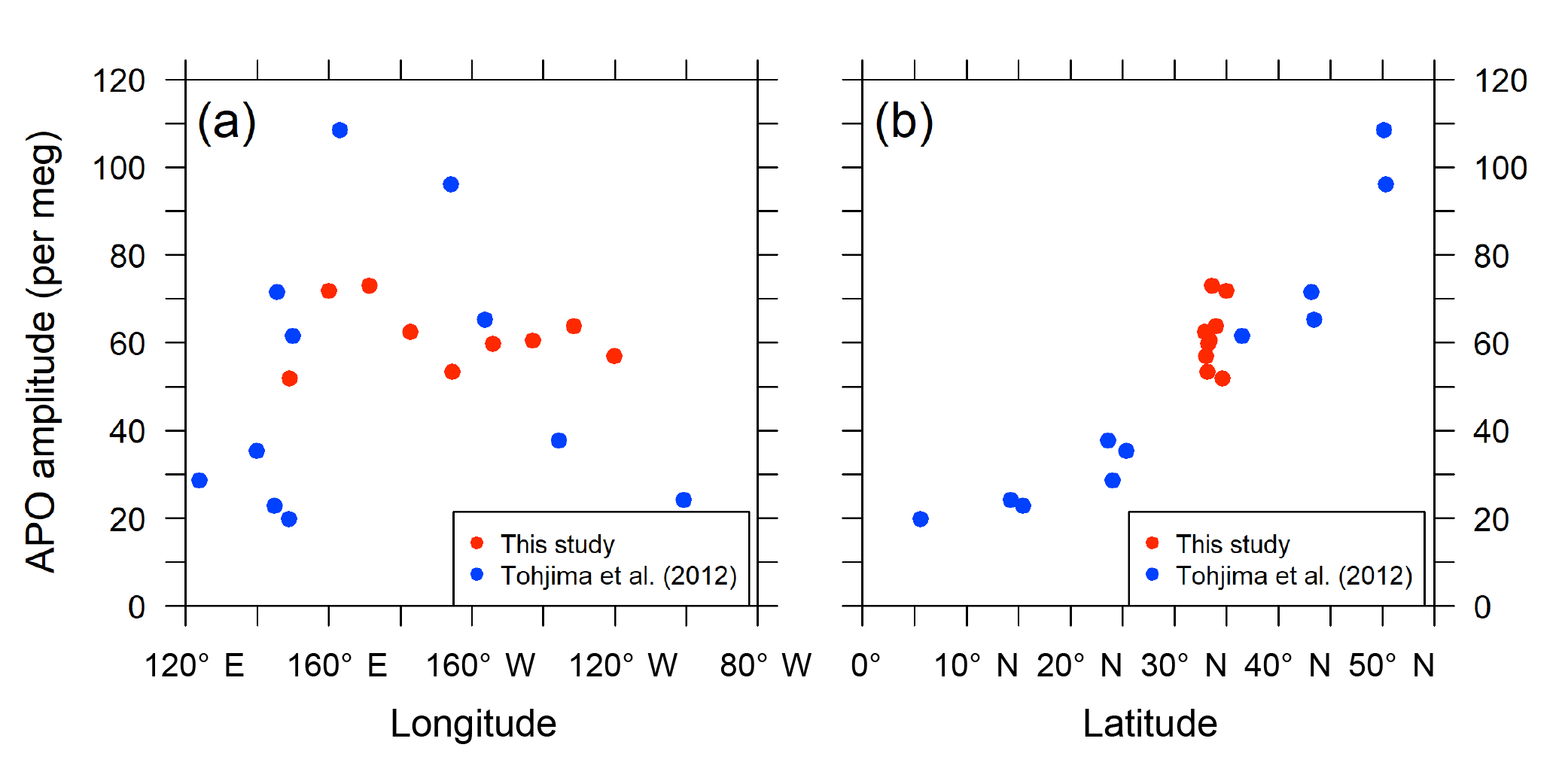
Figure 12Distribution of seasonal amplitudes of APO along with (a) longitude and (b) latitude in the North Pacific. The red symbols represent APO amplitudes of the in situ data from this study for individual longitudinal bins within middle latitudes (29–45∘ N and 140∘ E–130∘ W). The blue symbols represent APO amplitudes reported by Tohjima et al. (2012). The longitudes and latitudes in the plots are the average positions of the data within the individual bins.
We installed the measurement system on commercial cargo ship NC2 and started onboard continuous measurements in December 2015. We found that the ship motion significantly affected the output signal of the O2 analyzer; apparent wavy variations with amplitudes of more than 20 ppm and peak-to-peak periods of about 20 s were superimposed on the output signals during the voyage. Although this variation has not been eliminated yet, 1 h averaging considerably suppresses the variation associated with the ship motion because of the oscillatory nature of the apparent variations. From the comparison between the in situ measurements and simultaneously collected flask samples, we concluded that the uncertainties of δ(O2 ∕ N2) and CO2 mole fraction for the in situ measurements are about 9 per meg and about 0.3 ppm, respectively.
Using the in situ data obtained during the 1-year period from December 2015 to November 2016, we examined the longitudinal (140∘ E–130∘ W) distribution of seasonal APO amplitude at the middle latitudes (29–45∘ N) in the North Pacific. The amplitudes showed rather small longitudinal variability, with a range from 51 per meg to 73 per meg in comparison to the latitudinal variations reported by Tohjima et al. (2012). Although the problem related to the motion-induced degradation of O2 measurement precision has not been resolved, this study clearly demonstrated that in situ observations aboard cargo ships can extend the coverage of atmospheric O2 and CO2 data to a degree that flask sampling could never achieve.
The data presented in this article are available from Y. Tohjima (tohjima@nies.go.jp).
YT designed the study. YH carried out the shipboard measurements. KK and YH developed the measurement system. TM managed the measurements of the flask samples. SN managed the shipboard observation. YH wrote the paper with contributions and discussions from all coauthors.
The authors declare that they have no conflict of interest.
This article is part of the special issue “The 10th International Carbon Dioxide Conference (ICDC10) and the 19th WMO/IAEA Meeting on Carbon Dioxide, other Greenhouse Gases and Related Measurement Techniques (GGMT-2017) (AMT/ACP/BG/CP/ESD inter-journal SI)”. It is a result of the 19th WMO/IAEA Meeting on Carbon Dioxide, Other Greenhouse Gases, and Related Measurement Techniques (GGMT-2017), Empa Dübendorf, Switzerland, 27–31 August 2017.
We gratefully acknowledge the generous cooperation of Toyofuji Shipping Co.
and Kagoshima Senpaku Co. for providing us with the opportunity to make the onboard
atmospheric observations. Thanks are also expressed to the crew of the
New Century 2. We would like to thank Tomoyasu Yamada, Nobukazu Oda,
and other members of the Global Environmental Forum for their continued
support in maintaining the O2 and CO2 measurement system.
We thank Hisayo Sandanbata, Eri Matsuura, and Motoki Sasakawa of the NIES for
their continued support in the O2 and CO2 analysis of
flask samples. This work was financially supported by a Grant-in-Aid for
Scientific Research and in part by the Global Environmental Research
Coordination System from the Ministry of the Environment, Japan
(E1451).
Edited by: Martin Heimann
Reviewed by: two anonymous referees
Balkanski, Y., Monfray, P., Battle, M., and Heimann, M.: Ocean primary production derived from satellite data: an evaluation with atmospheric oxygen measurements, Global Biogeochem. Cy., 13, 257–271, 1999.
Battle, M., Bender, M. L., Tans, P. P., White, J. W. C., Ellis, J. T., Conway, T., and Francey, R. J.: Global carbon sinks and their variability inferred from atmospheric O2 and δ13C, Science, 287, 2467–2470, https://doi.org/10.1126/science.287.5462.2467, 2000.
Battle, M., Fletcher, S. M., Bender, M. L., Keeling, R. F., Manning, A. C., Gruber, N., Tnas, P. P., Hendricks, M. B., Ho, D. T., Simonds, C., Mika, R., and Paplawsky, B.: Atmospheric potential oxygen: New observations and their implications for some atmospheric and oceanic models, Global Biogeochem. Cy., 20, GB1010, https://doi.org/10.1029/2005GB002534, 2006.
Bender, M. L., Tans, P. P., Ellis, J. T., Orchardo, J., and Habfast, K.: A high precision isotope ratio mass spectrometry method for measuring the O2/N2 ratio of air, Geochim. Cosmochim. Ac., 58, 4751–4758, 1994.
Bopp, L., Le Quere, C., Heimann, M., Manning, A. C., and Monfray, P.: Climate-induced oceanic oxygen fluxes: Implications for the contemporary carbon budget, Global Biogeochem. Cy., 16, 1022, https://doi.org/10.1029/2001GB001445, 2002.
Goto, D., Morimoto, S., Ishidoya, S., Ogi, A., Aoki, S., and Nakazawa, T.: Development of a High Precision Continuous Measurement System for the Atmospheric O2/N2 Ratio and Its Application at Aobayama, Sendai, Japan, J. Meteorol. Soc. Jpn., 91, 179–192, https://doi.org/10.2151/jmsj.2013-206, 2013.
Ishidoya, S., Morimoto, S., Aoki, S., Taguchi, S., Goto, D., Murayama, S., and Nakazawa, T.: Oceanic and terrestrial biospheric CO2 uptake estimated from atmospheric potential oxygen observed at Ny-Ålesund, Svalbard, and Syowa, Antarctica, Tellus B, 64, 18924, https://doi.org/10.3402/tellusb.v64i0.18924, 2012.
Keeling, R. F.: Development of an interferometric oxygen analyzer for precise measurement of the atmospheric O2 mole fraction, PhD thesis, Harvard Univ., Cambridge, USA, 178 pp., 1988.
Keeling, R. F. and Garcia, H. E.: The change in oceanic O2 inventory associated with recent global warming, P. Natl. Acad. Sci. USA, 99, 7848–7853, https://doi.org/10.1073/pnas.122154899, 2002.
Keeling, R. F. and Manning, A. C.: Studies of recent changes in atmospheric O2 content, Treatise on Geochemistry: Second Edition, 385–404, ISBN9780080983004, 2014.
Keeling, R. F. and Shertz, S. R.: Seasonal and interannual variations in atmospheric oxygen and implications for the global carbon cycle, Nature, 358, 723–727, 1992.
Keeling, R. F., Najjar, R. P., Bender, M. L., and Tans, P. P.: What atmospheric oxygen measurements can tell us about the global carbon cycle, Global Biogeochem. Cy., 7, 37–67, 1993.
Keeling, R. F., Manning, A. C., McEvoy, E. M., and Shertz, S. R.: Methods for measuring changes in atmospheric O2 concentration and their application in southern hemisphere air, J. Geophys. Res. 103, 3381–3397, 1998.
Keeling, R. F., Manning, A. C., Paplawsky, W. J., and Cox, A. C.: On the long-term stability of reference gases for atmospheric O2/N2 and CO2 measurements, Tellus B, 59, 3–14, https://doi.org/10.1111/j.1600-0889.2006.00228x, 2007.
Lueker, T. J., Walker, S. J., Vollmer, M. K., Keeling, R. F., Nevison, C. D., and Weiss, F.: Coastal upwelling air-sea fluxes revealed in atmospheric observations of O2/N2, CO2 and N2O, Geophys. Res. Lett., 30, 1292, https://doi.org/10.1029/2002GL016615, 2003.
Machida, T., Tohjima, Y., Katsumata, K., and Mukai, H.: A new CO2 calibration scale based on gravimetric one-step dilution cylinders in National Institute for Environmental Studies-NIES 09 CO2 scale, in: Report of the 15thWMO Meeting of Experts on Carbon Dioxide Concentration and Related Tracer Measurement Techniques, edited by: Brand, W. A., Jena, Germany, September 7–10, 2009, WMO/GAW Report No. 194, WMO, Geneva, Switzerland, 114–118, 2011.
Manning, A. C. and Keeling, R. F.: Global oceanic and biotic carbon sinks from the Scripps atmospheric oxygen flask sampling network, Tellus B, 58, 95–116, https://doi.org/10.1111/j.1600-0889.2006.00175.x, 2006.
Manning, A. C., Keeling, R. F., and Severinghaus, J. P.: Precise atmospheric oxygen measurements with a paramagnetic oxygen analyzer, Global Biogeochem. Cy., 13, 1107–1115, 1999.
Naegler, T., Ciais, P., Orr, J. C., Aumont, O., and Rodenbeck, C.: On evaluating ocean models with atmospheric potential oxygen, Tellus B, 59, 138–156, https://doi.org/10.1111/j.1600-0889.2006.00197.x, 2007.
Nevison, C. D., Mahowald, N. M., Doney, S. C., Lima, I. D., and Cassar, N.: Impact of variable air-sea O2 and CO2 fluxes on atmospheric potential oxygen (APO) and land-ocean carbon sink partitioning, Biogeosciences, 5, 875–889, https://doi.org/10.5194/bg-5-875-2008, 2008.
Nevison, C. D., Keeling, R. F., Kahru, M., Manizza, M., Mitchell, B. G., and Cassar, N.: Estimating net community production in the Southern Ocean based on atmospheric potential oxygen and satellite ocean color data, Global Biogeochem. Cy., 26, GB1020, https://doi.org/10.1029/2011GB004040, 2012.
Nevison, C. D., Manizza, M., Keeling, R. F., Kahru, M., Bopp, L., Dunne, J., Tiputra, J., Ilyina, T., and Mitchell, B. G.: Evaluating the ocean biogeochemical components of Earth system models using atmospheric potential oxygen and ocean color data, Biogeosciences, 12, 193–208, https://doi.org/10.5194/bg-12-193-2015, 2015.
Nevison, C. D., Manizza, M., Keeling, R. F., Stephens, B. B., Bent, J. D., Dunne, J., Ilyina, T., Long, M., Reslandy, L., Tjiputra, J., and Yukimoto, S.: Evaluating CMIP ocean biogeochemistry and Southern Ocean carbon uptake using atmospheric potential oxygen: Present-day performance and future projection, Geohys. Res. Lett., 43, 2077–2085, https://doi.org/10.1002/2015GL067584, 2016.
Pickers, P.: New applications of continuous atmospheric O2 measurements: meridional transects across the Atlantic Ocean, and improved quantification of fossil fuel-derived CO2, PhD thesis, University of East Anglia, England, 262 pp., 2016.
Pickers, P. A., Manning, A. C., Sturges, W. T., Le Quéré, C., Mikaloff Fletcher, S. E., Wilson, P. A., and Etchells, A. J.: In situ measurements of atmospheric O2 and CO2 reveal an unexpected O2 signal over the tropical Atlantic Ocean, Global Biogeochem. Cy., 31, 1289–1305, https://doi.org/10.1002/2017GB005631, 2017.
Plattner, G. K., Joos, F., and Stocker, T. F.: Revision of the global carbon budget due to changing air-sea oxygen fluxes, Global Biogeochem. Cy., 16, 1096, https://doi.org/10.1029/2001GB001746, 2002.
Severinghaus, J. P.: Studies of the terrestrial O2 and carbon cycles in sand dune gases and in Biosphere 2, PhD thesis, Columbia Univ., New York, USA, 148 pp., 1995.
Stephens, B. B., Keeling, R. F., Heimann, M., Six, K. D., Murnane, R., and Caldeira, K.: Testing global ocean carbon cycle models using measurements of atmospheric O2 and CO2 concentration, Global Biogeochem. Cy., 12, 213–230, 1998.
Stephens, B. B., Keeling, R. F., and Paplawsky, W.: Shipboard measurements of atmospheric oxygen using a vacuum-ultraviolet absorption technique, Tellus B, 55, 857–878, https://doi.org/10.1046/j.1435-6935.2003.00075.x, 2003.
Stephens, B. B., Bakwin, P. S., Tans, P. P., Teclaw, R. M., and Baumann, D. D.: Application of a differential fuel-cell analyzer for measuring atmospheric oxygen variations, J. Atmos. Ocean. Tech., 24, 82–94, https://doi.org/10.1175/JTECH1959.1, 2007.
Thompson, R. L., Manning, A. C., Lowe, D. C., and Weatherburn, D. C.: A ship-based methodology for high precision atmospheric oxygen measurements and its application in the Southern Ocean region, Tellus B, 59, 643–653, https://doi.org/10.1111/j.1600-0889.2007.00292.x, 2007.
Tohjima, Y.: Method for measuring changes in the atmospheric O2/N2 ratio by a gas chromatograph equipped with a thermal conductivity detector, J. Geophys. Res., 105, 14575–14584, https://doi.org/10.1029/2000JD900057, 2000.
Tohjima, Y., Mukai, H., Machida, T., and Nojiri, Y.: Gas-chromatographic measurements of the atmospheric oxygen/nitrogen ratio at Hateruma Island and Cape Ochi-ishi, Japan, Geophys. Res. Lett., 30, 1653, https://doi.org/10.1029/2003GL017282, 2003.
Tohjima, Y., Machida, T., Watai, T., Akama, I., Amari, T., and Moriwaki, Y.: Preparation of gravimetric standards for measurements of atmospheric oxygen and reevaluation of atmospheric oxygen concentration, J. Geophys. Res., 110, D11302, https://doi.org/10.1029/2004JD005595, 2005.
Tohjima, Y., Mukai, H., Nojiri, Y., Yamagishi, H., and Machida, T.: Atmospheric O2/N2 measurements at two Japanese sites: Estimation of global oceanic and land biotic carbon sinks and analysis of the variations in atmospheric potential oxygen (APO), Tellus B, 60, 213–225, https://doi.org/10.1111/j.1600-0889.2007.00334.x, 2008.
Tohjima, Y., Minejima, C., Mukai, H., Machida, T., Yamagishi, H., and Nojiri, Y.: Analysis of seasonality and annual mean distribution of atmospheric potential oxygen (APO) in the Pacific region, Global Biogeochem. Cy., 26, GB4008, https://doi.org/10.1029/2011GB004110, 2012.
Tohjima, Y., Terao, Y., Mukai, H., Machida, T., Nojiri, Y., and Maksyutov, S.: ENSO-related variability in latitudinal distribution of annual mean atmospheric potential oxygen (APO) in the equatorial Western Pacific, Tellus B, 67, 1–15, https://doi.org/10.3402/tellusb.v67.25869, 2015.
van der Laan-Luijkx, I. T., Neubert, R. E. M., van der Laan, S., and Meijer, H. A. J.: Continuous measurements of atmospheric oxygen and carbon dioxide on a North Sea gas platform, Atmos. Meas. Tech., 3, 113–125, https://doi.org/10.5194/amt-3-113-2010, 2010.
Yamagishi, H., Tohjima, Y., Mukai, H., and Sasaoka, K.: Detection of regional scale sea-to-air oxygen emission related to spring bloom near Japan by using in-situ measurements of the atmospheric oxygen/nitrogen ratio, Atmos. Chem. Phys., 8, 3325–3335, https://doi.org/10.5194/acp-8-3325-2008, 2008.
Yamagishi, H., Tohjima, Y., Mukai, H., Nojiri, Y., Miyazaki, C., and Katsumata, K.: Observation of atmospheric oxygen/nitrogen ratio aboard a cargo ship using gas chromatography/thermal conductivity detector, J. Geophys. Res., 117, D04309, https://doi.org/10.1029/2011JD016939, 2012.