the Creative Commons Attribution 4.0 License.
the Creative Commons Attribution 4.0 License.
 | 25 Jun 2018
Comparison of ECHAM5/MESSy Atmospheric Chemistry (EMAC) simulations of the Arctic winter 2009/2010 and 2010/2011 with Envisat/MIPAS and Aura/MLS observations
Farahnaz Khosrawi
Oliver Kirner
Gabriele Stiller
Michael Höpfner
Michelle L. Santee
Sylvia Kellmann
Peter Braesicke
We present model simulations with the atmospheric chemistry–climate model ECHAM5/MESSy Atmospheric Chemistry (EMAC) nudged toward European Centre for Medium-Range Weather Forecasts (ECMWF) ERA-Interim reanalyses for the Arctic winters 2009/2010 and 2010/2011. This study is the first to perform an extensive assessment of the performance of the EMAC model for Arctic winters as previous studies have only made limited evaluations of EMAC simulations which also were mainly focused on the Antarctic winter stratosphere. We have chosen the two extreme Arctic winters 2009/2010 and 2010/2011 to evaluate the formation of polar stratospheric clouds (PSCs) and the representation of the chemistry and dynamics of the polar winter stratosphere in EMAC. The EMAC simulations are compared to observations by the Michelson Interferometer for Passive Atmospheric Soundings (Envisat/MIPAS) and the observations from the Aura Microwave Limb Sounder (Aura/MLS). The Arctic winter 2010/2011 was one of the coldest stratospheric winters on record, leading to the strongest depletion of ozone measured in the Arctic. The Arctic winter 2009/2010 was, from the climatological perspective, one of the warmest stratospheric winters on record. However, it was distinguished by an exceptionally cold stratosphere (colder than the climatological mean) from mid-December 2009 to mid-January 2010, leading to prolonged PSC formation and existence. Significant denitrification, the removal of HNO3 from the stratosphere by sedimentation of HNO3-containing polar stratospheric cloud particles, occurred in that winter. In our comparison, we focus on PSC formation and denitrification. The comparisons between EMAC simulations and satellite observations show that model and measurements compare well for these two Arctic winters (differences for HNO3 generally within ±20 %) and thus that EMAC nudged toward ECMWF ERA-Interim reanalyses is capable of giving a realistic representation of the evolution of PSCs and associated sequestration of gas-phase HNO3 in the polar winter stratosphere. However, simulated PSC volume densities are smaller than the ones derived from Envisat/MIPAS observations by a factor of 3–7. Further, PSCs in EMAC are not simulated as high up (in altitude) as they are observed. This underestimation of PSC volume density and vertical extension of the PSCs results in an underestimation of the vertical redistribution of HNO3 due to denitrification/re-nitrification. The differences found here between model simulations and observations stipulate further improvements in the EMAC set-up for simulating PSCs.
- Article
(8257 KB) - Full-text XML
- BibTeX
- EndNote


The severity of ozone destruction during polar winter in the lower stratosphere is dependent on the prevailing meteorology. During cold Arctic winters temperatures are sufficiently low to allow for the formation of polar stratospheric clouds (PSCs), which play a key role in stratospheric ozone destruction (Solomon et al., 1986; Crutzen and Arnold, 1986). In the polar spring, heterogeneous reactions take place on and within the PSC particles, which convert halogens from relatively inert reservoir species into forms which can destroy ozone efficiently (e.g. Peter, 1997; Solomon, 1999; Lowe and MacKenzie, 2008).
PSCs consist of liquid or solid particles and have according to their composition and physical state been classified into three different types: (1) supercooled ternary solution (STS), (2) nitric acid trihydrate (NAT), and (3) ice. Liquid PSC cloud particles (STS) form by the condensation of water vapour (H2O) and nitric acid (HNO3) on the liquid stratospheric background sulfate aerosol particles at temperatures 2–3 K below the NAT existence temperature TNAT (∼ 195 K at 50 hPa). For the formation of solid cloud particles (NAT and ice) much lower temperatures (slightly above or below the ice frost point Tice (∼ 188 K at 50 hPa)) are required (e.g. Carslaw et al., 1994; Koop et al., 1995). PSCs form at altitudes between 15 and 30 km. Denitrification, the permanent removal of HNO3 by sedimenting polar stratospheric cloud particles, limits the deactivation process of the ozone-destroying substances in springtime and thus leads to a prolongation of the ozone-destroying catalytic cycles.
The Arctic winters 2009/2010 and 2010/2011 were both exceptional. The Arctic winter 2010/2011 was one of the most persistently cold stratospheric winters on record, leading to the strongest depletion of ozone measured in the Arctic (Manney et al., 2011). The Arctic winter 2010/2011 has been well analysed, especially with respect to ozone loss (e.g. Manney et al., 2011; Sinnhuber et al., 2011; Arnone et al., 2012; Kuttippurath et al., 2012; Hommel et al., 2014). The dynamical perspective, and thus the exceptional dynamical conditions of this winter, was discussed in detail by Hurwitz et al. (2011), Isaksen et al. (2012), Strahan et al. (2013), and Shaw and Perlwitz (2014). Although the Arctic winter 2009/2010 was one of the warmest winters on record (Dörnbrack et al., 2012), it was distinguished by an exceptionally cold stratosphere (colder than the climatological mean) from mid-December 2009 to mid-January 2010, leading to prolonged PSC formation and significant denitrification (e.g. Khosrawi et al., 2011). The Arctic winter 2009/2010 has been well analysed both by measurements and model simulations. For example, detailed studies on denitrification during this winter were performed by Khosrawi et al. (2011) and on dehydration by Khaykin et al. (2013). An overview on the dynamical situation during this winter is given by Dörnbrack et al. (2012). Measurements were performed within the project RECONCILE (Reconciliation of essential parameters for an enhanced predictability of Arctic stratospheric ozone loss and its climate interactions), an intensive field campaign with the M55-Geophysica research aircraft. An overview of the measurements and results derived within this project is given in von Hobe et al. (2013).
Due to their importance in processes leading to ozone destruction in the polar winter stratosphere, an accurate representation of PSCs and binary sulfuric acid–water (background) aerosols is essential for the correct simulation of chlorine activation and polar ozone depletion in chemistry–climate models (CCMs). Here, we compare simulations of the Arctic winter stratosphere made with the submodel MSBM (Multi-phase Stratospheric Box Model, formerly PSC; Kirner et al., 2011, 2015) of the chemistry–climate model ECHAM5/MESSy Atmospheric Chemistry (EMAC; Jöckel et al., 2006, 2010) with observations from the Michelson Interferometer for Passive Atmospheric Soundings (Envisat/MIPAS) (Fischer and Oelhaf, 1996; Fischer et al., 2008) and the Aura Microwave Limb Sounder (Aura/MLS) (Waters et al., 2006). The submodel MSBM has been tested and optimized for the simulations of PSCs in the Antarctic (Kirner et al., 2011, 2015). EMAC simulation results of stratospheric nitrogen compounds and ozone were evaluated with Envisat/MIPAS observations by Brühl et al. (2007) for the Antarctic winter 2002.
The previous studies had their focus on the Antarctic, especially on ozone and chlorine activation. So far, no EMAC evaluation study has been performed focusing on the Arctic stratosphere. In this study, we test the representativeness of the EMAC simulations of PSCs and related quantities in the Arctic on the basis of simulations for the Arctic winters 2009/2010 and 2010/2011. In our study the focus is on PSC volume density, temperature, and HNO3. Further (qualitative) comparisons with additional trace gases (O3, ClO, and H2O) were performed in another study for the Arctic winter 2015/2016 (Khosrawi et al., 2017) where EMAC simulations were compared with observations from Aura/MLS and the Gimballed Limb Observer for Radiance Imaging of the Atmosphere (GLORIA) performed on board the High Altitude and LOng-range Research Aircraft (HALO).
2.1 The chemistry–climate model EMAC
The ECHAM5/MESSy Atmospheric Chemistry (EMAC) model is a numerical chemistry and climate simulation system that includes submodels describing tropospheric and middle-atmosphere processes and their interaction with oceans, land, and human influences (Jöckel et al., 2010). It uses the second version of the Modular Earth Submodel System (MESSy2) to link multi-institutional computer codes. The core atmospheric model is the fifth-generation European Centre Hamburg general circulation model (ECHAM5; Roeckner et al., 2006). For the present study we applied EMAC (ECHAM5 version 5.3.02, MESSy version 2.50) in T63L90MA resolution, i.e. with a spherical truncation of 63 (corresponding to a quadratic Gaussian grid of approximately in latitude and longitude) with 90 vertical hybrid pressure levels from the surface up to 0.01 hPa (approx. 80 km). A Newtonian relaxation technique of the prognostic variables temperature, vorticity, divergence, and (the logarithm of the) surface pressure above the boundary layer and below 1 hPa towards European Center for Medium-Range Weather Forecast (ECMWF) ERA-Interim reanalysis data (Dee et al., 2011) was applied, in order to nudge the model dynamics towards the observed meteorology.
Here we analyse an EMAC T63L90 simulation that was chemically initialized based on a previous simulation performed for the time period 1994 to 2010. The simulation was started on 1 January 2009 and continued until December 2011. The simulation includes a comprehensive chemistry set-up for the stratosphere and troposphere. Reaction rate coefficients for gas-phase reactions and absorption cross sections for photolysis are taken from Atkinson et al. (2007) and S. P. Sander et al. (2011). The applied model set-up comprised the following submodels: ONEMIS for “online” emissions of tracers and aerosols, OFFEMIS for “offline” emissions of tracers and aerosols, TNUDGE for tracer nudging (Kerkweg et al., 2006a), DDEP for dry deposition of trace gases and aerosols, SEDI for the sedimentation of aerosol particles (Kerkweg et al., 2006b), MECCA for the gas-phase chemistry (R. Sander et al., 2011), JVAL for the calculation of photolysis rates (Sander et al., 2014), SCAV for the scavenging and liquid-phase chemistry in cloud and precipitation (Tost et al., 2006a), CONVECT for the parameterization of convection (Tost et al., 2006b), LNOx for the source of NOx produced by lightning (Tost et al., 2007b), MSBM for the processes related to polar stratospheric clouds (Kirner et al., 2011), PTRAC for additional prognostic tracers (Jöckel et al., 2008), CVTRANS for convective tracer transport (Tost et al., 2006b), TROPOP for diagnosing the tropopause and boundary layer height (Jöckel et al., 2006), SORBIT for sampling model data along sun-synchronous satellite orbits (Jöckel et al., 2010), H2O for stratospheric water vapour (Jöckel et al., 2006), RAD for the radiation calculation (Jöckel et al., 2016), and CLOUD for calculating the cloud cover as well as cloud microphysics including precipitation (Tost et al., 2007a).
The submodel MSBM simulates the number densities, mean radii, and surface areas of sulfuric acid aerosols and the different polar stratospheric cloud particles (STS, NAT, and ice). The formation of STS particles is calculated through the uptake of HNO3 and H2O on the liquid binary sulfuric acid–water particles (Carslaw et al., 1995). Ice particles are assumed to form homogeneously at temperatures below the ice frost point temperature. For the calculation of the formation of solid particles a thermodynamic approach based on the equilibrium between the gas phase and the solid phase is assumed (e.g. Chipperfield, 1999). The vapour pressure over ice and NAT are calculated according to the parameterizations given in Marti and Mauersberger (1993) and Hanson and Mauersberger (1988), respectively. For the simulation of NAT particles two parameterizations are included in the submodel MSBM, one based on the heterogeneous formation of NAT on ice (“thermodynamical NAT parameterization”) and one based on the homogeneous formation of NAT (“kinetic growth NAT parameterization”). The “thermodynamical” NAT parameterization assumes an instantaneous thermodynamical equilibrium, while the “kinetic” parameterization is based on the growth and sedimentation algorithm given by Carslaw et al. (2002) and van den Broek et al. (2004). We use the kinetic growth parameterization in our EMAC simulation. NAT formation takes place as soon as a supercooling of 3 K below the NAT existence temperature (TNAT) is reached. A comprehensive description of the submodel MSBM can be found in Kirner et al. (2011).
2.2 Envisat/MIPAS
MIPAS is a middle-infrared Fourier transform spectrometer. MIPAS was launched in March 2002 on board Envisat and was operational until the sudden loss of contact with Envisat on 8 April 2012. MIPAS measured the atmospheric emission spectrum in the limb-sounding geometry. MIPAS operated in its nominal observation mode from June 2002 to March 2004. Measurements during this time period were performed in its full-spectral-resolution measurement mode with a designated spectral resolution of 0.035 cm−1. Measurements were performed covering the altitude range from the mesosphere to the troposphere with a high vertical resolution (about 3 km in the stratosphere). After a failure of the interferometer slide at the end of March 2004, MIPAS resumed measurements in January 2005 with a reduced spectral resolution of 0.0625 cm−1 but with improved spatial resolution. Data products of Envisat/MIPAS include 30 trace species – e.g. H2O, O3, HNO3, CH4, N2O, and NO2 – as well as temperature (Fischer and Oelhaf, 1996; Fischer et al., 2008). Here, the Envisat/MIPAS HNO3 and temperature data version V5H_HNO3_20 and V5H_T_20 and V5R_HNO3_224/225 and V5R_T_220/221 (nominal mode) derived with the IMK/IAA retrieval processor covering the periods July 2002–March 2003 and January 2005–April 2012, respectively, have been used (updated version of the retrieval as described in Milz et al., 2009, and von Clarmann et al., 2009). Comparison of the MIPAS HNO3 data product with satellite measurements from Odin/SMR (Odin/Sub-Millimetre Radiometer), ADEOS/ILAS-II (Advanced Earth Observing Satellite/Improved Limb Atmospheric Spectrometer), SCISAT/ACE-FTS (SCISAT/Atmospheric Chemistry Experiment–Fourier Transform Spectrometer), and the Envisat/MIPAS ESA (European Space Agency) product showed good agreement, and differences were generally within ±0.5 ppbv (Wang et al., 2007; Wolff et al., 2008). Differences between MIPAS HNO3 and the balloon-borne version of MIPAS (MIPAS-B) and the infrared spectrometer MkIV were even smaller, generally less than 0.5 ppbv throughout the altitude range up to 38 km. However, at high latitudes differences can increase up to 1–2 ppbv between 22 and 26 km due to the large horizontal inhomogeneity of HNO3 near the vortex boundary (Wang et al., 2007). Further comparisons of MIPAS data with other observations as well as application of the MIPAS HNO3 data to Antarctic studies can be found in Stiller et al. (2005) and Mengistu Tsidu et al. (2005). In addition to the HNO3 and temperature data, the MIPAS PSC data V5R_PSCVD_120_220 is used. This new MIPAS retrieval product of PSC volume density profiles has been derived recently (Höpfner et al., 2018). The retrieval procedure is similar to that described in Höpfner et al. (2006) but optimized such that the effect of different PSC types and sizes (e.g. Höpfner, 2004) on the estimated volume density is minimized. For each MIPAS limb scan this data set provides two profiles of PSC volume densities on a standard altitude grid of 1 km. These profiles indicate the range of possible values of volume density which are compatible with the MIPAS radiances under different assumptions for particle size. The typical vertical resolution of the retrieval is about 3–4 km.
2.3 Aura/MLS
The Microwave Limb Sounder (MLS) on the Earth Observing System Aura satellite was launched in July 2004. The Aura/MLS instrument is an advanced successor to the MLS instrument on the Upper Atmosphere Research Satellite (UARS). MLS is a limb-sounding instrument that measures the thermal emission at millimetre and submillimetre wavelengths using seven radiometers to cover five broad spectral regions (Waters et al., 2006). Measurements are performed from the surface to 90 km with a daily global latitude coverage from 82∘ S to 82∘ N. Here, we use Aura/MLS version v4.2 HNO3 and temperature data. The data screening criteria given by Livesey et al. (2017) have been applied to the data. A detailed assessment of the quality and reliability of the Aura/MLS v2.2 HNO3 measurements can be found in Santee et al. (2007). The HNO3 in v4.2 has been significantly improved compared to v2.2. In particular, the low bias in the stratosphere has been largely eliminated. Measurements of v4.2 HNO3 are performed with a horizontal resolution of 400–500 km and a vertical resolution of 3–4 km over most of the vertical range. In the lower stratosphere, the precision and systematic uncertainty for HNO3 are estimated to be 0.6 ppbv and 1.0–1.5 ppbv (2σ estimates), respectively (Livesey et al., 2017). The MLS v4.2 temperatures are similar to both the v3.3 and the v2.2 temperatures described in the validation study by Schwartz et al. (2008). MLS v4.2 temperatures have a ∼ −1 K bias with respect to correlative measurements in the troposphere and stratosphere. Further, in the MLS temperatures persistent, vertically oscillating biases with respect to analysis and correlative measurements have been found in the troposphere and stratosphere (see Livesey et al., 2017, for more details).
In the following a short description of the characteristics of the 2009/2010 and 2010/2011 Arctic winters considered in this study will be given. The Arctic winter 2010/2011 was one of the most persistently cold stratospheric winters on record. The prevailing cold temperatures in the stratosphere led to considerable denitrification and the strongest depletion of ozone measured in the Arctic (Manney et al., 2011). The Arctic winter 2009/2010, on the other hand, was rather warm in the climatological sense but was distinguished by an exceptionally cold stratosphere from mid-December 2009 to mid-January 2010 that led to prolonged PSC formation and significant denitrification (Dörnbrack et al., 2012; Khosrawi et al., 2011).
3.1 Arctic winter 2009/2010
The polar vortex formed in December and a Canadian warming in mid-December caused a splitting of the vortex into two parts. The colder part of the vortex was located over the Canadian Arctic and survived, resulting in a vortex recovery. The vortex then further cooled down through mid-January so that temperatures sufficiently low to allow solid PSCs to form were reached. The polar stratosphere was unusually cold from mid-December 2009 to the end of January 2010. A comparison of ECMWF ERA-Interim temperatures of the Arctic winters of the past half century showed that the 2009/2010 Arctic winter was one of the few winters with synoptic-scale temperatures below Tice (Pitts et al., 2011). Additionally, during mid-January orographic gravity waves were frequently excited by the flow over Greenland. A major warming in the second half of January (around 24 January) caused a displacement of the vortex to the European Arctic and also initiated the break-up of the vortex (Pitts et al., 2011; Dörnbrack et al., 2012).
In Pitts et al. (2011) a detailed description as well as examples of the PSCs observed by Cloud-Aerosol Lidar and Infrared Pathfinder Satellite Observations (CALIPSO) during the Arctic winter 2009/2010 is given. The measurements of PSCs by CALIPSO during that winter can be divided into four phases with distinctly different PSC optical characteristics: (1) 15–30 December 2009: the first phase was dominated by patchy, tenuous clouds consisting of liquid–NAT mixtures; (2) 31 December 2009 to 14 January 2010: the second phase was characterized by the occurrence of mountain wave ice clouds along the east coast of Greenland, enhanced numbers of mix 2 and mix 2 enhanced particles, and fully developed liquid STS clouds; (3) 15 to 21 January 2010: the third distinct phase occurred when temperatures synoptically cooled below Tice, resulting in synoptic-scale ice PSCs; and (4) 22 to 28 January 2010: the fourth and last phase was dominated by liquid STS clouds (Pitts et al., 2011).
3.2 Arctic winter 2010/2011
The Arctic winter 2010/2011 was one of the coldest stratospheric winters within the last 2 decades (Manney et al., 2011; Sinnhuber et al., 2011) and was characterized by an anomalously strong polar vortex with an atypically long cold period of stratospheric temperatures that was persistent from mid-December to mid-March (Manney et al., 2011). The polar vortex formed at the end of November 2010 and remained stable until the end of April. Due to minor warmings, the long cold period, lasting over 4 months, was interrupted by short warmer periods in the beginning of January, February, and March. In February and March, stratospheric temperatures were colder than in previous years of the last decade. The final warming during the 2010/2011 Arctic winter occurred later than usual, in mid-April (Arnone et al., 2012; Kuttippurath et al., 2012).
During the Arctic winter 2010/2011, the overall PSC occurrence frequency and area were exceptional for an Arctic winter as was shown by Manney et al. (2011) and confirmed in a recent study by Spang et al. (2018). The peak values of PSC area (in square kilometres) reached sizes comparable to June conditions in the Antarctic. Based on CALIPSO measurements, the PSC season during the 2010/2011 winter can be divided into four PSC phases according to the four cold phases that occurred in the stratosphere over the 4-month period from December 2010 to March 2011. The time periods of these four phases and the PSC types that occurred during each phase are as follows (Khosrawi et al., 2012): (1) 23 December 2010 to 8 January 2011: STS, mix 1 and mix 2, and ice clouds; (2) 20–28 January 2011: mainly mix 1 and mix 2 with some STS and ice; (3) 5–27 February 2011: STS, mix 1 and mix 2, and ice clouds; and (4) 5–19 March 2011: STS clouds (note that no CALIPSO data are available from 8 to 13 March 2011).
For our analysis the EMAC simulation with T63L90 resolution nudged toward ECMWF ERA-Interim reanalyses is used. The simulation was started on 1 January 2009 and continued until 31 December 2011. PSCs are calculated using the submodel MSBM (see Sect. 2.1). For the formation of NAT we used the kinetic NAT parameterization; thus NAT particles are formed as soon as the temperature drops below TNAT-3 K. The relative percentage differences between EMAC and the satellite measurements have been calculated by using the following equation: , with D in percent (%), where μ denotes the mixing ratio (e.g. HNO3) for EMAC and satellite measurements. The comparison is performed for two Arctic winters, 2009/2010 and 2010/2011. These two winters were quite different in their characteristics (Sect. 3) and are thus well suited for testing the model performance concerning chemistry and dynamics of the Arctic winter stratosphere. Comparisons of temperature, HNO3, and PSC volume densities are shown over the full vertical range (200–6 hPa) in time–pressure cross sections. In addition, for HNO3 we have chosen to highlight the 34 hPa level, where daily maps show the most pronounced gas-phase depletion features, and 50 hPa, where such signatures are largest in the time series of polar-cap-averaged HNO3 mixing ratios. In the present study, the focus is on PSC volume density, temperature, and HNO3. Further (qualitative) comparisons with additional trace gases (O3, ClO, and H2O) were performed in another study for the Arctic winter 2015/2016 (Khosrawi et al., 2017).
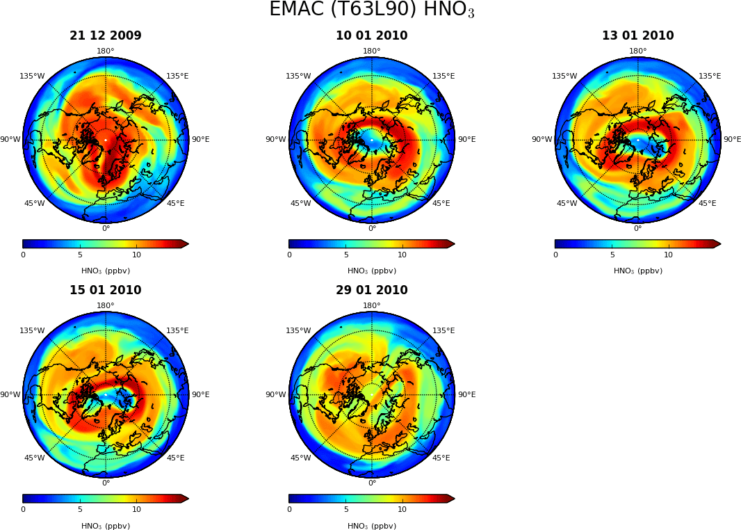
Figure 1Distribution of HNO3 as simulated with EMAC for 21 December 2009, 10, 13, 15, and 29 January 2010 at 34 hPa (≈ 21 km).
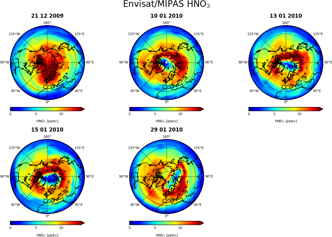
Figure 2Distribution of HNO3 as observed by Envisat/MIPAS on 21 December 2009, 10, 13, 15, and 29 January 2010 at at 21 km (∼ 34 hPa).
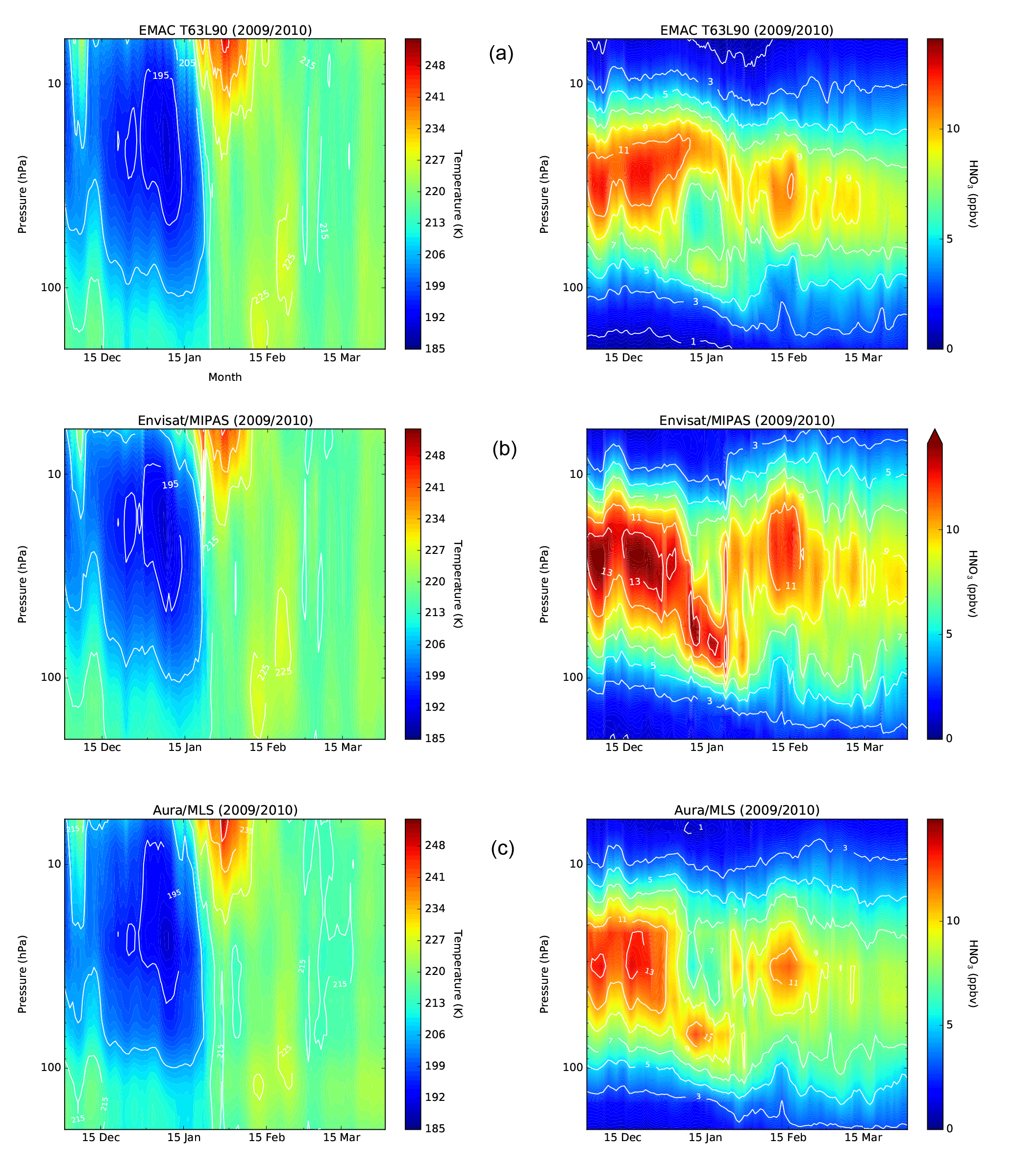
Figure 3Temporal evolution of temperature and HNO3 at northern high latitudes (70–90∘ N) as a function of pressure during the Arctic winter 2009/2010 (1 December 2009 to 31 March 2010). (a) EMAC, (b) Envisat/MIPAS, (c) Aura/MLS.
4.1 Simulation of the Arctic winter 2009/2010 and comparison to Envisat/MIPAS and Aura/MLS observations
Figure 1 shows the gas-phase distribution of HNO3 as simulated with EMAC for selected dates between 21 December 2009 and 29 January 2010 at 34 hPa (∼ 21 km). On 21 December 2009 the HNO3 distribution seems to be almost unchanged compared to the pre-winter distribution (not shown); thus HNO3 values are still high in the polar region. PSC formation has just started, but not much HNO3 has been taken up by the particles so far and thus removed from the gas phase. From early January onwards the HNO3 values start to decrease and reach very low values north of Scandinavia in mid-January (13 and 15 January), indicating a removal from the gas phase at 34 hPa (∼ 21 km). Due to the major warming and accompanying dissolution of PSCs, HNO3 values start to increase again toward the end of January.
In Fig. 2 the HNO3 distribution from Envisat/MIPAS is shown for the same dates as in Fig. 1. The EMAC simulation of the Arctic winter 2009/2010 compares generally well to the observations from Envisat/MIPAS. The same holds when EMAC simulations are compared to Aura/MLS observations (not shown). As in the EMAC simulation the observed HNO3 gas-phase distribution shows no signs of HNO3 removal on 21 December. This date falls into the first phase of PSC formation. During this time period (15–30 December) only patchy, tenuous clouds were observed by CALIPSO (Sect. 3.1), which did not significantly affect the HNO3 distribution at 34 hPa. Significant occurrence of PSCs was observed by CALIPSO from January onwards. Accordingly, gas-phase removal of HNO3 in PSCs is found in the Envisat/MIPAS observations from early January onwards and peaks towards mid-January. The simulation by EMAC shows the gas-phase depletion in the same areas as observed by Envisat/MIPAS. However, there are some minor differences between the EMAC simulations and the measurements from Envisat/MIPAS. On 15 January the HNO3 values simulated by EMAC are not as low as those observed by Envisat/MIPAS. Similar differences between EMAC and Envisat/MIPAS are found on 29 January 2010. Here the EMAC simulation also shows slightly higher HNO3 mixing ratios in the depleted area than was observed by Envisat/MIPAS.
In the following, time–pressure cross sections of temperature and HNO3 are considered to investigate how the EMAC simulations compare to the satellite observations during the course of the winter. Here, measurements from both satellites, Envisat/MIPAS and Aura/MLS, are considered. Figure 3 shows the temporal evolution of temperature and HNO3 from EMAC, Envisat/MIPAS, and Aura/MLS for the Arctic winter 2009/2010 (December 2009 to April 2010) at high latitudes (averaged over 70–90∘ N) as a function of pressure. The patterns of the temporal evolution of HNO3 derived from Envisat/MIPAS and Aura/MLS are generally similar; however, Envisat/MIPAS provides slightly higher HNO3 abundances than Aura/MLS (see e.g. Sheese et al., 2017, for a thorough comparison and discussion of the differences between Aura/MLS and Envisat/MIPAS). Note that the different sampling properties of the two instruments (with MIPAS not sensitive to gas-phase constituents in the presence of PSCs) should be taken into account (Millán et al., 2018).
The temperatures from EMAC nudged toward ECMWF ERA-Interim are in good agreement with the temperatures measured by Envisat/MIPAS and Aura/MLS. However, the warming in mid-January is simulated slightly more strongly in EMAC. Warm temperatures propagate further down into the stratosphere than observed by Envisat/MIPAS and Aura/MLS. Temperatures below 195 K occur in the region between 10 and 50 hPa (∼ 20–28 km) from mid-December to mid-January. Note that due to the nudging the simulated temperatures are quite close to those from ERA-Interim, but still some differences remain (see comparisons between EMAC, ERA-Interim, and satellite observations presented in Jöckel et al., 2006, 2016). The influence of gravity waves on temperature, which is measured by the satellites but still not fully resolved in the reanalyses data (and thus not reflected in the nudged model simulation), is e.g. one reason why differences between model simulations and observations are found, not only with regard to temperature but also with regard to PSCs (Höpfner et al., 2006).
In the simulated and observed HNO3 distribution gas-phase HNO3 is removed from the beginning of January onwards and remains low until the end of January. Although the EMAC simulation and the satellite observations from Envisat/MIPAS and Aura/MLS show removal of gas-phase HNO3 in accordance with the time and pressure levels where temperatures below 195 K are found, there are nevertheless obvious differences between model simulations and satellite observations. One prominent difference between EMAC HNO3 and the satellite observations is that EMAC shows a 2 ppbv lower maximum value in the HNO3 background distribution (early December). Otherwise the early-winter HNO3 distribution of EMAC compares well to Envisat/MIPAS and Aura/MLS concerning structure and temporal development. The same holds for the late-winter HNO3 distribution. However, this comparison shows that EMAC HNO3 seems generally 1–2 ppbv too low in early winter and throughout the PSC season. These too-low HNO3 mixing ratios in the EMAC simulation are also visible in the time series discussed below (Figs. 6 and 12).

Figure 4Volume density of all (liquid and solid) PSC particles (VPSC) in µm3 cm−3 as simulated with EMAC (a) and observed with Envisat/MIPAS lower limit (b) and Envisat/MIPAS upper limit (c) for the Arctic winter 2009/2010. Note the different colour bar scales between the Envisat/MIPAS and EMAC panels.
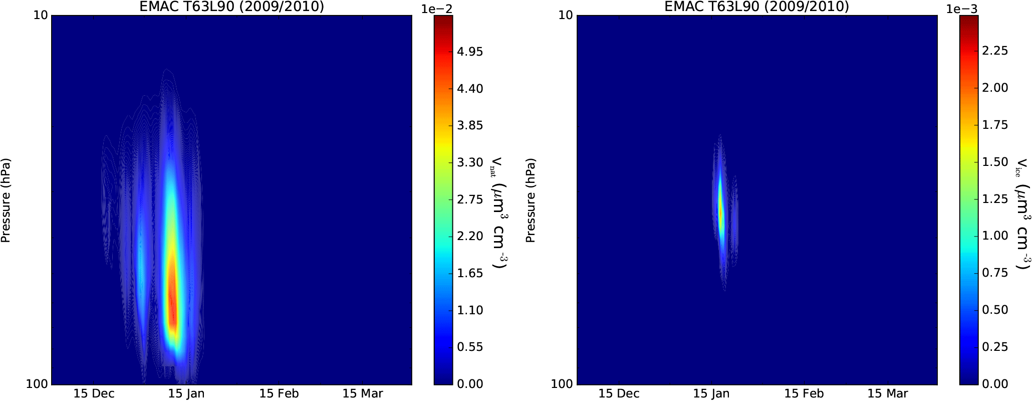
Figure 5Volume density of solid particles (VNAT and Vice) in µm3 cm−3 as simulated with EMAC for the Arctic winter 2009/2010.
Another prominent difference between the EMAC simulation and the observations by Envisat/MIPAS and Aura/MLS is found with the onset of HNO3 gas-phase removal by PSCs and throughout the PSC season (thus throughout January). Here, the satellite observations show HNO3 gas-phase removal which extends from the top of the high background values downwards. A downward-propagating tongue of high HNO3 is found below the depleted area, indicating vertical redistribution of HNO3 due to denitrification/re-nitrification. That the HNO3 gas-phase depletion in the Arctic winter 2009/2010 was permanent and thus led to a denitrification of the stratosphere in mid-January has been shown by e.g. Khosrawi et al. (2011). In the EMAC simulation the denitrified area is shifted towards lower pressure levels, and the simulated re-nitrification is not as strong as observed. This difference between EMAC and the satellite observations of Envisat/MIPAS and Aura/MLS in HNO3 throughout the PSC season arises because the simulated PSCs in EMAC differ from those observed by Envisat/MIPAS. This will be discussed in more detail in the following comparison of PSC volume densities.
Figures 4 and 5 show the temporal evolution of the volume density of PSC particles (VPSC in µm3 cm−3) and of NAT and ice particles (VNAT and Vice in µm3 cm−3) as a function of pressure as simulated with EMAC.1 In Fig. 4 additionally to the EMAC simulations the total PSC volume density VPSC derived from Envisat/MIPAS is shown. The MIPAS PSC data set provides two profiles of PSC volume densities that indicate the range of possible values, i.e. an upper and lower limit (see Sect. 2.2). In the Envisat/MIPAS observations the largest PSC volume density is found in January and reaches its maximum in mid-January. This is in agreement with PSC observations by CALIPSO during that winter (Sect. 3.1 and references therein). PSCs in EMAC start to form in mid-December (mainly NAT). In the beginning of January temperatures drop sufficiently low that ice formation is also briefly simulated.
The EMAC volume density compares well in terms of timing and structure to the volume density from Envisat/MIPAS. However, the EMAC PSC volume density is significantly smaller than the PSC volume density from Envisat/MIPAS (factor of 3 compared to the lower limit and 6–7 compared to the upper limit). This indicates that the amount of liquid particles is underestimated by EMAC. NAT formation in EMAC is already initiated at TNAT-3 K, which is a rather high threshold temperature for NAT formation. This is usually the temperature at which STS formation is initiated since for the formation of NAT particles usually temperatures lower than TNAT-3 K are required (Peter and Grooß, 2012; Lambert et al., 2016). However, this approach is commonly applied for simulating PSCs in atmospheric models (e.g. Wohltmann et al., 2013). As was discussed by Wohltmann et al. (2013), this approach technically results in NAT clouds being formed before STS clouds, and thus NAT formation occurs at the expense of STS since the NAT clouds consume all the available HNO3. This therefore results in an overestimation of NAT since in reality STS and NAT clouds are often observed at the same time (e.g. Pitts et al., 2011; Peter and Grooß, 2012).
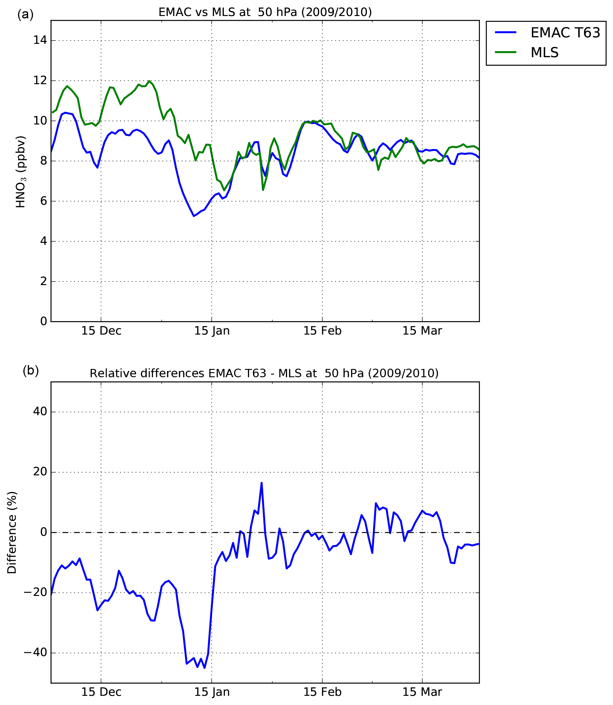
Figure 6(a) Time series of HNO3 (at 50 hPa) from EMAC (blue) and Aura/MLS (green) for the Arctic winter 2009/2010 (1 December 2009 to 31 March 2010, 70–90∘ N). (b) Relative differences of the EMAC–MLS time series.
Another difference between EMAC and Envisat/MIPAS is that EMAC does not simulate PSCs as high in altitude as they were observed with Envisat/MIPAS. This difference is also found when EMAC simulations are compared to CALIPSO observations, where PSCs are found up to 28 km (∼ 10 hPa; see Fig. 9 in Pitts et al., 2011); thus HNO3 in our EMAC simulation is not removed from the gas phase as high up as seen in the Envisat/MIPAS and Aura/MLS observations (Fig. 3). Strong re-nitrification is visible in the Envisat/MIPAS and Aura/MLS observations in mid- to late January but is not as strongly simulated with EMAC. This underestimation of re-nitrification in EMAC could be caused by the formation of too many small NAT particles that do not grow to the particle sizes that are needed to cause significant denitrification and thus re-nitrification below. To better understand the differences between simulated and observed PSCs, further studies are necessary and planned for the future.
In the following, the time series of HNO3 for the Arctic winter 2009/2010 (at 50 hPa, averaged over 70–90∘ N) derived from the EMAC simulation is compared with the one derived from the Aura/MLS observations (Fig. 6). Both time series show the high background HNO3 mixing ratios that are found at the beginning of the winter. Towards mid-January HNO3 mixing ratios decrease to 6 and 8 ppbv and then start to increase again after the final warming at the end of January. Due to denitrification during this winter (e.g. Khosrawi et al., 2011), the HNO3 mixing ratios remain lower than they were at the beginning of the winter before the start of the PSC season.
The absolute (not shown) and relative differences between the EMAC and Aura/MLS time series were calculated (Fig. 6). The comparison of the time series confirms the differences found when comparing the cross sections. EMAC HNO3 mixing ratios are generally 1–2 ppbv or up to 20 % lower than the ones observed by Aura/MLS during the PSC season (beginning of December to mid-January). The largest relative differences (up to 45 %) are found in mid-January, when the PSCs have their peak occurrence. The underestimation of HNO3 in the model simulation also affects chlorine activation and ozone loss, but other factors like the underestimation of transport in the model and inaccuracies in the partitioning between chlorine species at high solar zenith angles as discussed for the Arctic winter 2015/2016 in Khosrawi et al. (2017) also play a role.
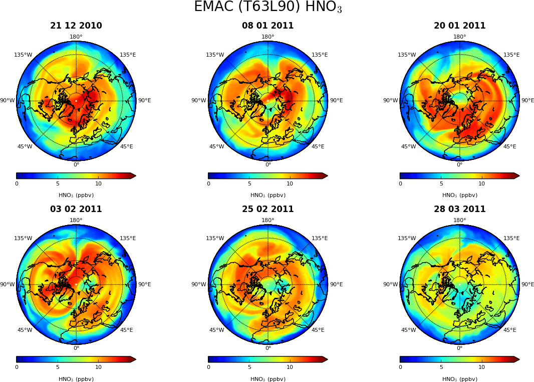
Figure 7Distribution of HNO3 as simulated with EMAC for 21 December 2010, 8 and 20 January 2011, 3 and 25 February 2011, and 28 March 2011 at 34 hPa (≈ 21 km).
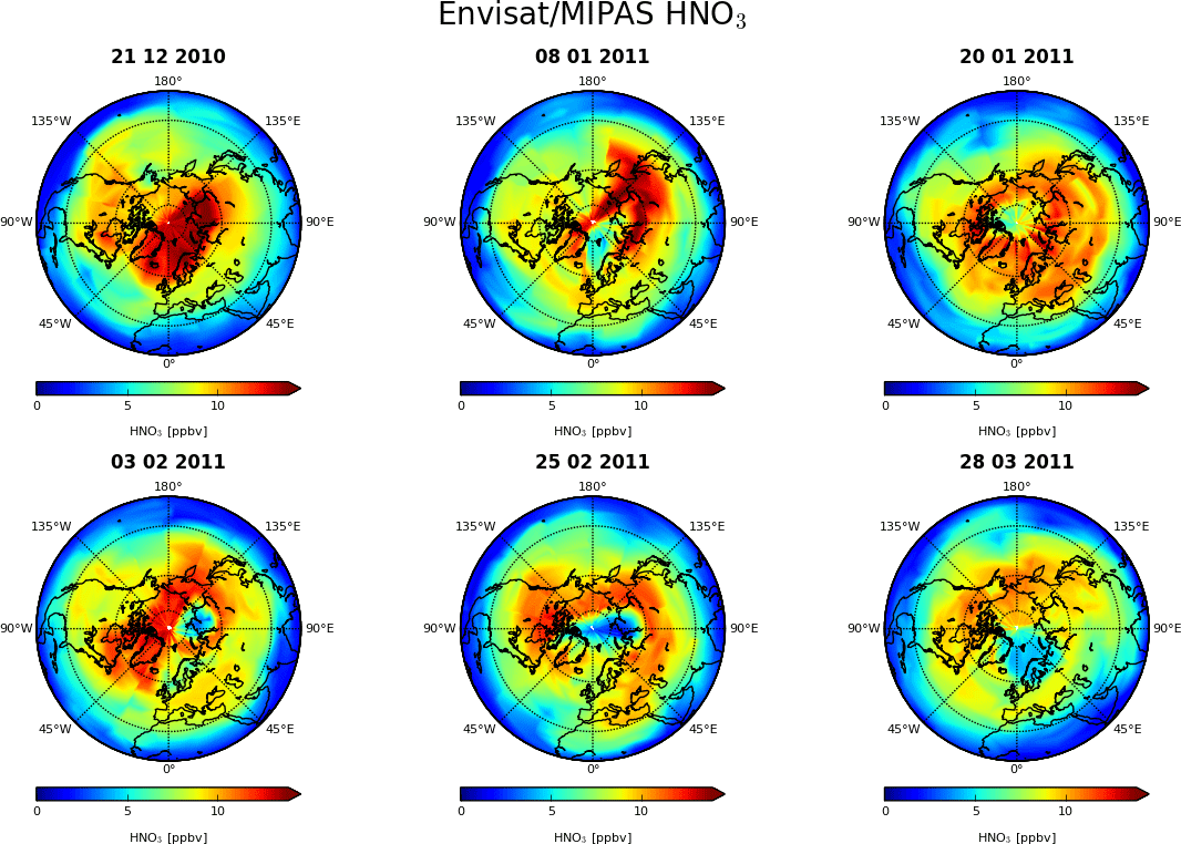
Figure 8Distribution of HNO3 as observed by Envisat/MIPAS for 21 December 2010, 8 and 20 January 2011, 3 and 25 February 2011, and 28 March 2011 at 21 km (∼ 34 hPa).
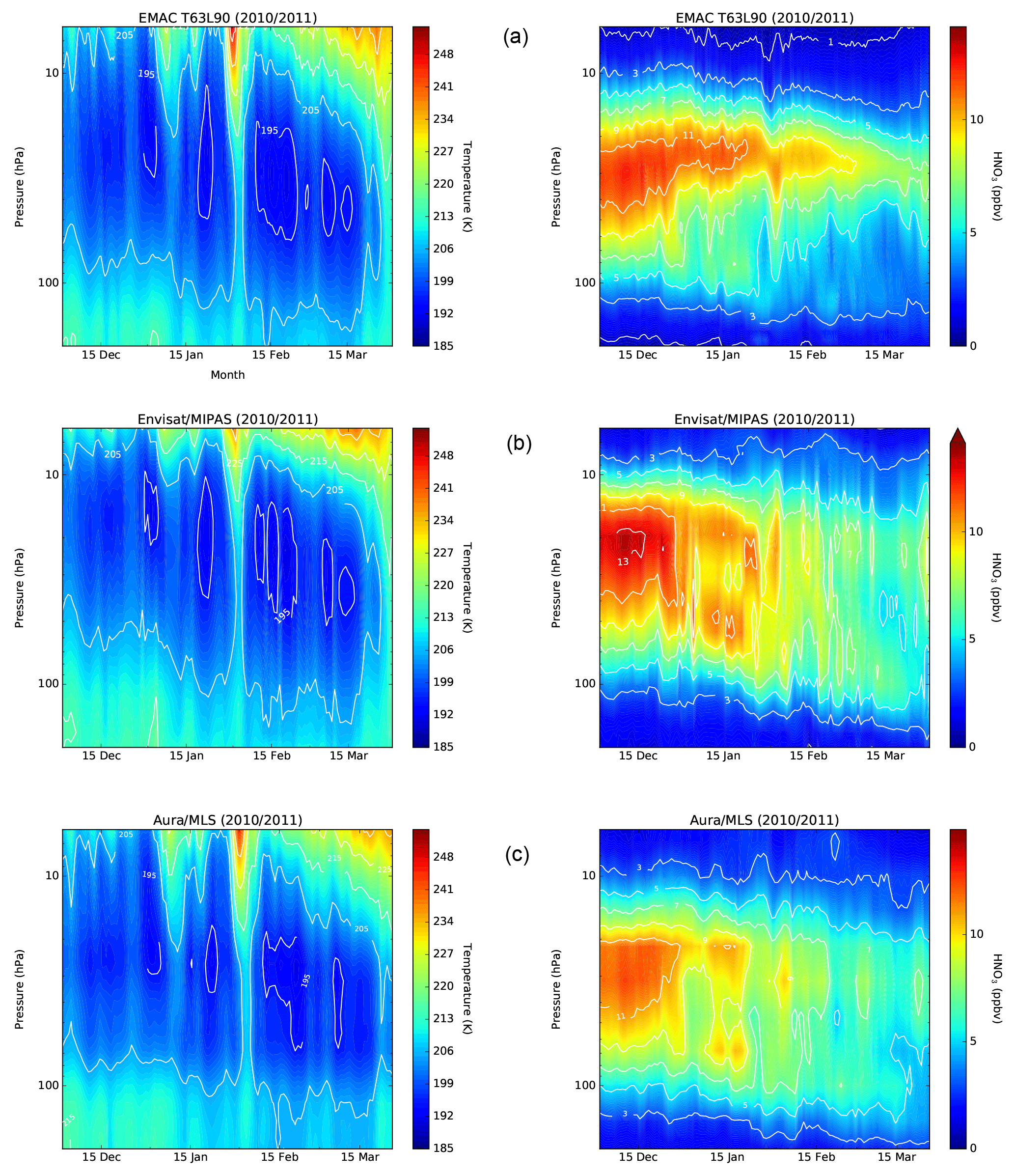
Figure 9Temporal evolution of temperature and HNO3 at northern high latitudes (70–90∘ N) as a function of pressure during the Arctic winter 2010/2011 (1 December 2010 to 31 March 2011). (a) EMAC, (b) Envisat/MIPAS, (c) Aura/MLS.
4.2 Simulation of the Arctic winter 2010/2011 and comparison to Envisat/MIPAS and Aura/MLS observations
As for the Arctic winter 2009/2010, we start with a comparison of daily maps of HNO3. Figure 7 shows the gas-phase distribution of HNO3 as simulated with EMAC for selected dates between 21 December 2010 and 28 March 2011 at 34 hPa (∼ 21 km). On 21 December 2010 the HNO3 distribution is still unperturbed by PSC formation. Onset of HNO3 removal is visible from 8 January onwards. On 26 January HNO3 mixing ratios reach a minimum (not shown). On 25 February and 28 March HNO3 mixing ratios have slightly recovered but remain lower than the pre-winter mixing ratios.
The HNO3 distribution as simulated with EMAC compares generally well with the HNO3 distribution measured during that winter by Envisat/MIPAS (Fig. 8). However, as was found for the Arctic winter 2009/2010, EMAC HNO3 background mixing ratios tend to be ∼ 2 ppbv lower than observed, and removal of HNO3 seems to be not as strong in the simulation as in the observations. Also during the Arctic winter 2010/2011 HNO3 was permanently removed from the stratosphere, thus leading to a strong denitrification of the Arctic stratosphere as has been shown in previous studies using observations from Aura/MLS, Odin/SMR, and Envisat/MIPAS (Manney et al., 2011; Khosrawi et al., 2012; Arnone et al., 2012). Thus, this indicates that in the EMAC simulation of the Arctic winter 2010/2011 denitrification/re-nitrification is also underestimated as will be discussed further below.
Differences in the daily maps that may be caused by transport processes in the model are found on 8 January and 3 February 2011. The Envisat/MIPAS (Fig. 8) and Aura/MLS (not shown) measurements on 8 January 2011 show an elongated area with low HNO3 stretching near the pole from north-east to south-west. In EMAC this area is simulated to be rather circular and thus has a smaller spatial extent than observed. On 3 February 2011 the EMAC simulation shows a dipole structure with two HNO3 minima, one over Russia and one over Greenland, which is not found in the satellite observations. In the Envisat/MIPAS and Aura/MLS observations only the minimum over Russia is observed. Around these two dates the stratosphere was dynamically quite active (Sect. 3.2). Minor warmings disturbed the stratosphere, and the differences in HNO3 seen here are most probably related to these. The minor warmings are simulated by EMAC with the correct timing but with a slightly different strength from that observed by Envisat/MIPAS and Aura/MLS as can be seen from the temperature distribution shown in Fig. 9. The cause of these differences may be related to model dynamics. In fact, an already-known feature in EMAC is that the downward transport is underestimated (Brühl et al., 2007; Khosrawi et al., 2009).
Figure 9 shows the temporal evolution of temperature and HNO3 from EMAC, Envisat/MIPAS, and Aura/MLS for the Arctic winter 2010/2011 (December 2010 to April 2011) at high latitudes (70–90∘ N) as a function of pressure. As for the Arctic winter 2009/2010 the simulated temperatures from EMAC nudged toward ECMWF ERA-Interim compare well with the temperatures measured by Envisat/MIPAS and Aura/MLS. However, the warmings in mid-January and mid-March are slightly more strongly simulated in EMAC than observed by Envisat/MIPAS. Another difference between the simulation and observations is that the area of temperatures lower than T<205 K extends further down in the EMAC simulation than in the Envisat/MIPAS observation (especially December to February), while the areas with temperatures T<195 hPa are shifted to higher pressure levels (lower altitudes). This difference in temperature probably also contributes to the differences between observed and measured PSCs (see below) and the underestimation of HNO3 removal we found in the EMAC simulation when comparing the daily maps.
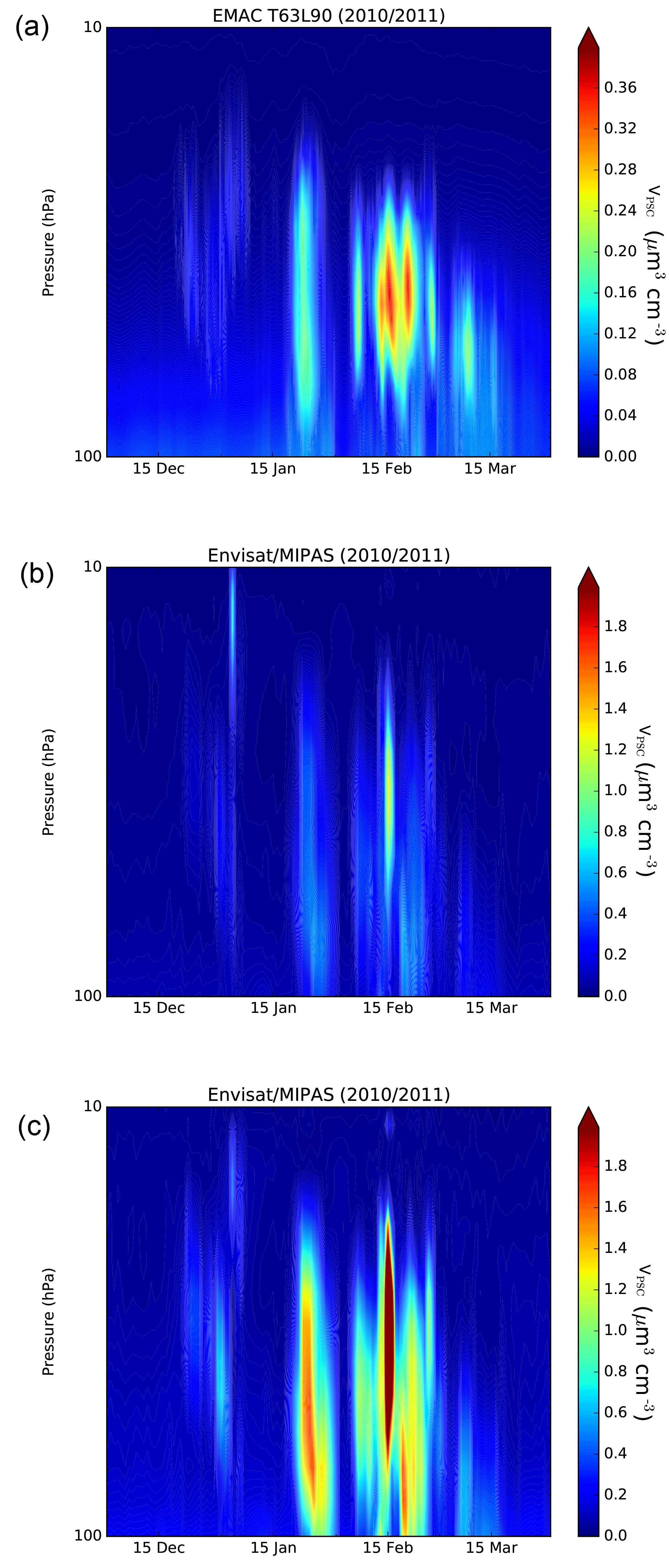
Figure 10Volume density of all (liquid and solid) PSC particles (VPSC) in µm3 cm−3 as simulated with EMAC (a) and observed with Envisat/MIPAS lower limit (b) and Envisat/MIPAS upper limit (c) for the Arctic winter 2010/2011. Note the different colour bar scales between the Envisat/MIPAS and EMAC panels.
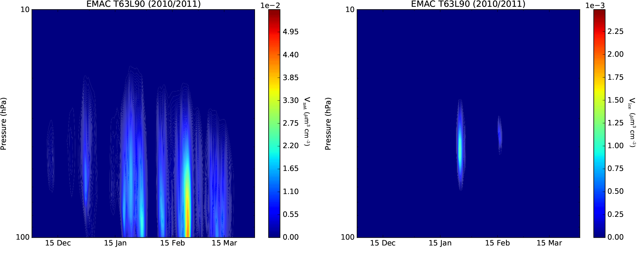
Figure 11Volume density of solid particles (VNAT and Vice) in µm3 cm−3 as simulated with EMAC for the Arctic winter 2010/2011.
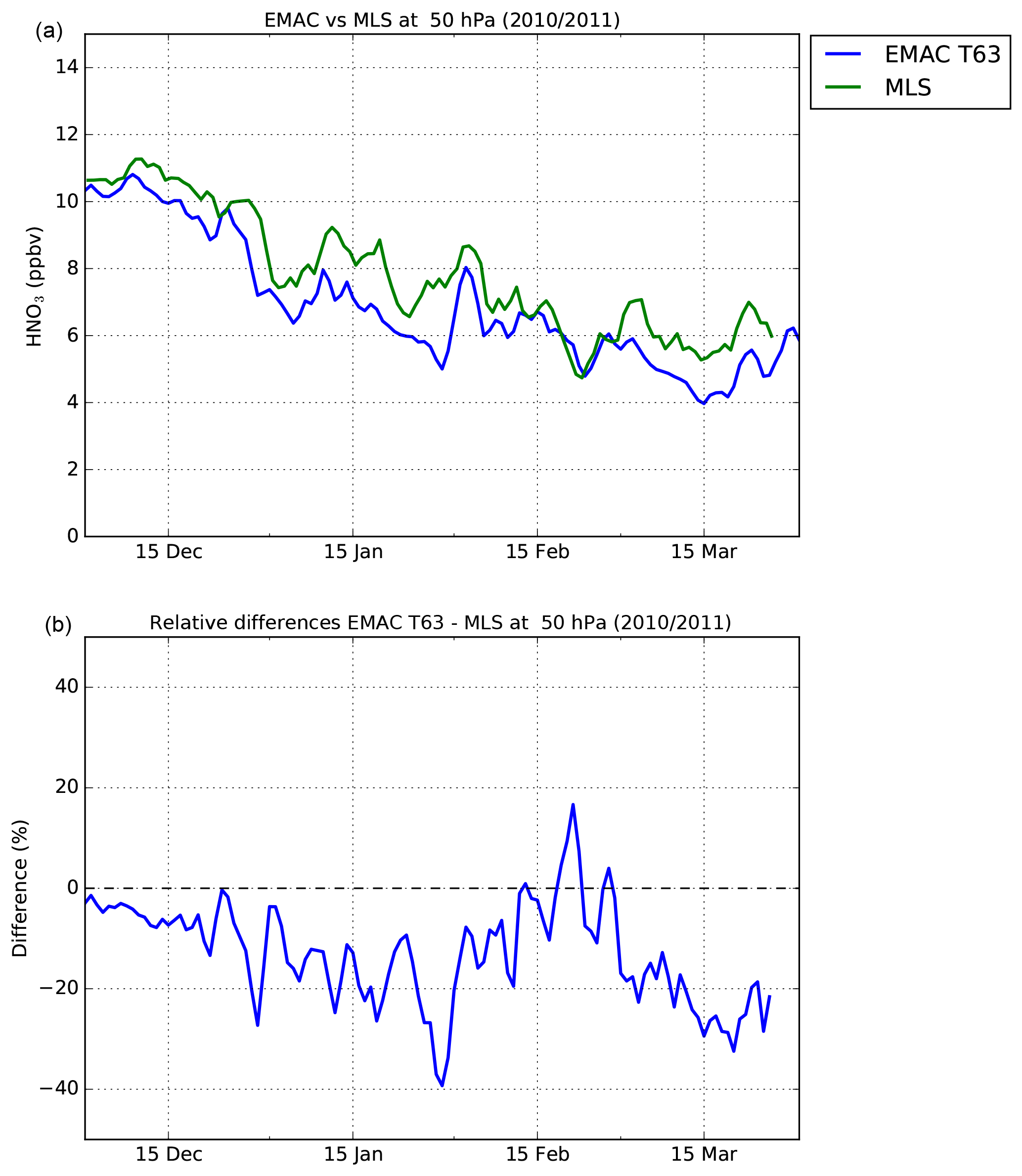
Figure 12(a) Time series of HNO3 (at 50 hPa) from EMAC (blue) and Aura/MLS (green) for the Arctic winter 2010/2011 (1 December 2011 to 31 March 2011, 70–90∘ N). (b) Relative differences of the EMAC–MLS time series.
As for the Arctic winter 2009/2010 a prominent difference between EMAC and the Envisat/MIPAS HNO3 for the Arctic winter 2010/2011 is that EMAC exhibits a ∼ 2 ppbv lower maximum mixing ratio in the HNO3 distribution (early December). However, contrary to the 2009/2010 winter, here the EMAC HNO3 mixing ratios are slightly higher compared to Aura/MLS. Otherwise the structure of the early-winter HNO3 distribution of EMAC is generally in agreement with Envisat/MIPAS and Aura/MLS. Larger differences (as already noted for the Arctic winter 2009/2010) are found throughout the PSC season. These differences are most probably caused by the differences between the simulated PSCs and those observed by Envisat/MIPAS (Fig. 10). Figures 10 and 11 show the temporal evolution of the volume density of PSC particles (VPSC in µm3 cm−3) and of NAT and ice particles (VNAT and Vice in µm3 cm−3) as a function of pressure as simulated with EMAC. In Fig. 10 additionally to the EMAC simulations the total PSC volume density VPSC derived from Envisat/MIPAS is shown.
In Envisat/MIPAS observations and the EMAC simulations the PSC season starts in mid-December 2010 and lasts until mid-March 2011. In accordance with the four stratospheric cold phases (Sect. 3.2), four phases of PSCs are observed by Envisat/MIPAS. These four PSC phases are also simulated with the correct timing by EMAC. In early winter the majority of particles simulated with EMAC are NAT since NAT formation is initiated at TNAT-3 K. Liquid STS particles are found in the EMAC simulation from mid-January to mid-March and ice particles at the end of January. The four PSC phases as simulated with EMAC (concerning time of occurrence of the PSCs and respective PSC types) are in agreement with CALIPSO (see Sect. 3.2 and Pitts and Poole, 2014) and Envisat/MIPAS (concerning time of occurrence of PSCs). However, again PSCs are not simulated as high up as measured by CALIPSO and Envisat/MIPAS. In the beginning of January, for example, PSCs are measured by CALIPSO up to 30 km. In EMAC PSCs are only found up to 15 hPa (approx. 26 km). The Envisat/MIPAS PSC volume also extends over a larger vertical range than the EMAC PSC volume, indicating (as in the Arctic winter 2010/2011) an underestimation of the PSC occurrence in the EMAC simulation. Another major difference between the EMAC and Envisat/MIPAS volume density is that the EMAC PSC volume is much smaller than Envisat/MIPAS (factor of 3–4 compared to the lower limit and 5 compared to the upper limit).
The above-discussed differences in the PSC volume are also reflected in the temporal evolution of the HNO3 distribution during the course of the winter (Fig. 9). A prominent difference between the HNO3 distribution simulated by EMAC and the HNO3 distributions measured by Envisat/MIPAS and Aura/MLS is that EMAC exhibits a slightly smaller background distribution and that the maximum in HNO3 is located at slightly higher pressure levels (lower altitudes). As PSCs form, gas-phase HNO3 is removed, but this removal occurs earlier and more strongly in EMAC, albeit restricted to 100 to 50 hPa, while the strong removal of HNO3 seen in the Envisat/MIPAS and Aura/MLS measurements from mid-January onwards extends over the area from 100 to 20 hPa. Further, the re-nitrification at ≈ 70 hPa (January) which is clearly seen in Envisat/MIPAS and Aura/MLS is not as clearly visible in the EMAC simulation, thus indicating an underestimation of re-nitrification in EMAC.
Similar differences in HNO3 as discussed above are found when comparing the time series derived from EMAC with the one derived from Aura/MLS (at 50 hPa, average over 70–90∘ N, Fig. 12). In terms of the temporal evolution the time series are in good agreement, but EMAC HNO3 is 1–2 ppbv lower during the time period when PSCs are present as was already found for the Arctic winter 2009/2010. At the beginning of the winter the HNO3 mixing ratios are in the range of about 10–11 ppbv and then decrease during the course of the winter to 6 ppbv due to sequestration in PSCs and denitrification. The relative differences are generally less than 20 % except for the time period when PSC occurrence has its maximum. Here, the differences increase briefly up to 40 %.
We simulated the Arctic winters 2009/2010 and 2010/2011 with the chemistry–climate model EMAC and compared the results to satellite observations from Envisat/MIPAS and Aura/MLS. We have chosen these two winters since both were quite extreme but nevertheless different in their chemical and dynamical characteristics. Thus, these two winters are well suited for testing the EMAC performance concerning chemistry and dynamics of the Arctic winter stratosphere. Previous similar but more limited studies focused on the Antarctic. In the study by Kirner et al. (2015), for example, only qualitative comparisons of ClO, O3, and HNO3 to Aura/MLS measurements were performed mainly based on multi-year averages. Our study is the first to perform an extensive assessment, both qualitative and quantitative, of the EMAC performance in the Arctic. Since we have chosen two extreme winters for this study, the differences derived here are the largest possible differences since not all Arctic winters are extreme. Nevertheless, the issues discussed here in the model performance remain, but differences between model simulation and observations throughout the PSC season are not as large for a rather warm winter, e.g. the Arctic winter 2008/2009. The EMAC simulation used in this study was performed with a T63L90 resolution. A Newtonian relaxation technique of the prognostic variables temperature, vorticity, divergence, and surface pressure towards ERA-Interim reanalyses was applied below 1 hPa, in order to nudge the model dynamics towards meteorological analyses.
The model simulations for the Arctic winters 2009/2010 and 2010/2011 compare well with measurements from Envisat/MIPAS and Aura/MLS, showing that EMAC is capable of giving a realistic representation of the Arctic winter stratosphere in terms of PSC formation and the HNO3 and temperature distribution. Especially for the (nudged) temperature a very good agreement between satellite measurements and model simulations was found throughout the winter season. However, the warmings were stronger in the simulations by EMAC than observed. The cause of these differences may be related to model dynamics. In fact, a well-known feature in EMAC is that downward transport is underestimated in the lower parts of the polar vortices (Brühl et al., 2007; Khosrawi et al., 2009), despite the model vorticity and divergence fields being nudged towards ECMWF ERA-Interim reanalyses. Further, as was discussed by Brühl et al. (2007), a too-tight subtropical barrier causing too-low N2O and too-high NOy in the middle stratosphere is simulated by EMAC. This indicates a need for further improvements of the model dynamics, particularly the forcing by gravity waves (Brühl et al., 2007). Furthermore, in a more recent study by Hoppe et al. (2014) it was shown that the standard flux-form semi-Lagrangian scheme used in EMAC may be too diffusive near the transport barriers and that the simulation results can be improved when a Lagrangian transport scheme is used instead.
Larger differences than for temperature were found concerning PSC formation/occurrence and the respective gas-phase distribution of HNO3. Here, the comparison between the PSC volume density as simulated with EMAC and the one derived from Envisat/MIPAS observations showed that the simulated PSC volume densities are much smaller than the observed ones (∼ 3–7 times smaller in 2009/2010 and ∼ 3–5 times smaller in 2010/2011). Since the PSC volume density is mainly determined by the liquid PSC volume density, this indicates an underestimation of liquid STS particles in the model. As commonly applied for simulating PSCs in atmospheric models (e.g. Wohltmann et al., 2013), NAT formation in EMAC is initiated at TNAT-3 K. This results in NAT clouds being formed before STS clouds, and thus NAT formation occurs at the expense of STS since the NAT clouds consume all the available HNO3. This therefore results in an overestimation of NAT since in reality STS and NAT clouds are often observed at the same time (e.g. Pitts et al., 2011; Peter and Grooß, 2012). Another difference between EMAC and Envisat/MIPAS PSC volume densities is that the EMAC PSCs have a smaller vertical extent than those observed by Envisat/MIPAS.
The differences we found in PSC volume densities are reflected in the HNO3 distribution. In 2009/2010 denitrification/re-nitrification is underestimated by EMAC, and the denitrified areas are shifted to lower pressure levels. Similar results are derived for the Arctic winter 2010/2011. For this winter PSCs are also not simulated as high up as measured and re-nitrification is underestimated, while denitrification occurs earlier and more strongly in EMAC than observed by Envisat/MIPAS and Aura/MLS. This underestimation of re-nitrification in EMAC may be caused by the formation of too many small NAT particles that do not grow to the particle sizes that are needed to cause significant denitrification and thus re-nitrification below. EMAC HNO3 mixing ratios seem generally to be underestimated by 1–2 ppbv. Considering HNO3 time series at 50 hPa, we found that differences in HNO3 between EMAC and the observations from Aura/MLS were generally less than 10–20 %. However, during the peak of the PSC season larger differences between EMAC simulations (briefly reaching up to 40 %) were found. Although not explicitly discussed, we have also performed comparisons for other trace gases, such as O3. As found in Khosrawi et al. (2017) for the Arctic winter 2015/2016, a very good agreement between the simulated and measured O3 is also found here at the beginning of the winter. However, during the course of the winter when ozone destruction and descent become important, an increase of the differences is found. These however do not exceed 20 % (2009/2010) or 30 % (2010/2011).
The comparisons presented here show that further sensitivity runs are necessary to understand and improve the simulation of Arctic PSCs in EMAC. Sensitivity simulations or adjustments based on observations concerning, for instance, the partitioning between STS and NAT and/or the limit for the NAT number density as done by Brakebusch et al. (2013) and Wegner et al. (2013) would help to find the best model set-up for simulating Arctic PSCs. Further, the results derived here and upcoming sensitivity simulations will serve as a benchmark for the development of the PSC parameterization in other atmospheric models, such as ICON-ART (ICOsahedral Nonhydrostatic Model – Aerosols and Reactive Trace gases), and will help to improve the performance of EMAC in future model intercomparison studies.
All model output used for this article can be obtained by contacting Farahnaz Khosrawi (farahnaz.khosrawi@kit.edu) or Oliver Kirner (ole.kirner@kit.edu). The Aura/MLS data set is publicly available from https://disc.gsfc.nasa.gov/datasets?page=1&keywords=aura, last access: 21 June 2018. Envisat/MIPAS data are available from http://www.imk-asf.kit.edu/english/308.php, last access: 21 June 2018 (upon registration). ERA-Interim data can be retrieved from the ECMWF website http://www.ecmwf.int/en/research/climate-reanalysis/era-interim, last access: 21 June 2018.
FK designed this study, performed the model simulations and wrote the manuscript. OK helped with the set-up and running of the EMAC model and contributed to the interpretation and presentation of the results. GS and SK provided the Envisat/MIPAS trace gas data and contributed to the discussion of the differences between model and measurements. MH provided the MIPAS PSC data and contributed to the discussion of the differences between model and measurements. MS provided the Aura/MLS data and contributed to the discussion and interpretation of the results derived in this study. All co-authors commented on the manuscript.
The authors declare that they have no conflict of interest.
This article is part of the special issue “The Modular Earth Submodel System (MESSy) (ACP/GMD inter-journal SI)”. It is not associated with a conference.
We would like to thank the European Centre for Medium-Range Weather
Forecasts (ECMWF) for providing their meteorological analyses. MLS
data were obtained from the NASA Goddard Earth Sciences and Information
Center. Work at the Jet Propulsion Laboratory, California Institute of
Technology, was done under contract with the National Aeronautics and Space
Administration. We are grateful to Thomas von Clarmann for helpful discussions.
EMAC simulations were performed on the Institute Cluster II at the Steinbuch
Center for Computing at Karlsruhe Institute of Technology. We acknowledge support
by the Deutsche Forschungsgemeinschaft and Open Access Publishing Fund of the Karlsruhe Institute of Technology.
The article processing charges for this open-access
publication were covered by a Research
Centre of the Helmholtz Association.
Edited by: Jayanarayanan Kuttippurath
Reviewed by: two anonymous referees
Arnone, E., Castelli, E., Papandrea, E., Carlotti, M., and Dinelli, B. M.: Extreme ozone depletion in the 2010–2011 Arctic winter stratosphere as observed by MIPAS/ENVISAT using a 2-D tomographic approach, Atmos. Chem. Phys., 12, 9149–9165, https://doi.org/10.5194/acp-12-9149-2012, 2012. a, b, c
Atkinson, R., Baulch, D. L., Cox, R. A., Crowley, J. N., Hampson, R. F., Hynes, R. G., Jenkin, M. E., Rossi, M. J., and Troe, J.: Evaluated kinetic and photochemical data for atmospheric chemistry: Volume III – gas phase reactions of inorganic halogens, Atmos. Chem. Phys., 7, 981–1191, https://doi.org/10.5194/acp-7-981-2007, 2007. a
Brakebusch, M., Randall, C. E., Kinnison, D. E., Tilmes, S., Santee, M. L., and Manney, G. L.: Evaluation of Whole Atmosphere Community Climate Model simulations of ozone during Arctic winter 2004–2005, J. Geophys. Res., 118, 2673–2688, https://doi.org/10.1002/jgrd.50226, 2013. a
Brühl, C., Steil, B., Stiller, G., Funke, B., and Jöckel, P.: Nitrogen compounds and ozone in the stratosphere: comparison of MIPAS satellite data with the chemistry climate model ECHAM5/MESSy1, Atmos. Chem. Phys., 7, 5585–5598, https://doi.org/10.5194/acp-7-5585-2007, 2007. a, b, c, d, e
Carslaw, K. S., Luo, B. P., Clegg, S. L., Peter, T., Brimblecombe, P., and Crutzen, P. J.: Stratospheric aerosol growth and HNO3 gas phase depletion from coupled HNO3 and water uptake by liquid particles, Geophys. Res. Lett., 21, 2479–2482, 1994. a
Carslaw, K. S., Clegg, S. L., and Brimblecombe, P.: A thermodynamic model of the system HCl-HNO3-H2SO4-H2O, including solubilities of HBr, from 328 K to < 200 K, J. Phys. Chem., 99, 11557–11574, 1995. a
Carslaw, K. S., Kettleborough, J., Northway, M. J., Davies, S., Gao, R.-S., Fahey, D. W., Baumgardner, D. G., Chipperfield, M. P., and Kleinböhl, A.: A vortex-wide simulation of the growth and sedimentation of large nitric acid hydrate particles, J. Geophys. Res., 107, 8300, https://doi.org/10.1029/2001JD000467, 2002. a
Chipperfield, M. P.: Multiannual simulations with a three-dimensional chemical transport model, J. Geophys. Res., 104, 1781–1805, 1999. a
Crutzen, P. J. and Arnold, F.: Nitric acid cloud formation in the cold Antarctic stratosphere: A major cause for the springtime `ozone hole', Nature, 342, 651–655, 1986. a
Dee, D. P., Uppala, S. M., Simmons, A. J., Berrisford, P., Poli, P., Kobayashi, S., Andrae, U., Balmaseda, M. A., Balsamo, G., Bauer, P., Bechtold, P., Beljaars, A. C. M., van de Berg, L., Bidlot, J., Bormann, N., Delsol, C., Dragani, R., Fuentes, M., Geer, A. J., Haimberger, L., Healy, S. B., Hersbach, H., Hólm, E. V., Isaksen, L., Kållberg, P., Köhler, M., Matricardi, M., McNally, A. P., Monge-Sanz, B. M., Morcrette, J.-J., Park, B.-K., Peubey, C., deRosnay, P., Tavolato, C., Thépaut, J.-N., and Vitart, F.: The ERA-Interim reanalysis: configuration and performance of the data assimilation system, Q. J. Roy. Meteorol. Soc., 137, 553–597, 2011. a
Dörnbrack, A., Pitts, M. C., Poole, L. R., Orsolini, Y. J., Nishii, K., and Nakamura, H.: The 2009–2010 Arctic stratospheric winter – general evolution, mountain waves and predictability of an operational weather forecast model, Atmos. Chem. Phys., 12, 3659–3675, https://doi.org/10.5194/acp-12-3659-2012, 2012. a, b, c, d
Fischer, H. and Oelhaf, H.: Remote sensing of vertical profiles of atmospheric trace constituents with MIPAS limb-emission spectrometers, Appl. Optics, 35, 2787–2796, 1996. a, b
Fischer, H., Birk, M., Blom, C., Carli, B., Carlotti, M., von Clarmann, T., Delbouille, L., Dudhia, A., Ehhalt, D., Endemann, M., Flaud, J. M., Gessner, R., Kleinert, A., Koopman, R., Langen, J., López-Puertas, M., Mosner, P., Nett, H., Oelhaf, H., Perron, G., Remedios, J., Ridolfi, M., Stiller, G., and Zander, R.: MIPAS: an instrument for atmospheric and climate research, Atmos. Chem. Phys., 8, 2151–2188, https://doi.org/10.5194/acp-8-2151-2008, 2008. a, b
Hanson, D. R. and Mauersberger, K.: Laboratory studies of the nitric acid trihydrate: Implications for the south polar stratosphere, Geophys. Res. Lett., 15, 855–858, 1988. a
Hommel, R., Eichmann, K.-U., Aschmann, J., Bramstedt, K., Weber, M., von Savigny, C., Richter, A., Rozanov, A., Wittrock, F., Khosrawi, F., Bauer, R., and Burrows, J. P.: Chemical ozone loss and ozone mini-hole event during the Arctic winter 2010/2011 as observed by SCIAMACHY and GOME-2, Atmos. Chem. Phys., 14, 3247–3276, https://doi.org/10.5194/acp-14-3247-2014, 2014. a
Höpfner, M.: Study on the impact of polar stratospheric clouds on high resolution mid-IR limb emission spectra, J. Quant. Spectr. Ra., 83, 93–107, https://doi.org/10.1016/S0022-4073(02)00299-6, 2004. a
Höpfner, M., Larsen, N., Spang, R., Luo, B. P., Ma, J., Svendsen, S. H., Eckermann, S. D., Knudsen, B., Massoli, P., Cairo, F., Stiller, G., v. Clarmann, T., and Fischer, H.: MIPAS detects Antarctic stratospheric belt of NAT PSCs caused by mountain waves, Atmos. Chem. Phys., 6, 1221–1230, https://doi.org/10.5194/acp-6-1221-2006, 2006. a, b
Höpfner, M., Spang, R., Pitts, M., Poole, L., Stiller, G., and von Clarmann, T.: The MIPAS climatology (2002–2012) of polar stratospheric cloud (PSC) volume density profiles, Atmos. Meas. Tech. Discuss., in review, 2018. a
Hoppe, C. M., Hoffmann, L., Konopka, P., Grooß, J.-U., Ploeger, F., Günther, G., Jöckel, P., and Müller, R.: The implementation of the CLaMS Lagrangian transport core into the chemistry climate model EMAC 2.40.1: application on age of air and transport of long-lived trace species, Geosci. Model Dev., 7, 2639–2651, https://doi.org/10.5194/gmd-7-2639-2014, 2014. a
Hurwitz, M. M., Newman, P. A., and Garfinkel, C. I.: The Arctic vortex in March 2011: a dynamical perspective, Atmos. Chem. Phys., 11, 11447–11453, https://doi.org/10.5194/acp-11-11447-2011, 2011. a
Isaksen, I. S. A., Zerofes, C., Wang, W.-C., Balis, D., Eleftheratos, K., Rognerud, B., Stordal, F., Berntsen, T. K., LaCasce, J. H., Søvde, O. A., Olivié, D., Orsolini, Y. J., Zyrichidou, I., Prather, M., and Tuinder, O. N. E.: Attribution of the Arctic ozone column deficit in March 2011, Geophys. Res. Lett., 39, L24810, https://doi.org/10.1029/2012GL053876, 2012. a
Jöckel, P., Tost, H., Pozzer, A., Brühl, C., Buchholz, J., Ganzeveld, L., Hoor, P., Kerkweg, A., Lawrence, M. G., Sander, R., Steil, B., Stiller, G., Tanarhte, M., Taraborrelli, D., van Aardenne, J., and Lelieveld, J.: The atmospheric chemistry general circulation model ECHAM5/MESSy1: consistent simulation of ozone from the surface to the mesosphere, Atmos. Chem. Phys., 6, 5067–5104, https://doi.org/10.5194/acp-6-5067-2006, 2006. a, b, c, d
Jöckel, P., Kerkweg, A., Buchholz-Dietsch, J., Tost, H., Sander, R., and Pozzer, A.: Technical Note: Coupling of chemical processes with the Modular Earth Submodel System (MESSy) submodel TRACER, Atmos. Chem. Phys., 8, 1677–1687, https://doi.org/10.5194/acp-8-1677-2008, 2008. a
Jöckel, P., Kerkweg, A., Pozzer, A., Sander, R., Tost, H., Riede, H., Baumgaertner, A., Gromov, S., and Kern, B.: Development cycle 2 of the Modular Earth Submodel System (MESSy2), Geosci. Model Dev., 3, 717–752, https://doi.org/10.5194/gmd-3-717-2010, 2010. a, b, c
Jöckel, P., Tost, H., Pozzer, A., Kunze, M., Kirner, O., Brenninkmeijer, C. A. M., Brinkop, S., Cai, D. S., Dyroff, C., Eckstein, J., Frank, F., Garny, H., Gottschaldt, K.-D., Graf, P., Grewe, V., Kerkweg, A., Kern, B., Matthes, S., Mertens, M., Meul, S., Neumaier, M., Nützel, M., Oberländer-Hayn, S., Ruhnke, R., Runde, T., Sander, R., Scharffe, D., and Zahn, A.: Earth System Chemistry integrated Modelling (ESCiMo) with the Modular Earth Submodel System (MESSy) version 2.51, Geosci. Model Dev., 9, 1153–1200, https://doi.org/10.5194/gmd-9-1153-2016, 2016. a, b
Kerkweg, A., Buchholz, J., Ganzeveld, L., Pozzer, A., Tost, H., and Jöckel, P.: Technical Note: An implementation of the dry removal processes DRY DEPosition and SEDImentation in the Modular Earth Submodel System (MESSy), Atmos. Chem. Phys., 6, 4617–4632, https://doi.org/10.5194/acp-6-4617-2006, 2006a. a
Kerkweg, A., Sander, R., Tost, H., and Jöckel, P.: Technical note: Implementation of prescribed (OFFLEM), calculated (ONLEM), and pseudo-emissions (TNUDGE) of chemical species in the Modular Earth Submodel System (MESSy), Atmos. Chem. Phys., 6, 3603–3609, https://doi.org/10.5194/acp-6-3603-2006, 2006.b. a
Khaykin, S. M., Engel, I., Vömel, H., Formanyuk, I. M., Kivi, R., Korshunov, L. I., Krämer, M., Lykov, A. D., Meier, S., Naebert, T., Pitts, M. C., Santee, M. L., Spelten, N., Wienhold, F. G., Yushkov, V. A., and Peter, T.: Arctic stratospheric dehydration – Part 1: Unprecedented observation of vertical redistribution of water, Atmos. Chem. Phys., 13, 11503–11517, https://doi.org/10.5194/acp-13-11503-2013, 2013. a
Khosrawi, F., Müller, R., Proffitt, M. H., Ruhnke, R., Kirner, O., Jöckel, P., Grooß, J.-U., Urban, J., Murtagh, D., and Nakajima, H.: Evaluation of CLaMS, KASIMA and ECHAM5/MESSy1 simulations in the lower stratosphere using observations of Odin/SMR and ILAS/ILAS-II, Atmos. Chem. Phys., 9, 5759–5783, https://doi.org/10.5194/acp-9-5759-2009, 2009. a, b
Khosrawi, F., Urban, J., Pitts, M. C., Voelger, P., Achtert, P., Kaphlanov, M., Santee, M. L., Manney, G. L., Murtagh, D., and Fricke, K.-H.: Denitrification and polar stratospheric cloud formation during the Arctic winter 2009/2010, Atmos. Chem. Phys., 11, 8471–8487, https://doi.org/10.5194/acp-11-8471-2011, 2011. a, b, c, d, e
Khosrawi, F., Urban, J., Pitts, M. C., Voelger, P., Achtert, P., Santee, M. L., Manney, G. L., and Murtagh, D.: Denitrification and polar stratospheric cloud formation during the Arctic winter 2009/2010 and 2010/2011 in comparison, in: Proceedings of the ESA Atmospheric Science Conference: Advances in Atmospheric Science and Appplication, 18–22 June 2012, Brugge, Belgium, edited by: Ouwehand, L., ESA-SP-708, Eur. Space Agency Spec. Publ., ISBN/ISSN:978-92-9092-272-8, 2012. a, b
Khosrawi, F., Kirner, O., Sinnhuber, B.-M., Johansson, S., Höpfner, M., Santee, M. L., Froidevaux, L., Ungermann, J., Ruhnke, R., Woiwode, W., Oelhaf, H., and Braesicke, P.: Denitrification, dehydration and ozone loss during the 2015/2016 Arctic winter, Atmos. Chem. Phys., 17, 12893–12910, https://doi.org/10.5194/acp-17-12893-2017, 2017. a, b, c, d
Kirner, O., Ruhnke, R., Buchholz-Dietsch, J., Jöckel, P., Brühl, C., and Steil, B.: Simulation of polar stratospheric clouds in the chemistry-climate-model EMAC via the submodel PSC, Geosci. Model Dev., 4, 169–182, https://doi.org/10.5194/gmd-4-169-2011, 2011. a, b, c, d
Kirner, O., Müller, R., Ruhnke, R., and Fischer, H.: Contribution of liquid, NAT and ice particles to chlorine activation and ozone depletion in Antarctic winter and spring, Atmos. Chem. Phys., 15, 2019–2030, https://doi.org/10.5194/acp-15-2019-2015, 2015. a, b, c
Koop, T., Biermann, U. M., Raber, W., Luo, B. P., Crutzen, P. J., and Peter, T.: Do stratospheric aerosol droplets freeze above the ice frost point?, Geophys. Res. Lett., 22, 917–920, 1995. a
Kuttippurath, J., Godin-Beekmann, S., Lefèvre, F., Nikulin, G., Santee, M. L., and Froidevaux, L.: Record-breaking ozone loss in the Arctic winter 2010/2011: comparison with 1996/1997, Atmos. Chem. Phys., 12, 7073–7085, https://doi.org/10.5194/acp-12-7073-2012, 2012. a, b
Lambert, A., Santee, M. L., and Livesey, N. J.: Interannual variations of early winter Antarctic polar stratospheric cloud formation and nitric acid observed by CALIOP and MLS, Atmos. Chem. Phys., 16, 15219–15246, https://doi.org/10.5194/acp-16-15219-2016, 2016. a
Livesey, N. J., Read, W. G., Wagner, P. A., Froidevaux, L., Lambert, A., Manney, G. L., Millán Valle, L. F., Pumphrey, H. C., Santee, M. L., Schwartz, M. J., Wang, S., Fuller, R. A., Jarnot, R. F., Knosp, B. W., Martinez, E., and Lay, R. R.: Aura Microwave Limb Sounder (MLS) Version 4.2x Level 2 data quality and description document, Tech. Rep. JPL D-33509 Rev. D, available at: https://mls.jpl.nasa.gov/data/datadocs.php (last access: 21 June 2018), 2017. a, b, c
Lowe, D. and MacKenzie, R.: Review: Polar stratospheric cloud microphysics and chemistry, J. Atmos. Sol.-Terr. Phy., 70, 13–40, 2008. a
Manney, G. L., Santee, M. L., Rex, M., Livesey, N. L., Pitts, M. C., Veefkind, P., Nash, E. R., Woltmann, I., Lehmann, R., Froidevaux, L., Poole, L. R., Schoeberl, M. R., Haffner, D. P., Davies, J., Dorokhov, V., Gernandt, H., Johnson, B., Kivi, R., Kyrö, E., Larsen, N., Levelt, P. F., Makshtas, A., McElroy, C. T., Nakajima, H., Concepcion Parrondo, M., Tarasick, D. W., von der Gathen, P., Walker, K. A., and Zinoviev, N. S.: Unprecedented Arctic ozone loss in 2011, Nature, 478, 469–475, https://doi.org/10.1038/nature10556, 2011. a, b, c, d, e, f, g
Marti, J. and Mauersberger, K.: A survey and new measurements of ice vapor pressure temperatures between 170 and 250 K, Geophys. Res. Lett., 20, 363–366, 1993. a
Mengistu Tsidu, G., Stiller, G. P., von Clarmann, T., Funke, B., Höpfner, M., Fischer, H., Glatthor, N., Grabowski, U., Kellmann, S., Kiefer, M., Linden, A., López-Puertaz, M., Milz, M., Steck, T., and Wang, D. Y.: NOy from Michelsen Interferometer for Passive Atmospheric Sounding on Environmental Satellite during the Southern Hemisphere polar vortex split in September/October 2002, J. Geopys. Res., 110, D11301, https://doi.org/10.1029/2004JD005322, 2005. a
Millán, L. F., Livesey, N. J., Santee, M. L., and von Clarmann, T.: Characterizing sampling and quality screening biases in infrared and microwave limb sounding, Atmos. Chem. Phys., 18, 4187–4199, https://doi.org/10.5194/acp-18-4187-2018, 2018. a
Milz, M., Clarmann, T. v., Bernath, P., Boone, C., Buehler, S. A., Chauhan, S., Deuber, B., Feist, D. G., Funke, B., Glatthor, N., Grabowski, U., Griesfeller, A., Haefele, A., Höpfner, M., Kämpfer, N., Kellmann, S., Linden, A., Müller, S., Nakajima, H., Oelhaf, H., Remsberg, E., Rohs, S., Russell III, J. M., Schiller, C., Stiller, G. P., Sugita, T., Tanaka, T., Vömel, H., Walker, K., Wetzel, G., Yokota, T., Yushkov, V., and Zhang, G.: Validation of water vapour profiles (version 13) retrieved by the IMK/IAA scientific retrieval processor based on full resolution spectra measured by MIPAS on board Envisat, Atmos. Meas. Tech., 2, 379–399, https://doi.org/10.5194/amt-2-379-2009, 2009. a
Peter, T.: Microphysics and heterogeneous chemistry of polar stratospheric clouds, Annu. Rev. Phys. Chem., 48, 785–822, 1997. a
Peter, T. and Grooß, J.-U.: Chapter 4: Polar stratospheric clouds and sulfate aerosol particles: Microphysics, denitrification and heterogeneous chemistry, in: Stratospheric Ozone Depletion and Climate, edited by: Müller, R., RSC Publishing, Cambridge, 108–144, 2012. a, b, c
Pitts, M. C. and Poole, L. R.: A Synopsis of CALIPSO Polar Stratospheric Cloud Observations from 2006–2014, in: Lidar Technologies, Techniques and Measurements for Atmospheric Remote Sensing X, Proc. of SPIE, edited by: Singh, U. N. and Pappalardo, G., 9246, 92460B, https://doi.org/10.1117/12.2068236, 2014. a
Pitts, M. C., Poole, L. R., Dörnbrack, A., and Thomason, L. W.: The 2009–2010 Arctic polar stratospheric cloud season: a CALIPSO perspective, Atmos. Chem. Phys., 11, 2161–2177, https://doi.org/10.5194/acp-11-2161-2011, 2011. a, b, c, d, e, f, g
Roeckner, E., Brokopf, R., Esch, M., Giorgetta, M., Hagemann, S., Koernblueh, L., Manzini, E., Schlese, U., and Schulzweida, U.: Sensitivity of simulated climate to horizontal and vertical resolution in the ECHAM5 atmosphere model, J. Climate, 19, 3771–3791, 2006. a
Sander, R., Baumgaertner, A., Gromov, S., Harder, H., Jöckel, P., Kerkweg, A., Kubistin, D., Regelin, E., Riede, H., Sandu, A., Taraborrelli, D., Tost, H., and Xie, Z.-Q.: The atmospheric chemistry box model CAABA/MECCA-3.0, Geosci. Model Dev., 4, 373–380, https://doi.org/10.5194/gmd-4-373-2011, 2011. a
Sander, R., Jöckel, P., Kirner, O., Kunert, A. T., Landgraf, J., and Pozzer, A.: The photolysis module JVAL-14, compatible with the MESSy standard, and the JVal PreProcessor (JVPP), Geosci. Model Dev., 7, 2653–2662, https://doi.org/10.5194/gmd-7-2653-2014, 2014. a
Sander, S. P., Abbatt, J., Barker, J. R., Burkholder, J. B., Friedl, R. R., Golden, D. M., Huie, R. E., Kolb, C. E., Kurylo, M. J., Moortgat, G. K., Orkin, V. L., and Wine, P. H.: Chemical Kinetics and Photochemical Data for Use in Atmospheric Studies, Tech. rep., Evaluation No. 17, JPL Publication 10-6, Jet Propulsion Laboratory, Pasadena, 2011. a
Santee, M. L., Lambert, A., Read, W. G., Livesey, N. J., Cofield, R. E., Cuddy, D. T., Daffer, W. H., Drouin, B. J., Froidevaux, L., Fuller, R. A., Jarnot, R. F., Knosp, B. W., Manney, G. L., Perun, V. S., Snyder, W. V., Stek, P. C., Thurstans, R. P., Wagner, P. A., Waters, J. W., Muscari, G., de Zafra, R. L., Dibb, J. E., Fahey, D. W., Popp, P. J., Marcy, T. P., Jucks, K. W., Toon, G. C., Stachnik, R. A., Bernath, P. F., Boone, C. D., Walker, K. A., Urban, J., and Murtagh, D.: Validation of the Aura Microwave Limb Sounder HNO3 measurements, J. Geophys. Res., 112, D24S40, https://doi.org/10.1029/2007JD008721, 2007. a
Schwartz, M. J., Lambert, A., Manney, G. L., Read, W. G., Livesey, N. J., Froidevaux, L., Ao, C. O., Bernath, P. F., Boone, C. D., Cofield, R. E., Daffer, W. H., Drouin, B. J., Fetzer, E. J., Fuller, R. A., Jarnot, R. F., Jiang, J. H., Jiang, Y. B., Knosp, B. W., Krüger, K., Li, J.-L. F., Mlynczak, M. G., Pawson, S., III, J. M. R., Santee, M. L., Snyder, W. V., Stek, P. C., Thurstans, R. P., Tompkins, A. M., Wagner, P. A., Walker, K. A., Waters, J. W., and Wu, D. L.: Validation of the Aura Microwave Limb Sounder temperature and geopotential height measurements, J. Geophys. Res., 113, D15S11, https://doi.org/10.1029/2007JD008783, 2008. a
Shaw, T. A. and Perlwitz, J.: On the control of the residual circulation and stratospheric temperatures in the Arctic planetary wave coupling, J. Atmos. Sci., 71, 195–206, 2014. a
Sheese, P. E., Walker, A., K., Boone, C. D., Bernath, P. F., Froidevaux, L., Funke, B., Raspollini, P., and von Clarmann, T.: ACE-FTS ozone, water vapour, nitrous oxide, nitric acid, and carbon monoxide profile comparisons with MIPAS and MLS, J. Quant. Spectrosc. Ra., 186, 63–80, 2017. a
Sinnhuber, B.-M., Stiller, G., Ruhnke, R., von Clarmann, T., and Kellmann, S.: Arctic winter 2010/2011 at the brink of an ozone hole, Geophys. Res. Lett., 38, L24814, https://doi.org/10.1029/2011GL049784, 2011. a, b
Solomon, S.: Stratospheric ozone depletion: A review of concepts and history, Rev. Geophys., 37, 275–316, 1999. a
Solomon, S., Garcia, R. R., Rowland, F. S., and Wuebbles, D. J.: On the depletion of Antarctic ozone, Nature, 321, 755–758, 1986. a
Spang, R., Hoffmann, L., Müller, R., Grooß, J.-U., Tritscher, I., Höpfner, M., Pitts, M., Orr, A., and Riese, M.: A climatology of polar stratospheric cloud composition between 2002 and 2012 based on MIPAS/Envisat observations, Atmos. Chem. Phys., 18, 5089–5113, https://doi.org/10.5194/acp-18-5089-2018, 2018. a
Stiller, G. P., Mengistu Tsida, G., von Clarmann, T., Glatthor, N., Höpfner, M., Kellmann, S., Linden, A., Ruhnke, R., and Fischer, H.: An enhanced HNO3 second maximum in the Antarctic midwinter upper stratosphere 2003, J. Geophys. Res., 110, D20303, https://doi.org/10.1029/2005JD006011, 2005. a
Strahan, S. E., Douglass, A. R., and Newman, P. A.: The contributions of chemistry and transport to low Arctic ozone in March 2011 derived from Aura MLS observations, J. Geophys. Res., 118, 1563–1576, https://doi.org/10.1002/jgrd50181, 2013. a
Tost, H., Jöckel, P., Kerkweg, A., Sander, R., and Lelieveld, J.: Technical note: A new comprehensive SCAVenging submodel for global atmospheric chemistry modelling, Atmos. Chem. Phys., 6, 565–574, https://doi.org/10.5194/acp-6-565-2006, 2006a. a
Tost, H., Jöckel, P., and Lelieveld, J.: Influence of different convection parameterisations in a GCM, Atmos. Chem. Phys., 6, 5475–5493, https://doi.org/10.5194/acp-6-5475-2006, 2006b. a, b
Tost, H., Jöckel, P., Kerkweg, A., Pozzer, A., Sander, R., and Lelieveld, J.: Global cloud and precipitation chemistry and wet deposition: tropospheric model simulations with ECHAM5/MESSy1, Atmos. Chem. Phys., 7, 2733–2757, https://doi.org/10.5194/acp-7-2733-2007, 2007a. a
Tost, H., Jöckel, P., and Lelieveld, J.: Lightning and convection parameterisations – uncertainties in global modelling, Atmos. Chem. Phys., 7, 4553–4568, https://doi.org/10.5194/acp-7-4553-2007, 2007b. a
van den Broek, M. M. P., Williams, J. E., and Bregman, A.: Implementing growth and sedimentation of NAT particles in a global Eulerian model, Atmos. Chem. Phys., 4, 1869–1883, https://doi.org/10.5194/acp-4-1869-2004, 2004. a
von Clarmann, T., Höpfner, M., Kellmann, S., Linden, A., Chauhan, S., Funke, B., Grabowski, U., Glatthor, N., Kiefer, M., Schieferdecker, T., Stiller, G. P., and Versick, S.: Retrieval of temperature, H2O, O3, HNO3, CH4, N2O, ClONO2 and ClO from MIPAS reduced resolution nominal mode limb emission measurements, Atmos. Meas. Tech., 2, 159–175, https://doi.org/10.5194/amt-2-159-2009, 2009. a
von Hobe, M., Bekki, S., Borrmann, S., Cairo, F., D'Amato, F., Di Donfrancesco, G., Dörnbrack, A., Ebersoldt, A., Ebert, M., Emde, C., Engel, I., Ern, M., Frey, W., Genco, S., Griessbach, S., Grooß, J.-U., Gulde, T., Günther, G., Hösen, E., Hoffmann, L., Homonnai, V., Hoyle, C. R., Isaksen, I. S. A., Jackson, D. R., Jánosi, I. M., Jones, R. L., Kandler, K., Kalicinsky, C., Keil, A., Khaykin, S. M., Khosrawi, F., Kivi, R., Kuttippurath, J., Laube, J. C., Lefèvre, F., Lehmann, R., Ludmann, S., Luo, B. P., Marchand, M., Meyer, J., Mitev, V., Molleker, S., Müller, R., Oelhaf, H., Olschewski, F., Orsolini, Y., Peter, T., Pfeilsticker, K., Piesch, C., Pitts, M. C., Poole, L. R., Pope, F. D., Ravegnani, F., Rex, M., Riese, M., Röckmann, T., Rognerud, B., Roiger, A., Rolf, C., Santee, M. L., Scheibe, M., Schiller, C., Schlager, H., Siciliani de Cumis, M., Sitnikov, N., Søvde, O. A., Spang, R., Spelten, N., Stordal, F., Suminska-Ebersoldt, O., Ulanovski, A., Ungermann, J., Viciani, S., Volk, C. M., vom Scheidt, M., von der Gathen, P., Walker, K., Wegner, T., Weigel, R., Weinbruch, S., Wetzel, G., Wienhold, F. G., Wohltmann, I., Woiwode, W., Young, I. A. K., Yushkov, V., Zobrist, B., and Stroh, F.: Reconciliation of essential process parameters for an enhanced predictability of Arctic stratospheric ozone loss and its climate interactions (RECONCILE): activities and results, Atmos. Chem. Phys., 13, 9233–9268, https://doi.org/10.5194/acp-13-9233-2013, 2013. a
Wang, D. Y., Höpfner, M., Mengistu Tsidu, G., Stiller, G. P., von Clarmann, T., Fischer, H., Blumenstock, T., Glatthor, N., Grabowski, U., Hase, F., Kellmann, S., Linden, A., Milz, M., Oelhaf, H., Schneider, M., Steck, T., Wetzel, G., López-Puertas, M., Funke, B., Koukouli, M. E., Nakajima, H., Sugita, T., Irie, H., Urban, J., Murtagh, D., Santee, M. L., Toon, G., Gunson, M. R., Irion, F. W., Boone, C. D., Walker, K., and Bernath, P. F.: Validation of nitric acid retrieved by the IMK-IAA processor from MIPAS/ENVISAT measurements, Atmos. Chem. Phys., 7, 721–738, https://doi.org/10.5194/acp-7-721-2007, 2007. a, b
Waters, J., Froidevaux, L., Harwood, R. S., Jarnot, R. F., Pickett, H. M., Read, W. G., Siegel, P. H., Cofield, R. E., Filipiak, M. J., Flower, D. A., Holden, J. R., Lau, G. K., Livesey, N. J., Manney, G. L., Pumphrey, H. C., Santee, M. L., Wu, D. L., Cuddy, D. T., Lay, R. R., Loo, M. S., Perun, V. S., Schwartz, M. J., Stek, P. C., Thurstans, R. P., Boyles, M. A., Chandra, K. M., Chavez, M. C., Chen, G. S., Chudasama, B. V., Dodge, R., Fuller, R. A., Girard, M. A., Jiang, J. H., Jiang, Y. B., Knosp, B. W., LaBelle, R. C., Lam, J. C., Lee, K. A., Miller, D., Oswald, J. E., Patel, N. C., Pukala, D. M., Quintero, O., Scaff, D. M., Van Snyder, W., Tope, M. C., Wagner, P. A., and Walch, M. J.: The Earth Observing System Microwave Limb Sounder (EOS MLS) on the Aura satellite, IEEE Trans. Geosci. Remote Sens., 44, 1075–1092, 2006. a, b
Wegner, T., Kinnison, D. E., Garcia, R. R., and Solomon, S.: Simulation of polar stratospheric clouds in the specified dynamics version of the whole atmosphere community climate model, J. Geophys. Res., 118, 4991–5002, https://doi.org/10.1002/jgrd.50415, 2013. a
Wohltmann, I., Wegner, T., Müller, R., Lehmann, R., Rex, M., Manney, G. L., Santee, M. L., Bernath, P., Suminska-Ebersoldt, O., Stroh, F., von Hobe, M., Volk, C. M., Hösen, E., Ravegnani, F., Ulanovsky, A., and Yushkov, V.: Uncertainties in modelling heterogeneous chemistry and Arctic ozone depletion in the winter 2009/2010, Atmos. Chem. Phys., 13, 3909–3929, https://doi.org/10.5194/acp-13-3909-2013, 2013. a, b, c
Wolff, M. A., Kerzenmacher, T., Strong, K., Walker, K. A., Toohey, M., Dupuy, E., Bernath, P. F., Boone, C. D., Brohede, S., Catoire, V., von Clarmann, T., Coffey, M., Daffer, W. H., De Mazière, M., Duchatelet, P., Glatthor, N., Griffith, D. W. T., Hannigan, J., Hase, F., Höpfner, M., Huret, N., Jones, N., Jucks, K., Kagawa, A., Kasai, Y., Kramer, I., Küllmann, H., Kuttippurath, J., Mahieu, E., Manney, G., McElroy, C. T., McLinden, C., Mébarki, Y., Mikuteit, S., Murtagh, D., Piccolo, C., Raspollini, P., Ridolfi, M., Ruhnke, R., Santee, M., Senten, C., Smale, D., Tétard, C., Urban, J., and Wood, S.: Validation of HNO3, ClONO2, and N2O5 from the Atmospheric Chemistry Experiment Fourier Transform Spectrometer (ACE-FTS), Atmos. Chem. Phys., 8, 3529–3562, https://doi.org/10.5194/acp-8-3529-2008, 2008. a
The liquid particles have the largest volume density, and thus the liquid volume density Vliquid is almost identical to VPSC. Therefore, only the total (liquid + solid) PSC volume VPSC density is shown here.