In this paper we use the latest version of the aerosol–climate model ECHAM6.3-HAM2.3, which assembles the most recent versions of the atmospheric general circulation model ECHAM (namely ECHAM6, as described in Stevens et al. (2013) with the most recent changes described below) and the aerosol module HAM based on the HAM2 version as described in Zhang et al. (2012), Neubauer et al. (2014), and Schultz et al. (2018) and summarized below. As our simulations are conducted with monthly mean oxidant fields instead of with interactive chemistry as in HAMMOZ (Schultz et al., 2018), we refer to it as ECHAM6-HAM2.

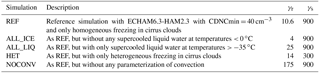
In this paper, we compare results from the release version of ECHAM6-HAM2 with CDNCmin = 40 cm⁻³ (simulation REF) and the sensitivity simulations discussed below with observations. To address the impact of SLF on ECS in ECHAM6-HAM2, we conducted one simulation with no supercooled liquid water below 0 ^∘C (simulation ALL_ICE) and one simulation with no ice formation at temperatures > −35 ^∘C (simulation ALL_LIQ), similar to what has been done in Tan et al. (2016) and Lohmann (2002). The simulation ALL_ICE is set up such that all cloud droplets that are advected to colder temperatures are forced to freeze instantaneously and all the detrained cloud condensate is in the form of ice at temperatures < 0 ^∘C. The simulation ALL_LIQ is set up such that heterogeneous freezing is turned off in the temperature range between 0 and −35 ^∘C and detrainment of ice crystals from convective clouds is restricted to temperatures below −35 ^∘C. Ice crystals sedimenting from colder into warmer cloud layers melt at −35 ^∘C. The number of cloud droplets which freeze at temperatures below −35 ^∘C had to be reduced by a factor of 100 in order to keep the ice crystal number concentration realistic in simulation ALL_LIQ and to reduce tuning to a minimum.

In this paper we go beyond the study by Tan et al. (2016) and also test the impact of other aspects of clouds on ECS, such as the type of nucleation in cirrus. There are discussions if cirrus clouds are mainly formed by homogeneous nucleation as we assume in our reference simulation or are nucleated heterogeneously (Cziczo et al., 2013; Spichtinger and Krämer, 2012; Kärcher, 2017). We investigate the impact of homogeneous vs. heterogeneous freezing in cirrus clouds by performing one simulation in which all cirrus clouds form heterogeneously (simulation HET) instead of homogeneous nucleation in simulation REF. Heterogeneously nucleated cirrus clouds are optically thinner (Lohmann, 2008). Thus, with this simulation we aim to address the impact of cirrus on ECS that so far remains uncertain (Boucher et al., 2013).

Last but not least we investigate the impact of parameterized convection on ECS by performing a simulation in which we completely switched off convection (simulation NOCONV) as in Webb et al. (2015). This is normally performed only in simulations run at horizontal resolutions of less than 10 km, at which the vertical motions associated with deep convection start to be resolved. While our horizontal resolution is much coarser and thus a convective parameterization is needed, there are some inconsistencies in terms of microphysics between convective and stratiform clouds. Therefore we evaluate how the cloud fields, the climate in general, and ECS are simulated if only large-scale clouds are allowed to form.

All simulations were performed in T63 spectral resolution, which corresponds to 1.875^∘ × 1.875^∘ and 31 vertical layers with a top at 10 hPa. The present-day atmosphere-only simulations were run over 25 years, after a 3-month spin-up with fixed sea surface temperatures (SSTs) and sea-ice cover (averaged over the atmosphere model intercomparison project (AMIP) climatology for the years 2000–2015). To calculate ECS, ECHAM6-HAM2 has been coupled to a MLO of 50 m depth. The deep ocean heat flux is computed from the atmosphere-only simulations. Because the deep ocean heat flux adjusts to the different set-ups, we computed it individually for each of the five different set-ups used in this study. These simulations were spun up for 25 years after which the simulations were in equilibrium. We then ran them for another 25 years, over which the results were averaged.

The sensitivity studies conducted for our studies are summarized in Table 1. For the calculation of ECS, all simulations need to be in radiative equilibrium at the TOA. This might require retuning. To keep the different simulations as comparable as possible, we only adjusted two parameters inside the two-moment cloud microphysics scheme. γ_r speeds up the autoconversion rate of cloud droplets to grow to raindrops by collision–coalescence and accounts for the missing sub-grid-scale variability in cloud water and CDNC (Wood, 2002). γ_s is the corresponding process in the ice phase, which enhances the aggregation of ice crystals to form snow flakes (Lohmann and Ferrachat, 2010). The values of these two parameters are also included in Table 1. In addition to the changes in the tuning parameters, we needed to decrease the time step from 7.5 to 5 min in simulation NOCONV because of numerical stability.

Table 1Set-up of the simulations together with the two tuning parameters that differ among the simulations.

Download Print Version | Download XLSX

All of the simulations listed in Table 1 were run in three different set-ups: (i) atmosphere-only simulations with prescribed SST and sea ice cover using the AMIP 2000–2015 climatology with present-day aerosol emissions and greenhouse gas concentrations for comparison with observations, (ii) atmosphere–MLO simulations at 1×CO₂ concentrations with preindustrial aerosol emissions and preindustrial levels of the other greenhouse gas, and (iii) atmosphere–MLO simulations at 2×CO₂ concentrations, keeping everything else as in (ii). For simulations (iii) the CO₂ concentration was doubled before the 25-year spin-up period.

An overview of the annual, global mean state of the climate in the different simulations is given in Table 2 together with observations, where available. The observations of global liquid water path (LWP) range between 30 and 90 g m⁻² (Stubenrauch et al., 2013; Platnick et al., 2015, 2017; Stengel et al., 2017a; Poulsen et al., 2017). Elsaesser et al. (2018) restricted the LWP retrievals to ocean regions (LWP_oc) and estimated LWP_oc from a combination of the SSM/I, TMI, AMSR-E, WindSat, SSMIS, AMSR-2, and GMI satellite data (MAC-LWP) as 81.4 g m⁻². Limiting the other retrievals to ocean regions yields a global LWP_oc of 42.9 g m⁻² from MODIS (Platnick et al., 2015, 2017), 43.9 g m⁻² from ATSR-2-AATSR (Stengel et al., 2017a; Poulsen et al., 2017), and 41 g m⁻² from AVHRR-PM (Stengel et al., 2017b), illustrating the huge uncertainty of estimating LWP_oc. All simulations except for ALL_LIQ fall within this range. In simulation ALL_LIQ, LWP_oc amounts to 110 g m⁻² because no ice is formed at temperatures > −35 ^∘C.

The annual zonal mean LWP and ice water path (IWP) from all simulations as well as from satellite observations of LWP from multiple satellite sensors (Elsaesser et al., 2018), the MODIS satellite (Platnick et al., 2015, 2017), and the ATSR-2-AATSR satellites (Stengel et al., 2017a; Poulsen et al., 2017) and IWP from CALIPSO/CloudSat (Li et al., 2012) are shown in Fig. 1. Because the MAC-LWP observations are only available over oceans, we limit the comparison of LWP to ocean regions. Both retrievals from visible–near-infrared sensors and microwave sensors have biases in retrieving LWP (Seethala and Horvath, 2010; Lebsock and Su, 2014). Lebsock and Su (2014) mentioned four biases in LWP retrievals for MODIS (visible–near-infrared sensor) and AMSR-E (microwave sensor): a bias at large solar zenith angles (MODIS), missing pixels of low-lying clouds that are not detected (MODIS), LWP retrievals in cloud-free scenes (AMSR-E), and the partitioning of the microwave signal between cloud and precipitation signals (AMSR-E). The LWP bias of microwave-sensor-based products in clear-sky scenes has been recently corrected by Elsaesser et al. (2018). The LWP estimates of microwave retrieval products are most reliable in regions where LWP is much larger than the rainwater path (RWP). Thus, Elsaesser et al. (2018) recommend restricting the LWP satellite data to regions in which LWP∕(LWP + RWP) > 0.8. This LWP_{oc,low_pr} covers areas dominated by stratocumulus, trade wind cumulus regions in the subtropics, the Southern Ocean, high latitudes in the Northern Hemisphere, and parts of the north Atlantic and north Pacific. LWP_{oc,low_pr} from MAC-LWP should thus have the smallest retrieval biases. Therefore we use it to evaluate the model LWP as shown in Fig. 1.

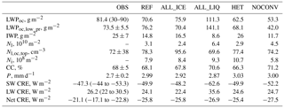
Table 2Global annual mean of oceanic LWP_oc; LWP_{oc,low_pr}; IWP; vertically integrated global cloud droplet (N_l); CDNC at cloud top over oceans ($N_{\mathrm{l},\mathrm{oc},\mathrm{top}}$); ice crystal number concentration (N_i); total cloud cover (CC); precipitation rate (P); shortwave (SW), longwave (LW), and net cloud radiative effect (CRE) from observations; and 20-year atmosphere-only present-day model simulations with prescribed SST as described in Table 1 for 2003–2012. The satellite observations of LWP_oc are taken from Platnick et al. (2015, 2017), Stengel et al. (2017a), Poulsen et al. (2017), and Elsaesser et al. (2018); of LWP_{oc,low_pr} from Elsaesser et al. (2018); of IWP from the CloudSat/CALIPSO satellites (Li et al., 2012); of $N_{\mathrm{l},\mathrm{oc},\mathrm{top}}$ from Bennartz and Rausch (2017) of total cloud cover from Stubenrauch et al. (2013) and Matus and L'Ecuyer (2017); of precipitation rate from the GPCP version 2.3 data set (Adler et al., 2003, 2012). The CRE satellite data are averaged over the period 2001–2011 from the Clouds and the Earth's Radiant Energy System Energy Balanced and Filled Ed2.6r data set (Boucher et al., 2013) and are described in Loeb et al. (2009, 2018). For the uncertainty range of the SW CRE data from CloudSat and CALIPSO are also considered (Matus and L'Ecuyer, 2017) and for LW CRE data from the TOVS satellite are also considered (Susskind et al., 1997). See legend of Fig. 1 for details of the observations.

Download Print Version | Download XLSX

The new multi-satellite observations of LWP_oc by Elsaesser et al. (2018), averaged over the years 1988–2016, show a maximum LWP in the tropics and, on average, their estimate is twice as high as the retrievals from MODIS and ATSR-2-AATSR both for the years 2003–2012. LWP_oc from MODIS and ATSR-2-AATSR, conversely, increases towards the poles and only a weak secondary maximum is indicated near the Equator. All observations show high values of LWP_oc in the storm tracks in both hemispheres, but the exact location varies among the different observations. The most noticeable difference between LWP_oc and LWP_{oc,low_pr} is the absence of data in the intertropical convergence zone (ITCZ). In fact, the agreement of simulations REF and HET in terms of the zonal mean structure of LWP_{oc,low_pr} with observations is very good everywhere and better than with LWP_oc. LWP_{oc,low_pr} is too low at high latitudes in simulation ALL_ICE and the maxima in the extratropics are overestimated in simulation ALL_LIQ. LWP_{oc,low_pr} is underestimated everywhere in simulation NOCONV because of the large speedup of the autoconversion rate required to reach radiative equilibrium at the TOA in this set-up.

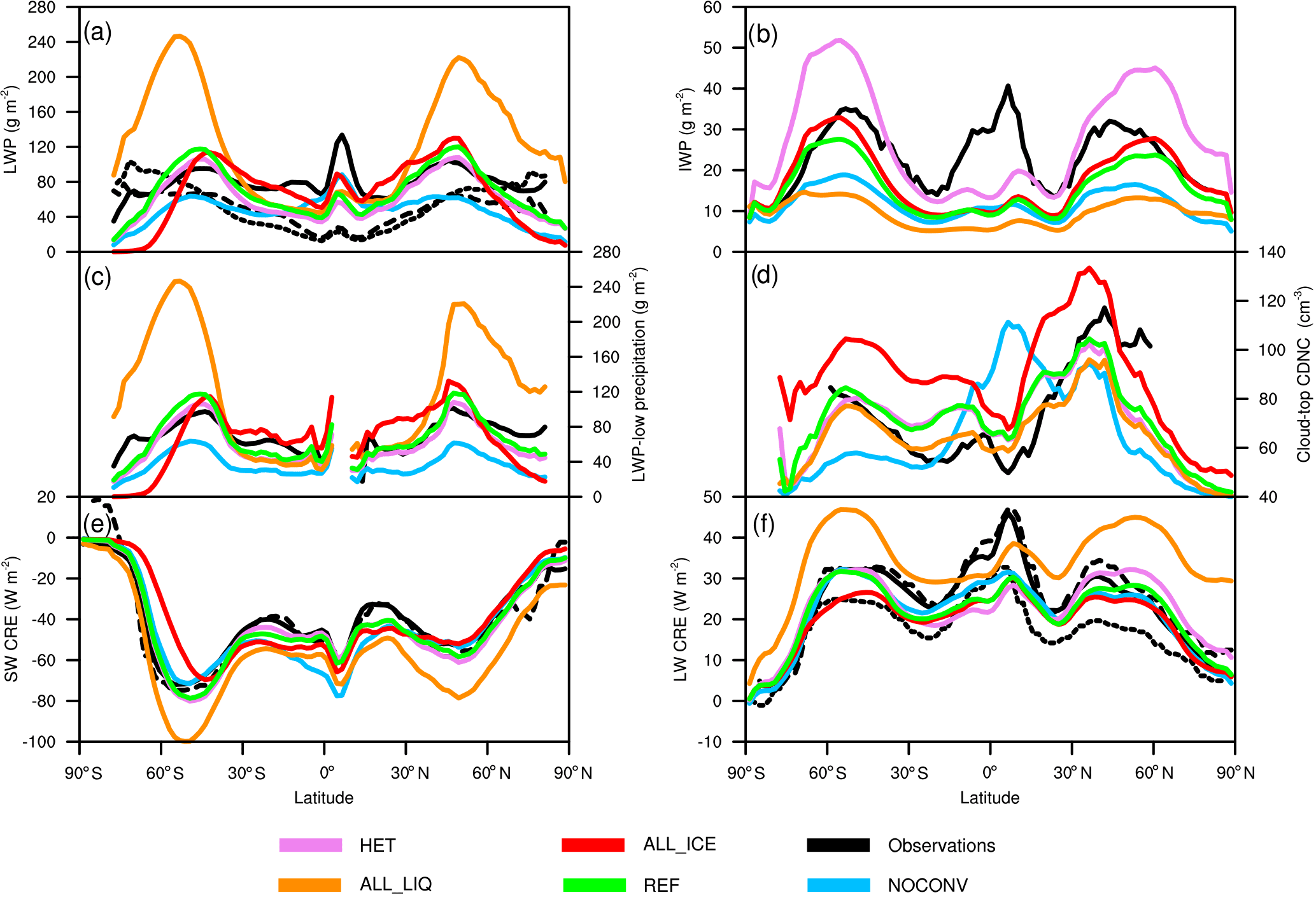
Figure 1Annual zonal mean LWP_oc (a), IWP (b), LWP_{oc,low_pr} (c), cloud-top CDNC of clouds between 268 and 300 K (d), SW CRE (e), and LW CRE (f) from the atmosphere-only present-day simulations for the years 2003–2012 as described in Table 1 and observations of LWP from multiple satellite sensors for the years 1988–2016 by Elsaesser et al. (2018) (solid line), from MODIS-AQUA collection 6.1 for the years 2003–2012 (Platnick et al., 2015, 2017) (dotted line), from ATSR-2-AATSR for the years 2003–2012 (Stengel et al., 2017a) (dashed line), CloudSat + CALIPSO satellite observations of IWP for the years 2006–2010 from Li et al. (2012), low-precipitating oceanic LWP from Elsaesser et al. (2018) for the years 2003–2012, oceanic cloud-top CDNC for the years 2003–2015 from Bennartz and Rausch (2017), SW and LW CRE. The solid SW and LW CRE lines are from CERES 2003–2012 (Loeb et al., 2009, 2018), the dashed ones from ERBE for the years 1985–1989, and the dotted ones for LW CRE from TOVS satellite data for the years 1985–1993 (Susskind et al., 1997).

Download

The cloud-top CDNC for oceanic clouds ($N_{\mathrm{l},\mathrm{oc},\mathrm{top}}$) with temperatures between 268 and 300 K has been obtained from satellite data (Bennartz and Rausch, 2017) for the years 2003–2015. From the model simulations, oceanic cloud-top CDNCs were used for temperatures > 273.2 K. $N_{\mathrm{l},\mathrm{oc},\mathrm{top}}$ is less zonally symmetric than LWP as a result of the higher emissions in the Northern Hemisphere. $N_{\mathrm{l},\mathrm{oc},\mathrm{top}}$ reaches values of > 100 cm⁻³ between 30 and 60^∘ N in the observations (Fig. 1). All model simulations fail to produce such high values north of 40^∘ N, probably because of an insufficient transport of aerosol particles to the Arctic (Bourgeois and Bey, 2011), missing nitrate aerosols, and underestimation of particulate organic aerosols (Zhang et al., 2012), all of which contribute to underestimating the concentration of cloud condensation nuclei. $N_{\mathrm{l},\mathrm{oc},\mathrm{top}}$ is well simulated south of 30^∘ N, especially in simulation ALL_LIQ. $N_{\mathrm{l},\mathrm{oc},\mathrm{top}}$ is highest in simulation ALL_ICE (Table 2) and overestimated with respect to the observations. This is caused by the lower speedup of the autoconversion rate in simulation ALL_ICE (Table 1), which reduces the sink of cloud droplets in this simulation and causes higher CDNC at all altitudes compared to simulation REF (not shown).

The zonal distribution of $N_{\mathrm{l},\mathrm{oc},\mathrm{top}}$ in simulation NOCONV differs from the other simulations. It peaks near the Equator because the clouds here cannot form by convection and instead the stratiform cloud scheme needs to take over. As the rain formation depends on CDNC only in the stratiform cloud microphysics scheme but not in the convective one, warm rain is less efficiently formed in the tropics in the stratiform scheme, causing a buildup of cloud droplets in simulation NOCONV as portrayed in Fig. 1. The CDNC peak in the tropics in simulation NOCONV deviates strongly from observations, as do the lower-than-observed values in the extratropics.

ECHAM6-HAM2 in general has problems simulating IWP values in the observed range. This deficiency can largely be attributed to an underestimation in the ice crystal size in simulation REF at least for clouds with a COD < 3 (Gasparini et al., 2018). The only simulation in which IWP in the global mean agrees with the observations is simulation HET (Table 2) because the heterogeneous nucleation is limited by the number concentration of dust aerosols. The dust number concentration is smaller than the number concentration of soluble aerosols that can freeze homogeneously and freezing commences at a lower relative humidity and a higher temperature in simulation HET. Because of the limited number concentration of dust aerosols and the faster depositional growth at higher temperatures, the heterogeneously nucleated ice crystals are larger than the ones nucleated homogeneously. Because of this, they sediment and aggregate more rapidly, causing simulation HET to be initially out of radiative balance. Here retuning was necessary to slow down the rate of aggregation and at the same time speed up the rate of autoconversion. This resulted in one of the lowest LWPs of all simulations and the highest IWPs with the highest ice crystal number concentration.

The IWP peak in the tropics in Fig. 1 is related to liquid-origin cirrus clouds (Wernli et al., 2016; Kraemer et al., 2016; Gasparini et al., 2018) forming the anvils from deep convection in the ITCZ as well as in the warm conveyor belt in the storm tracks. The peak in the ITCZ is not captured in any of the model simulations, suggesting that the model severely underestimates the detrained cloud ice in deep convective clouds. Cloud ice in the extratropics is underestimated in all simulations but simulations HET and ALL_ICE. IWP is largest in simulation HET due to retuning as discussed above. Its zonal distribution shows that the underestimation of IWP in the tropics is compensated for by an overestimation in the extratropics. Simulation ALL_ICE best matches the magnitude of IWP in the extratropics but shifts the peaks slightly polewards of the observations.

The total cloud cover in ECHAM6-HAM2 is that of large-scale clouds because convective clouds are considered to be short lived and to decay within one model time step except for the detrained condensate in the anvils that is taken as a source for the stratiform cloud scheme. The global mean total cloud cover does not vary much among the different simulations and it falls within the observed range of 68 ±5  % (Stubenrauch et al., 2013) in all simulations. It is second-largest in simulation ALL_LIQ because of its large LWP. It is highest in simulation NOCONV because here all clouds are large scale and contribute to the cloud cover.

The observed precipitation rate from GPCP of 2.7 mm d⁻¹ (Adler et al., 2003) averaged over 1981–2010 is overestimated by 6–13 % in all simulations, a feature that ECHAM6-HAM2 shares with its host model ECHAM6 (Stevens et al., 2013). As discussed in Stevens et al. (2013), GPCP seems to underreport precipitation, and higher precipitation rates are more consistent with the best observational estimates of the surface energy budget (Stephens et al., 2012).

The cloud radiative effect (CRE) is the difference between the all-sky radiation at the TOA and the clear-sky radiation. The shortwave (SW) CRE amounts to −47.3 W m⁻² with a range from −46 to −53.3 W m⁻² in the satellite data (Loeb et al., 2009, 2018; Zelinka et al., 2017). In all simulations, except ALL_LIQ, SW CRE amounts to about −50 W m⁻², which lies within the observed range. SW CRE is most negative and outside the observational range in simulation ALL_LIQ because of its high LWP and total cloud cover (see also Fig. 1). Conversely, it is least negative in simulation ALL_ICE, in which LWP is rather small and hence τ is smallest. Here SW CRE is severely underestimated south of 40^∘ S due to the lack of supercooled liquid water. While too much absorption of shortwave radiation over the Southern Ocean has been a problem in the many GCMs because of insufficient supercooled liquid water (e.g., Williams et al., 2013; Bodas-Salcedo et al., 2014; Kay et al., 2016), in our model this problem only arises in the extreme simulation ALL_ICE.

LW CRE amounts to 26.2 W m⁻² with a range from 22 to 30.5 W m⁻² in the satellite data (Loeb et al., 2009, 2018; Susskind et al., 1997; Zelinka et al., 2017). As for SW CRE, all simulations but ALL_LIQ calculate LW CRE to be about 24–25 W m⁻² in good agreement with observations. Again LW CRE is smallest in simulation ALL_ICE and highest and outside the observational range in simulation ALL_LIQ (see also Fig. 1). Due to the severe underestimation of cloud ice in the tropics in all simulations, LW CRE is systematically underestimated in the tropics. The exception is simulation ALL_LIQ in which the underestimation in tropical cloud ice is compensated for by the thickest high level clouds (Fig. 2).

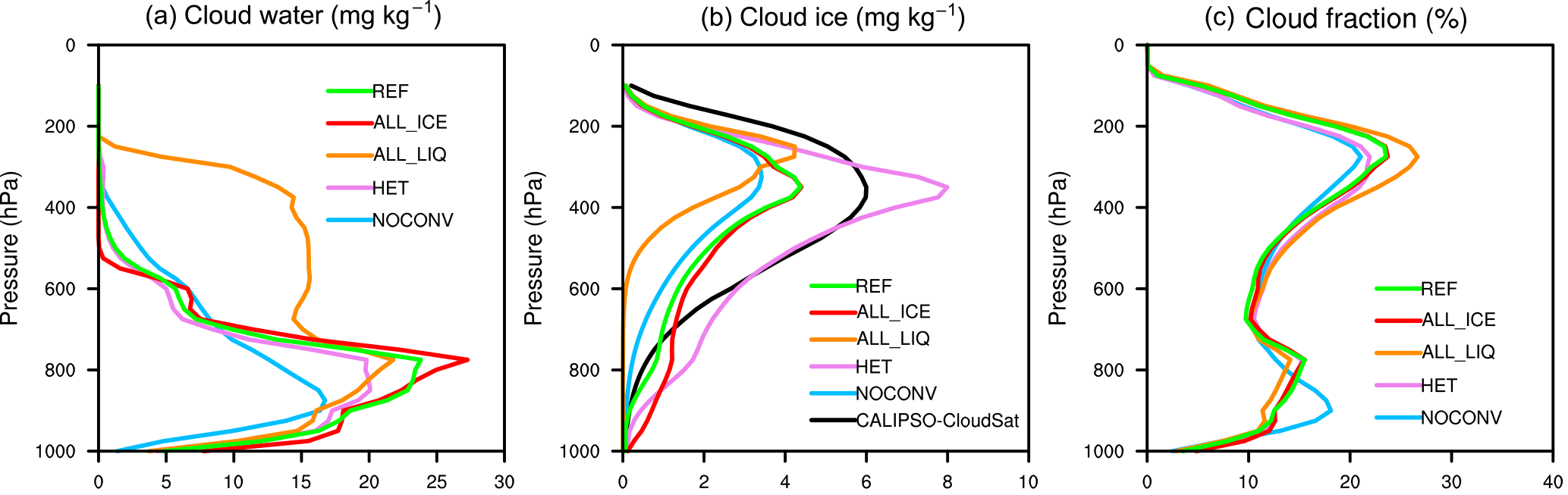
Figure 2Annual global mean cloud liquid water content (a), ice water content (b) in milligrams per kilogram, and cloud cover (c) in percent as a function of pressure in hectopascals from the various sensitivity atmosphere-only present-day simulations for the years 2003–2012 described in Table 1 and observations of the ice water content from CALIPSO-CloudSat for the years 2006–2010 by Li et al. (2012).

Download

The global mean observed net CRE ranges between −17.1 and −22.8 W m⁻². Here all simulations are more negative than observed, i.e., they overestimate the net negative radiative effect of clouds.

The vertical distribution of the globally and annually averaged cloud liquid water and cloud ice is shown in Fig. 2. Cloud liquid water has its maximum at around 800 hPa associated with low clouds where it varies between 20 and 30 mg kg⁻¹ in the different simulations. It is lowest in simulation NOCONV because of the drastically enhanced autoconversion rate (Table 1). Cloud liquid water decreases to zero at around 400 hPa except in simulation ALL_LIQ in which ice formation is limited to temperatures < −35 ^∘C. Unfortunately no observational data of the vertical distribution of cloud liquid water are available.

The vertical distribution of cloud ice has been derived from CALIPSO/CloudSat (Li et al., 2012). It peaks at 400 hPa with 6 mg kg⁻¹ and becomes negligible at altitudes above 100 hPa and below 900 hPa (Fig. 2). Here the differences among the sensitivity experiments are more pronounced. In simulations REF and NOCONV the shape of the distribution looks similar to the observed distribution, but the peak value is underestimated by 30–50 % and in simulation REF a secondary maximum is present at around 780 hPa. This peak is related to cloud ice over the Southern Ocean and Antarctica (not shown). In simulation ALL_LIQ, in which the global annual mean IWP is smallest due to suppressed ice formation in mixed-phase clouds, cloud ice peaks at 250 hPa and drops to zero at 600 hPa. This simulation differs most from the observations. It also has the lowest cloud cover in the lower troposphere and the highest cloud fraction between 200 and 400 hPa (Fig. 2). Conversely, simulation NOCONV has the highest coverage of low-level clouds and the smallest coverage of cirrus clouds.

In simulation ALL_ICE the comparison of cloud ice with observations is also less favorable compared to simulation REF because more cloud ice than observed is simulated in the lower atmosphere while the underestimation of cloud ice at higher altitudes has not noticeably improved. The overall best agreement with observations is seen in simulation HET. This is the only simulation in which the global annual mean IWP lies within the observational uncertainty (Table 2). However, the peak in cloud ice at 400 hPa is 25 % too large and too narrow. Although the freezing mechanism was only changed for cirrus clouds, the overall higher amount of cloud ice extends to lower altitudes, causing an overestimation in cloud ice between 600 and 900 hPa. This is mainly a result of the reduced speedup of the aggregation rate that also affects cloud ice in mixed-phase clouds.

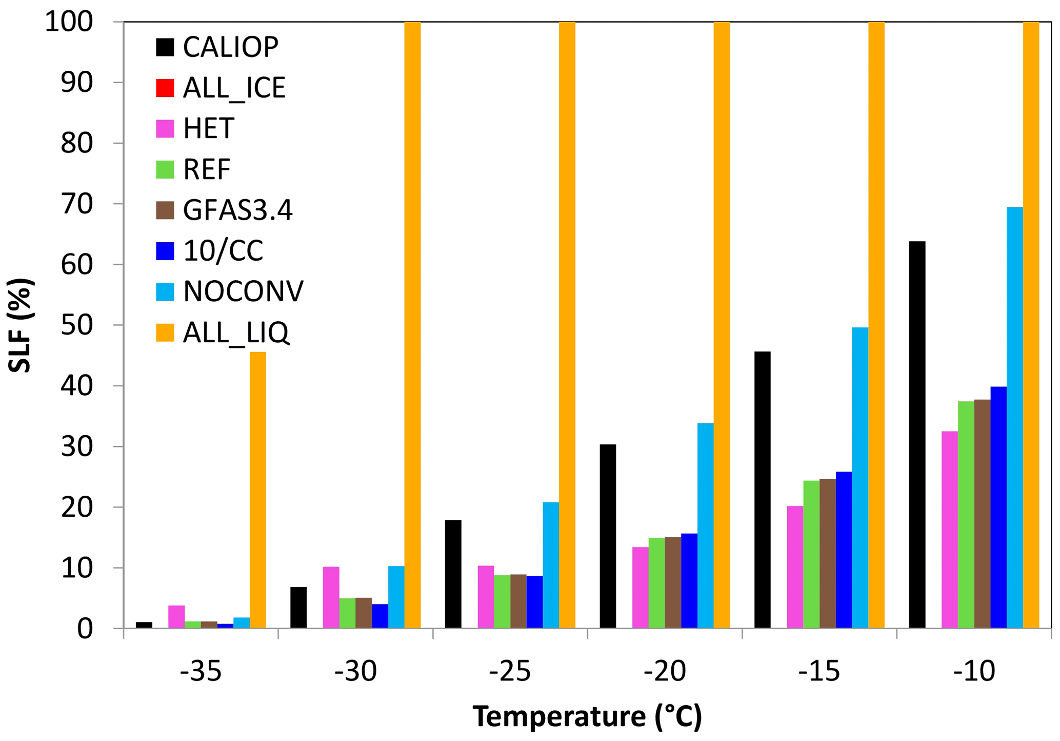
SLF has been obtained from the CALIOP satellite and has been compared to an earlier version of ECHAM6-HAM2 (Komurcu et al., 2014). At that time ECHAM6-HAM2 seriously underestimated SLF. This can partly be explained by differences in the definition of SLF in the satellite data and in the model. In addition, some of the model improvements mentioned above were added after the study by Komurcu et al. (2014). As the lidar signal becomes attenuated at COD > 3, the CALIOP satellite data are only representative for all cloud tops not overlaid by clouds with COD > 3. SLF of the model data is diagnosed similarly to CALIOP starting from the highest cloud layers as long as the cumulative COD of these cloud layers is less than or equal to 3. As shown in Fig. 3, ECHAM6-HAM2 still underestimates SLF but on average simulates SLFs twice as high as presented in Komurcu et al. (2014). At −10 ^∘C SLF amounts to 63 % in CALIOP but only 37 % in simulation REF. The difference between the observed and simulated SLF decreases at colder temperatures because of the general decrease in SLF with decreasing temperature.

SLF from all ECHAM simulations is significantly underestimated except for simulations ALL_LIQ and NOCONV. Simulation NOCONV actually matches the observed SLF rather well, mainly because supercooled liquid water exists at higher altitudes than in simulation REF (Fig. 2). This points to a potential deficiency as to how we handle detrainment from convective clouds or convection itself. In simulation REF we assume that if we are in the Wegener–Bergeron–Findeisen (WBF) regime, following the definition of Korolev (2007) as described in Lohmann and Hoose (2009), and cloud ice is already present, the detrained condensate will be in the form of ice. It is only detrained as supercooled liquid water if the vertical velocity is sufficiently high to exceed saturation with respect to liquid water. This assumption seems to cause a too efficient WBF process, thus depleting the supercooled liquid water too rapidly. We will rethink our approach in the future.

The control simulation in CESM from Tan et al. (2016) simulates a SLF of only 20 % at −10 ^∘C. Based on their hypothesis that an underestimation in SLF translates into an underestimation in ECS, a smaller underestimation of SLF in simulation REF should lead to a smaller underestimation of ECS in ECHAM6-HAM2. Based on the simulated SLFs, we expect ECS to be lowest in simulation ALL_ICE and to successively increase in simulations HET, REF, NOCONV, and ALL_LIQ.

Figure 3Frequency of occurrence of SLF in percent for clouds with COD < 3 in different temperature bins from CALIOP observations for the years 2006–2010 and the various sensitivity simulations from the atmosphere-only present-day simulations for the years 2003–2012 described in Table 1.

Download

In a warmer climate, the saturation-specific humidity increases by 7 % ^∘C⁻¹ of temperature increase according to the Clausius–Clapeyron equation. Because the relative humidity has been found to remain rather constant (Soden et al., 2002), this causes an increase in the specific humidity and speeds up the hydrological cycle leading to higher liquid water contents in clouds and higher precipitation rates.

ECS from all our sensitivity simulations is shown in Table 3. It ranges between 1.8 and 2.6 K and with that lies on the lower side of the range of ECS estimated in the last IPCC report (Collins et al., 2013; Flato et al., 2013) and from CMIP5 models (Forster et al., 2013). Similar to Tan et al. (2016), ECS increases by ∼ 30 % when increasing SLF from almost zero to one (simulations ALL_ICE and ALL_LIQ in this paper vs. Low-SLF and High-SLF in Tan et al., 2016). Contrary to their large increase in ECS from their reference simulation to simulation High-SLF, ECS does not change among simulations REF, NOCONV, and ALL_LIQ but remains at ∼ 2.5–2.6 K despite the increase in SLF at −10 ^∘C from ∼ 30 % in HET and ∼ 40 % in REF to ∼ 70 % in NOCONV and 100 % in ALL_LIQ, i.e., only ECS in simulation ALL_ICE is noticeably different. This suggests that ECHAM6-HAM2 is more sensitive at low SLF. These results seem to support the hypothesis that an increase in ECS is only sensitive to SLF if too little shortwave radiation is reflected back to space from mixed-phase midlatitude clouds, i.e., when they are composed of ice instead of liquid water. This has also been suggested by Frey and Kay (2017), who modified CAM5 to detrain more liquid water at colder temperatures in shallow convective clouds, which occur in the cold sector of midlatitude cyclones, for example. It is important that these mixed-phase clouds are not shielded by ice clouds in order for a change in their cloud phase to affect ECS (Bodas-Salcedo, 2018). Since in ECHAM6-HAM2 this shortwave bias is most pronounced in simulation ALL_ICE, this is the only simulation with a distinctively lower ECS. In the reference version of CAM5, too much shortwave radiation is absorbed over the Southern Ocean in their present-day climate (Kay et al., 2016), which explains why ECS is also sensitive to an increase in SLF in this model (Tan et al., 2016). In addition, Tan et al. (2016) did not use a MLO, but a fully coupled dynamic ocean, which could impact the comparison with our results because different methods can lead to differing ECS estimates (Frey et al., 2017).

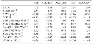
Table 3Global annual mean changes of surface temperature (ΔT_s), liquid water path (ΔLWP), ice water path (ΔIWP), vertically integrated cloud droplet (ΔN_l) and ice crystal number concentration (ΔN_i), total cloud cover (ΔCC), SW CRE (ΔSW CRE), LW CRE (ΔLW CRE), and net CRE from the radiative kernel (RK) method and as normally diagnosed in equilibrium after a CO₂ doubling averaged over the years 26 to 50 of the coupled atmosphere – MLO model simulations as well as the net clear-sky feedback parameter λ^cs diagnosed according to Block and Mauritsen (2013). The individual simulations are described in Table 1. Different from Table 2, here the changes in LWP are global and not limited to ocean regions.

Download Print Version | Download XLSX

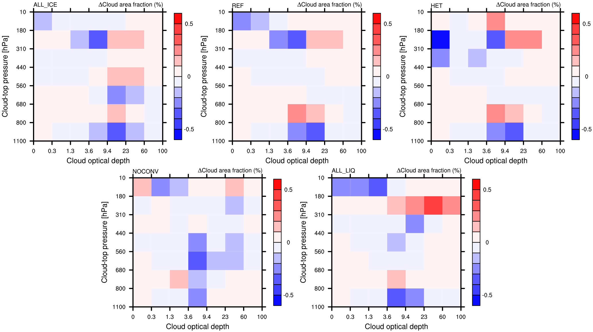
In order to prove our hypothesis for the different relationship between SLF and ECS in ECHAM6-HAM2, we evaluate the changes in cloud fraction as a function of cloud-top pressure and COD between the 2×CO₂ and 1×CO₂ climates. Because mixed-phase clouds are more prevalent in midlatitudes and high latitudes than in the tropics and subtropics (Matus and L'Ecuyer, 2017), we expected the largest differences there. The histograms in Figs. 4 and 5 are taken polewards of 40^∘ latitude in both hemispheres. They are taken from a satellite perspective, by using the COSP-ISCCP simulator (Bodas-Salcedo et al., 2011). This means that the cloud-top pressure refers to the highest cloud in each single sub-column used by the simulator. Sub-columns are used in the simulator to account for sub-grid-scale variability in the cloud (top) distribution. From Fig. 4 we see that only in simulation ALL_ICE is there a large abundance of low- and mid-level optically thin extratropical clouds (with τ<1.3) in the present climate. These clouds show a marked decrease accompanied with a marked increase in medium optical depth clouds ($\mathrm{3.6}<\mathit{\tau }<\mathrm{60}$) between 560 and 800 hPa in the 2×CO₂ climate (Fig. 5). These clouds and their changes are absent in all other simulations with a higher SLF (REF, HET, NOCONV, and ALL_LIQ). Only in simulation ALL_ICE are these optically thin ice clouds not shielded by higher clouds prevalent in the present-day climate (not shown) and are converted to low- and mid-level liquid water clouds of medium optical depth in the 2×CO₂ climate.

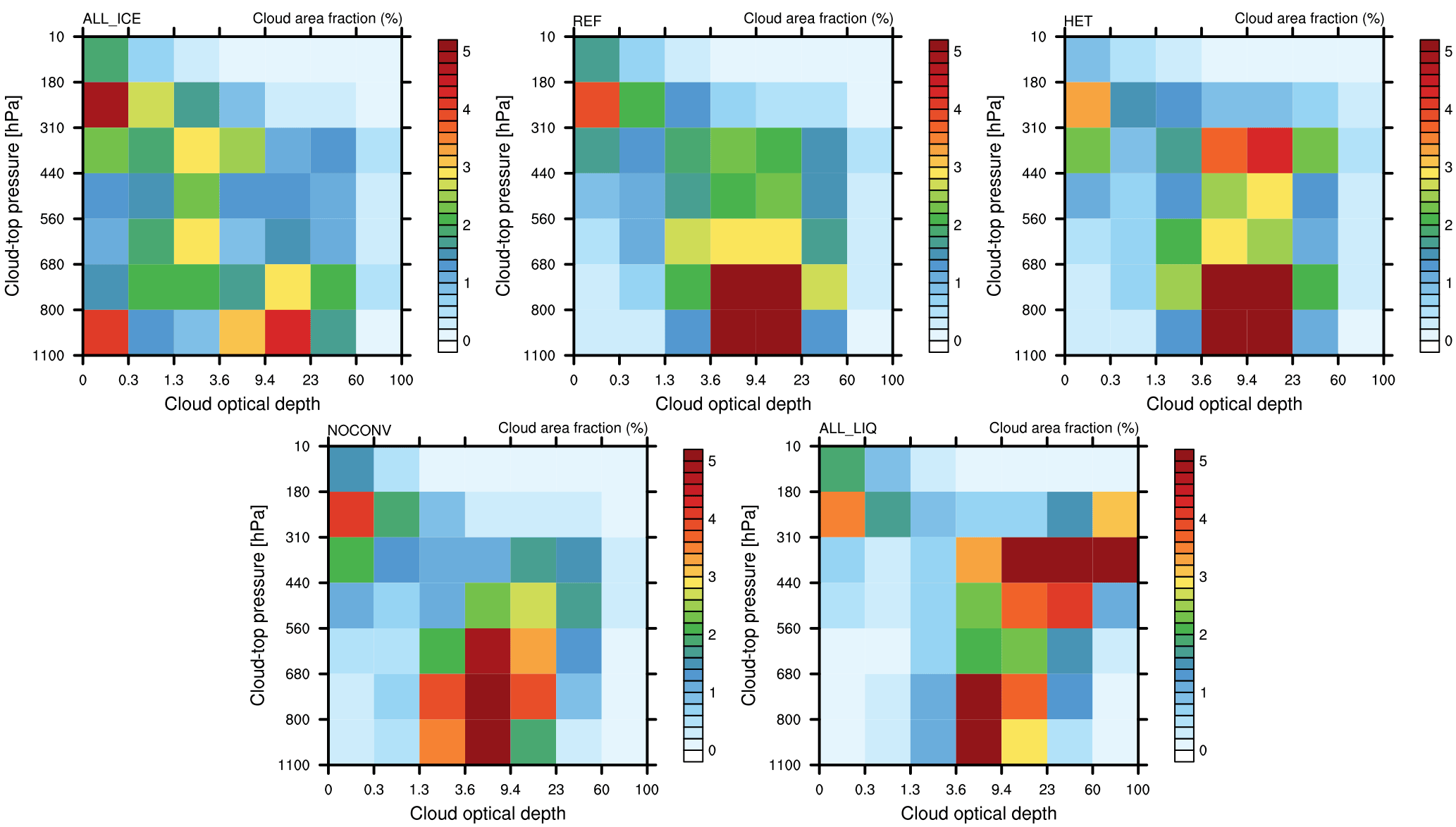
Figure 4Distribution of cloud fraction in the extratropics (> 40^∘ S and N) as a function of cloud optical depth and cloud-top pressure between the 2×CO₂ and the 1×CO₂ climate in simulations ALL_ICE, HET, REF, NOCONV, and ALL_LIQ from the last 25 years of the MLO simulations described in Table 1.

Download

Figure 5Changes in the distribution of cloud fraction in the extratropics (> 40^∘ S and N) as a function of cloud optical depth and cloud-top pressure between the 2×CO₂ and the 1×CO₂ climates in simulations ALL_ICE, HET, REF, NOCONV, and ALL_LIQ from the last 25 years of the MLO simulations described in Table 1.

Download

To estimate the radiative effect of this increase in COD, we calculate the different components of the global cloud feedback parameter λ_c using the radiative kernel decomposition method described in Zelinka et al. (2012a, b). This method decomposes λ_c into feedbacks that are associated with changes in cloud amount λ_amt, cloud-top pressure λ_ctp, and COD λ_τ as shown in Fig. 6 for all simulations. λ_ctp is positive because of the shift of clouds to higher altitudes in the warmer climate (see also Fig. 7) that enhances their LW CRE. At the same time, the total cloud amount decreases in a warmer climate, most noticeable at lower altitudes (Fig. 7). This decrease in low/mid-level clouds reduces the negative net CRE and also constitutes a positive feedback. λ_τ is negative in most simulations and smaller than other cloud feedbacks so that λ_c is positive in most simulations. λ_c is negative (−0.4 W m⁻² K⁻¹) only in simulation ALL_ICE because of its large negative λ_τ. In all other simulations λ_c ranges between 0.3 W m⁻² K⁻¹ and 0.6 W m⁻² K⁻¹. The value of 0.6 W m⁻² K⁻¹ corresponds to the mean of the analyzed GCMs in AR5 (Boucher et al., 2013). The estimates from the other simulations (except ALL_ICE) fall within the 90 % range of the cloud feedback of −0.2 to 0.6 W m⁻² K⁻¹ as assessed in AR5 (Boucher et al., 2013).

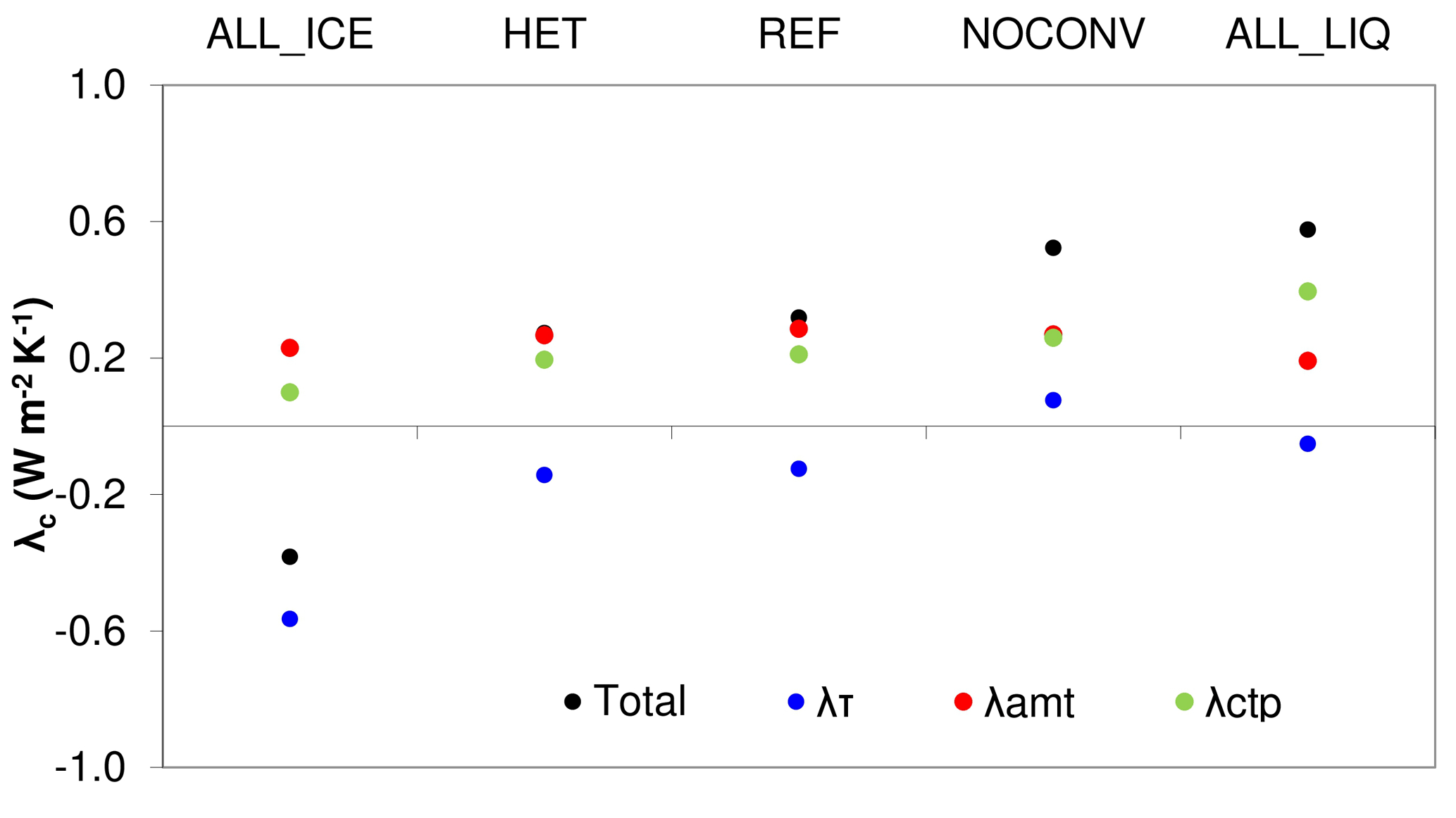
Figure 6Components of the globally averaged cloud feedback parameter λ_c in W m⁻² K⁻¹ for the simulations described in Table 1. λ_τ accounts for changes in cloud optical depth, λ_amt accounts for changes in cloud amount, and λ_ctp accounts for changes in cloud-top pressure.

Download

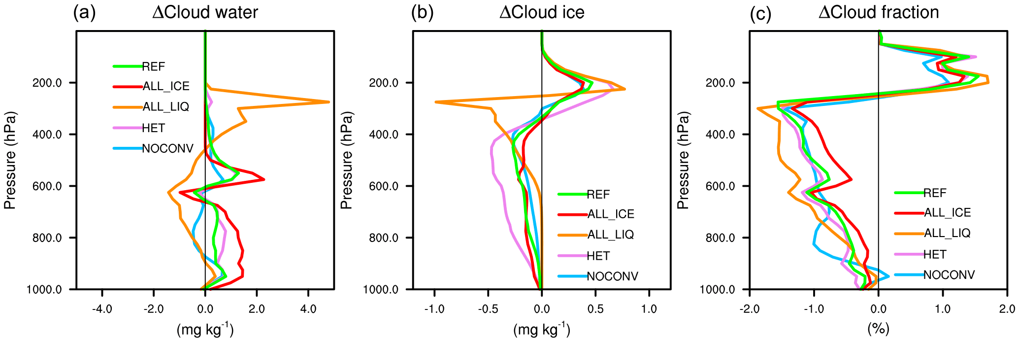
Figure 7Change in the annual global mean cloud liquid water content (LWC, a) and ice water content (IWC, b) in milligrams per kilogram as a function of pressure in hectopascals between the 2×CO₂ and 1×CO₂ climates for the simulations described in Table 1.

Download

The largest differences among the simulations are associated with changes in λ_τ, which varies between −0.6 W m⁻² K⁻¹ in simulation ALL_ICE and 0.1 W m⁻² K⁻¹ in simulation NOCONV. In simulation ALL_ICE, the large negative value of λ_τ can be explained with the largest increase in the LWP of 4.8 g m⁻² (Table 3) due to the phase change from cloud ice to cloud liquid water mainly in low- and mid-level midlatitude clouds (Fig. 5). This causes a negative optical depth feedback in all regions, but most pronounced polewards of 40^∘ (Fig. 8). Note that simulation ALL_ICE is the only simulation in which the overall cloud feedback parameter is dominated by changes in COD. The results of simulation ALL_ICE agree qualitatively with the results from Bodas-Salcedo (2018) for regions with large-scale subsidence in which optically thin ice clouds in the present-day climate are not shielded by higher clouds and hence for which the COD feedback is most important. In all other simulations, the cloud feedback is dominated by changes in cloud amount and cloud-top pressure (Fig. 6).

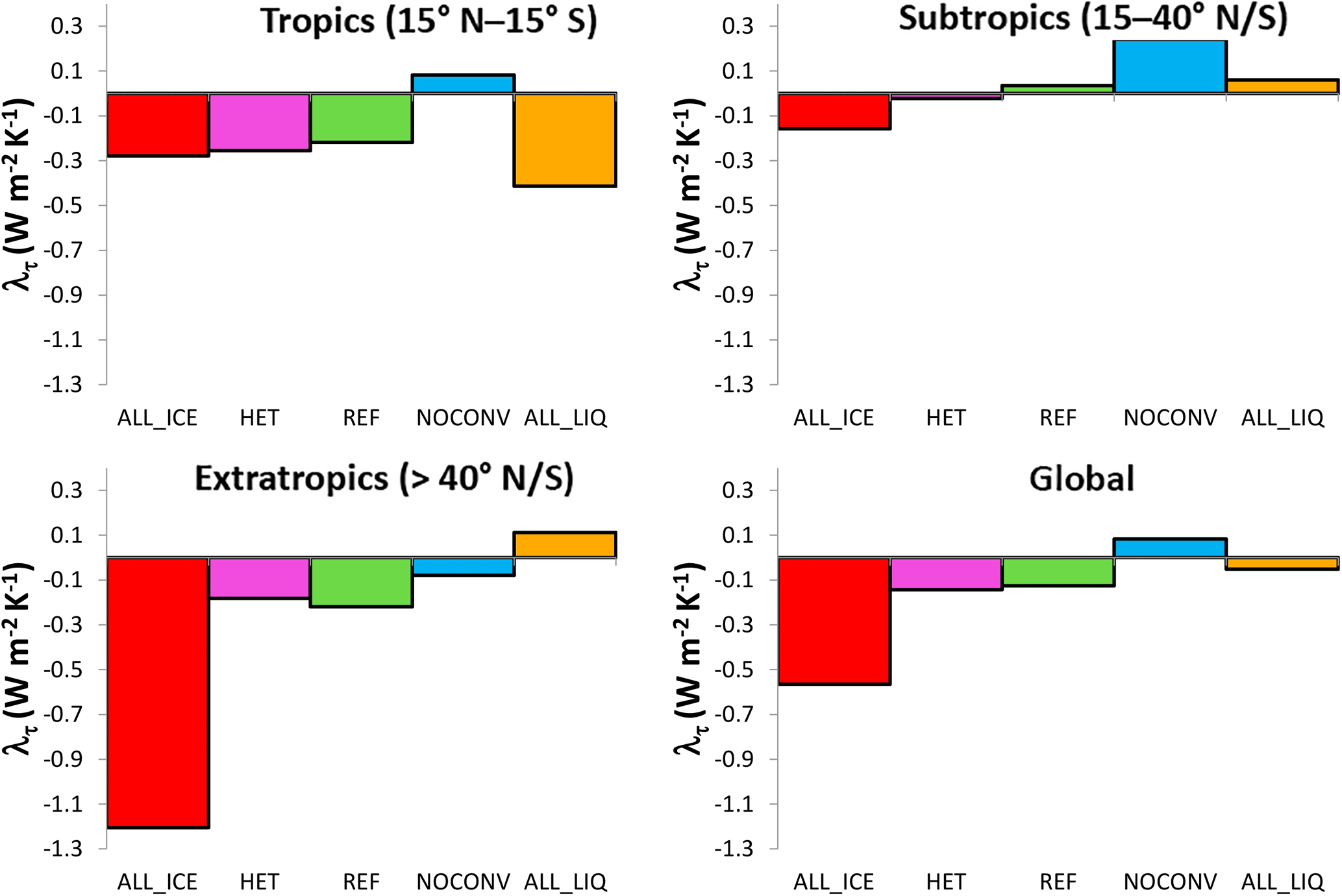
Figure 8Tropical, subtropical, extratropical, and global cloud optical depth feedback parameter λ_τ in W m⁻² K⁻¹ for the sensitivity simulations described in Table 1.

Download

In the other simulations, shown in Fig. 5 for midlatitudes and high latitudes, a rather different picture emerges. Here τ of low clouds hardly changes or decreases as the majority of them are already composed of cloud droplets in the present climate and only a small phase change from ice to liquid occurs due to the doubling of CO₂. In all simulations, except for simulation NOCONV, a negative cloud-phase feedback is also visible in the tropics. This negative feedback arises because some tropical clouds that glaciate at the tops, either due to the presence of ice-nucleating particles in the mixed-phase temperature regime or because their tops extend to altitudes with temperatures < −35 ^∘C in the present climate, will remain supercooled in the warmer climate and hence become optically thicker (Figs. 8 and 9).

Figure 9As Fig. 5 but for the tropics (15^∘ S–15^∘ N).

Download

In the warmer climate, the static stability increases in areas with marine stratus, stratocumulus, and trade wind cumuli in all simulations. This is accompanied by a stronger moisture gradient, which promotes stronger drying by more entrainment (Gettelman and Sherwood, 2016), which in turn causes the marine subtropical clouds to become thinner and their optical depth to decrease. In most simulations this leads to a positive COD feedback in the subtropics as shown in Fig. 8.

The parameterization of convective clouds in ECHAM6-HAM2 assumes that they form and dissipate in one time step. During their lifetime, they can detrain cloud water and ice in the environment. Thus the negative COD feedback in the tropics and midlatitudes indicates that more cloud condensate is detrained in the form of liquid or supercooled liquid water rather than as cloud ice in the warmer climate. Thus, next to the rise of the melting level in the warmer climate, the rise of the homogeneous freezing level is also important for the negative cloud-phase feedback. This is best seen in simulation ALL_LIQ in which no ice exists at mixed-phase temperatures, yet the negative cloud-phase feedback still operates in the tropics (Figs. 8 and 9). In the global mean, this negative cloud-phase feedback is visible in all our simulations as a simultaneous increase in cloud liquid water and decrease in cloud ice in the warmer climate at a given pressure level (Fig. 7). In midlatitudes and the tropics it shows up as an increase in optically thicker clouds and decrease in optically thinner clouds for the same cloud-top pressure (Figs. 5 and 9).

The second most important contributor to the differences in the overall cloud feedback between simulations ALL_ICE and ALL_LIQ is the change in cloud-top pressure (λ_ctp). λ_ctp varies between 0.1 W m⁻² K⁻¹ in simulation ALL_ICE and 0.4 W m⁻² K⁻¹ in simulation ALL_LIQ. The cloud-top pressure feedback is mainly related to cirrus clouds and has been estimated from satellite observations to amount to 0.2 W m⁻² K⁻¹ (Zhou et al., 2014). We obtain a cloud-top pressure feedback of about this value in all other simulations. We also computed the cloud feedbacks separately for low and non-low clouds following the decomposition by Zelinka et al. (2016), which leads to a weaker cloud-top pressure feedback but in general qualitatively similar results for all simulations (not shown).

λ_ctp is largest in simulation ALL_LIQ in which the global mean changes in cloud liquid water and cloud ice are distinctively different from all other simulations (Fig. 7). It is the only simulation in which cloud liquid water decreases throughout the lower and mid-troposphere because here the poleward shift of the storm tracks and the upward shift of convective clouds are least compensated for by changes from cloud ice to cloud liquid water. The changes in simulation ALL_LIQ are accompanied with the largest decrease in cloud cover between 750 and 370 hPa. Cloud liquid water increases between 250 and 400 hPa at the expense of cloud ice in simulation ALL_LIQ. In all other simulations, the concurrent increase in cloud liquid water and decrease in cloud ice occurs at altitudes below 400 hPa. The different vertical structure of cloud liquid water and cloud ice in simulation ALL_LIQ is a consequence of the design of this simulation. Because cloud ice only forms at temperatures below −35 ^∘C, cloud droplets are carried upwards to this temperature, such that the optically thick clouds extend to higher altitudes in the 2×CO₂ climate (see Figs. 5 and 9), causing the largest cloud-top pressure feedback as shown in Fig. 6.

The opposite effect can be seen in simulation ALL_ICE, in which all cloud water is converted to ice already at 0 ^∘C. The increase in cloud liquid water in low and mid-level clouds in the warmer climate is largest in this simulation mainly because of the negative cloud-phase feedback (Fig. 7). This combined with only a modest increase in cloud ice and cloud cover between 250 and 100 hPa (Fig. 7) causes the cloud-top pressure feedback to be smallest in this simulation (Fig. 6).

Simulation NOCONV is the only simulation in which λ_τ is slightly positive. λ_τ is negative in all other simulations in the tropics (Fig. 8) because more cloud condensate is detrained in the form of liquid or supercooled liquid water in the warmer climate. The absence of a convection parameterization and hence detrainment in simulation NOCONV on average leads to a positive tropical λ_τ, i.e., the tropical and subtropical clouds in simulation NOCONV become optically thinner.

To summarize, the negative COD feedback only dominates the overall cloud feedback if the low- and mid-level midlatitude clouds consist of ice in the present climate and change to liquid in the 2×CO₂ climate as in simulation ALL_ICE. However, this does not imply that the overall cloud feedback remains more or less constant in the other simulations. In fact, λ_c almost doubles from simulations REF and HET to simulations NOCONV and ALL_LIQ, caused by the large increase in cloud-top pressure feedback in simulation ALL_LIQ and a positive λ_τ in simulation NOCONV as explained above. This marked increase in the overall cloud feedback from simulations HET and REF to simulations NOCONV and ALL_LIQ is, however, not reflected in an increase in ECS because the net clear-sky feedback parameter, i.e., the sum of the clear-sky Planck, water vapor, lapse rate, and surface albedo feedbacks, is largest in simulation ALL_LIQ followed by simulation NOCONV (Table 3).

We hypothesize that different processes contribute to the rather similar ECS in all simulations but ALL_ICE: in simulation ALL_LIQ, this seems to be caused by the optically thick clouds that tend to cluster in the tropics and become optically thicker there. This is apparent from Fig. 9, in which the upward shift in cirrus clouds with an increase in cirrus optical depth between 180 and 310 hPa is much more pronounced in simulation ALL_LIQ than in simulation REF. In addition, the negative cloud-phase feedback is restricted to ice clouds that formed at altitudes with temperatures < −35 ^∘C in the 1×CO₂ climate that are now liquid clouds (Fig. 7).

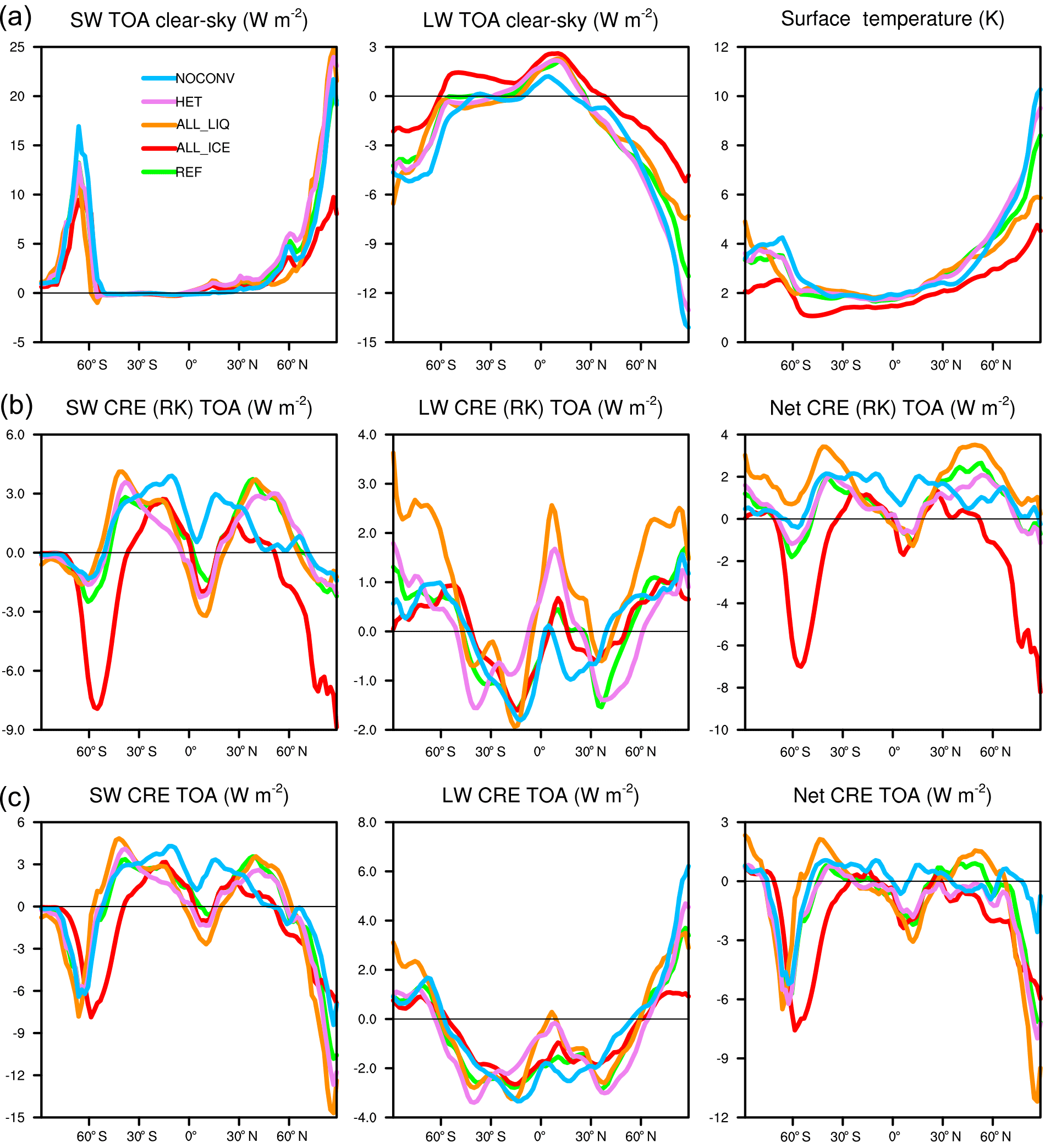
Figure 10Changes in the annual zonal SW and LW net clear-sky radiation in watts per square meter at the top-of-the-atmosphere and surface temperature (K) (a); changes in SW, LW, and net cloud radiative effects between the 2×CO₂ and 1×CO₂ climates calculated based on the radiative kernel method (b) and normally diagnosed (c) for the simulations described in Table 1. Negative values for the change in clear-sky outgoing longwave radiation denote higher values in the 2×CO₂ climate. Please note the different vertical axes.

Download

This increase in optical depth of high clouds causes their SW CRE to be more negative and completely offsets the reduction in LW CRE from the decrease in cloud cover in the tropics in simulation ALL_LIQ (Fig. 10). Such a clustering of convective clouds was found by Lohmann and Roeckner (1995) using the ECHAM4 model when the emissivity of cirrus clouds was set to 1 (black cirrus), i.e., when the infrared optical depth was increased. No convective clustering was seen in the reference simulation in which the cirrus emissivity was calculated as a function of ice water path and in a simulation with transparent cirrus in the infrared. In a warmer climate, convective clouds have been found to cluster further (Bony et al., 2016). The clustering of convective clouds in the warmer climate arises because cloud tops remain at nearly the same temperature in a warmer climate (e.g., Hartmann and Larson, 2002) but are in a more stable environment, which decreases anvil outflow in the upper troposphere and decreases the anvil cloud fraction (Bony et al., 2016). In ECHAM this decrease is most pronounced at altitudes below 250 hPa (Fig. 7) from which more longwave radiation is emitted to space. This leads to an overall negative feedback (e.g., Hartmann and Larson, 2002; Mauritsen and Stevens, 2015) because of the much larger clear-sky area and offsets the positive cloud feedback. In the present-day climate of simulation ALL_LIQ, the least amount of outgoing longwave radiation is emitted to space because the clouds are optically thickest in this simulation. In a warmer climate, these clouds cluster further in the intertropical convergence zone as can be seen from the largest increase in LW CRE as diagnosed from the radiative kernel (RK) method (Fig. 10). Because these clouds are optically thick, this large increase in LW CRE (RK) is overcompensated for by a decrease in SW CRE (RK), causing the net CRE (RK) in the intertropical convergence zone to be as negative in simulation ALL_LIQ as in simulation REF.

The cloud-top pressure feedback in the extratropics that is significantly positive in all simulations but ALL_ICE where it is close to zero (not shown) is overcompensated for by decreases in cloud cover. As shown in Fig. 10, SW CRE and SW CRE (RK) become less negative in the extratropics and dominate over the decrease in LW CRE and LW CRE (RK), causing a positive Δnet CRE at midlatitudes. The generally smaller positive and larger negative changes in net CRE than in net CRE (RK) are caused by compensating changes in non-cloud climate components as described in detail in Shell et al. (2008). In high latitudes, the decrease in surface albedo due to melting of Arctic sea ice causes especially large negative ΔSW CRE and Δnet CRE values polewards of 70^∘ N. In the clear-sky, water vapor and CO₂ absorb more longwave radiation in the warmer climate than in the present day. This decreases the difference between all-sky and clear-sky fluxes and causes the LW CRE to be less positive. Differences in surface temperature operate in opposite ways. While more longwave radiation is emitted to space in the warmer climate (negative Planck feedback), more longwave radiation is also absorbed by clouds and re-emitted to the surface (positive cloud feedback). This clear-sky compensation in the longwave is most pronounced in simulation ALL_LIQ, which is the only simulation in which the global mean ΔLW CRE (RK) is positive (Table 3).

The changes between simulation REF and ALL_LIQ are qualitatively comparable to the ones from Lohmann and Roeckner (1995), for which the difference in climate sensitivity was also rather small between the reference simulation and the black cirrus simulation, both of which also had a positive cloud feedback and an increase in net CRE. There was a noticeable difference between the transparent cirrus and the reference simulation because only the transparent cirrus simulation produced a negative cloud feedback and a decrease in net CRE. While in our simulation ΔCRE is always negative or close to zero, it is most negative in simulation ALL_ICE, which corresponds to the transparent cirrus simulation.

ECS in simulation HET is also similar to simulation REF, but differences in ΔLW CRE (RK) exist. As in simulation ALL_LIQ, in simulation HET the increase in ΔLW CRE (RK) in the tropics is also larger than in simulation REF (Fig. 10) because of the upward shift of ice clouds (Fig. 7) and their increase in optical depth (Fig. 9). Because these ice clouds are of medium optical depth, the large ΔLW CRE (RK) is overcompensated for by a decrease in ΔSW CRE (RK), causing Δnet CRE (RK) and Δnet CRE to be similar to in simulation REF (Table 3).

In simulation NOCONV the outgoing longwave clear-sky radiation is increased the most. While it is also slightly decreased in the tropics, the decrease is smallest in this simulation because of the absence of convection (Fig. 10). The associated absence of detrainment slows down the Wegener–Bergeron–Findeisen process on the one hand, but required the largest speedup of the autoconversion rate on the other hand (Table 1). The latter causes the present-day cloud liquid water and its increase in the warmer climate to be smallest (Tables 2 and 3). This explains the overall positive λ_τ and the second largest λ_c. The most negative clear-sky LW radiation changes in NOCONV explain why ECS does not increase compared to in simulation REF. The absence of convection also seems to limit the increase in cirrus clouds (increase in cloud cover at altitudes above 250 hPa; Fig. 7).

Model data are available from the authors upon request.

The authors declare that they have no conflict of interest.

This article is part of the special issue “BACCHUS – Impact of Biogenic versus Anthropogenic emissions on Clouds and Climate: towards a Holistic UnderStanding (ACP/AMT/GMD inter-journal SI)”. It is not associated with a conference.