the Creative Commons Attribution 4.0 License.
the Creative Commons Attribution 4.0 License.
 | 21 Jun 2018
Two-scale multi-model ensemble: is a hybrid ensemble of opportunity telling us more?
Stefano Galmarini
Ioannis Kioutsioukis
Efisio Solazzo
Ummugulsum Alyuz
Alessandra Balzarini
Roberto Bellasio
Anna M. K. Benedictow
Roberto Bianconi
Johannes Bieser
Joergen Brandt
Jesper H. Christensen
Augustin Colette
Gabriele Curci
Yanko Davila
Xinyi Dong
Johannes Flemming
Xavier Francis
Andrea Fraser
Joshua Fu
Daven K. Henze
Christian Hogrefe
Marta Garcia Vivanco
Pedro Jiménez-Guerrero
Jan Eiof Jonson
Nutthida Kitwiroon
Astrid Manders
Rohit Mathur
Laura Palacios-Peña
Guido Pirovano
Luca Pozzoli
Marie Prank
Martin Schultz
Rajeet S. Sokhi
Kengo Sudo
Paolo Tuccella
Toshihiko Takemura
Takashi Sekiya
Alper Unal
In this study we introduce a hybrid ensemble consisting of air quality models operating at both the global and regional scale. The work is motivated by the fact that these different types of models treat specific portions of the atmospheric spectrum with different levels of detail, and it is hypothesized that their combination can generate an ensemble that performs better than mono-scale ensembles. A detailed analysis of the hybrid ensemble is carried out in the attempt to investigate this hypothesis and determine the real benefit it produces compared to ensembles constructed from only global-scale or only regional-scale models. The study utilizes 13 regional and 7 global models participating in the Hemispheric Transport of Air Pollutants phase 2 (HTAP2)–Air Quality Model Evaluation International Initiative phase 3 (AQMEII3) activity and focuses on surface ozone concentrations over Europe for the year 2010. Observations from 405 monitoring rural stations are used for the evaluation of the ensemble performance. The analysis first compares the modelled and measured power spectra of all models and then assesses the properties of the mono-scale ensembles, particularly their level of redundancy, in order to inform the process of constructing the hybrid ensemble. This study has been conducted in the attempt to identify that the improvements obtained by the hybrid ensemble relative to the mono-scale ensembles can be attributed to its hybrid nature. The improvements are visible in a slight increase of the diversity (4 % for the hourly time series, 10 % for the daily maximum time series) and a smaller improvement of the accuracy compared to diversity. Root mean square error (RMSE) improved by 13–16 % compared to G and by 2–3 % compared to R. Probability of detection (POD) and false-alarm rate (FAR) show a remarkable improvement, with a steep increase in the largest POD values and smallest values of FAR across the concentration ranges. The results show that the optimal set is constructed from an equal number of global and regional models at only 15 % of the stations. This implies that for the majority of the cases the regional-scale set of models governs the ensemble. However given the high degree of redundancy that characterizes the regional-scale models, no further improvement could be expected in the ensemble performance by adding yet more regional models to it. Therefore the improvement obtained with the hybrid set can confidently be attributed to the different nature of the global models. The study strongly reaffirms the importance of an in-depth inspection of any ensemble of opportunity in order to extract the maximum amount of information and to have full control over the data used in the construction of the ensemble.
- Article
(3675 KB) -
Supplement
(10619 KB) - BibTeX
- EndNote


It has been widely demonstrated (e.g. Potempsky and Galmarini, 2009) that, when multiple model results are distilled to retain only original and independent contributions (Solazzo et al., 2012a, b) and thereafter statistically combined in what is usually called an ensemble, one obtains results that are systematically superior to the performance of the individual models and therefore can provide more accurate and robust assessments or predictions.
An additional advantage of using an ensemble treatment resides in the fact that the multiplicity of the results also quantifies the spread of the model solutions, which provides useful information for the subsequent use of the model predictions for planning purposes or more generically decision-making as it is a measure of the variability of the options, scenarios or simply predictions.
When using ensembles in the realm of air quality modelling and atmospheric dispersion, the general tendency is to combine results of models that belong to the same category. Especially when referring to ensembles of opportunity (e.g. Galmarini et al., 2004; Tebaldi and Knutti, 2007; Potempsky and Galmarini, 2009; Solazzo et al., 2012a, b; Solazzo and Galmarini, 2015), which combine results from different models applied to the same case study, it is customary to consider as members those obtained from a homogeneous group of models. In particular, the scale at which models operate seems to be a discriminant in all such studies that have been performed to date. Therefore, meso-, regional- and global-scale model results are grouped in ensembles according to their scale of pertinence. In air quality studies, this has been the case for example in Fiore et al. (2009), Solazzo et al. (2012a, b), Kioutsioukis and Galmarini (2014), and Kioutsioukis et al. (2016). Colette et al. (2012) analysed, as part of an analysis of the exposure in Europe, results from an ensemble of opportunity of a total of six models, three of which were global and three regional. The focus however was not the analysis of the contribution of either the hybrid character of the group to the ensemble result or the role of redundancy and reducibility of the set, but rather obtaining a robust assessment of the 2030 air quality in Europe. A potential benefit of the mixed ensemble was spelled out there but never verified in line with the opportunity character of the grouping. Therefore there is no record in the literature of a study of an ensemble of models working at different scales.
When developing a model, the scale selection is deeply rooted in the approach to atmospheric modelling, and it finds a theoretical justification in the alleged scale separation shown in the energy spectrum of dynamic variables such as horizontal or vertical wind velocities (Van der Hoven, 1957). Although it is now well accepted that the assumed scale separation does not have general validity (e.g. Galmarini et al., 1999; Pielke, 2013), especially not for scalars (e.g. Galmarini and Thunis, 2000; Galmarini et al., 1999; Jonker et al., 1999, 2004), it has become a convenient theoretical justification for the development of numerical models at specific scales and to address the challenge that the computational solution of the fundamental equation is imposing. Numerical constraints, in fact, oblige us to identify the portion of the energy spectrum to be explicitly resolved by the model. Larger domains imply larger grid spacing for practical constraints on the number of grid points where the equations are to be solved. Larger domains on the one hand allow us to move the resolved scales up in the atmospheric spectrum, but at the same time the coarser resolution leads to the loss of detail in the treatment of sub-grid processes which are represented by parameterizations. Thus, for example, a model that has the entire globe as simulation domain will have to use a horizontal grid spacing of 25 to 100 km and therefore approximate (parameterize) the large number of important processes occurring below those grid sizes. Conversely and under normal conditions, a regional-scale model that works with a horizontal grid spacing of approximately 12–15 km will resolve explicitly the dynamics and transport that occurs at scales larger than that distance but will not be able to extend the computational domain to the hemispheric or the global scale. The scale separation hypothesis states that the energy peak of boundary layer processes is isolated from the rest of the spectrum, thus justifying their parameterization in a global model. The same principle holds for a regional-scale model. However, in the case of a regional-scale model, all the processes with scales falling between 12 and 15 km and a global-scale model grid spacing (25–100 km) are resolved explicitly.
Although models are developed according to specific scales, nothing prevents us from combining them in a cross-scale ensemble. What may appear to be just another attempt to combine model results for the sake of further and diversely populating an ensemble has in fact a more rigorous motivation. Models working at different scales represent with different degrees of accuracy and precision different portions of the atmospheric spectrum and therefore processes. Our working hypothesis is therefore that, if global- and regional-scale models are combined into an ensemble, there is a high probability that they will complement each other across scales and consequently provide an improved ensemble performance compared to single-scale ensembles.
Since in this study we are dealing with chemical transport models (CTMs), we should also consider that chemical mechanisms span across a wide range of timescales. This could also constitute an element of diversity for these two groups of the models, although the time resolutions for regional- and global-scale models are comparable. One could argue that, in regional domains in particular, regional models essentially represent in detail the chemistry over a timescale of 10 days, which then gets advected out and “reset”. For example, differing representations of organic nitrate lifetimes and how long they sequester NOx in the system impact large-scale O3. Thus the difference in chemical mechanisms related to longer-lived species and multi-day chemistry could also introduce diversity and be another reason for exploring such a “cross-scale ensemble”.
Apparent ancillary elements that could also improve the ensemble results are for example the differences in emission inventories or in general sources of primary information whose accuracy and precision cannot be guaranteed a priori or evaluated and that could contribute to the development of additional probable solutions.
As presented in the past, the diversity of modelling approaches is the element that favours a better ensemble product (Kioutsioukis and Galmarini, 2014; Kioutsioukis et al., 2016). In this sense the combination of model results that focus on different scales and that account in a different form for the chemical mechanism has the potential to increase the value of an ensemble to which we will refer from now on as the hybrid ensemble.
The focus in this paper will therefore be on the analysis of the behaviour of a hybrid ensemble. The variable considered is the ozone concentration measured and modelled for the year 2010 over the European continent. The analysis takes advantage of the unique opportunity offered by the HTAP2–AQMEII3 activity, which brought together global- and regional-scale models to work on the same case study with a high level of coordination (Galmarini et al., 2017) as far as the input data are concerned.
In Sect. 2, the observations and model results used in the analysis are presented in detail. In Sect. 3 the model results are characterized in the phase space to clearly establish whether the two scale groups do indeed account for different portions of the energy spectrum in a distinctly different way. Prior to analysing the performance of the different ensembles, we also evaluate the individual models against the measurements using conventional statistics as well as the newly developed error apportionment analysis presented by Solazzo and Galmarini (2015). Section 4 is dedicated to the analysis of the individual scale ensembles and the hybrid ensemble. Section 4 is also dedicated to the comparison of hybrid ensemble and single-scale ensemble performance. The conclusions are discussed in Sect. 5.
The set of model results considered and analysed in this work are those that contributed to the HTAP2 and AQMEII3 modelling initiatives described in Galmarini et al. (2017).
Table 1Participating regional modelling systems and key features.
Table 2Participating global modelling systems and key features.
∗ H-CMAQ is strictly a hemispheric model but for the purposes of this analysis is expected to behave the same as global models over the EU domain; therefore, for the rest of the paper we will refer to it as “global models”.
HTAP2 is the second phase of the modelling activities of the Task Force on Hemispheric Transport of Air Pollutants (TF-HTAP), during which a community of global-scale CTMs performed a large number of simulations with the primary goal of investigating the transcontinental exchange of atmospheric pollutants (Dentener et al., 2010; Fiore et al., 2009). AQMEII3 is the third phase of the Air Quality Model Evaluation International Initiative (AQMEII; Rao et al., 2011), which brings together a community of European (EU) and North American (NA) regional-scale modellers to work on coordinated case studies over EU and NA. For this third phase, the regional-scale air quality modelling activity has been performed within the HTAP2 framework. The coordination between HTAP2 and AQMEII3, as detailed in Galmarini et al. (2017), relates to the use of HTAP2 global model results as boundary conditions to the regional-scale models and the use of the same anthropogenic emission inventory (Janssens-Maenhout et al., 2015) by both communities. The list of regional- and global-scale models analysed in this work is presented in Tables 1 and 2 respectively. The simulations are for the year 2010, and the regional-scale models were all initiated and received boundary conditions from the same global chemistry transport model, Chemical-Integrated Forecasting System (C-IFS; Flemming et al., 2015). C-IFS is also one of the global models that are part of the global model ensemble. Different meteorological drivers are used by the models as presented in the table, thus adding an additional level of diversity to the groups, which is beneficial for any ensemble treatment. The two sets of models have been extensively evaluated (Solazzo et al., 2017; Solazzo and Galmarini, 2015; Jonson et al., 2018).
The analysis presented here focuses exclusively on ozone over the EU continent for which the largest abundance of models for the two groups is available and for which case we can take advantage of the fact that the models' performance has been analysed with respect to other species elsewhere (Im et al., 2018). In the figures and tables resulting from our analysis, we shall not identify the individual models used since our goal is the identification of possible advantages in using hybrid ensembles rather than evaluating individual model results.
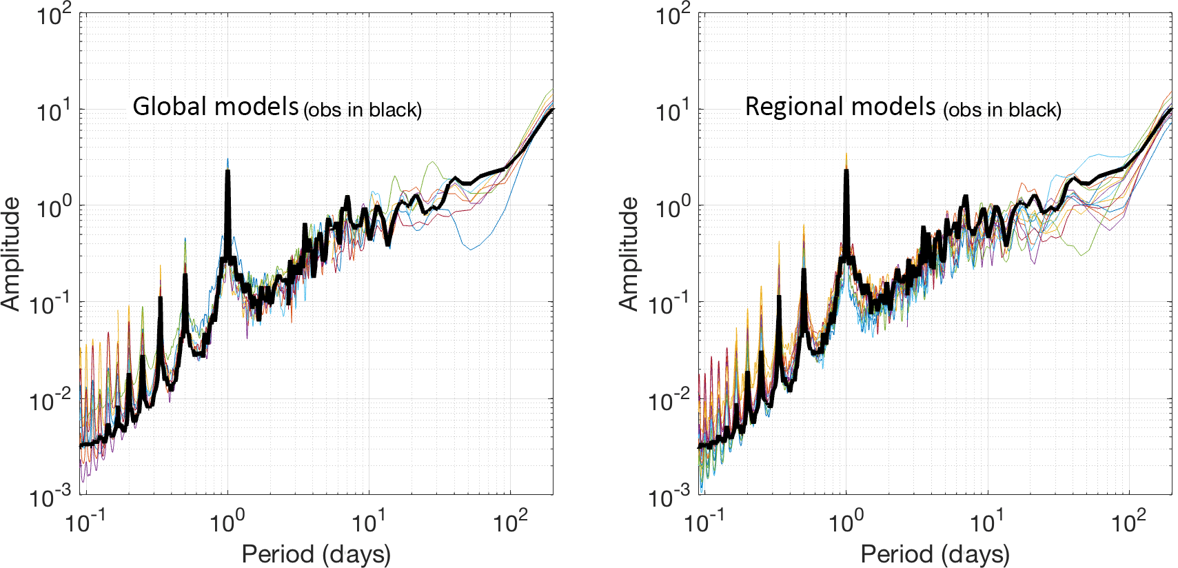
Figure 1Power spectrum of observed ozone (thick line) obtained from the average 1-year time series across all measuring locations and of global models and regional models.
Hourly modelled concentrations of ozone were extracted by the modelling groups at European routine and non-routine sampling locations presented in Fig. S1 of the Supplement. Details on the networks used can be found in Solazzo et al. (2012a, b), Im et al. (2015) and Solazzo et al. (2017). Surface data were provided by the European Monitoring and Evaluation Programme (EMEP; http://www.emep.int/, last access: 18 June 2018) and the European Air Quality Database (AirBase; http://acm.eionet.europa.eu/databases/airbase, last access: 18 June 2018). For the purposes of comparing the ensemble performance with observations, only rural stations with data completeness greater than 75 % for the entire year and elevation above ground lower than 1000 m have been included in the analysis. The total number of valid time series used is 405. Only rural stations have been selected as they capture more background signal than local effects. Including urban and suburban stations in the analysis would penalize global models, which will not be able to capture local effects on ozone.
3.1 Spectral analysis of the global and regional model time series of ozone concentrations
One year of 1 h resolution ozone data allows us to produce detailed spectra from the two groups of models and the measured concentrations. In Fig. 1, the individual power spectra of ozone (plotted against the period in days for easier interpretation) from global and regional models are compared with the spectrum of the measured ozone. The time series of the rural monitoring stations have been averaged prior to producing the spectra. In almost all subsequent results, the measured time series should be interpreted as ensemble averages of all available rural monitoring stations with 1h temporal resolution. The analysis was not performed with spatially aggregated time series only in Figs. 7, 9 and 11, while a subset of the annual hourly time series was used in Fig. 8 (June–August).
Since ozone is a scalar quantity, its spectrum grows monotonically in log–log scale as expected (e.g. Galmarini and Thunis, 2000), showing a distinct peak around a period of 24 h, corresponding to the daily boundary layer evolution and photochemical production of ozone. This peak is captured well by the two groups of models. The global set tends to slightly underestimate the energy associated with this period, with only a single model that overestimates it. The regional-scale models are evenly distributed around the spectrum of the measured time series. The two groups behave remarkably similarly at scales smaller than the daily peak. The majority of the models overestimate the energy but capture the slope of the measured spectrum. As expected, the spectra of the global models are more scattered but yet very well behaved. A weak second peak is visible between 30 and 50 days, which could be easily attributed to the synoptic variability. Solazzo and Galmarini (2015) demonstrated that it could indeed be connected to meteorology and/or removal by dry deposition. Moving up the period scale, after the daily peak, all regional-scale model spectra are below the observed spectra, a behaviour that continues apart from a few exceptions up until the 60–70 day-period range. Out of seven global models however, only three under- or overestimate the energy in this period range, while the rest matches the observed spectrum. At 70–80 days a new peak appears in the observed time series, corresponding to the seasonal variability. Only one global model captures the observed time series; three models seem to anticipate it at smaller periods, and even in the regional-scale group there are a variety of behaviours including a monotonic increase of the energy throughout this period range. Beyond the 100-day period the ozone energy spectrum grows monotonically. The global model group matches the power line in trend and value very closely, whereas the regional scale group shows a more erratic behaviour.
This first test is important to assess the fundamental differences between the two sets of models with respect to the characteristics of the signal, the periodicities present in the latter and the ability to reproduce the power or the variance of the measured signal at the various frequencies (periods). In addition, it can give us an idea of the level of complementarity that exists between the two groups of models in the representation of the measured power spectrum. As clearly evident from Fig. 1, both groups of models show an internal coherence in the representation of the power spectra. A remarkable result is the capacity of global models to represent the high-frequency part of the ozone spectrum with an accuracy that is comparable with regional models. We can expect a complementarity in the behaviour of the two groups in the large-scale energy range, which should be regulating the long-range transport and background values. The global models have a better representation of that portion of the spectrum than the regional one.
3.2 Group performance and error apportionment
A characterization of model performance for the individual members of the two groups beyond the information provided in Solazzo et al. (2017) and Solazzo Galmarini (2015) is also appropriate at this stage.
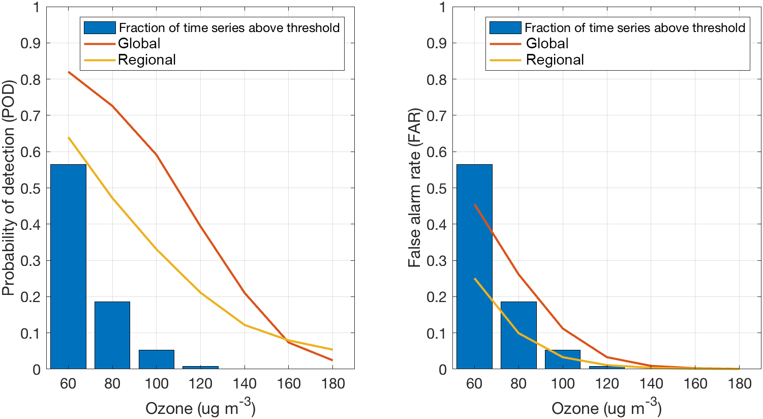
Figure 3Cumulated probability of detection (POD) and false-alarm rate (FAR) for global and regional models at various ozone concentration threshold.
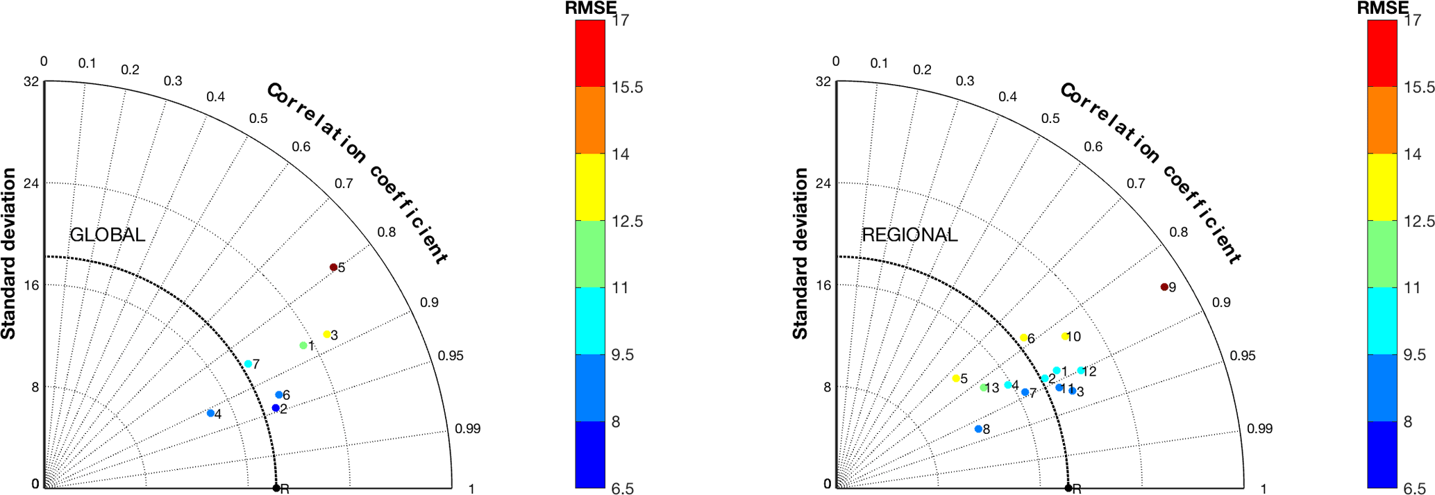
The Taylor diagrams presented in Fig. 2 provide an overview of the individual model performance across the year of reference. All model results underwent un-biasing (subtract the annual mean bias from the predicted hourly values, which produces a shift of the annual time series up or down by mean bias). We notice that the global models show a more scattered behaviour compared to the regional-scale models, with performance distributed across a wider range of standard deviation values. Among the global-scale models we find a clear outlier (model 5), whereas the rest tend to group in a rather narrow range of standard deviation values and correlations. Among the regional-scale models we can also identify an outlier, specifically model 9. The average root mean square error (RMSE) values over all stations ranges from 22.4 to 25.9 µg m−3 for the global models and 21 to 24.7 µg m−3 for the regional models and are thus comparable. Global models overestimate the observed standard deviation, while regional-scale models with the exception of model 9 are evenly distributed across the observed values. The correlation coefficient is comparable for the two groups of models.
Figure 3 presents two classical skill scores for categorical events also applied by Kioutsioukis et al. (2016), namely the probability of detection (POD) and false-alarm rate (FAR). The former represents the proportion of occurrences (e.g. events exceeding a threshold value) that were correctly identified, whereas FAR is the proportion of non-occurrences that were incorrectly identified. In other words they measure true and false positives. In this case the scores are calculated on the basis of the individual model performances at each station. POD and FAR plots are presented as probabilities above breakdowns for different threshold values, where the abundance of the observed data per concentration range is also given as a histogram. A binned analysis of the RMSE (Fig. S2) demonstrates that global models achieve lower RMSE at concentrations above 100 µg m−3; the opposite is true for concentrations below this threshold. This partially explains the facts of Fig. 3.
At the same time the global models also have a higher percentage of false positives as can be gleaned from the FAR index. This analysis is important to establish the capacity of the models to simulate extreme values.
Using the methodology proposed by Galmarini et al. (2013), in Fig. 4 we present the decomposition of the model errors according to specific timescales. In this figure, the individual model errors are shown as decomposed in the diurnal (< 6 h), inter-diurnal (6 h–1 day), synoptic (1–10 days) and long-term (> 10 days) timescales and the residual. The decomposition is performed using a Kolmogorov–Zurbenko filter (Rao et al., 1997) applied to the mean squared error (MSE) calculated from each model and the observed ozone time series. Such analysis can be very revealing as it identifies the scale and therefore the processes that are mainly responsible for the deviation of the model results from the measurements as well as possible persistence of errors at specific scales.

Figure 4Distribution of the mean square error (MSE) across the models of the two communities and the scales on which the signal has been decomposed (LT, long term; SY, synoptic; DU, diurnal; ID, inter-diurnal; see text for definition).
The figure reveals that most of the error is contained in the long-term and diurnal timescales. For regional-scale models, this is in agreement with the findings of Galmarini et al. (2013), Solazzo and Galmarini (2015) and Solazzo et al. (2017). The same behaviour is also found in the group of global models. What is remarkable is the similarity of the error values at the diurnal timescale across the two groups. This suggests that the difference in spatial resolution between the two sets of models does not seem to influence the error at the scale at which atmospheric boundary layer dynamics and daily emissions of ozone precursors are the dominant processes. Apart from a few exceptions (models 13 and 17 in the regional-scale group and models 1 and 5 in the global-scale group), all other models have very comparable errors at that scale. A comparable error across the two groups is found at the synoptic scale, although this is less surprising because this scale is explicitly resolved by the models in both groups and strongly depends on the quality of the meteorological driver used. Since both global and regional models employ assimilation of meteorological observations, they are able to represent the synoptic scale comparably and are less dependent on parameterizations employed. The long-term components have the largest error and also show the most variability across models. Remarkably, the regional-scale models seem to show smaller long-term error values than the global models, although the former show highly variable model-to-model errors. The strong dependence of the long-term error on boundary conditions (specifically lateral boundary conditions for regional-scale models and long-range transport in the case of a global model, upper-stratospheric air intrusions and surface emission of ozone precursors and direct ozone deposition) appears to influence the global-scale group concentrations more than the regional scale, though one should consider that almost all regional-scale models used boundary conditions from the same global model, which nevertheless does not have the smallest long-term error component.
A useful pre-characterization of an ensemble can be obtained by the construction of the Talagrand diagram (Talagrand et al., 1999). It is achieved by binning the range from the minimum to the maximum modelled concentrations with as many bins as the number of ensemble members plus 1. The bins are then filled with observed values accordingly. For example, if an observed value is lower than the lowest model value, it is assigned to the first bin; if it falls between the lowest and second-lowest model value, it is assigned to the second bin; and so on. If it exceeds the highest model value, it is assigned to the last bin. Figure 5 shows the Talagrand diagrams for the global and regional and the regional+global set of models. The figures reveal the tendency of the global model ensemble to be overdispersed as indicated by the accumulation of most of the observed data at the centre of the histogram and relatively few observations falling into the more extreme modelled bins. The regional-scale model ensemble shows a flat diagram, which is an indication of good group performance. A flat Talagrand diagram is an indication of the fact that the group members equally cover (by proportion) all the observed range of values, and the group variability does not show an excess or deficiency in the number of predictions in a specific range of observed values.

Figure 5Talagrand diagrams of global models, regional models and the global+regional set of model results.
The first result obtained for a combined set of model results is shown in the third panel of Fig. 5, which presents the Talagrand diagram for the combination of the two groups of models. Note that the number of bins (x axis) has increased, corresponding to the new total number of models considered plus 1 (i.e. 7 global models plus 13 regional models plus 1). The diagram for the combined group of models qualitatively constitutes an improvement compared to those of the individual group ensembles. The combination of the bell-shaped diagram of the global set with the relatively flat shape of the regional set produces a new distribution within the range of modelled values of the observation, showing a flat region between bins 5 and 18 and an under-prediction region between bins 1 and 5 and bins 19 and 21, which now account for lower and higher values respectively compared to the same bins of the global and regional sets.
4.1 Ensemble analysis per scale group
Prior to analysing the performance of the hybrid multi-model ensemble (mme_GR), let us concentrate on the individual ensembles (mme_R and mme_G) of the two groups for the sake of having an extra term of comparison beyond the measured concentrations against which to compare mme_GR. In this study, we would also like to build upon the research performed in other multi-model ensembles over the years; rather than calculating only the classical model average or median ensemble (mme), we shall also calculate three ensembles based on the findings of Potempski and Galmarini (2009), Riccio et al. (2012), Solazzo et al. (2012a, b, 2013), Galmarini et al. (2013), and Kioutsioukis and Galmarini (2014). We shall therefore refer to the ensemble made by the optimal subset of models that produce the minimum RMSE as mmeS (Solazzo et al., 2012a, b); the ensemble produced by filtering measurements and all model results using the Kolmogorov–Zurbenko decomposition presented earlier and recombining the four components that best compare with the observed components into a new model set as kzFO (Galmarini et al., 2013); and the optimally weighted combination as mmeW (Potempski and Galmarini, 2009; Kioutsioukis and Galmarini, 2014; Kioutsioukis et al., 2016).
Figure 6 shows the effect of the various ensemble treatments for the two groups of models separately and presented as a Taylor diagram. The correlation has increased and narrowed between 0.90 and 0.95 for both groups. As expected, the best ensemble treatment of the two individual groups is mmeW, which in the case of the global models is comparable to mmeS and in the case of the regional-scale models is farther apart from mmeS. The fact that the optimal partition of the error in terms of accuracy and diversity in an equally weighted sub-ensemble (mmeS) and the analytical optimization of the error in a weighted full-ensemble (mmeW) are comparable for the global models implies that this group better replicates the behaviour of an independent and identically distributed (i.i.d., represented by the square in all panels) ensemble around the true state set (on average). The range of improvement of the RMSE is comparable for the two groups of models.
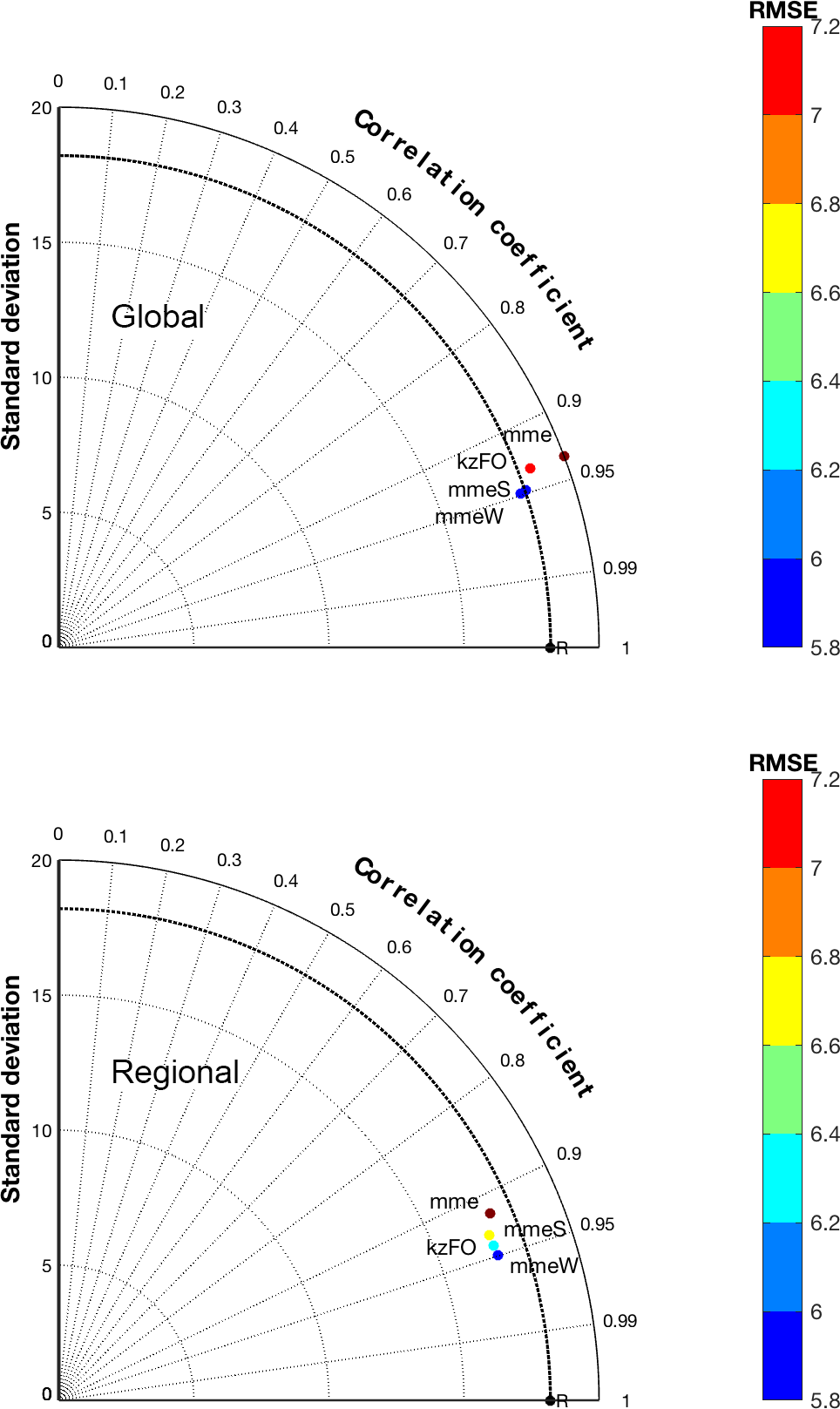
Figure 6Taylor diagram of the four ensemble treatments considered in the text obtained from the global and regional models.
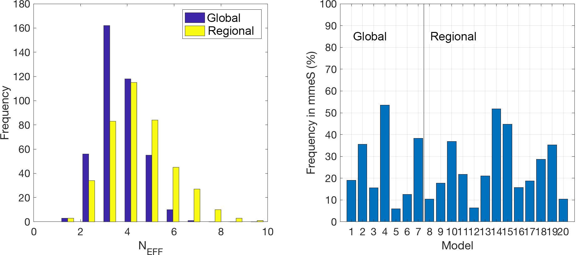
Figure 7Effective number (Neff) of models calculated according to Bretherton et al. (1999) for the two groups of models, and frequency of contribution of each model to the mmeS.
Of the entire set of ensemble treatments proposed, mmeS is the only one that works with an identified subset of elements. The elements chosen in this context are those that minimize a specific metric (e.g. RMSE). The combination of all possible permutations of a pre-defined subset and for all possible subsets allows us to identify the subgroup of models that performs best (Solazzo et al., 2012a, b). This group is the one that best reduces the redundancies and optimizes the complementarity of the model results (Kioutsioukis and Galmarini, 2014). Other methods have been devised to determine the optimal number of models (Bretherton et al., 1999; Riccio et al., 2012) that are equally effective as the one used here, though they do not allow identifying the members of the subset. Beyond the use of the mmeS for the current analysis, given the diversity in the number of models comprising the two ensembles we have calculated the effective numbers of models (Bretherton et al., 1999) for the regional and global sets in the attempt to verify whether the effective numbers were close for the two sets. Figure 7 shows the Neff obtained for the global set and the regional set. At over two-thirds of the stations, the mmeS used three to four global models and three to five regional models. In other words, roughly half of the global models (3–4 out of 7) produce the best result when constructing the mmeS globally, while in the case of the regional-scale models less than half (3–5 out of 13) of all models are required. Figure 7 also provides the frequency of contribution of the individual models to the mmeS, thus confirming the dominance of three global and four regional models determined with the Neff analysis. What is presented in Fig. 7 is the analysis for the aggregated set of model results at all available monitoring points. We also would like to determine the spatial variability of this result, i.e. to answer the question of whether Neff is uniform throughout the domain or whether there are sub-regions that require more or fewer models to construct mmeS.
In order to have a more objective assessment of the result presented in Fig. 7, we introduce a metric which samples only the diversity of the model results (see Sect. 4.3). Following Pennel and Reichler (2011) and Solazzo et al. (2013) we introduce the metric dm, defined for M models at location i as
where
and the ∗ version of em,i and mmei is obtained by normalizing them with σe and σmmei respectively. Rm,mme is the correlation between the individual and average model results. Therefore only the uncorrelated portion of the individual result is retained in dm as a measure of the diversity, whereas the correlated portion is filtered out. Applying this metric, the model results have been decomposed by means of the Kolmogorov–Zurbenko filter described earlier, and Neff has been calculated across the domain for the most relevant components – long term (> 4 days, LT), synoptic (< 4 days, SY) and diurnal (< 1 day, DU) – according to the definitions presented by Solazzo et al. (2017) and references therein. Figure S3 presents the results for the two groups of models. For the long-term component, Neff results shown in Fig. 7 are largely confirmed with an overall spatial homogeneity of Neff. The global model set appears to require a larger number of models than the average in critical areas like northern Italy, where the resolution would be insufficient to capture the inhomogeneity of the concentration field due to the complex terrain in that region (similarly in the western part of the domain). At the synoptic scale, the regional-scale models require slightly more models on average than the numbers presented in Fig. 7, and in some portions of the domain almost all available models are required. The number of required models increases even further at the diurnal scale. In the case of the global set, the average Neff is the same across these two scales, and more models are required in the Po valley (Italy) at the synoptic scale and western Poland at the diurnal scale.
4.2 Building the hybrid ensemble
Given the fact that there is redundancy in the two groups of models and a disparity exists in the overall and effective number of models in the two groups, a strategy has to be devised so that no pre-determined weight is assigned to one of the two groups, thus masking the potential outcome of this study or creating false results. This goal is accomplished by applying the following strategy.
We want to compare three equally populated ensembles of just global, just regional, and mixed global and regional models. We will therefore reduce the ensemble of regional-scale models and include extra models in the ensemble of global models beyond the effective number calculated in Figs. 7 and S3 so that the joint ensemble will not be too small. In order to accomplish this, we select the global models contributing most to the global ensemble beyond those identified by Neff. We begin by assuming that six models comprise a reasonably abundant ensemble (as also indicated by the effective number of regional-scale models), and as such the single-scale ensembles will be based on six members. Taking advantage of the various techniques developed to build an ensemble presented earlier, we define the following sets:
-
(mme_GR) hybrid ensemble of rank 6 (ensemble of six members) composed of the three best global models and the three best regional models
-
(mme_G) global ensemble of six best global models
-
(mme_R) regional ensemble of six best regional models
-
(mmeS_GR) optimally generated hybrid ensemble of rank 6 from the pool of the six best global models and the six best regional models
-
(mmeS_G) optimal global ensemble of rank 6
-
(mmeS_R) optimal regional ensemble of rank 6
-
(mmeW_GR) weighted hybrid ensemble composed of the three best global models and the three best regional models
-
(mmeW_G) weighted global ensemble of six best global models
-
(mmeW_R) weighted regional ensemble of six best regional models
Among them, the mmeS_GR is the only ensemble product that allows unbalanced contributions from global and regional models.
4.3 Comparing the single-scale multi-model ensembles with the hybrid one
The comparison of the ensemble performances will be restricted to the months of June–August, when the photochemical production of ozone is at its maximum and the number of exceedances is expected to peak throughout the continent. The results of the comparison of the mme, mmeS and mmeW for the regional (_R), global (_G) and hybrid cases (_GR) are shown in Fig. 8. The elements common to the three panels are as follows:

Figure 8Comparison of the performance of three ensemble treatments (mme, mmeS and mmeW) for three groupings of models (regional – R; global – G; and mixed global and regional – GR).
-
The hybrid ensemble of rank 6 composed of the three best global models and the three best regional models (mme_GR) when compared to mme_G (best six global models) and mme_R (best six regional models) does not show improved performance; rather its skill is inferior to both mme_G and mme_R.
-
For the other two kinds of ensemble treatments (mmeS and mmeW), the combination of global and regional models produces some improvement compared to just the global or regional ensembles in terms of correlation coefficients, standard deviations and RMSE.
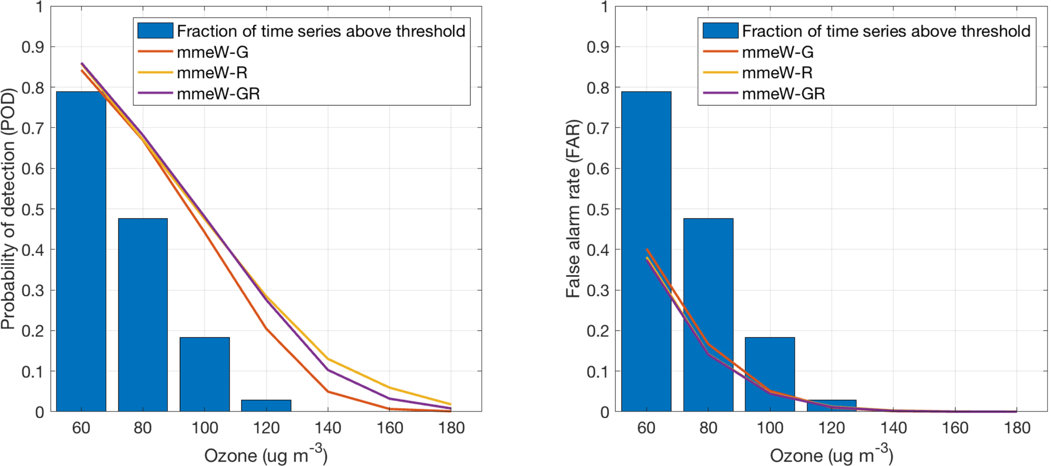
Figure 10POD and FAR for the best-performing ensemble treatment (mmeW) and for three ensemble grouping (regional – R; global – G; and mixed global and regional – RG).
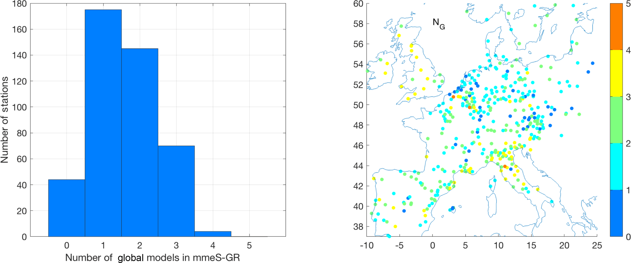
The partition of global and regional models in mmeS (Fig. 9) shows that the contribution of regional models is more frequent. Specifically, at two-thirds of the stations, the optimum hybrid ensemble of rank 6 consists of one or two global models and five or four regional models respectively. At only 15 % of the stations, mmeS consists of an equal number of global and regional models. The maximum number of global models in the mmeS_GR ensemble is four, achieved at roughly 1 % of the stations. Conversely, at around 10 % of the stations the hybrid ensemble utilized only regional models. The second panel of Fig. 9 also gives the spatial distribution of the number of global models contributing to the hybrid ensemble, clearly indicating a preference for regional models in the northeastern part of the domain. This “spatial” preference is not observed in the JJA hourly time series or the annual daily maximum time series (Fig. S4), both being high-ozone datasets. This is in line with the relatively higher RMSE of the global models at low concentrations (Fig. S2).
In Fig. 10, POD and FAR show a net improvement over the mmeW_G results when the hybrid ensemble is considered, with a minimum in false positives and a maximum in true positives that closely match the mmeW_R results.
The real improvement of the hybrid ensemble with respect to the single-scale model ensembles becomes evident when analysing Fig. 11. The panels in the figure are the collective representation of three of the most important characteristics of an ensemble as proposed by Kioutsioukis and Galmarini (2014), i.e. diversity, accuracy and error. On the x and y axes respectively “diversity” and “accuracy” are presented. The former represents the average square deviation of the single models from the mean of the models, whereas the latter is the square of the average deviation of the individual model results from the observed value. As presented by Krogh and Vedelsby (1995), the difference of the diversity and accuracy defines the quadratic deviation of the ensemble average from the observed value. From the definition it follows that, in order for the ensemble result to be closer to the observed value, one has to find the right trade-off between accuracy and diversity (A–D). A mere increase in diversity does not guarantee a minimization of the ensemble error since it might produce a reduction in the accuracy. What one hopes to obtain is the right combination of models that provides the maximum accuracy and maximum diversity. In the plots of Fig. 11, the optimal condition is achieved when the model results are concentrated in the upper left quadrant of the plot toward the (, y=1) point. In the plot, the accuracy parameter is presented as a deviation from the best model performance. The dots represent the estimate of the two parameters at every location where measurements are available. The colour scale is based on the RMSE. The two upper panels give the A–D mapping for the mme_R and mme_G ensembles; the lower two panels give the map for the hybrid ensembles, i.e. mme_GR and mmeS_GR. The difference in nature of the two ensembles is clear from the two panels. Ensemble mme_G is less diverse and more accurate than mme_R (x values: 69 in G and 66 in R; y: 0.75 in G and 0.66 in R). The combination of the two ensembles produces an improvement only in diversity (mme_GR). However, if the models are selected as in mmeS, both accuracy and diversity increase (mmeS_GR). The real advantage of the combination is visible in a slight increase of the diversity as compared to mme_GR and a marked improvement of the accuracy from 0.70 to 0.81. The error decreases from a median value of 17.9 to 15.6 and from an interquartile range of 5.1 to 3.8.
Table 3The fractional change achieved in accuracy, diversity, RMSE, POD and FAR when moving from single-scale to multi-scale ensembles. Results consider the optimal ensembles of rank 6, at hourly or daily maximum resolution.
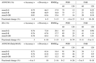
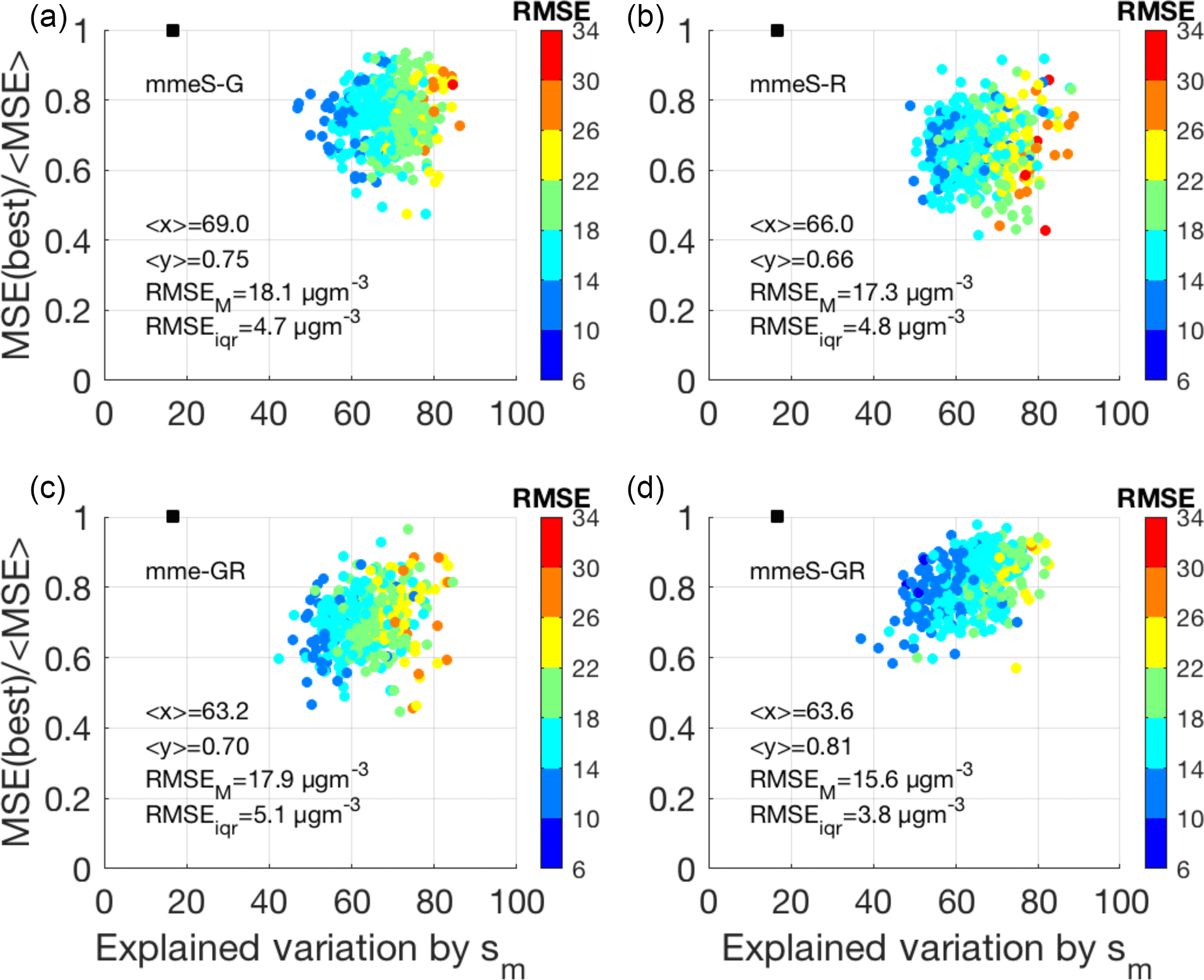
Figure 11Representation of the accuracy (y axis) vs. diversity (x axis) and RMSE for the ensemble of the six most contributing global (a) and regional models (b), and a hybrid ensemble calculated with mme and mmeS ensemble methods (c, d). For reference, the square represents the ideal point corresponding to an independent and identically distributed models (i.i.d ensemble). If the models are i.i.d., then all eigenvalues are equal, each explains 1∕N of the variance and therefore for six models the point is at (0.16; 1). RMSEM is the median root mean square error, while RMSEiqr is the interquartile RMSE.
To answer the question of whether the multi-scale ensemble is more skillful, we consider the two optimal single-scale ensembles of rank 6, namely the global (mmeS-G) and the regional (mmeS-R), and the optimal multi-scale ensemble of rank 6 (mmeS-GR) that is constructed from elements of the optimal single-scale ensembles. The multi-scale ensemble achieves an improved diversity by at least 4 % compared to the single-scale ensembles, even reaching 10 % for the daily maximum time series (Table 3). It reflects the independent development of global and regional models. The change in accuracy is generally smaller since the optimal single-scale pool contains models with not very different errors. When the two pools are combined, the mmeS-GR achieves a better RMSE by 13–16 % compared to mmeS-G and by 2–3 % compared to mmeS-R. Further, the mean of the distributions of diversity, accuracy and RMSE from mmeS-GR differs from the corresponding mean of mmeS-G and mmeS-R (they passed the t test at the 5 % significance level). The same holds for the distributions (they passed the Kolmogorov-Smirnov test). Improvements are also revealed for the POD and the FAR, where the mmeS-R does better than mmeS-G, especially at high thresholds. The mmeS-GR generally improves the indices compared to mmeS-R, even though global models are included. Like before, the improvements are seen in all datasets, despite their temporal aggregation.
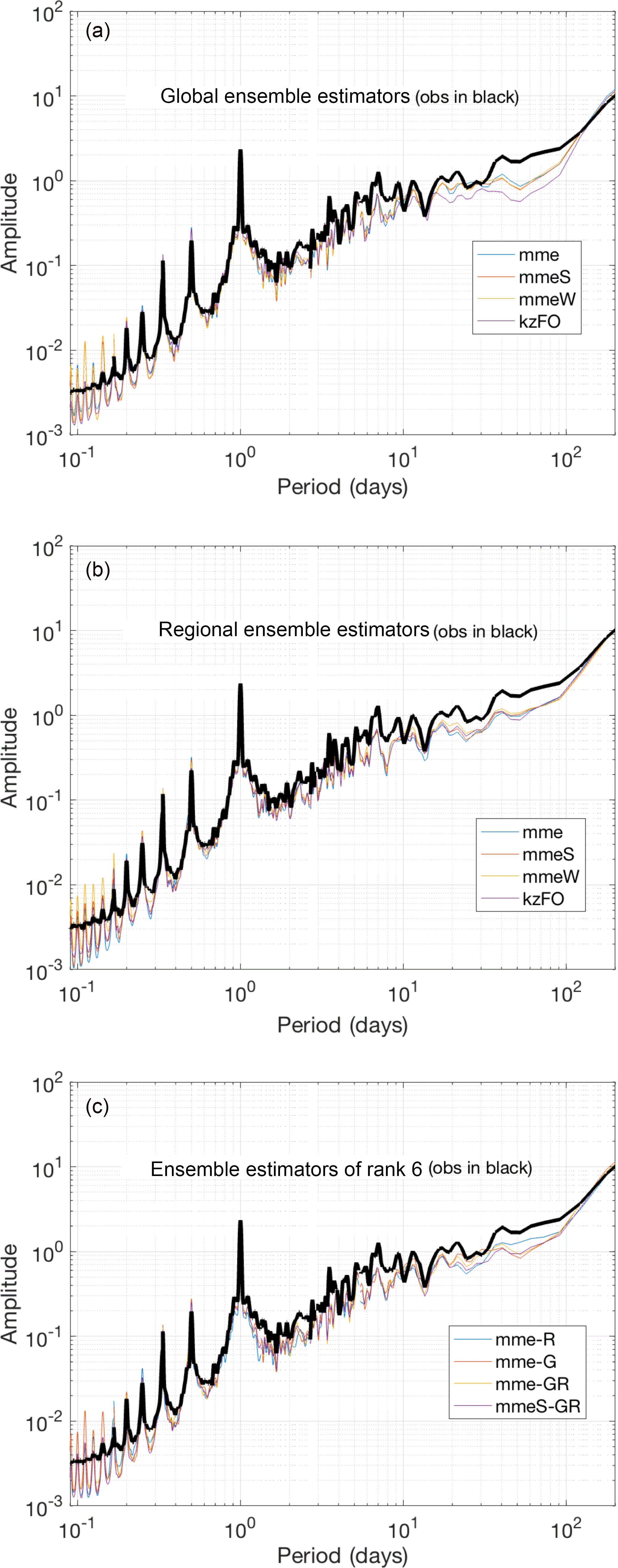
Figure 12Spectra behaviour of the ensemble treatments: full global ensemble (a); full regional ensemble (b); mme of the six most frequently present global and regional models and the hybrid ensemble calculated with mme and mmeS ensemble methods (c).
In Fig. 12 the spectra of the ensembles are presented. For the just-global- and just-regional-scale ensembles, and the rank 6 hybrid ensemble, the spectra of mme, mmeS, mmeW and kFO (Kolmogorov–Zurbenko first order) are shown in the figure. Figure 12 also shows the spectra of the four ensembles (mme_R6, mme_G6, mme_GR6 and mmeS_GR6) for which the six largest contributors from the regional models, the six largest contributors from the global models, and three regional plus three global models were used. From the picture we see that, regardless of the treatment, the ensemble data capture the ozone power spectrum with no notable deviation from the measured spectrum from one another. It is important to note that an ensemble treatment is a purely statistical treatment that does not consider any physics constraints. The deficiencies that were originally present in the individual model spectra are still present in the ensemble results, particularly the large power deficit in the range from 0.8 days to 100 days. The mme_GR spectrum appears to produce a slight improvement toward filling this energy gap, but the change is very small.
The analysis presented above gives us clear indications that the combination of the two sets of models analysed produces an improvement in the ensemble performance. In particular, the hybrid ensemble appears to be superior to any single-scale ensemble in the optimum setting. For example, given six global, six regional, and three global and three regional ensembles, the optimization always favours the hybrid ensemble. This was repeated for all examined cases: the annual hourly records, the JJA hourly records and the annual daily maximum records.
In terms of quantitative conclusions, comparing the optimal multi-scale (GR) ensemble with the optimal single-scale (G and R) ensembles yielded the following results:
-
Diversity improved at least by 4 % for the hourly time series, becoming 10 % for the daily maximum time series.
-
Accuracy generally improved less than diversity.
-
RMSE improved by 13–16 % compared to G and by 2–3 % compared to R.
-
POD and FAR show a remarkable improvement, with a steep increase in the largest POD values and comparatively smallest values of FAR across the concentration ranges.
Some important considerations need to be taken into account at this point. It is difficult to find quantitative evidence for the fact that the hybrid ensemble improvement can be unequivocally attributed to the multi-scale nature of the ensemble. We have no evidence, nor guarantee, that the same kind of improvement could be reached by adding more regional-scale models to the regional-scale ensemble, or more global models to the global-scale ensemble. However, what is a clear conclusion is that the regional-scale ensemble is characterized by a higher level of redundancy in the members than the global ensemble, since fewer than half of the members produced the optimal ensemble, and that the use of the three best members from the regional-scale ensemble and three best global-scale models produces an improvement in the ensemble performance. This last argument suggests that the addition of more model results of the same “nature” would just contribute to further increase the level of redundancy, while on the other hand the improvement obtained could indeed be attributed to the different “nature” of the global-scale models compared to the regional-scale models.
Therefore, considering
-
the large number of regional-scale models and the spectrum of diversity in their nature (only a small number of the same models were used by multiple groups, and there was an abundance of models developed independently from one another),
-
the relatively smaller number of global model results compared to the regional models and also their different nature,
-
the fact that the two groups of models used the same emission inventories and all the regional-scale models used boundary conditions from the same global model,
one could attribute the improvement of the mmeS_GR ensemble performance to the difference in nature of the two groups and a complementary contribution of the two toward an improved result.
All data used in the this study can be accessed through the JRC ENSEMBLE system (http://ensemble.jrc.ec.europa.eu) upon request to stefano.galmarini@ec.europa.eu.
The supplement related to this article is available online at: https://doi.org/10.5194/acp-18-8727-2018-supplement.
The authors declare that they have no conflict of interest.
The views expressed in this article are those of the authors and do not necessarily represent the views or policies of the U.S. Environmental Protection Agency.
This article is part of the special issue “Global and regional assessment of intercontinental transport of air pollution: results from HTAP, AQMEII and MICS”. It is not affiliated with a conference.
The group from University of L'Aquila kindly thanks the EuroMediterranean
Centre on Climate Change (CMCC) for the computational resources. Paolo Tuccella is
a beneficiary of an AXA Research Fund postdoctoral grant. We acknowledge the
EC FP7 financial support for the TRANSPHORM project (grant agreement
243406). CIEMAT has been financed by the Spanish Ministry of Agriculture and
Fishing, Food and Environment. Dave K. Henze and Yanko Davila recognize support from NASA
HAQAST. The UMU group acknowledges the project REPAIR-CGL2014-59677-R of the
Spanish Ministry of the Economy and Competitiveness and the FEDER
programme for support in conducting this research. The MetNo
work has been partially funded by EMEP under UNECE. Computer time for EMEP
model runs was supported by the Research Council of Norway through the NOTUR
project EMEP (NN2890K) for CPU, and NorStore project European Monitoring and
Evaluation Programme (NS9005K) for storage of data. RSE contribution to this
work has been financed by the research fund for the Italian electrical
system under the contract agreement between RSE S.p.A. and the Ministry of
Economic Development – General Directorate for Nuclear Energy, Renewable
Energy and Energy Efficiency in compliance with the decree of 8 March 2006.
Edited by: Tim Butler
Reviewed by: two anonymous referees
Brandt, J., Silver, J. D., Frohn, L. M., Geels, C., Gross, A., Hansen, A. B., Hansen, K. M., Hedegaard, G. B., Skjøth, C. A., Villadsen, H., Zare, A., and Christensen, J. H.: An integrated model study for Europe and North America using the Danish Eulerian Hemispheric Model with focus on intercontinental transport of air pollution, Atmos. Environ., 53, 156–176, 2012.
Bretherton, C. S., Widmann, M., Dymnikov, V. P., Wallace, J. M., and Bladè, I.: The effective number of spatial degrees of freedom of a time-varying field, J. Climate, 12, 1990–2009, 1999.
Colette, A., Granier, C., Hodnebrog, Ø., Jakobs, H., Maurizi, A., Nyiri, A., Rao, S., Amann, M., Bessagnet, B., D'Angiola, A., Gauss, M., Heyes, C., Klimont, Z., Meleux, F., Memmesheimer, M., Mieville, A., Rouïl, L., Russo, F., Schucht, S., Simpson, D., Stordal, F., Tampieri, F., and Vrac, M.: Future air quality in Europe: a multi-model assessment of projected exposure to ozone, Atmos. Chem. Phys., 12, 10613–10630, https://doi.org/10.5194/acp-12-10613-2012, 2012.
Dentener, F., Keating, T., and Akimoto, H. (Eds.): Hemispheric Transport Of Air Pollution 2010, Part A: Ozone And Particulate Matter, Air Pollution Studies No. 17, Economic Commission For Europe, United Nations, New York, USA and Geneva, Switzerland, 304 pp., 2010.
Fiore, A. M., Dentener, F. J., Wild, O., Cuvelier, C., Schultz, M. G., Hess, P., Textor, C., Schulz, M., Doherty, R. M., Horowitz, L. W., MacKenzie, I. A., Sanderson, M. G., Shindell, D. T., Stevenson, D. S., Szopa, S., Van Dingenen, R., Zeng, G., Atherton, C., Bergmann, D., Bey, I., Carmichael,G., Collins, W. J., Duncan, B. N., Faluvegi, G., Folberth, G., Gauss, M., Gong, S., Hauglustaine, D., Holloway, T., Isaksen, I. S. A., Jacob, D. J., Jonson, J. E., Kaminski, J. W., Keating, T. J., Lupu, A., Marmer, E., Montanaro, V., Park, R. J., Pitari, G., Pringle, K. J., Pyle, J. A., Schroeder, S., Vivanco, M. G., Wind, P., Wojcik, G., Wu, S., and Zuber, A.: Multimodel estimates of intercontinental source-receptor relationships for ozone pollution, J. Geophys. Res., 114, D04301, https://doi.org/10.1029/2008JD010816, 2009.
Flemming, J., Huijnen, V., Arteta, J., Bechtold, P., Beljaars, A., Blechschmidt, A.-M., Diamantakis, M., Engelen, R. J., Gaudel, A., Inness, A., Jones, L., Josse, B., Katragkou, E., Marecal, V., Peuch, V.-H., Richter, A., Schultz, M. G., Stein, O., and Tsikerdekis, A.: Tropospheric chemistry in the Integrated Forecasting System of ECMWF, Geosci. Model Dev., 8, 975–1003, https://doi.org/10.5194/gmd-8-975-2015, 2015.
Galmarini, S. and Thunis, P.: Estimating the contribution of Leonard and cross terms to the subfilter scale from atmospheric data, J. Atmos. Sci., 57, 1785–1796, 2000.
Galmarini, S., Michelutti, F., and Thunis, P.: Estimating the Contribution of Leonard and Cross Terms to the Subfilter Scale from Atmospheric Measurements, J. Atmos. Sci., 57, 2968–2976, 1999.
Galmarini, S., Bianconi, R., Klug, W., Mikkelsen, T., Addis, R., Andronopoulos, S., Astrup, P., Baklanov, A., Bartniki, J., Bartzis, J. C., Bellasio, R., Bompay, F., Buckley, R., Bouzom, M., Champion, H., D'Amours, R., Davakis, E., Eleveld, H., Geertsema, G. T., Glaab, H., Kollax, M., Ilvonen, M., Manning, A., Pechinger, U., Persson, C., Polreich, E., Potemski, S., Prodanova, M., Saltbones, J., Slaper, H., Sofiev, M. A., Syrakov, D., Sørensen, J. H., Van der Auwera, L., Valkama, I., and Zelazny, R.: Ensemble dispersion forecasting – Part I: concept, approach and indicators, Atmos. Environ., 38, 4607–4617, 2004.
Galmarini, S., Kioutsioukis, I., and Solazzo, E.: E pluribus unum: ensemble air quality predictions, Atmos. Chem. Phys., 13, 7153-7182, https://doi.org/10.5194/acp-13-7153-2013, 2013.
Galmarini, S., Koffi, B., Solazzo, E., Keating, T., Hogrefe, C., Schulz, M., Benedictow, A., Griesfeller, J. J., Janssens-Maenhout, G., Carmichael, G., Fu, J., and Dentener, F.: Technical note: Coordination and harmonization of the multi-scale, multi-model activities HTAP2, AQMEII3, and MICS-Asia3: simulations, emission inventories, boundary conditions, and model output formats, Atmos. Chem. Phys., 17, 1543–1555, https://doi.org/10.5194/acp-17-1543-2017, 2017.
Henze, D. K., Hakami, A., and Seinfeld, J. H.: Development of the adjoint of GEOS-Chem, Atmos. Chem. Phys., 7, 2413–2433, https://doi.org/10.5194/acp-7-2413-2007, 2007.
Im, U., Bianconi, R., Solazzo, E., Kioutsioukis, I., Badia, A., Balzarini, A., Baró, R., Bellasio, R., Brunner, D., Chemel, C., Curci, G., Flemming, J., Forkel, R., Giordano, L., Jiménez-Guerrero, P., Hirtl, M., Hodzic, A., Honzak, L., Jorba, O., Knote, C., Kuenen, J. J. P., Makar, P. A., Manders-Groot, A., Neal, L., Pérez, J. L., Pirovano, G., Pouliot, G., San Jose, R., Savage, N., Schroder, W., Sokhi, R. S., Syrakov, D., Torian, A., Tuccella, P., Werhahn, J., Wolke, R., Yahya, K., Zabkar, R., Zhang, Y., Zhang, J., Hogrefe, C., and Galmarini, S.: Evaluation of operational on-line-coupled regional air quality models over Europe and North America in the context of AQMEII phase 2. Part I: Ozone, Atmos. Environ., 115, 404–420, 2015.
Im, U., Brandt, J., Geels, C., Hansen, K. M., Christensen, J. H., Andersen, M. S., Solazzo, E., Kioutsioukis, I., Alyuz, U., Balzarini, A., Baro, R., Bellasio, R., Bianconi, R., Bieser, J., Colette, A., Curci, G., Farrow, A., Flemming, J., Fraser, A., Jimenez-Guerrero, P., Kitwiroon, N., Liang, C.-K., Nopmongcol, U., Pirovano, G., Pozzoli, L., Prank, M., Rose, R., Sokhi, R., Tuccella, P., Unal, A., Vivanco, M. G., West, J., Yarwood, G., Hogrefe, C., and Galmarini, S.: Assessment and economic valuation of air pollution impacts on human health over Europe and the United States as calculated by a multi-model ensemble in the framework of AQMEII3, Atmos. Chem. Phys., 18, 5967–5989, https://doi.org/10.5194/acp-18-5967-2018, 2018.
Janssens-Maenhout, G., Crippa, M., Guizzardi, D., Dentener, F., Muntean, M., Pouliot, G., Keating, T., Zhang, Q., Kurokawa, J., Wankmüller, R., Denier van der Gon, H., Kuenen, J. J. P., Klimont, Z., Frost, G., Darras, S., Koffi, B., and Li, M.: HTAP_v2.2: a mosaic of regional and global emission grid maps for 2008 and 2010 to study hemispheric transport of air pollution, Atmos. Chem. Phys., 15, 11411–11432, https://doi.org/10.5194/acp-15-11411-2015, 2015.
Jonker, H. J., Cuijpers, J. W., and Duynkerke, P. G.: Mesoscale fluctuations in scalars generated by boundary layer convection, J. Atmos. Sci., 56, 801–808, 1999.
Jonker, H. J., Vilà-Guerau de Arellano, J., and Duynkerke, P. G.: Characteristic Length Scales of Reactive Species in a Convective Boundary Layer, J. Atmos. Sci., 61, 41–56, 2004.
Jonson, J. E., Schulz, M., Emmons, L., Flemming, J., Henze, D., Sudo, K., Tronstad Lund, M., Lin, M., Benedictow, A., Koffi, B., Dentener, F., Keating, T., and Kivi, R.: The effects of intercontinental emission sources on European air pollution levels, Atmos. Chem. Phys. Discuss., https://doi.org/10.5194/acp-2018-79, in review, 2018.
Kioutsioukis, I. and Galmarini, S.: De praeceptis ferendis: good practice in multi-model ensembles, Atmos. Chem. Phys., 14, 11791–11815, https://doi.org/10.5194/acp-14-11791-2014, 2014.
Kioutsioukis, I., Im, U., Solazzo, E., Bianconi, R., Badia, A., Balzarini, A., Baró, R., Bellasio, R., Brunner, D., Chemel, C., Curci, G., van der Gon, H. D., Flemming, J., Forkel, R., Giordano, L., Jiménez-Guerrero, P., Hirtl, M., Jorba, O., Manders-Groot, A., Neal, L., Pérez, J. L., Pirovano, G., San Jose, R., Savage, N., Schroder, W., Sokhi, R. S., Syrakov, D., Tuccella, P., Werhahn, J., Wolke, R., Hogrefe, C., and Galmarini, S.: Insights into the deterministic skill of air quality ensembles from the analysis of AQMEII data, Atmos. Chem. Phys., 16, 15629–15652, https://doi.org/10.5194/acp-16-15629-2016, 2016.
Krogh, A. and Vedelsby, J.: Neural Network Ensembles, Cross Validation, and Active Learning, in: Advances in Neural Information Processing Systems, edited by: Tesauro, G., Tourestzky, D. S., and Leen, T. K., MIT Press, Cambridge, USA, 231–238, 1995.
Mathur, R., Xing, J., Gilliam, R., Sarwar, G., Hogrefe, C., Pleim, J., Pouliot, G., Roselle, S., Spero, T. L., Wong, D. C., and Young, J.: Extending the Community Multiscale Air Quality (CMAQ) modeling system to hemispheric scales: overview of process considerations and initial applications, Atmos. Chem. Phys., 17, 12449–12474, https://doi.org/10.5194/acp-17-12449-2017, 2017.
Pennel, C. and Reichler, T.: On the effective numbers of climate models, J. Climate, 24, 2358–2367, 2011.
Pielke Sr., R. A.: Mesoscale Meteorological Modeling, vol. 98 di International Geophysics, Academic Press, San Diego, USA, 760 pp., 2013.
Potempski, S. and Galmarini, S.: Est modus in rebus: analytical properties of multi-model ensembles, Atmos. Chem. Phys., 9, 9471–9489, https://doi.org/10.5194/acp-9-9471-2009, 2009.
Rao, S. T., Zurbenko, I. G., Neagu, R., Porter, P. S., Ku, J. Y., and Henry, R. F.: Space and time scales in ambient ozone data, B. Am. Meteorol. Soc., 78, 2153, https://doi.org/10.1175/1520-0477(1997)078<2153:SATSIA>2.0.CO;2, 1997.
Rao, S. T., Galmarini, S., and Puckett, K.: Air quality model evaluation international initiative (AQMEII): Advancing the state of the science in regional photochemical modelling and its applications, B. Am. Meteorol. Soc., 92, 23–30, 2011.
Riccio, A., Ciaramella, A., Giunta, G., Galmarini, S., Solazzo, E., and Potempski, S.: On the systematic reduction of data complexity in multi-model ensemble atmospheric dispersion modelling, J. Geophys. Res., 117, D05314, https://doi.org/10.1029/2011JD016503, 2012.
Simpson, D., Benedictow, A., Berge, H., Bergström, R., Emberson, L. D., Fagerli, H., Flechard, C. R., Hayman, G. D., Gauss, M., Jonson, J. E., Jenkin, M. E., Nyíri, A., Richter, C., Semeena, V. S., Tsyro, S., Tuovinen, J.-P., Valdebenito, Á., and Wind, P.: The EMEP MSC-W chemical transport model – technical description, Atmos. Chem. Phys., 12, 7825–7865, https://doi.org/10.5194/acp-12-7825-2012, 2012.
Solazzo, E. and Galmarini, S.: A science-based use of ensembles of opportunities for assessment and scenario studies, Atmos. Chem. Phys., 15, 2535–2544, https://doi.org/10.5194/acp-15-2535-2015, 2015.
Solazzo, E., Bianconi, R., Vautard, R., Appel, K. W., Moran, M. D., Hogrefe, C., Bessagnet, B., Brandt, J., Christensen, J. H., Chemel, C., Coll, I., Denier van der Gon, H., Ferreira, J., Forkel, R., Francis, X. V., Grell, G., Grossi, P., Hansen, A. B., Jericvičc, Á., Kraljevic, L., Miranda, A. I., Nopmongcol, U., Pirovano, G., Prank, M., Riccio, A., Sartelet, K. N., Schaap, M., Silver, J. D., Sokhi, R. S., Vira, J., Werhahn, J., Wolke, R., Yarwood, G., Zhang, J., Rao, S., and Galmarini, S.: Model evaluation and ensemble modelling of surface-level ozone in Europe and North America in the context of AQMEII, Atmos. Environ., 53, 60–74, 2012a.
Solazzo, E., Bianconi, R., Pirovano, G., Matthias, V., Vautard, R., Moran, M. D., Wyat Appel, K., Bessagnet, B., Brandt, J., Christensen, J. H., Chemel, C., Coll, I., Ferreira, J., Forkel, R., Francis, X. V., Grell, G., Grossi, P., Hansen, A. B., Miranda, A. I., Nopmongcol, U., Prank, M., Sartelet, K. N., Schaap, M., Silver, J. D., Sokhi, R. S., Vira, J., Werhahn, J., Wolke, R., Yarwood, G., Zhang, J., Rao, S. T., and Galmarini, S.: Operational model evaluation for particulate matter in Europe and North America in the context of AQMEII, Atmos. Environ., 53, 75–92, 2012b.
Solazzo, E., Riccio, A., Kioutsioukis, I., and Galmarini, S.: Pauci ex tanto numero: reduce redundancy in multi-model ensembles, Atmos. Chem. Phys., 13, 8315–8333, https://doi.org/10.5194/acp-13-8315-2013, 2013.
Solazzo, E., Bianconi, R., Hogrefe, C., Curci, G., Tuccella, P., Alyuz, U., Balzarini, A., Baró, R., Bellasio, R., Bieser, J., Brandt, J., Christensen, J. H., Colette, A., Francis, X., Fraser, A., Vivanco, M. G., Jiménez-Guerrero, P., Im, U., Manders, A., Nopmongcol, U., Kitwiroon, N., Pirovano, G., Pozzoli, L., Prank, M., Sokhi, R. S., Unal, A., Yarwood, G., and Galmarini, S.: Evaluation and error apportionment of an ensemble of atmospheric chemistry transport modeling systems: multivariable temporal and spatial breakdown, Atmos. Chem. Phys., 17, 3001–3054, https://doi.org/10.5194/acp-17-3001-2017, 2017.
Sudo, K., Takahashi, M., Kurokawa, J., and Akimoto, H.: Chaser: A global chemical model of the troposphere, 1. Model description, J. Geophys. Res., 107, 4339, https://doi.org/10.1029/2001JD001113, 2002.
Talagrand, O., Vautard, R., and Strauss, B.: Evaluation of probabilistic prediction systems, Workshop proceedings “Workshop on predictability”, 20–22 October 1997, ECMWF, Reading, UK, 1999.
Tebaldi, C. and Knutti, R.: The use of the multimodel ensemble in probabilistic climate projections, Philos. T. Roy. Soc., 365, 2053–2075, 2007.
van der Hoven, I. V.: Power spectrum of horizontal wind speed in the frequency range from 0.0007 to 900 cycles per hour, J. Meteor., 14, 160–164, 1957.
Watanabe, S., Hajima, T., Sudo, K., Nagashima, T., Takemura, T., Okajima, H., Nozawa, T., Kawase, H., Abe, M., Yokohata, T., Ise, T., Sato, H., Kato, E., Takata, K., Emori, S., and Kawamiya, M.: MIROC-ESM 2010: model description and basic results of CMIP5-20c3m experiments, Geosci. Model Dev., 4, 845–872, https://doi.org/10.5194/gmd-4-845-2011, 2011.
Xing, J., Mathur, R., Pleim, J., Hogrefe, C., Gan, C.-M., Wong, D. C., and Wei, C.: Can a coupled meteorology–chemistry model reproduce the historical trend in aerosol direct radiative effects over the Northern Hemisphere?, Atmos. Chem. Phys., 15, 9997–10018, https://doi.org/10.5194/acp-15-9997-2015, 2015.
- Abstract
- Introduction
- The models used and the case study
- Preliminary analysis of the two groups of models
- Analysis of the ensembles and building the hybrid one
- Discussion and conclusions. How much is the improvement attributable to the hybrid character of the ensemble?
- Data availability
- Competing interests
- Disclaimer
- Special issue statement
- Acknowledgements
- References
- Supplement