the Creative Commons Attribution 4.0 License.
the Creative Commons Attribution 4.0 License.
 | 20 Jun 2018
A chemical transport model study of plume-rise and particle size distribution for the Athabasca oil sands
Ayodeji Akingunola
Paul A. Makar
Junhua Zhang
Andrea Darlington
Shao-Meng Li
Mark Gordon
Michael D. Moran
Qiong Zheng
We evaluate four high-resolution model simulations of pollutant emissions, chemical transformation, and downwind transport for the Athabasca oil sands using the Global Environmental Multiscale – Modelling Air-quality and Chemistry (GEM-MACH) model, and compare model results with surface monitoring network and aircraft observations of multiple pollutants, for simulations spanning a time period corresponding to an aircraft measurement campaign in the summer of 2013. We have focussed here on the impact of different representations of the model's aerosol size distribution and plume-rise parameterization on model results.
The use of a more finely resolved representation of the aerosol size distribution was found to have a significant impact on model performance, reducing the magnitude of the original surface PM2.5 negative biases 32 %, from −2.62 to −1.72 µg m−3.
We compared model predictions of SO2, NO2, and speciated particulate matter concentrations from simulations employing the commonly used Briggs (1984) plume-rise algorithms to redistribute emissions from large stacks, with stack plume observations. As in our companion paper (Gordon et al., 2017), we found that Briggs algorithms based on estimates of atmospheric stability at the stack height resulted in under-predictions of plume rise, with 116 out of 176 test cases falling below the model : observation 1 : 2 line, 59 cases falling within a factor of 2 of the observed plume heights, and an average model plume height of 289 m compared to an average observed plume height of 822 m. We used a high-resolution meteorological model to confirm the presence of significant horizontal heterogeneity in the local meteorological conditions driving plume rise. Using these simulated meteorological conditions at the stack locations, we found that a layered buoyancy approach for estimating plume rise in stable to neutral atmospheres, coupled with the assumption of free rise in convectively unstable atmospheres, resulted in much better model performance relative to observations (124 out of 176 cases falling within a factor of 2 of the observed plume height, with 69 of these cases above and 55 of these cases below the 1 : 1 line and within a factor of 2 of observed values). This is in contrast to our companion paper, wherein this layered approach (driven by meteorological observations not co-located with the stacks) showed a relatively modest impact on predicted plume heights. Persistent issues with over-fumigation of plumes in the model were linked to a more rapid decrease in simulated temperature with increasing height than was observed. This in turn may have led to overestimates of near-surface diffusivity, resulting in excessive fumigation.


Forecast ensembles of regional air-quality models tend to have relatively poor performance in their predictions of sulfur dioxide (SO2), with normalized mean biases in the range ±40 %, Pearson's correlation coefficients (R) of less than 0.21, and normalized mean errors of more than 75 % (Makar et al., 2015b). These scores may be contrasted with those for atmospheric ozone (O3) of ±13 % for normalized mean bias, R more than 0.6, and normalized mean errors less than 37 %. SO2 is a primary emitted pollutant (it is not created by photochemical reactions in the atmosphere), with the majority of anthropogenic SO2 emissions in the study region coming from large smokestacks (Zhang et al., 2018). In North America, such “major point sources” are often outfitted with continuous emissions monitoring system (CEMS) instrumentation, which provides accurate hourly estimates of the emitted mass of SO2, as well as estimates of parameters that govern the buoyancy- or momentum-driven rise of the resulting plumes, such as the temperature of the emissions, and their volume flow rate (volume emitted/unit time). Anthropogenic SO2 emissions are the main source of most atmospheric sulfur deposition (Mylona, 1996) (reacting in the gas phase with the OH radical to create sulfuric acid, and in cloud water and rain via aqueous chemistry to create bisulfate and sulfate ions). The poor performance of SO2 predictions in air-quality models is therefore a matter of concern and drives the need to better understand its causes. Some of the potential reasons for this poor performance include (in-)accuracy of the (i) emissions information (less likely in cases where CEMS data are available); (ii) plume-rise parameterization algorithms (which describe the vertical redistribution of the emitted mass according to the stack parameters and meteorological conditions – e.g., Briggs, 1984); (iii) errors in meteorological forecast variables (including wind speed and direction, as well as those used in calculating plume rise); and (iv) SO2 loss processes, such as oxidation (as noted above) and the deposition algorithms and meteorological inputs used for calculating the SO2 deposition rate. Furthermore, a combination of these factors may drive the relative difference in model performance between SO2 and O3; we note, for example, that tropospheric O3 is a secondary pollutant (driven by chemical formation and loss rather than direct emissions of ozone) and hence will be more spatially homogeneous than SO2, with the implication that forecast accuracy for very local conditions will play more of a role in setting the ambient concentrations of SO2 than O3.
The prevalence of CEMS for SO2 observations in both Canada and the United States (EPA, 2018) implies that the CEMS-derived emissions inputs available for model simulations will be well characterized. However, reporting requirements vary between the countries. In Canada, emitting facilities are required to report estimates of their total annual emissions, as well as typical stack parameters, to the federal National Pollutant Release Inventory (NPRI, 2018), although individual Canadian provinces may require more detailed reporting. In the United States, CEMS SO2 data are reported at the national level to the U.S. EPA (EPA, 2015, 2018). In both countries, estimates of the typical stack volume flow rate (and/or the stack exit flow velocity) and effluent stack exit temperatures are reported and used for modelling, instead of hourly estimates recorded by CEMS. In the Canadian province of Alberta, regulatory reporting requirements include CEMS hourly observations of SO2 and NO2 emissions from selected large stacks, as well as hourly information on the stack effluent temperature and volume flow rate.
In our companion paper (Gordon et al., 2017) we note that past and current regional air-quality transport models (Im et al., 2015a; Byun and Ching, 1999; Holmes and Morawska, 2006; Emery et al., 2010) and emissions processing models (CMAS, 2018; Bieser et al., 2011) describe the buoyancy- and/or momentum-driven vertical redistribution of emitted mass from stacks using variations on the work of Briggs (1969, 1975, 1984). In the latter work, observations of plume rise, stack parameter information, and meteorological conditions were used to generate parameterizations, linking these data to the height gained by the centerline of atmospheric plumes (the plume height), as well as the vertical extent of the bulk of the emitted mass about that centerline. However, subsequent early evaluations of the accuracy of these parameterizations (see VDI, 1985) have had mixed results, including parameterization estimates averaging 50 % higher than observations (Gielbel, 1979), within 12 and 50 % of observations (Ritmann, 1982), 30 % higher than observations (England et al., 1976), and 50 % higher than observations (Hamilton, 1967). Recent studies using Reynolds-averaged Navier–Stokes and large eddy simulation modelling have shown that the integral model of Briggs overestimates the plume rise and its overestimation error increases as the role of atmospheric turbulence increases (Ashrafi et al., 2017), as well as underestimates of plume rise, inferred from excessively high predicted surface concentrations (Webster and Thompson, 2002). Our companion paper made use of different sources of meteorological observations to drive the Briggs (1984) plume-rise algorithms, as well as CEMS data and aircraft observations of SO2 plumes from multiple sources over a 29-day period. There we found that the Briggs (1984) plume-rise parameterization significantly underpredicted plume heights in the vicinity of the multiple large SO2 emissions sources in the Canadian Athabasca oil sands, with 34 to 52 % of the parameterized heights falling below half of the observed height, compared to 0 to 11 % of predicted plume heights being above twice the observed height, over conditions ranging from neutral through stable to unstable.
However, in our companion paper we also noted the presence of considerable spatial heterogeneity in the meteorological observations used for the algorithm tests. Temperature profiles and other data used to define the input parameters for the Briggs algorithms were taken from two tall meteorological towers, a windRASS, and a research aircraft and showed a substantial variation in the resulting plume height predictions, despite relatively close physical proximity of these sources of meteorological data (e.g., 8 km distance between the two meteorological towers). The region under study is subject to complex meteorological conditions due to the nature of the terrain (a river valley with up to 800 m of vertical relief, as well as open pit mines and settling ponds which may each be tens of km2 in spatial extent). This heterogeneity cast some uncertainty on the results of the companion paper, in that the best application of the plume-rise algorithms would be driven by the meteorology at the location of the stacks, rather than the location of the available meteorological instruments, and the latter suggested substantial local changes in meteorological conditions. As we show in the sections which follow, the spatial heterogeneity of meteorological conditions has a controlling factor on the predicted plume rise, and, in contrast to our companion paper, an approach making use of local temperature gradients between individual model layers has greatly improved accuracy in comparison to those inferring atmospheric stability conditions from the conditions at the top of the emitting stacks.
These underpredictions of plume rise are a potential source of concern, given that they imply that the underlying algorithms will bias SO2 towards lower concentrations. This will lead to more local rather than long-range sulfur deposition. Sulfur deposition is the focus of other work examining acidifying deposition associated with emissions sources in Alberta (Makar et al., 2018).
The work reported here has four main foci, driven by the need to evaluate and if possible improve the performance of both the algorithms governing plume rise and our air-quality model (Global Environmental Multiscale – Modelling Air-quality and Chemistry; GEM-MACH) which employs those algorithms. The main objectives of this study include (1) an evaluation of the impacts of the plume-rise algorithms on model performance, with the introduction of a new approach to calculate plume rise being compared to the standard Briggs (1984) approach; (2) estimation of the impact of hourly major point stack information on model results; and (3) an overall evaluation of the model performance using different configurations for the representation of plume-rise and particle size distributions.
Table 1A summary of the main physical and chemical processes represented in the GEM-MACH regional model.

2.1 Model overview
Global Environmental Multiscale – Modelling Air-quality and Chemistry (GEM-MACH) is Environment and Climate Change Canada's comprehensive online air-quality and chemical transport modelling system, currently in its second major revision. The model consists of an atmospheric chemistry module (Moran et al., 2010), tightly coupled with the dynamical core and residing within the physics module of the Global Environmental Multiscale (GEM) weather forecast model (Côté et al., 1998a, b; Girard et al., 2014). Emissions for the model are provided using an emissions processing system based on SMOKE – Sparse Matrix Operator Kernel Emissions (Coats, 1996). GEM-MACHv2 is a multiscale model designed and exercised in a wide range of scales, from global chemical transport modelling to regional air-quality modelling with direct and indirect feedbacks between (i) chemistry and meteorology (Makar et al., 2015a, b) and (ii) urban-scale air-quality modelling (Munoz-Alpizar et al., 2017). The physical and chemical processes represented in the model regional air-quality prediction system are summarized in Table 1. The main chemical components are the ADOM-II gas-phase chemistry mechanism using the Young and Boris solver and the aerosol module which includes process representation for particle nucleation, condensation, and coagulation (Gong et al., 2003a, b), and deposition (Zhang et al., 2001). Additional aerosol processes include cloud scavenging and in-cloud aqueous-phase chemistry (Gong et al., 2006), as well as equilibrium inorganic gas-aerosol partitioning (HETV scheme; Makar et al., 2003). Eight aerosol species are included in GEM-MACH: particle sulfate, nitrate, ammonium, primary organic carbon, secondary organic carbon, elemental and/or black carbon, sea-salt, and crustal material. The model also features experimental options for feedback between weather and air quality in 12-bin mode (Makar et al., 2015a ,b). More detailed descriptions of GEM-MACH may be found in Makar et al. (2015a, b) and Im et al. (2015a, b). We discuss elsewhere in this special issue the use of GEM-MACH for acid deposition estimates (Makar et al., 2018), bi-directional fluxes of ammonia to the boreal forest (Whaley et al., 2018), the impact of updated emissions of volatile organic compounds, and organic particulate matter (Zhang et al., 2018) on model performance for these species (Stroud et al., 2018). The vertical transport of heat, moisture, and momentum by turbulent eddies are represented by enhanced vertical diffusion and is based on the turbulent kinetic energy (TKE) closure scheme (Mailhot and Benoit, 1982) in the GEM model physics module. The same numerical scheme and coefficients of vertical diffusivity are used for the diffusive transport of chemical species within GEM-MACH. Table 1 provides an overview of the main processes represented in the atmospheric physics components of the GEM weather forecast model upon which GEM-MACH is based.
2.2 Model setup and configurations
A 2-bin simulation of GEM-MACH running in a nested configuration from a North American 10 km resolution forecast to a 2.5 km Alberta and Saskatchewan domain has been in continuous experimental forecast mode since October 2012, and this configuration is also used for operational forecasts by Environment and Climate Change Canada. While the 2-bin simulation reduces computational processing time by 25 % in the current version of GEM-MACH, we investigate here the effect of this configuration on model accuracy relative to observations, employing the GEM-MACHv2 model in the oil sands 2.5 km nested system using the more detailed 12-bin aerosol size distribution configuration. We have carried out a set of retrospective simulations targeting the JOSM (the Governments of Canada and Alberta Joint Oil Sands Monitoring program) summer 2013 intensive campaign period (JOSM, 2011). The outer 10 km horizontal-resolution domain, which covers most of continental Canada and United States, was configured with 82 vertical levels and a 5 min physics/15 min chemistry time step, with the chemical boundary and initial conditions provided by MOZART-4 climatology (Emmons et al., 2010), and meteorological boundary and initial conditions provided by the GEM-based Regional Deterministic Prediction System (RDPS, Caron and Anselmo, 2014). The RDPS itself was driven by meteorological analyses generated using data assimilation. The RDPS was also used to drive a 2.5 km horizontal-resolution regional weather-only simulation, using a modified GEM High-Resolution Deterministic Prediction System configuration (HRDPS, Charron et al., 2012). Both the modified HRDPS and the 10 km resolution GEM-MACH produced 36 h simulations, the last 24 h of which were used to provide the respective meteorological and chemical boundary conditions for a 24 h GEM-MACH 2.5 km resolution simulation (which was configured with 64 vertical levels, with the underlying meteorology model operating on a 1 min time step and the chemistry module being called every second chemistry step). The use of the HRDPS in this fashion allowed each GEM-MACH 2.5 km simulation to commence from a spun-up state for its cloud variables. For the chemical species, the last hour of each 24 h simulation was used to provide initial conditions for the subsequent GEM-MACH simulation. This provided continuity of the chemical fields across subsequent 24 h simulations. The GEM-MACH 10 km simulation and the HRDPS 2.5 km simulations, updated every 24 h, provided ongoing boundary conditions and hence continuity with the meteorological analysis, thus preventing the high-resolution meteorology from drifting chaotically from the analyses. The GEM-MACH 10km, HRDPS, and GEM-MACH 2.5 km domains are shown in Fig. 1. The retrospective simulations were carried out for the period 1 August 2013 to 10 September 2013, with the first 7 days' results discarded as model spin-up time.
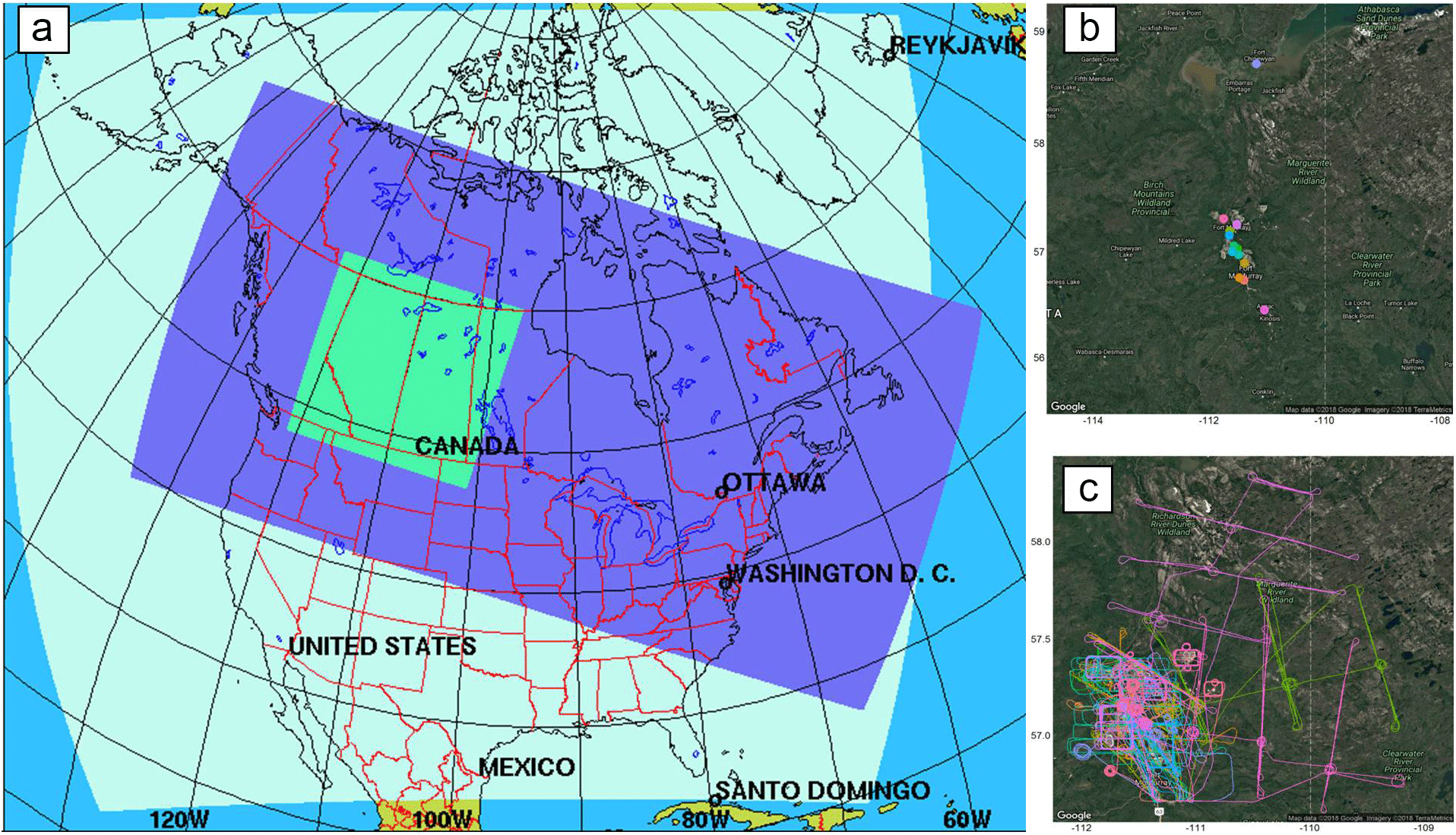
Figure 1Schematic diagram showing the model simulation domains in the nested 2.5 km resolution setup in the right panel. (a) Light blue outermost domain: GEM-MACH 10 km resolution North American forecast. (b) Dark blue domain: HRDPS 2.5 km weather forecast. (c) Green innermost domain: GEM-MACH 2.5 km forecast. Panel (b) is a Google-Earth-referenced image showing the locations of the surface observations used in the study in coloured dots. Panel (c) is a Google-Earth-referenced image showing all 22 flight paths covered during the JOSM 2013 flight campaign.
The emissions used in our simulations were processed from inventory data from different sources, including the Canadian National Pollutant Release Inventory and Air Pollutant Emissions Inventory (APEI) data for 2013, within-facility specific 2010 data from the Cumulative Environmental Management Association (CEMA), and hourly continuous emissions monitoring observations for hourly major point emissions of SO2 and NO2 for the province of Alberta (Alberta Environment and Parks). The latter sources account for 77 and 43 % of total SO2 and NOx emissions, respectively, from all NPRI point sources in Alberta, and 99 and 39 %, respectively, for sources of these compounds solely within the Athabasca oil sands area (Zhang et al., 2018). The same set of emissions was used for all the simulation scenarios carried out for this study. The emissions set is discussed in detail in Zhang et al. (2015, 2018). In the emissions processing, aerosols were chemically speciated for the 12-bin size distribution; the resulting emissions files were summed to the 2-bin distribution for the 2-bin simulations discussed below.
For the purpose of this study we have carried out four sets of model simulations in order to evaluate the impact of (operational) 2-bin versus 12-bin aerosol size distribution, and of different algorithms for plume rise, on model performance.
2.2.1 The 2-bin versus 12-bin model scenarios
Gong et al. (2003a, b) showed that a 12-bin sectional model is sufficient to accurately predict both aerosol number concentration and mass size distributions for most prevalent atmospheric conditions. However, because of the high computational cost and the requirement for a fast turnaround demanded in operational systems, the operational forecast configuration of GEM-MACH employs a 2-bin aerosol size distribution (bins bordered by diameter size cuts 0.01, 2.56, and 10.24 µm), with sub-binning used for those aerosol microphysical processes requiring more detailed aerosol sizing, such as nucleation (Moran et al., 2010). The 12-bin configuration (bins bordered by diameter size cuts 0.01, 0.02, 0.04, 0.08, 0.16, 0.32, 0.64, 1.28, 2.56, 5.12, 10.24, 20.48, and 40.96 µm) has been used for research purposes such as investigating aerosol–weather feedbacks (Makar et al., 2015a, b). Here, both aerosol size distributions were used for 10 and 2.5 km resolution nested simulations. The first two of our simulations are thus referred to as 2-bin and 12-bin, and both make use of the original plume-rise algorithms employed in GEM-MACH (and described below). These simulations were compared to determine the relative impact of the more detailed size distribution on model performance relative to observations.
2.2.2 Plume-rise algorithms: two alternative approaches
As noted earlier, the set of empirical formulations and algorithms developed by Briggs (1984) for evaluating the plume-rise height of major point source emissions has been the basis of plume-rise calculations in several chemistry transport models such as GEM-MACH (Moran et al., 2010) and CMAQ/CMAx (Byun and Schere, 2006), as well as in regulatory air dispersion models such as AEROPOL (Kaasik and Kimmel, 2003) and CALPUFF (Levy et al., 2002). However, the details of how Briggs' algorithms were implemented may vary – we therefore provide the details of the GEM-MACH implementation below. We follow with a revised plume-rise calculation procedure which in our subsequent evaluation is demonstrated to provide a more accurate estimation of final plume height. Our 12-bin simulation noted above makes use of the original algorithm, while we refer to the revised algorithm as plume rise in our subsequent discussion.
The original implementation of the plume-rise algorithm in GEM-MACH is based on the set of equations in Briggs (1984) which calculate the plume-rise height above the top of the emitting stack, Δh, based on the atmospheric turbulence characteristics at the stack location. The formulae rely on a local estimation of the state of the atmosphere in the vertical at that location; the atmospheric stability, temperature gradients, and resulting formulae for plume height are predicated on the assumption that these stack height conditions will continue throughout the atmospheric column until the maximum plume height is reached. However, in cases of more complex atmospheric conditions, where these conditions change significantly with height, the formulae may become inaccurate.
The equations depend on atmospheric stability parameters calculated in the meteorological module of the air-quality model and include the boundary layer height (H), the Monin–Obhukov length (L), the surface wind friction velocity (u∗), the atmospheric temperature (Ta) and its gradient (ΔTa∕Δz), and the wind speed (U) at the stack height. An important parameter in the plume-rise formulations is the emitted plume's initial buoyancy flux (Fb), which is dependent on the stack exit temperature (Ts) and the stack's exit volume flow rate (V), and is given by
where g is the acceleration due to gravity. The emitted plume is buoyant and rises if Ts>Ta; Fb is set to zero if Ts<Ta. If the stack height is within the predicted boundary layer depth (hs<h), the plume rise is calculated based on the stability regimes at the stack height model level by the following equations.
For unstable conditions (),
For stable conditions (),
And for neutral conditions (L>2hs and ),
where is the convective-scale parameter and s is the stability parameter approximated by
where ΔTa∕Δz is the vertical temperature gradient between the atmospheric temperature at the top of the stack and the temperature at the top of the model layer. We note here that some air-quality model implementations make use of one or the other formula of Eqs. (2) and (4), as opposed to the minimum chosen here. In our companion paper (Gordon et al., 2017) we show that these differences have little impact on the calculated plume height.
The model also incorporates the potential for the buoyant plume to penetrate the top of the boundary layer (Hanna and Paine, 1988), which is accounted for by calculating the penetration parameter P and using it to further adjust the plume-rise Δh calculated through the above formulae as
where H is the height of the boundary layer. The plume rise calculated earlier is then reset via
Once the final value of the plume-rise Δh is calculated, the vertical spread of the plume and the emitted mass is then evaluated by using a common method from Briggs (1975) to specify the height of the top and bottom of the plume as
In GEM-MACH, the plume top is further limited to the height of the boundary layer (H), if the penetration P>0. During unstable conditions, the plume bottom is set to zero (the surface); that is, the plume is assumed to mix uniformly throughout the boundary layer. We also note that the mass emitted into the plume is assumed to mix uniformly between ht and hb; this is in contrast to the approach of Turner et al. (1991), wherein a top-hat distribution centred on hs was assumed, or the Gaussian distribution based on unpublished observations described in Byun and Ching (1999).
As described above, the original plume-rise algorithm implemented in GEM-MACH does not account for potential changes in plume rise associated with the vertical variation in the atmospheric temperature and stability, which could be important for plume buoyancy especially during unstable conditions where the boundary layer depth could be much higher than the stack height. Similarly, changes in stability with height will affect plume rise. As reported in Gordon et al. (2017), when meteorological observations collected at oil sands sites are used to drive Eqs. (1) through (5), the estimated plume heights were often underestimated, with between 37 and 52 % of calculated values being less than 1∕2 the observed height.
However, other approaches, which take into account the variation in height associated with atmospheric conditions in the vertical profile above the emitting stack, are available. Briggs proposed equations which would make use of changes in stability between layers and calculate the residual buoyancy flux between layers in the atmosphere – these are particularly amenable to the layered structure of atmospheric models (Briggs, 1984, Eqs. 8.84 and 8.85). This new algorithm is similar to other layer-by-layer approaches available in CMAQ (Byun and Ching, 1999), based on the hesitant-plume algorithm described in Turner et al. (1991) and in dispersion modelling work by Erbrink (1994). In the new algorithm (hereafter referred to as the revised Briggs plume rise or simply plume rise) we utilized the model's calculated vertical profile of atmospheric temperature and wind speed to estimate the plume height as the height at which the emitted plume buoyancy flux dissipates totally. The initial plume buoyancy flux (Fb) at the top of the stack is calculated using Eq. (1) above, by using linear interpolation to evaluate the air temperature (Ta) and wind speed (U) at the stack height from the model's vertical profile. Under (locally) neutral and stable conditions, the buoyant plume is assumed to rise freely, and the residual buoyancy flux (Fr) remaining after it as it crosses the next atmospheric layer is given as follows.
For vertical plumes,
and for bent plumes,
Here, sj is the local stability parameter for a given layer, calculated using Eq. (5) and layer-specific temperature values, and zj is the plume-rise height when the plume reaches the bottom of the model's jth layer. Briggs (1984) recommended the use of both formulae of Eq. (9), with the formula with the greatest decrease in flux being used as the final value. Briggs also noted that the transition to bent plumes happens at a relatively low height above the stack, implying that the residual buoyancy between layers is lost faster under windy conditions. At the stack height, and zj=0 (that is, the vertical distances are relative to the top of the stack). When the residual buoyancy flux becomes negative in Eq. (9), indicating that the plume height has been surpassed, the calculation is repeated to find the value of z for which F=0; the sum of this and the layer thicknesses transitioned to this height become the predicted plume rise. In our companion paper (Gordon et al., 2017), this approach was found to provide similar results to the original Briggs algorithms when driven by observations not co-located with the stacks. Our work here indicates that this algorithm has the potential to provide a more accurate estimate of plume rise, subject to caveats described below.
We note that the numerical coefficients in Eq. (9), 0.015 and 0.053, stem from two parameters: the entrainment constant for vertical rise conditions (α), which is the entrainment coefficient for vertical plumes, nominally set to 0.08 by Briggs based on observations published in 1975 – the parameter in the first equation of Eq. (9) is a non-linear function of this α term; and β′, the entrainment coefficient internal radius for bent-over plumes, set by Briggs to 0.4, though ranges from 0.45 to 0.52 were quoted elsewhere in Briggs (1984). The choice of these parameters is based on data which are now over 40 years old and may present an opportunity for future improvement of this revised plume-rise approach.
The above formula (9) was recommended by Briggs for conditions which are stable to neutral at the stack height. We have defined stability in this case by comparing the dry adiabatic lapse rate to the local temperature lapse rate predicted by the model at the stack height and above. Briggs (1984) provided no equivalent formula for unstable conditions at the stack height, followed by stable profiles at higher elevations. The approach taken here has been to assume under convectively unstable conditions the plume rises without loss of energy (that is, an assumption of zero entrainment) until the predicted temperature profile once again falls below the dry adiabatic lapse rate. Our first order approximation is thus to assume that under unstable conditions there is minimal mixing entrainment of the rising plume with the surrounding atmosphere. This approach differs from that of Turner et al. (1991) and the layered approach described in Byun and Ching (1999) where the residual buoyancy flux between layers is determined using different formulae based on the model-determined local atmospheric stability.
As in the original algorithm, the plume top and plume bottom are evaluated using Eq. (8) after the final plume rise has been evaluated. We do not apply the penetration equations (Eqs. 6 and 7) since these corrections should be unnecessary in an approach making use of local changes in residual buoyancy. In our companion paper, this algorithm was referred to as the layered approach.
2.2.3 Hourly emission stack temperature and volume flow rate
We turn next to the available emissions data for driving the plume-rise algorithms. Under Canadian federal reporting requirements to the National Pollutant Release Inventory, annual total emissions of SO2 and NOx from facilities are reported, along with a single set of stack parameters (stack height, stack diameters, average exit temperature, and average exit velocity) to represent emissions throughout the year. In addition, hourly continuous emissions monitoring data from large stacks are reported to the government of Alberta. These data include the hourly mass of emissions of SO2 and NO2, as well as hourly estimates of the time-varying stack parameters (volume flow rates and temperatures).
2.2.4 Simulation scenarios
Our first two simulations use the standard annual NPRI reported stack parameters and the original plume-rise algorithm for the 2-bin and 12-bin aerosol size distributions, while our second two simulations use the modified plume-rise algorithm, first with the NPRI stack parameters and second with emissions information derived from a combination of CEMS hourly stack parameters as well as engineering estimates of emissions during upset conditions in which the effluent is redirected to flare stacks (the latter estimates are considerably more uncertain than the CEMS information but are nevertheless included here since they result in substantial changes in pollutant emissions and plume characteristics, see Zhang et al., 2018). The four scenarios examined are thus described as follows.
-
A 2-bin simulation: NPRI stack parameters, 2-bin aerosol size distribution, and the original plume rise.
-
A 12-bin simulation: as in (1), but employing the 12-bin aerosol size distribution. Differences between (1) and (2) thus show the impact of the aerosol size distribution on performance.
-
A plume-rise simulation: employing the layered plume-rise algorithm, with emissions as in (2). Differences between (2) and (3) thus show the impact of the revised plume-rise algorithm alone.
-
An hourly simulation: employing the layered plume-rise algorithm, with volume flow rates and temperatures taken from the hourly CEMS data along with upset conditions. Differences between (3) and (4) thus show the impact of the initial buoyancy flux on the resulting plume rise, using the revised algorithm.
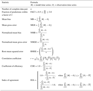
Table 2Statistical measures used in comparing model results with observations.
All of these simulations make use of the CEMS-derived mass of emitted SO2 and NOx.
The comparative statistics presented through this study were computed using the modStat function from the openair R package (Carslaw and Ropkins, 2012) for complete pairs of valid model and observation data. The set of statistical measures and their formulas are presented in Table 2. Both surface monitoring network and aircraft observations have been used for model evaluation.
3.1 WBEA surface monitoring networks
For the purpose of model evaluation, we have used hourly measurements of surface concentrations of PM2.5, SO2, NO2, and O3 from a network of 10 air-quality monitoring stations in the province of Alberta managed by the Wood Buffalo Environmental Association (WBEA) (see Fig. 1b). The observation data have been filtered to remove extreme single-hour measurements that are greater than 150 ppbv for SO2, NO2, and O3, and 150 µg m−3 for PM2.5 (single-hour spikes of this nature in hourly records are assumed to correspond to instrumentation errors or calibration times for the instruments). Observations from 10 August 2013 to 10 September 2013 were selected for comparison to the model results to align with the period covered by the JOSM 2013 intensive aircraft measurement campaign.
3.2 JOSM summer 2013 intensive campaign
From 10 August to 10 September, 2013, the National Research Council of Canada Convair aircraft was used as a mobile measurement platform to sample atmospheric constituents in the region of the Athabasca oil sands, with 22 flights taking place during the given time period (Fig. 1c). These flights included flight paths designed for emission estimation for the study of downwind transport and chemical transformation and for satellite validation. Emission estimation flights took place around individual facilities at multiple altitudes, with the concentration and meteorological information gathered subsequently used to estimate fluxes entering and leaving the facility and hence estimate emissions directly from aircraft observations (Gordon et al., 2015; Li et al., 2017). Transformation flights were designed to follow plumes downwind, with observations taken in cross sections at set distances downwind perpendicular to the plume direction in order to study chemical transformations between point of emission and downwind receptors (see Liggio et al., 2016). Satellite validation flights incorporated aircraft vertical spirals at satellite overpass times in order to improve satellite data retrieval algorithms (Whaley et al., 2018; Shephard et al., 2015). Here, we compare model predictions for our different simulations for SO2, NO2, and for PM1 sulfate, ammonium, and total organics to observations taken on-board the Convair using TS43, TS42, and Aerodyne aerosol mass spectrometer (AMS) instruments, respectively. In order to allow for comparisons to the results from GEM-MACHv2 2.5 km oil sands model domain simulations, 10 s averages of the aircraft's positional data (latitude, longitude, elevation, and time) were created for all 22 flights. These data were in turn used to extract the corresponding linearly interpolated values in time and space from the model's 2 min time step and 2.5 km resolution for each of the species observed aboard the aircraft which were used for the model comparison. The nominal cruise speed of the National Research Council Convair 580 used in the experiment is 550 km h−1; a 10 s time interval thus represents an observation integration distance of 1.528 km, and a 2 min time interval represents an observation integration distance of 18.3 km.
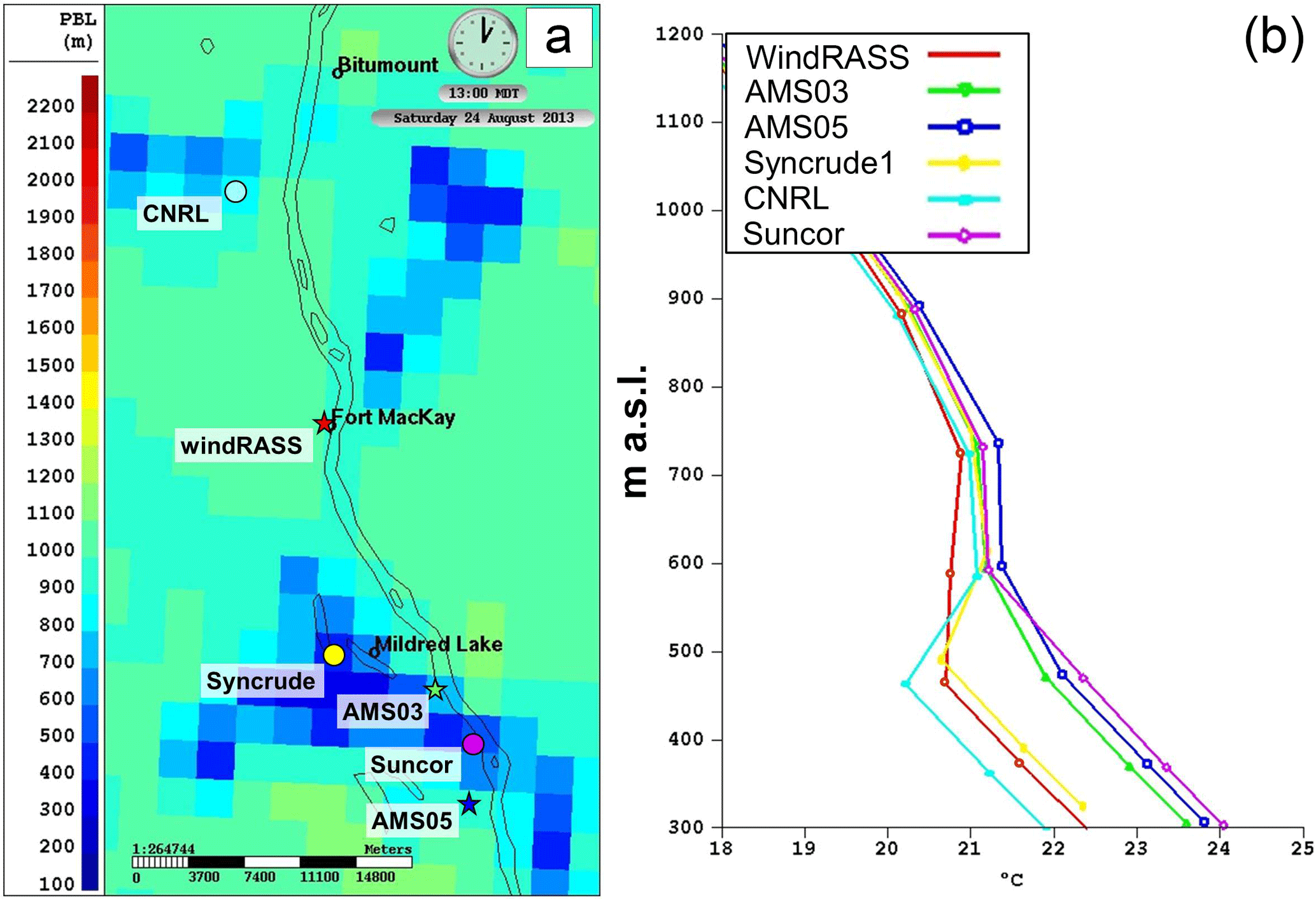
Figure 2Examination of meteorological heterogeneity in the study area. (a) PBL heights (locations of large emitting stacks shown as circles and meteorological observation sites as stars). (b) Predicted temperature profiles at these locations and times; symbols indicate locations of model levels (a terrain-following coordinate system is used in GEM-MACH).
4.1 Spatial heterogeneity of meteorological conditions
We noted in our companion paper (Gordon et al., 2017) that meteorological observations varied substantially in the study region depending on location, citing this as a possible confounding factor on the results of tests of the plume-rise algorithms. This spatial heterogeneity was well captured by the high-resolution GEM-MACH simulations, as is demonstrated by the example depicted in Fig. 2, which shows the typical local variation in planetary boundary layer height (Fig. 2a), ranging from about 1200 to 400 m, with the lower values corresponding to the main cleared areas (open pit mines, settling ponds) of the industrial facilities. The corresponding temperature profiles in several locations marked in Fig. 2a are given in Fig. 2b. These show a substantial difference in model-predicted stability at the three meteorological observation locations of Gordon et al. (2017) (windRASS, AMS03, and AMS05) and substantial differences between these and the locations of the main stacks of some of the facilities (Syncrude 1, CNRL, and Suncor). The temperature profiles show that the height and strength of the inversion may vary by over 100 m in the vertical and that the profiles do not merge with the larger-scale flow until an elevation of 750 m a.s.l. (450 m a.g.l.) is reached. Given this level of variation, we might expect potential errors in calculated plume heights when applying the meteorological observations to plume rise at the stack locations, in turn suggesting that a re-examination of plume rise using the model results is worthwhile.
4.2 The 2-bin versus 12-bin evaluation
We begin our evaluation by comparing the 2-bin and 12-bin particle size distribution simulations using identical emissions against the Wood Buffalo Environmental Association's surface monitoring network PM2.5 measurements. The statistical comparison between these observations and all the four model scenarios is shown in Table 3, and the corresponding histograms of observations (blue), 2-bin model simulated values (red), and 12-bin model simulation values (purple) are shown in Fig. 3. The statistics of Table 3 show that the 12-bin simulation provides an overall improvement over the 2-bin model results across all metrics. For example, the magnitude of the mean bias has decreased from −2.623 to −1.725 µg m−3, a reduction of 34 %, indicating that a sizeable fraction of particulate under-predictions in 2-bin simulations may be due to poor representation of particle microphysics through the use of the 2-bin distribution, despite sub-binning being used in some microphysics processes. The largest improvement in correlation coefficient and fraction of predictions within a factor of 2 also takes place going from the 2-bin to the 12-bin distribution. Figure 3 shows that the model simulations are biased high for PM2.5 concentrations less than 5 µg m−3 and are biased low for higher concentrations. The use of the 12-bin size distribution (purple histogram bars, Fig. 3) improves the fit to the observations (blue histogram bars) in comparison to the 2-bin distribution results (red histogram bars), though significant over-predictions of the frequency of low concentration events and under-prediction of high-concentration events remain.
Table 3Statistical comparison of GEM-MACH model simulation of surface PM2.5 with measurements from the WBEA observations between 10 August and 10 September, 2013. Boldface type indicates best score; italics indicates second best score.
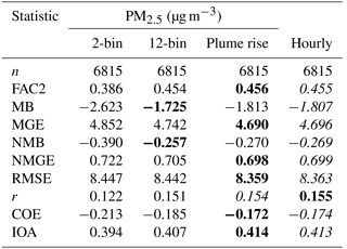
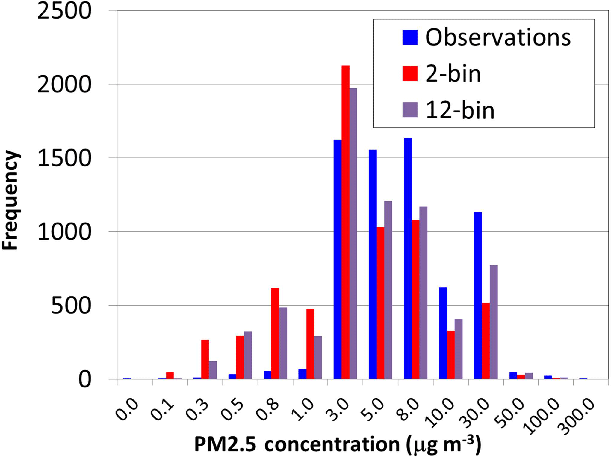
Figure 3Histogram of surface PM2.5 using Wood Buffalo Environmental Association surface monitoring data (blue) and the 2-bin (red) and 12-bin (purple) configurations of GEM-MACH. Both simulations make use of the original Briggs (1984) plume-rise formulation.
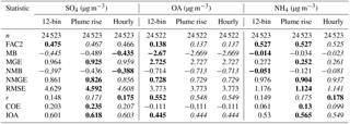
Table 4Statistical comparison of PM1 sulfate, OA, and ammonium atmospheric concentration from the aircraft AMS with the 2.5 km resolution GEM-MACH simulations between 13 August and 9 September 2013. Boldface type indicates best score; italics indicates second best score.
4.3 Plume-rise algorithm evaluation
The simulation with the largest number of highest scores (boldface numbers in Table 3) is the plume-rise algorithm, which made use of the revised plume-rise formulation, though the differences in performance between the 12-bin, plume rise, and hourly simulations are relatively small. The latter small increment is expected, given that the observations are relatively close to the sources of primary particulate emissions, largely from surface sources of fugitive dust (see Zhang et al., 2018). However, an increment of PM2.5 will be from secondary sources; about 99 % of the anthropogenic SO2 and NH3 emissions and about 40 % of the NOx emissions in the Athabasca oil sands region originate in major point source stacks. The concentrations of these precursor species will therefore be influenced by the plume-rise algorithm employed in model simulations, and hence secondary particulate species originating from these primary emissions may also be affected by plume rise. The small improvements in PM2.5 associated with the revised plume-rise algorithm may thus represent the impact of secondary formation of particulate sulfate, ammonium, and nitrate from SO2, NH3, and NOx – the latter having been influenced by the plume-rise treatment. We examine this possibility using observations of PM1 particle sulfate and ammonium taken with an aerosol mass spectrometer aboard the NRCan Convair aircraft.
The aircraft's AMS instrument measures speciated atmospheric particle concentrations for particles less than 1 µm size and therefore cannot be compared with the 2-bin model results because the smaller size bin (with upper diameter size cut 2.56 µm) will be biased high relative to the 1 µm size cut of the AMS. While the modelled PM1 organic aerosols (OA) compared similarly to the AMS measurements for all the three model scenarios employing 12 particle bins, the PM1 sulfate and ammonium simulations with revised plume-rise algorithm (plume-rise and hourly simulations) produced better scores for most statistics than the simulation employing the original plume-rise algorithm, as shown in Table 4. Particulate sulfate largely originates in atmospheric oxidation of SO2 by the OH radical in these flights – relatively little sulfate is emitted directly, and aqueous oxidation is largely absent due to the flights being cloud-free. Particle ammonium levels are closely linked to the sulfate through inorganic chemistry in addition to being emitted by stacks in this region, and hence the ammonia results are consistent with the sulfate. The organic aerosols are at this distance downwind largely due to formation from area emissions sources of primary organic aerosol and of precursor volatile organic compounds to secondary organic aerosol formation, rather than large stack emissions, and hence are less affected by the plume-rise treatment. A larger influence of plume rise on model results is expected for SO2 and NO2, due to the large fraction of their emissions originating in the large stacks of the Athabasca oil sands facilities.
Table 5Statistical comparison of SO2, NO2, and O3 surface volume mixing ratio measurements from the WBEA surface observation network with the 2.5 km resolution GEM-MACH simulations between 10 August and 10 September 2013.
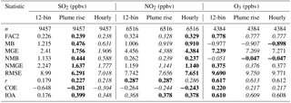
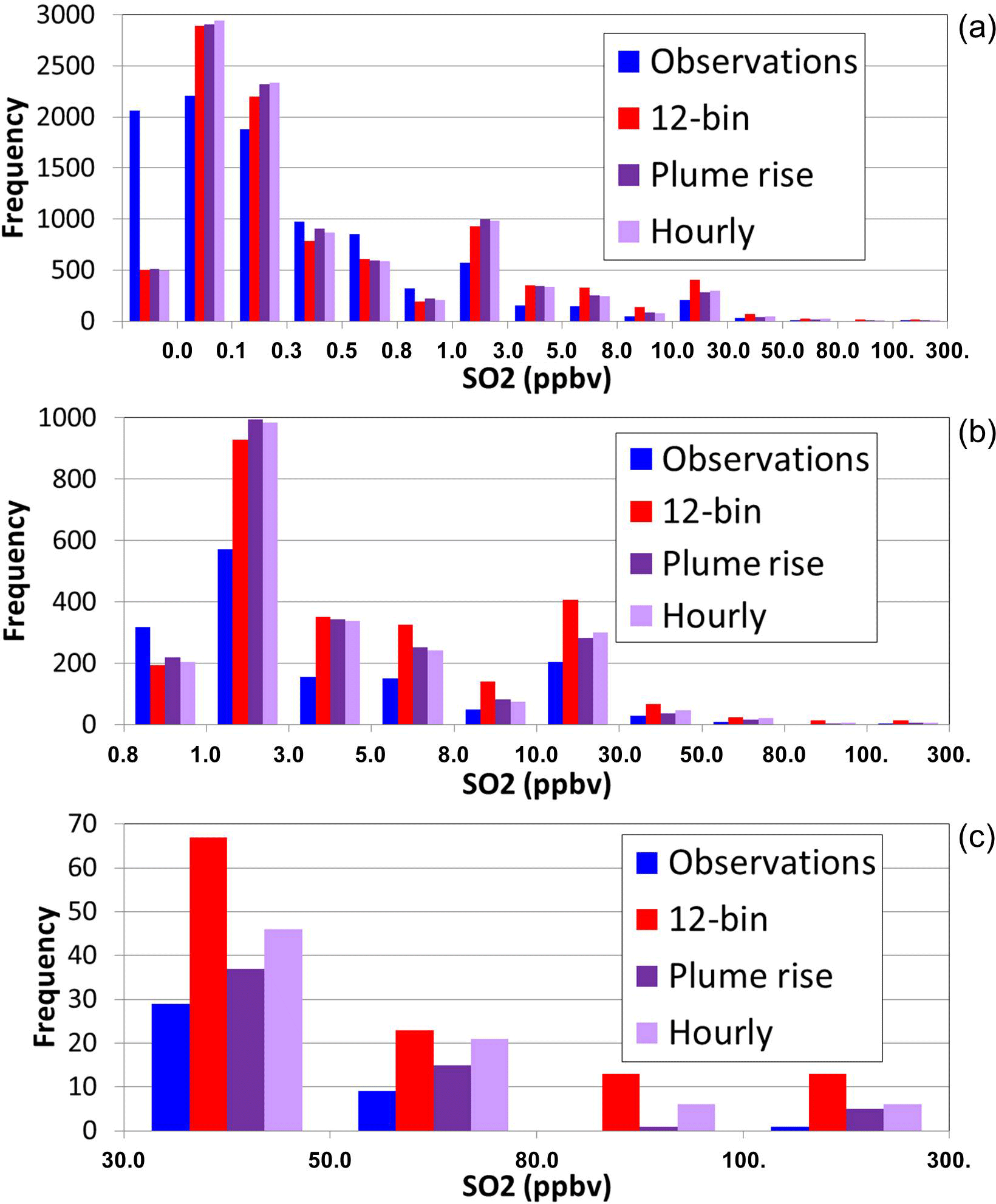
Figure 4Histograms of hourly surface SO2 mixing ratios, in logarithmic mixing ratio bins, observations (blue), original plume-rise algorithm (red), revised plume-rise algorithm (dark purple), revised plume-rise algorithm driven by hourly CEMS stack data (light purple). (a) All values; (b) 0.8 to 300 ppbv; (c) 30 to 300 ppbv.
The performance of the three model simulations using different plume-rise algorithms, for surface mixing ratios of SO2 observed at WBEA stations, is shown in Fig. 4. The model simulations are biased low for zero concentration levels (first bin, Fig. 4a), are biased high from 0.0 to 0.3 ppbv, biased low from 0.3 to 1.0 ppbv (Fig. 4a), and biased high for all concentrations above 1 ppbv (Fig. 4b, c). These last two ranges (Fig. 4b, c) result from surface fumigation of high-concentration plumes in the region studied. While all model simulations are biased high for these fumigating plumes, the plume rise and hourly simulations have a reduced bias compared to the original 12-bin plume-rise algorithm. The use of the hourly stack parameters derived from continuous emissions monitoring (hourly) has somewhat worse performance than the same plume-rise algorithm driven by annual reported stack parameters (plume rise).
The SO2 statistics of Table 5 show sometimes substantial improvements in model performance with the use of the revised plume-rise algorithms, with the mean bias being reduced by 61 %, the mean gross error by 27 %, the correlation coefficient increasing by 26 %, and the index of agreement increasing by a factor of 2.26 between the 12-bin and plume-rise algorithms, and the second best score (italics) out of the three simulations being the hourly simulation employing the revised volume flow rates and stack temperatures. For NO2, the hourly values (employing the hourly volume flow rates and temperatures) tend to have the best scores, though the differences between hourly and plume-rise simulations, where the only difference in the plume treatment is in the source of data for the initial buoyancy flux, are relatively small. Both of the primary pollutants have shown a noticeable improvement in performance with the new plume-rise treatment, with the pollutant for which most emissions are from stacks (SO2) having the most noticeable changes.
Table 6Comparison of statistical measures of SO2, NO2, and O3 measurements from the aircraft campaign against the 2.5 km resolution GEM-MACH simulations between 13 August and 10 September 2013.
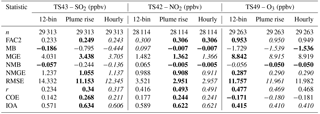
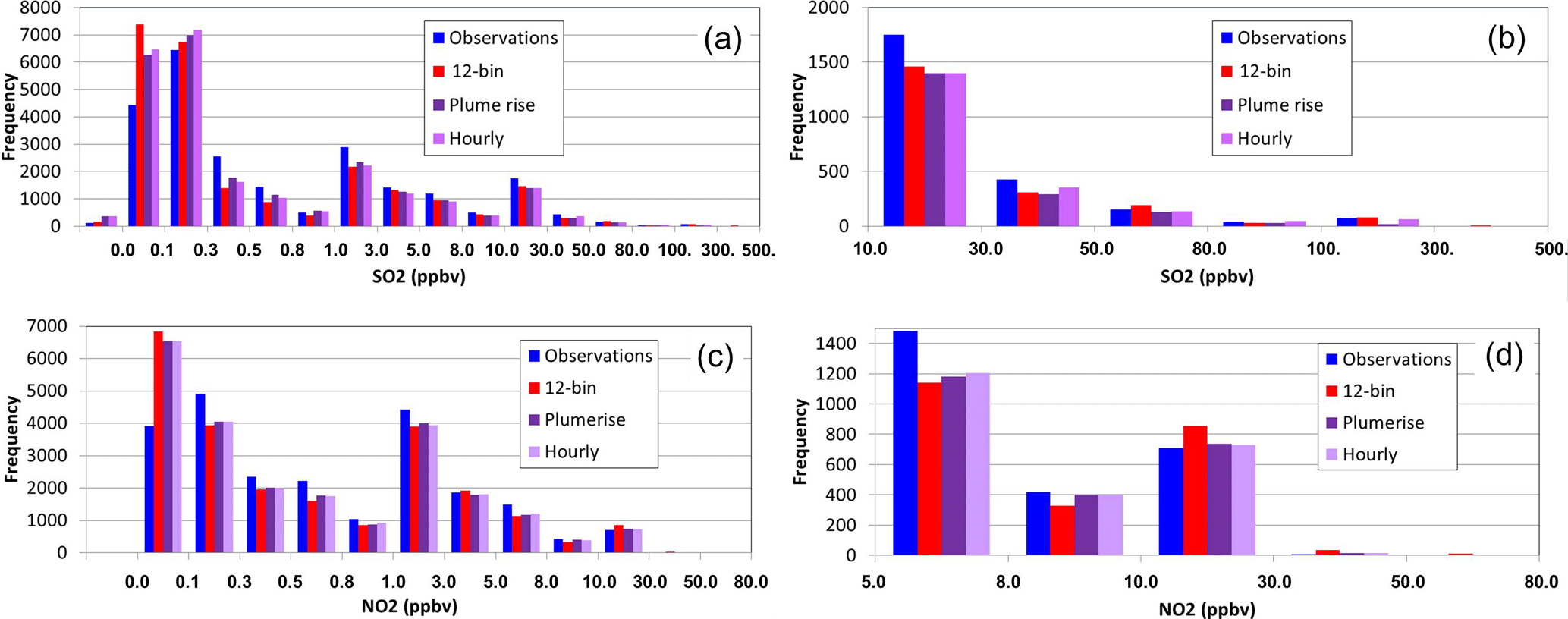
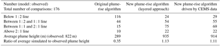
Figure 5Histograms comparing SO2 and NO2 simulations mixing ratios (ppbv) with aircraft observations. (a) All SO2 values. (b) Higher SO2 mixing ratios. (c) All NO2 values. (d) Higher NO2 mixing ratios. Leftmost histogram bin in panels (a) and (c) correspond to values of zero.
Ozone, in contrast, is created or destroyed through secondary chemistry over relatively longer time spans than the transport time from the sources in this comparison (spatial scales on the order of tens of kilometres). Accordingly, the impact of the plume rise of NOx on ozone formation is relatively minor, usually in the third decimal place (though first decimal place improvements occur for the mean bias with the use of the new plume-rise algorithm).
Overall, these results suggest that the revised plume-rise algorithm improves the model surface performance for primary pollutants largely emitted from stack sources (SO2) or for which a large proportion of the emitted mass is via stack sources (NO2). Also, the impact of the hourly volume flow rates and temperatures versus typical annual values is relatively small, though it results in a degradation of performance.
Statistical comparisons of model results computed against aircraft observations for SO2, NO2, and O3 for all the flights in the aircraft campaign are shown in the Table 6. Histograms of model performance for SO2 aloft are shown in Fig. 5. With the exception of more negative biases, the two sets of atmospheric SO2 concentrations calculated by the new plume-rise algorithm driven using annual reported stack parameters again give the best results when compared to the aircraft measurements, for all statistical measures aside from the biases (the plume-rise and hourly simulations are biased lower than the 12-bin simulation). The variations in the statistical performance between different plume-rise algorithms aloft are larger than those noted above for the surface observation comparisons, for the model scenario with plume-rise and hourly scenarios, with the former having the best overall performance. A more substantial improvement for NO2 with the revised plume-rise algorithm may be seen in comparison to the surface observation evaluation, with larger decreases in the mean bias, mean gross error, and root mean square error, and increases in the scores for correlation coefficient, coefficient of error, and index of agreement, between the 12-bin and plume-rise simulations. The results for the two simulations using the new plume-rise algorithm however remain similar for NO2. It should be noted as well that the model generally performs better against the aircraft measurements than the comparisons to the surface observations across all the statistical measures for NO2, reflecting the aircraft sampling a greater proportion of NO2 mass originating from elevated plumes as opposed to surface sources. Similar to the surface observation comparisons, the atmospheric O3 concentration calculated by the various model scenarios shows very minimal variation in the comparative statistics with the aircraft observation, with the exception of a marginally better correlation coefficient (r=0.477) for original plume-rise scenario compared to the result (r=0.6947) for the new plume-rise scenarios.
Figure 5 shows the histograms comparing aircraft observations with the results of the three variations of plume-rise algorithms for SO2 (Fig. 5a, b) and NO2 (Fig. 5c, d). In contrast to Fig. 4, all model simulations for SO2 aloft are biased low between mixing ratios of 0.3 and 50 ppbv and remain biased low above 50 ppbv for the plume-rise and hourly simulations. Thus, model estimates of surface SO2 mixing ratios (Fig. 3) are biased high, while aloft (Fig. 5a, b) SO2 mixing ratios are biased low. A similar, though less pronounced, pattern may be seen for NO2 (Fig. 5c, d), with model mixing ratios aloft biased low for histogram bins between 0.1 and 10 ppbv. All versions of the model thus have a tendency to underpredict the height of the plumes, overestimating surface fumigation events and underestimating occurrences when the plume remains aloft.
The results across the different simulations suggest that the overall model performance may be hampered by a tendency to place too much emitted mass close to the surface and insufficient mass aloft. In order to determine possible causes for this behaviour, we carried out several additional analyses.
First, we examined the 12th flight of the observation study, which took place between 16:30 and 20:30 UTC (10:30 to 14:30 local time) on 24 August, as a case study to show the differences between the three simulations examining the impacts of the choice of plume-rise algorithm and its input parameters. Flight 12 was an emissions flight, with the aircraft flying around the boundary of a single facility (Syncrude), with elevations gradually increasing in two successive sets of passes around the boundary. Data collected during flights of this nature were used to estimate emissions from the facility via calculation of the fluxes into and out of the facility from the collected data (Gordon et al., 2015). During flight 12, the aircraft carried out two successive sequences circling the facility boundaries in gradual upward spirals (between 17:00 to 18:15 and 18:45 to 19:45 UTC), starting at the lowest aircraft altitude above the surface and gradually increasing in elevation on each pass around the facility. The SO2 plume was thus intersected at multiple times and multiple heights during each of these periods. Figure 6a, b, and c depict the model-derived SO2 mixing ratio profiles at 10 s intervals interpolated from the aircraft positions as a function of time, as mixing ratio contours, for the 12-bin, plume-rise, and hourly scenarios, respectively. The aircraft locations are shown as coloured dots over-plotted on the background model mixing ratio contours. Each high mixing ratio spike in the panels of Fig. 6 thus represents a successive pass through the model SO2 plume – the change in these plumes as a function of time may be seen by following the changes in the plume cross sections in each panel along the x-axis timeline, from left to right. Between 17:00 and 18:15 UTC, the simulated plumes are mostly aloft. The 12-bin simulation employing the original Briggs algorithm (Fig. 6a) begins to fumigate significantly by 17:30 UTC, with higher concentrations reaching the surface, while for the plume-rise simulation (Fig. 6b) the plume both reaches higher elevations and experiences significantly less fumigation. The hourly simulation (Fig. 6c) is intermediate between the other two simulations. In the second period (18:45 to 19:45 UTC), the fumigation behaviour becomes more pronounced for all three simulations and once again is strongest for the 12-bin simulation (Fig. 6a), weakest for the plume-rise simulation (Fig. 6b), and intermediate for the hourly simulation (Fig. 6c).

Figure 6Model SO2 profile along the aircraft path for flight 12: (a) 12-bin simulation (original plume-rise algorithm), (b) plume-rise simulation (revised plume-rise algorithm), and (c) hourly simulation (revised plume-rise algorithm combined with hourly data for volume flow rates and stack temperatures). Panels (a–c) show model predictions in the column of the aircraft trajectory as concentration contours – aircraft-observed values at the aircraft locations at the given time (in UTC) – are shown as coloured dots over-plotting the background contours.
While the aircraft values are difficult to discern in Fig. 6, the collected aircraft SO2 observation data at successive plume intersections during each of the two intervals were extracted from the data record, arranged so that “first plume intersection” values were vertically aligned, and the vertical intervals between these successive aircraft passes were linearly interpolated in the vertical to yield observation-based cross sections of SO2 mixing ratios for each of the two time intervals. These are compared to the model plumes between 17:42 and 17:54 and between 19:08 and 19:20, in Fig. 7a and b, respectively. In the first interval (Fig. 7a), the observed plume (far right profile) can be seen to be completely detached from the surface, with concentrations < 3 ppbv located below a > 100 ppbv region between 460 and 520 m elevation. All three model plumes show more fumigation than the observations, with the plume-rise simulation showing the least fumigation of the three simulations and the 12-bin simulation showing the most fumigation. In the second interval (Fig. 7b), the observed plume is located significantly higher than the model plumes (the plume-rise simulation plume is the closest of the three in terms of elevation, but all three model plumes underestimate the plume height by several hundred metres). While the observed plume during this second interval shows some signs of fumigation at the lowest elevation, the observed concentrations at the lowest aircraft elevation are less than 30 ppbv, while the lowest model mixing ratios in the fumigation region are approximately 70 ppbv for the plume-rise simulation and above 100 ppbv for the other two simulations. The case study thus echoes the statistical analysis of Figs. 4 and 5: all model simulations tend to under-predict the plume top and overpredict the extent of fumigation for flight 12.

Figure 7Zoomed-view of Fig. 5. (a) 17:42–17:54 UTC: observations interpolated from successive flight passes between 17:00 and 18:19 UTC. (b) 19:08–19:20 UTC: observations interpolated from successive flight passes between 18:42 and 19:45 UTC.
While the comparison is encouraging in that both of the simulations employing the new plume-rise algorithm (Fig. 7b, c) out-perform the original (Fig. 7a) for most metrics (Fig. 6f), the use of the CEMS-observed volume flow rates and temperatures with the new algorithm result in a degradation of performance, relative to the simulation making use of annual averages for these parameters. That is, the believed-to-be-more-realistic stack parameters result in slightly worse performance, which is a cause for concern. The average of the hourly observed volume flow rates and temperatures for this facility's stack during flight 12 are 581.5 m3 s−1 and 472.69 K, respectively, while the corresponding annual reported values are 1174.5 m3 s−1 and 513.2 K. With respect to Eq. (1), the relative ratio of the buoyancy flux with these two sets of parameters will be
where the subscripts “r” and “o” indicate the annual reported and hourly observed values of each quantity. Assuming an ambient temperature at stack height of 291 K, the value of R is 2.28; that is, the initial buoyancy flux of the plume-rise simulation is over double that of the hourly simulation. The hourly values are believed to be more realistic during the period simulated (though include engineering emissions estimates during upset conditions) – the revised algorithm, while providing better results than the original, thus still has a tendency to under-predict the plume heights. In our companion paper, we found that the revised algorithm (therein referred to as the layered approach) had no significant advantages over the original Briggs algorithms – here we have found this revised approach has considerable benefit, while showing the same overall tendency to under-predict plume heights as in our companion paper.
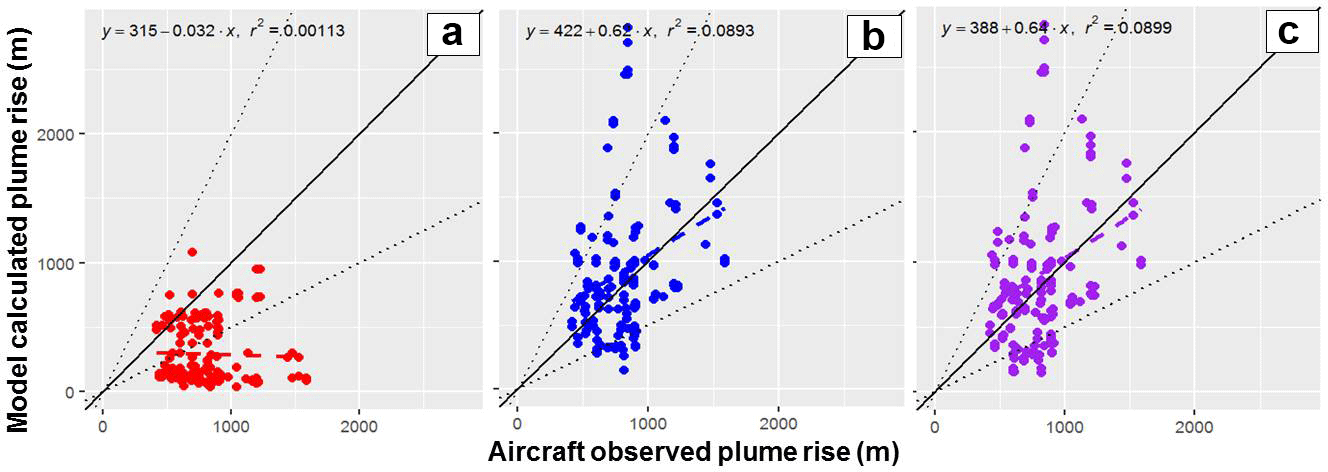
Figure 8Observed plume-rise heights during aircraft emission box flights compared to model calculated plume-rise using (a) the original plume-rise algorithm, (b) new plume-rise algorithm, and (c) new plume-rise algorithm and CEMS hourly stack temperature and volume flow rate.
In order to demonstrate the extent to which the plume-rise values themselves differ between flights, we have compared the calculated plume heights from each of the three algorithms examined here for eight stacks (located at the Syncrude, Suncor, and CNRL facilities) against observations during the course of the study (Fig. 8). The observed plume-rise values here were derived from estimates of the SO2 plume centres from the aircraft campaign's emission box flights as estimated in our companion paper (Gordon et al., 2017). Despite the differences visible in Figs. 6 and 7, for flight 12, Fig. 8 shows that the revised algorithm has a significant impact on calculated plume heights, greatly increasing the number falling within a factor of 2 of the observations, while the original algorithm has the majority of calculated plume heights falling below the 1 : 1 line, in accord with Gordon et al. (2017). However, the impact of the differences in volume flow rates and temperatures (Fig. 8b versus Fig. 8c) is usually relatively minor, with the exception of a few additional points falling below the 1 : 2 line for the hourly (Fig. 8c) simulation. Table 7 shows the relative distribution of the 176 test cases compared in terms of their distribution about the 1 : 2, 1 : 1, and 2 : 1 lines of the scatter plots of Fig. 8. The revised plume-rise approach results in a significant improvement in the distribution, and the use of CEMS data results in a slight further improvement in the average predicted plume height. We note that the relatively small differences between Fig. 8b and c, and between the last two columns of Table 7, imply that the residual buoyancy approach of Eq. (9) was relatively insensitive to the range of the initial buoyancy flux resulting from the two sets of emissions data used here, compared to the temperature gradients in Eq. (5). The large deviation between the annual reported and measured stack parameters for flight 12 may thus be an anomaly relative to the entire record across all eight stacks examined here. Nevertheless, Figs. 4 to 7 suggest that all of model simulations have a tendency to overestimate fumigation, so we continued our examination using flight 12 as a case study.
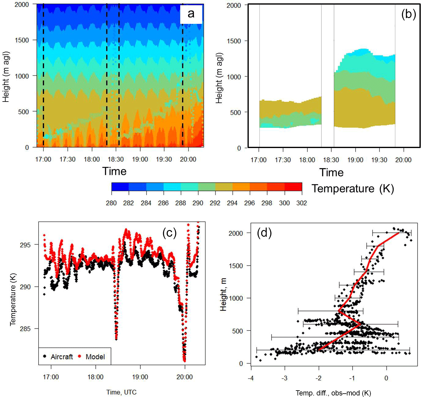
Figure 9Model versus observed temperatures, flight 12. (a) Background model-predicted temperature profiles with observed temperatures overlaid (dots) with the same colour scale. (b) Observed temperatures along the portion of the transect containing the plumes, between 17:00 and 18:18 and between 18:32 and 19:45 UTC. (c) Model (red) and observed (black) temperatures as a function of time; (d) temperature deviation (observations – model) as a function of height, with the red line showing the mean deviation at every 100 m.
The model concentrations of primary pollutants are also modified by vertical diffusion and advection. The use of a plume-rise algorithm simultaneously with vertical diffusion implies the potential for double-counting of some proportion of the vertical mixing, in that the observation-based plume-rise algorithms de facto incorporate vertical diffusion in their estimates of plume rise, while air-quality models must apply diffusion at all model grid-squares, including those in which plume-rise algorithms have already distributed emitted mass in the vertical. If the relative impact of vertical diffusion versus buoyant plume rise is strong, this may result in excessive vertical mixing, with the model effectively double-counting the vertical diffusion component of the net rise. The potential for overestimates of model diffusivity magnitudes resulting in excessive vertical mixing to the ground was investigated by carrying out a sensitivity run for flight 12 in which diffusivities in the column were halved prior to their use in calculating vertical diffusion. This sensitivity run showed a minimal impact on model results – the magnitude alone of vertical diffusion did not influence the fumigation noted below. However, this test did not examine the potential changes associated with different magnitude changes in diffusivity as a function of height.
All of the plume-rise algorithms are limited by the accuracy of the online model to accurately predict the meteorological quantities required in Eqs. (1) through (9). We note that the original Briggs algorithms (Eqs. 1 through 8) are more strongly dependent on the model's ability to accurately predict meteorological conditions close to the surface, at stack height, as well as bulk parameters such as the Obukhov length, while the revised algorithm (Eqs. 1, 5, and 9) are more strongly dependent on the model's ability to accurately predict the temperature profile throughout the column.
We examined the model's temperature predictions and compare them to observations aboard the aircraft in Fig. 9. Figure 9a shows the model-predicted temperatures in the columns around the Syncrude facility as colour contours in height versus time, similar to the mixing ratio cross sections of Fig. 6. The corresponding aircraft temperatures are over-plotted on Fig. 9a as coloured dots employing the same temperature scale as the model values. The aircraft values, particularly in the first of the two emissions spiral periods (bracketed by vertical dashed lines in Fig. 9), suggest that the model temperatures are biased high in the lowest part of the atmosphere. Fig. 9b shows the temperature cross sections interpolated from aircraft observations collected during the portion of the aircraft flight track crossing the SO2 plume to represent the average temperature profiles in each of the two regions. The first of these two cross sections shows an observed temperature inversion at the lowest aircraft altitudes, absent in the model temperature profile. In the second profile of Fig. 9b, the inversion is no longer apparent. The model-predicted temperatures in the lowest part of the atmosphere are also biased high relative to both observation-based temperature cross sections (compare Fig. 9b, which corresponds to the dashed-line bordered regions of Fig. 9a). Figure 9c and d show the variation between model and observed temperatures in two other ways: as a pair of temperature time series during the model flight (Fig. 9c) and as a scatter plot showing the differences in temperature (observed – model) as a function of height (Fig. 9d).
All of these temperature comparisons suggest that, for flight 12, the model tended to have positive temperature biases near the surface – biases which gradually decreased with height (Fig. 9d). The model atmosphere would thus be expected to be less stable than the observed atmosphere, with temperature gradients reduced in magnitude relative to observations. The model also reported positive values of the Obukhov length during the period (neutral to stable atmospheres; the Briggs formula employed would be Eqs. 3 or 4), while the smaller magnitude temperature gradients in the model drives parameter s (Eq. 5) to smaller values. While s features in the stable atmosphere formula (3), it does not feature in the neutral atmosphere formula. That is, the original Briggs formulae are relatively insensitive to errors in the temperature profile in near-neutral conditions, with only a weak influence via the Fb term. However, the revised algorithms (Eqs. 9, 1, and 5) will be influenced by the accuracy of the temperature gradient at every point throughout the temperature profile. This analysis suggests that the original Briggs algorithms (the 12-bin simulations) will be less influenced by the temperature errors shown in Fig. 9d, while the revised approach (plume rise and hourly) will be more influenced by them, contributing to higher estimates of plume heights.
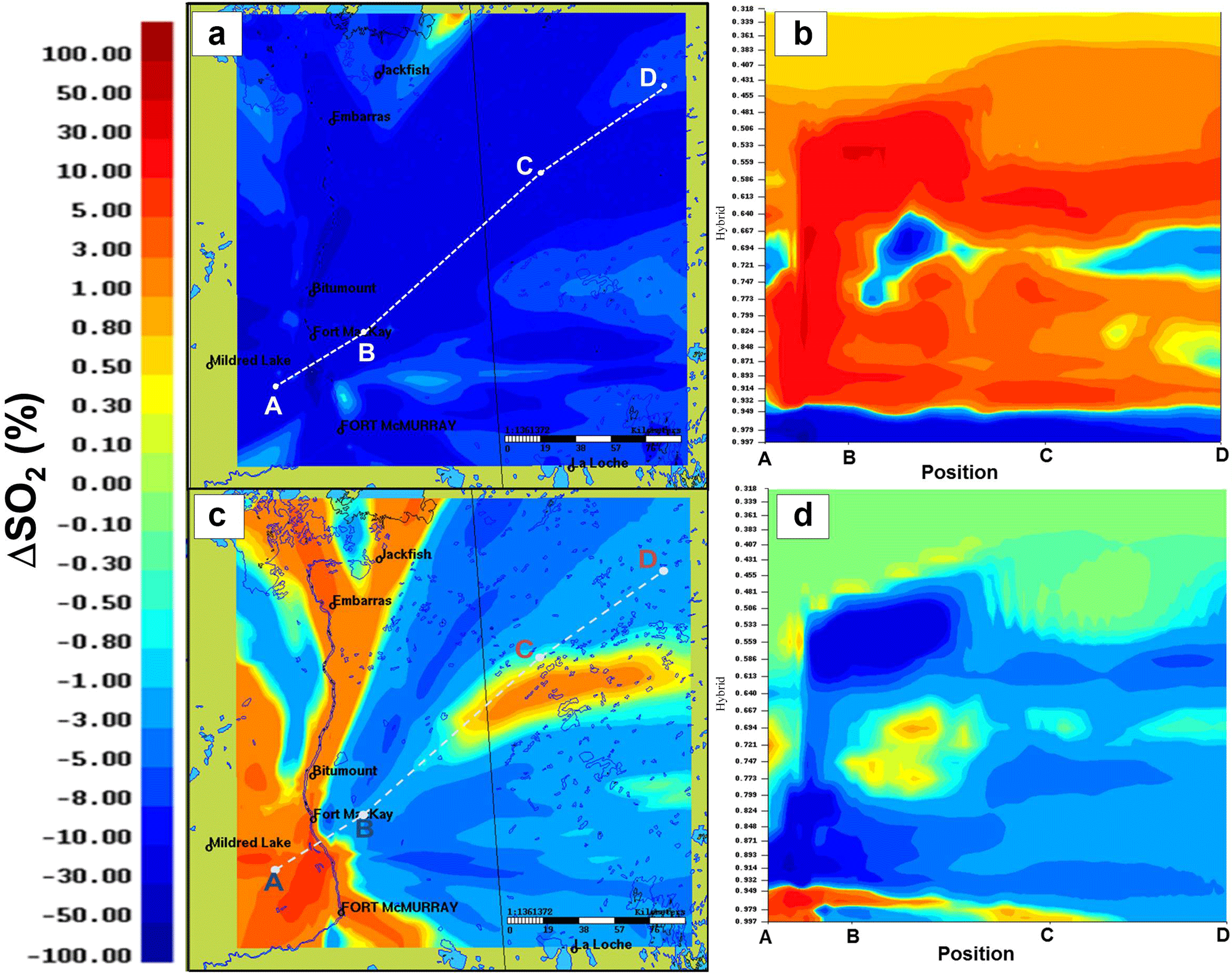
Figure 10Comparison of model-generated average mixing ratios: percent differences in multi-week averages. (a) Average surface mixing ratio percent differences for plume rise–12-bin. (b) Average cross-section percent differences along cross-section A → B → C → D for plume rise–12-bin. (c) Average surface mixing ratio percent differences for hourly–plume rise. (d) Average cross-section percent differences along cross-section A → B → C → D for hourly–plume rise.
This particular case study thus places an important caveat on our results – while the revised plume-rise approach provides better results and a better estimate of plume rise relative to the observations, it may be doing so in part in response to a model overestimate of surface heating and the corresponding reduction in the magnitude of the temperature gradient, to which the latter algorithm is sensitive and to which the original Briggs algorithms are less sensitive.
Our final analysis examines the effects of the different plume-rise algorithms on the broader region through comparisons of multi-week average differences of surface and downwind vertical cross-section mixing ratios of SO2 (Fig. 10). The change in SO2 (plume rise − 12-bin) average surface mixing ratio and a representative cross section are shown in Fig. 10a and b, while the corresponding differences for the two simulations employing the revised algorithm (hourly − plume rise) are shown in Fig. 10c, d. The first comparison (Fig. 10a) shows the substantial impact of the revised plume-rise algorithm relative to the original Briggs formulation; surface concentrations of SO2 have decreased over most of the domain, by up to 50 %. The corresponding cross section (Fig. 10b) shows that most of the SO2 removed from the surface is transported aloft, resulting in substantial relative increases in SO2 mixing ratios throughout the lower troposphere. The second comparison (Fig. 10c, d) shows that the use of hourly CEMS stack parameter data results in substantial local increases and decreases – changes in plume height associated with the use of the hourly stack parameters are sometimes responsible for both positive and negative changes between +50 and −50 %, relative to the simulation driven by annual reported stack parameters. The SO2 mass formerly being carried aloft now fumigates downwind in the hourly cross section.
In similar evaluations for NO2 (not shown), percentage differences of up to 10 % in NO2 surface mixing ratio and less than 1 % maximum difference in surface ozone mixing ratio for the 30-day average period were found. The choice of a plume-rise algorithm thus has a substantial impact on average surface and lower troposphere concentrations of those species predominantly emitted from large stacks.
We have carried out a set of four model scenarios for a 2.5 km resolution nested domain using the GEM-MACH air-quality forecast model for the Athabasca oil sands region of Alberta, Canada. These scenarios have allowed us to examine the relative impacts of aerosol size distribution and plume-rise algorithms on model performance, relative to surface and aircraft observations of multiple chemical species.
While a 2-bin configuration with sub-binning of microphysical processes has been employed in the past for operational forecasting due to computational processing time constraints (Moran et al., 2010), we find that the 12-bin configuration has better performance for all surface PM2.5 prediction metrics, including an overall 34 % reduction in the magnitude of the bias of PM2.5, for a 25 % increase in processing time.
Comparisons with the model and observed stack plumes showed that all algorithms tended to under-predict plume heights, in accord with our companion measurement-driven investigation of plume rise using the Briggs (1984) plume-rise algorithm (Gordon et al., 2017). However, in contrast to that work, significant improvements to model performance were found with the adoption of a revised plume-rise algorithm, also based on Briggs (1984), in which local changes in stability in individual model stable and neutral model layers are used to calculate the fractional reduction in buoyancy of the rising plume. Tests of the revised algorithm using annually reported stack parameters and hourly parameters from a combination of continuous emissions monitoring and engineering estimates both resulted in significant improvements in model performance in comparison to the original approach. However, the latter approach was also shown to be relatively insensitive to the range of initial buoyancy fluxes resulting from the two different emissions estimates, with the use of hourly observed (and presumed more accurate) stack parameters resulting in a slight degradation of performance relative to the use of annual reported values for these parameters. Further investigation using a specific case study suggested that the improvements associated with the revised algorithm may in part be due to model positive biases in lower atmospheric temperature, resulting in model underestimates in the magnitude of atmospheric temperature gradients. Nevertheless, the revised approach was found to correct much of the predominantly negative bias in predicted plume height seen for Briggs' original algorithms, correcting the biases in plume height noted in our companion paper, in which the algorithms were driven using observed meteorology.
Despite these improvements, and the tendency of the model to underestimate temperature gradients, the model still over-predicts the extent of fumigation for all plume-rise algorithms tested, implying the need for further work. The revised approach found to be the most favourable in the current work is based on two key parameters – entrainment coefficients determined by Briggs from data collected in 1975 to be approximately 0.08 and 0.4, respectively; we recommend that these coefficients be re-estimated using more recent data.
Our simulations have shown that the choice of a plume-rise parameterization has a very significant impact on downwind concentrations of SO2 from the oil sands sources, with the approaches having the more accurate plume heights also resulting in significant reductions in surface SO2 and increases in SO2 aloft, helping to correct pre-existing positive and negative biases in the model at these elevations. Smaller impacts were found for NO2, and minimal impacts were found for ozone.
The aircraft observations used in this study are publicly available on the ECCC data portal (ECCC, 2018). The hourly surface monitoring network data are from the public website of the Wood Buffalo Environmental Monitoring Association (WBEA, 2018). The model results are available upon request to Ayodeji Akingunola (ayodeji.akingunola@canada.ca). GEM-MACH, the atmospheric chemistry library for the GEM numerical atmospheric model (©2007–2013, Air Quality Research Division and National Prediction Operations Division, Environment and Climate Change Canada), is a free software which can be redistributed and/or modified under the terms of the GNU Lesser General Public License as published by the Free Software Foundation – either version 2.1 of the license or any later version. The specific GEM-MACH version used in this work may be obtained on request to ayodeji.akingunola@canada.ca. Much of the emissions data used in our model are available online: Executive Summary, Joint Oil Sands Monitoring Program Emissions Inventory report (JOSM, 2016a, b); and Joint Oil Sands Emissions Inventory Database (JOSM, 2018). More recent updates may be obtained by contacting Junhua Zhang or Michael D. Moran (junhua.zhang@canada.ca, mike.moran@canada.ca).
AA and PAM were responsible for the study design and methodology, model simulations, comparison to observations, and the writing of the manuscript and modifications of the same. JZ, MDM, and QZ contributed emissions data used in the modelling. AD and SML contributed aircraft observation data used for model evaluation. MG contributed aircraft plume height analyses, contributed information on the companion paper, and contributed to the text and revisions of the manuscript.
The authors declare that they have no conflict of interest.
This article is part of the special issue “Atmospheric emissions from oil sands development and their transport, transformation and deposition (ACP/AMT inter-journal SI)”. It is not associated with a conference.
This project was jointly supported by the Climate Change and Air Quality
Program of Environment and Climate Change Canada, Alberta Environment and
Parks, and the Oil Sands Monitoring program. The figures in this work were
created using a combination of Environment Canada and Climate Change software
and the openair graphics package (Carslaw and Ropkins, 2012).
Edited by: Randall Martin
Reviewed by: two anonymous referees
Ashrafi, K., Orkomi, A. A., and Motlagh, M. S.: Direct effect of atmospheric turbulence on plume rise in a neutral atmosphere, Atmos. Pollut. Res., 8 640–651, 2017.
Belair, S., Crevier, L.-P., Mailhot, J., Bilodeau, B., and Delage, Y.: Operational implementation of the ISBA land surface scheme in the Canadian regional weather forecast model, J. Hydrometeorol., 4, 352–370, 2003a.
Belair, S., Brown, R., Mailhot, J., Bilodeau, B., and Crevier, L.-P.: Operational implementation of the ISBA land surface scheme in the Canadian regional weather forecast model. Part II: cold season results, J. Hydrometeorol., 4, 371–386, 2003b.
Bieser, J., Aulinger, A., Matthias, V., Quante, M., and Denier van der Gon, H. A. C.: Vertical emission profiles for Europe based on plume rise calculations, Environ. Pollut., 159, 2935–2946. https://doi.org/10.1016/j.envpol.2011.04.030, 2011.
Briggs, G. A.: Plume rise. Report for U.S. Atomic Energy Commission, Critical Review Series, Technical Information Division report TID-25075, National Technical Information Service, Oak Ridge, Tennessee, USA, 1969.
Briggs, G. A.: Plume rise predictions, Lectures on air Pollution and environmental impact analyses, in: Workshop Proceedings, 29 September–3 October, American Meteorological Society, Boston, MA, USA, 59–111, 1975.
Briggs, G. A.: Plume rise and buoyancy effects, atmospheric sciences and power production, in: DOE/TIC-27601 (DE84005177), edited by: Randerson, D., TN, Technical Information Center, U.S. Dept. of Energy, Oak Ridge, USA, 327–366, 1984.
Byun, D. W. and Ching, J. K. S.: Science algorithms of the EPA Models-3 community multiscale air quality (CMAQ) modeling system, US EPA, Office of Research and development, EPA/600/R-99/030, Washington, D.C., USA, 1999.
Byun, D. W. and Schere, K. L.: Review of the governing equations, computational algorithms, and other components of the Model-3 Community Multiscale Air Quality (CMAQ) Modeling System, Appl. Mech. Rev., 59, 51–77, https://doi.org/10.1115/1.2128636, 2006.
Caron, J.-F. and Anselmo, D.: Regional Deterministic Prediction System (RDPS) Technical Note, Environment Canada, Dorval, Quebec, Canada, 40 pp., available at: http://collaboration.cmc.ec.gc.ca/cmc/cmoi/product_guide/docs/lib/technote_rdps-400_20141118_e.pdf (last access: 15 June 2018), 2014.
Carslaw, D. C. and Ropkins, K.: openair – an R package for air quality data analysis, Environ. Modell. Softw., 27–28, 52–61, 2012.
Charron, M., Polavarapu, S., Buehner, M., Vaillancourt, P. A., Charette, C., Roch, M., Morneau, J., Garand, L., Aparicio, J. M., MacPherson, S., Pellerin, S., St-James, J., and Heilliette, S.: The Stratospheric Extension of the Canadian Global Deterministic Medium-Range Weather Forecasting System and Its Impact on Tropospheric Forecasts, Mon. Weather Rev., 140, 1924–1944, https://doi.org/10.1175/MWR-D-11-00097.1, 2012.
CMAS: https://www.cmascenter.org/smoke/, last access: 15 June 2018.
Coats, C. J.: High-performance algorithms in the sparse matrix operator kernel emissions (SMOKE) modeling system, Proceedings of the Ninth AMS Joint Conference on Applications of Air Pollution Meteorology with AWMA, 28 January–2 February 1996, Atlanta, GA, USA, American Meteorological Society, 584–588, 1996.
Côté, J., Gravel, S., Méthot, A., Patoine, A., Roch, M., and Staniforth, A.: The operational CMC/MRB global environmental multiscale (GEM) model. Part 1: design considerations and formulation, Mon. Weather Rev., 126, 1373–1395, 1998a.
Côté, J., Desmarais, J.-G., Gravel, S., Méthot, A., Patoine, A., Roch, M., and Staniforth, A.: The operational CMC-MRB global environment multiscale (GEM) model. Part II: results, Mon. Weathre Rev., 126, 1397–1418, 1998b.
ECCC: Monitoring air quality in Alberta oil sands, Environment and Climate Change Canada, available at: https://www.canada.ca/en/environment-climate-change/services/oil-sands-monitoring/monitoring-air-quality-alberta-oil-sands.html, last access: 15 June 2018.
Emery C., Jung, K., and Yarwood, G.: Implementation of an Alternative Plume Rise Methodology in CAMx. Final Report, Work Order No. 582-7-84005-FY10-20, Environ International Corporation, Austin, Texas, USA, 41 pp., 2010.
Emmons, L. K., Walters, S., Hess, P. G., Lamarque, J.-F., Pfister, G. G., Fillmore, D., Granier, C., Guenther, A., Kinnison, D., Laepple, T., Orlando, J., Tie, X., Tyndall, G., Wiedinmyer, C., Baughcum, S. L., and Kloster, S.: Description and evaluation of the Model for Ozone and Related chemical Tracers, version 4 (MOZART-4), Geosci. Model Dev., 3, 43–67, https://doi.org/10.5194/gmd-3-43-2010, 2010.
England, W. G., Teuscher, L. H., and Synder, R. B.: A measurement program to determine plume configurations at the Beaver Gas Turbine Facility, Port Westward, Oregon, J. Air. Poll. Contr. Assoc., 26, 986–989, 1976.
EPA: Plain English Guide to the Part 75 Rule, available at: https://www.epa.gov/sites/production/files/2015-05/documents/plain_english_guide_to_the_part_75_rule.pdf (last access: 15 June 2018), 2015.
EPA: EMC: Continuous Emission Monitoring Systems, available at: https://www.epa.gov/emc/emc-continuous-emission-monitoring-systems, last access: 1 February 2018.
Erbrink, H. J.: Plume rise in different atmospheres: A practical scheme and some comparisons with LIDAR measurements, Atmos. Environ., 28, 3625–3636, 1994.
Gielbel, J.: Messungen der Abgasfahnenüberhöhung eines Steinkohlekraftwerkes mit Hilfe von LIDAR (Plume Rise measurements of a pit coal power plant by means of LIDAR). Schriftenreihe der Landesanstalt fur Immissionsschutz des Landes NRW, Essen, Germany, Heft 47, pp. 42/59, 1979 (in German).
Girard, C., Plante, A., Desgagné, M., Mctaggart-Cowan, R., Côté, J., Charron, M., Gravel, S., Lee, V., Patoine, A., Qaddouri, A., Roch, M., Spacek, L., Tanguay, M., Vaillancourt, P. A., and Zadra, A.: Staggered vertical discretization of the canadian environmental multiscale (GEM) model using a coordinate of the log-hydrostatic-pressure type, Mon. Weather Rev., 142, 1183–1196, 2014.
Gong, S. L., Barrie, L. A., and Lazare, M.: Canadian Aerosol Module (CAM): a size-segregated simulation of atmospheric aerosol processes for climate and air quality models 2. Global sea-salt aerosol and its budgets, J. Geophys. Res., 107, 4779, https://doi.org/10.1029/2001JD002004, 2003a.
Gong, S. L., Barrie, L. A., Blanchet, J.-P., von Salzen, K., Lohmann, U., Lesins, G., Spacek, L., Zhang, L. M., Girard, E., Lin, H., Leaitch, R., Leighton, H., Chylek, P., and Huang, P.: Canadian Aerosol Module: A size-segregated simulation of atmospheric aerosol processes for climate and air quality models, 1, Module development, J. Geophys. Res., 108, 4007, https://doi.org/10.1029/2001JD002002, 2003b.
Gong, W., Dastoor, A. P., Bouchet, V. S., Gong, S. L., Makar, P. A., Moran, M. D., Pabla, B., Menard, S., Crevier, L.-P., Cousineau, S., and Venkatesh, S.: Cloud processing of gases and aerosols in a regional air quality model (AURAMS), Atmos. Res., 82, 248–275, 2006.
Gordon, M., Li, S.-M., Staebler, R., Darlington, A., Hayden, K., O'Brien, J., and Wolde, M.: Determining air pollutant emission rates based on mass balance using airborne measurement data over the Alberta oil sands operations, Atmos. Meas. Tech., 8, 3745–3765, https://doi.org/10.5194/amt-8-3745-2015, 2015.
Gordon, M., Makar, P. A., Staebler, R. M., Zhang, J., Akingunola, A., Gong, W., and Li, S.-M.: A Comparison of Plume Rise Algorithms to Stack Plume Measurements in the Athabasca Oil Sands, Atmos. Chem. Phys. Discuss., https://doi.org/10.5194/acp-2017-1093, in review, 2017.
Hamilton, P. M.: Plume height measurements at Northfleet and Tilbury power stations, Atmos. Environ., 1, 379–387, 1967.
Hanna, S. R. and Paine, R. J.: Hybrid Plume Dispersion Model (HPDM) Development and Evaluation, J. Appl. Meteorol., 28, 206–224, 1988.
Holmes, N. S. and Morawska, L.: A review of dispersion modelling and its application to the dispersion of particles: An overview of different dispersion models available, Atmos. Environ., 40, 5902–5928, https://doi.org/10.1016/j.atmosenv.2006.06.003, 2006.
Im, U., Roberto Bianconi, R., Efisio Solazzo, E., Kioutsioukis, I., Badia, A., Balzarini, A., Baró, R., Bellasio, R., Brunner, D., Chemel, C., Curci, G., Flemming, J., Forkel, R., Giordano, L., Jiménez-Guerrero, P., Hirtl, M., Hodzic, A., Honzak, L., Jorba, O., Knote, C., Kuenen, J.J.P, Makar, P.A., Manders-Groot, A., Neal, L, Perez, J.L., Pirovano, G., Pouliot, G., San Jose, R., Savage, N., Schroder, W., Sokhi, R.S., Syrakov, D., Torian, A., Tuccella, P., Werhahn, J., Wolke, R., Yahya, K., Zabkar, R., Zhang, Y., Zhang, J., Hogrefe, C., and Galmarini, S.: Evaluation of operational on-line-coupled regional air quality models over Europe and North America in the context of AQMEII phase 2. Part I: Ozone, Atmos. Environ., 115, 404–420, 2015a.
Im, U., Bianconi, R., Solazzo, E., Kioutsioukis, I., Badia, A., Balzarini, A., Baró, R., Bellasio, R., Brunner, D., Chemel, C., Curci, G., van der Gon, H.D., Flemming, J., Forkel, R., Giordano, L., Jiménez-Guerrero, P., Hirtl, M., Hodzic, A., Honzak, L., Jorba, O., Knote, C., Makar, P. A., Manders-Groot, A., Neal, L., Perez, J. L., Pirovano, G., Pouliot, G., San Jose, R., Savage, N., Schroder, W., Sokhi, R. S., Syrakov, D., Torian, A., Tuccella, P., Wang, K., Werhahn, J., Wolke, R., Zabkar, R., Zhang, Y., Zhang, J., Hogrefe, C., and Galmarini, S.: Evaluation of operational on-line-coupled regional air quality models over Europe and North America in the context of AQMEII phase 2. Part II: Particulate Matter, Atmos. Environ., 115, 421–411, 2015b.
Jarvis, P. G.: The interpretation of the variations in leaf water potential and stomatal conductance found in canopies in the field, Philos. T. R. Soc. Lon. B, 273, 593–610, 1976.
Joint Oil Sands Monitoring Plan (JOSM): Integrated Monitoring Plan for the Oil Sands: Air Quality Component, 72 pp., available at: http://publications.gc.ca/site/eng/394253/publication.html (last access: 26 January 2018), 2011.
JOSM: Environment and Climate Change Canada and Alberta Environment and Parks, Executive Summary, Joint Oil Sands Monitoring Program Emissions Inventory report, available at: https://www.canada.ca/en/environment-climate-change/services/science-technology/publications/joint-oil-sands-monitoring-emissions-report.html (last access: 15 June 2018), 2016a.
JOSM: Environment and Climate Change Canada, AEMERA, and Alberta Environment and Parks, Joint Oil Sands Monitoring Program Emissions Inventory Compilation Report, available at: http://aep.alberta.ca/air/reports-data/documents/JOSM-EmissionsInventoryReport-Jun2016.pdf (last access: 15 June 2018), 2016b.
JOSM: Environment and Climate Change Canada and Alberta Environment and Parks, Joint Oil Sands Emissions Inventory Database, available at: http://ec.gc.ca/data_donnees/SSB-OSM_Air/Air/Emissions_inventory_files/, last access: 15 June 2018.
Kaasik, M. and Kimmel, V.: Validation of the improved AEROPOL model against the Copenhagen data set, Int. J. Environ. Pollut., 20, 114–120, https://doi.org/10.1504/IJEP.2003.004256, 2003.
Kain, J. S.: The Kain–Fritsch convective parameterization: an update, J. Appl. Meteorol., 43, 170–181, 2004.
Kain, J. S. and Fritsch, J. M.: A one-dimensional entraining/detraining plume model and its application in convective parameterizations, J. Atmos. Sci., 47, 2784–2802, 1990.
Levy, J. I., Spengler, J. D., Hlinka, D., Sullivan, D., and Moon, D.: Using CALPUFF to evaluate the impacts of power plant emissions in Illinois: mode sensitivity and implications, Atmos. Environ., 36, 1063–1075, 2002.
Li, J. and Barker, H. W.: A radiation algorithm with correlated k-distribution. Part I: local thermal equilibrium, J. Atmos. Sci., 62, 286–309, 2005.
Li, S.-M., Leithead, A., Moussa, S. G., Liggio, J., Moran, M. D., Wang, D., Hayden, K., Darlington, A., Gordon, M., Staebler, R., Makar, P. A., Stroud, C. A., McLaren, R., Liu, P. S. K., O'Brien, J., Mittermeier, R. L., Zhang, J., Marson, G., Cober, S. G., Wolde, M., and Wentzell, J. J. B.: Differences between measured and reported volatile organic compound emissions from oil sands facilities in Alberta, Canada, P. Natl. Acad. Sci. USA, 114, E3756–E3765, 2017.
Liggio, J., Li, S. M., Hayden, K., Taha, Y. M., Stroud, C., Darlington, A., Drollette, B. D., Gordon, M., Lee, P., Liu, P., Leithead, A., Moussa, S. G., Wang, D., O'Brien, J., Mittermeier, R. L., Brook, J. R., Lu, G., Staebler, R. M., Han, Y., Tokarek, T. W., Osthoff, H. D., Makar, P. A., Zhang, J., Plata, D. L., and Gentner, D. R.: Oil sands operations as a large source of secondary organic aerosols, Nature, 534, 91–94, https://doi.org/10.1038/nature17646, 2016.
Lurmann, F. W., Lloyd, A. C., and Atkinson, R.: A chemical mechanism for use in long range transport/acid deposition computer modeling, J. Geophys. Res., 91, 10905–10936, 1986.
Mailhot, J. and Benoit, R.: A finite-element model of the atmospheric boundary layer suitable for use with numerical weather prediction models, J. Atmos. Sci., 39, 2249–2266, 1982.
Makar, P. A., Bouchet, V. S., and Nenes, A.: Inorganic Chemistry Calculations using HETV – A Vectorized Solver for the -- system based on the ISORROPIA Algorithms, Atmos. Environ., 37, 2279–2294, 2003.
Makar, P. A., Gong, W., Milbrandt, J., Hogrefe, C., Zhang, Y., Curci, G., Zabkar, R., Im, U., Balzarini, A., Baro, R., Bianconi, R., Cheung, P., Forkel, R., Gravel, S., Hirtl, H., Honzak, L., Hou, A., Jimenz-Guerrero, P., Langer, M., Moran, M. D., Pabla, B., Perez, J. L., Pirovano, G., San Jose, R., Tuccella, P., Werhahn, J., Zhang, J., and Galmarini, S.: Feedbacks between air pollution and weather, part 1: Effects on weather, Atmos. Environ., 115, 442–469, 2015a.
Makar, P. A., Gong, W., Hogrefe, C., Zhang, Y., Curci, G., Zabkar, R., Milbrandt, J., Im, U., Balzarini, A., Baro, R., Bianconi, R., Cheung, P., Forkel, R., Gravel, S., Hirtl, H., Honzak, L., Hou, A., Jimenz-Guerrero, P., Langer, M., Moran, M. D., Pabla, B., Perez, J. L., Pirovano, G., San Jose, R., Tuccella, P., Werhahn, J., Zhang, J., and Galmarini, S.: Feedbacks between air pollution and weather, part 2: Effects on chemistry, Atmos. Environ., 115, 499–526, 2015b.
Makar, P. A., Akingunola, A., Aherne, J., Cole, A. S., Aklilu, Y.-A., Zhang, J., Wong, I., Hayden, K., Li, S.-M., Kirk, J., Scott, K., Moran, M. D., Robichaud, A., Cathcart, H., Baratzedah, P., Pabla, B., Cheung, P., Zheng, Q., and Jeffries, D. S.: Estimates of Exceedances of Critical Loads for Acidifying Deposition in Alberta and Saskatchewan, Atmos. Chem. Phys. Discuss., https://doi.org/10.5194/acp-2017-1094, in review, 2018.
Milbrandt, J. A. and Yau, M. K.: A multimoment bulk microphysics parameterization. Part I: analysis of the role of the spectral shape parameter, J. Atmos. Sci., 62, 3051–3064, 2005a.
Milbrandt, J. A. and Yau, M. K.: A multimoment bulk microphysics parameterization. Part II: a proposed three-moment closure and scheme, J. Atmos. Sci., 62, 3065–3081, 2005b.
Moran, M. D., Ménard, S., Talbot, D., Huang, P., Makar, P. A., Gong, W., Landry, H., Gravel, S., Gong, S., Crevier, L.-P., Kallaur, A., and Sassi, M.: Particulate-matter forecasting with GEM-MACH15, a new Canadian air-quality forecast model, in: Air Pollution Modelling and Its Application XX, edited by: Steyn, D. G. and Rao, S. T., Springer, Dordrecht, the Netherlands, 289–292, 2010.
Munoz-Alpizar, R., Stroud, C., Ren, S., Belair, S., Leroyer, S., Souvanlasy, V., Spacek, L., Pavlovic, R., Davignon, D., and Moran, M.: Towards an operational high-resolution air quality forecasting at ECCC, 19th EGU General Assembly, EGU2017, 23–28 April 2017, Vienna, Austria, p. 3063, 2017.
Mylona, S.: Sulphur dioxide emissions in Europe 1880–1991 and their effect on sulphur concentrations and depositions, Tellus B, 48, 662–689. https://doi.org/10.1034/j.1600-0889.1996.t01-2-00005.x, 1996.
NPRI: National Pollutant Release Inventory, available at: https://www.canada.ca/en/environment-climate-change/services/national-pollutant-release-inventory/report.html, last access: 1 February 2018.
Rittmann, B. E.: Application of two-thirds law to plume rise from industrial-sized sources, Atmos. Environ., 16, 2575–2579, 1982.
Shephard, M. W., McLinden, C. A., Cady-Pereira, K. E., Luo, M., Moussa, S. G., Leithead, A., Liggio, J., Staebler, R. M., Akingunola, A., Makar, P., Lehr, P., Zhang, J., Henze, D. K., Millet, D. B., Bash, J. O., Zhu, L., Wells, K. C., Capps, S. L., Chaliyakunnel, S., Gordon, M., Hayden, K., Brook, J. R., Wolde, M., and Li, S.-M.: Tropospheric Emission Spectrometer (TES) satellite observations of ammonia, methanol, formic acid, and carbon monoxide over the Canadian oil sands: validation and model evaluation, Atmos. Meas. Tech., 8, 5189–5211, https://doi.org/10.5194/amt-8-5189-2015, 2015.
Stroud, C. A., Makar, P. A., Zhang, J., Moran, M. D., Akingunola, A., Li, S.-M., Leithead, A., Hayden, K., and Siu, M.: Air Quality Predictions using Measurement-Derived Organic Gaseous and Particle Emissions in a Petrochemical-Dominated Region, Atmos. Chem. Phys. Discuss., https://doi.org/10.5194/acp-2018-93, in review, 2018.
Turner, D. B., Bender, L. W., Paumier, J. O., and Boone, P. F.: Evaluation Of The TUPOS Air Quality Dispersion Model Using Data From The EPRI Kincaid Field Study, Atmos. Environ., 25A, 2187–2201, 1991.
VDI: VDI, Ausbreitung von Luftverunreinigungen in der Atmosphäre; Berechnung der Abgasfahnen-überhöhung (Dispersion of air pollutants in the atmosphere; determination of plume rise) 1985-06, Kommission Reinhaltung der Luft (KRdL) im VDI und DIN, 1985 – Normenausschuss, available at: http://www.vdi.de (last access: 15 June 2018), 1985 (in German/English).
WBEA: Historical monitoring data, Wood Buffalo Environmental Monitoring Association, available at: http://www.wbea.org/network-and-data/historical-monitoring-data, last access: 15 June 2018.
Webster, H. N. and Thomson, D. J.: Validation of a Lagrangian model plume rise scheme using the Kincaid data set, Atmos. Environ., 36, 5031–5042, 2002.
Wesely, M. L.: Parameterization of surface resistances to gaseous dry deposition in regional-scale numerical models, Atmos. Environ., 23, 1293–1304, 1989.
Whaley, C. H., Makar, P. A., Shephard, M. W., Zhang, L., Zhang, J., Zheng, Q., Akingunola, A., Wentworth, G. R., Murphy, J. G., Kharol, S. K., and Cady-Pereira, K. E.: Contributions of natural and anthropogenic sources to ambient ammonia in the Athabasca Oil Sands and north-western Canada, Atmos. Chem. Phys., 18, 2011–2034, https://doi.org/10.5194/acp-18-2011-2018, 2018.
Zhang, J., Zheng, Q., Moran, M. D., Makar, P. A., Akingunola, A., Li, S.-M., Marson, G., Gordon, M., Melick, R., and Cho, S.: Emissions preparation for high-resolution air quality modelling over the Athabasca oil sands region of Alberta, Canada, 21st Intern. Emissions Inventory Conference, 13–17 April 2015, San Diego, USA, 18 pp., available at: http://www.epa.gov/ttn/chief/conference/ei21/session1/zhang_emissions.pdf (last access: 18 June 2018), 2015.
Zhang, J., Moran, M. D., Zheng, Q., Makar, P. A., Baratzadeh, P., Marson, G., Liu, P., and Li, S.-M.: Emissions Preparation and Analysis for Multiscale Air Quality Modelling over the Athabasca Oil Sands Region of Alberta, Canada, Atmos. Chem. Phys. Discuss., https://doi.org/10.5194/acp-2017-1215, in review, 2018.
Zhang, L., Gong, S., Padro, J., and Barrie, L.: A size-segregated particle dry deposition scheme for an atmospheric aerosol module, Atmos. Environ., 35, 549–560, 2001.
Zhang, L., Moran, M. D., Makar, P. A., Brook, J. R., and Gong, S.: Modelling gaseous dry deposition in AURAMS: a unified regional air-quality modelling system, Atmos. Environ., 36, 537–560, 2002.
Zhang, L., Brook, J. R., and Vet, R.: A revised parameterization for gaseous dry deposition in air-quality models, Atmos. Chem. Phys., 3, 2067–2082, https://doi.org/10.5194/acp-3-2067-2003, 2003.