We present simulations from the three models (CLaMS, WACCM and TOMCAT/SLIMCAT) for the Antarctic winter 2011. This year had a rather large ozone hole with a size within the top 10 of the last 4 decades (Klekociuk et al., 2014) and was chosen because both MIPAS and MLS data were available.

The setup of the models with respect to initialisation, boundary conditions, transport schemes and PSC formation is different, which also contributes to differences between the model results. The formulation of stratospheric chemistry, especially heterogeneous chemistry of chlorine compounds, is implemented as commonly used (Jaeglé et al., 1997) and recommended, and is comparable among the three models.

The development of HCl in polar stratospheric winter is strongly influenced by heterogeneous chlorine activation. The heterogeneous reactions that cause this typically occur below a temperature threshold of about 195 K on cold binary aerosol or on PSCs composed of either HNO₃ ∕ H₂SO₄ ∕ H₂O STS solution, water ice or crystalline NAT. An important and fast HCl sink is the heterogeneous reaction ClONO₂ + HCl → HNO₃ + Cl₂ (Solomon et al., 1986). At the beginning of winter, as temperatures drop below the threshold for heterogeneous reactions to occur, this reaction quickly depletes HCl typically until all available ClONO₂ has reacted, since HCl is usually available in large excess (Jaeglé et al., 1997). This step is therefore referred to as the “titration step”. After that, since no reaction partner is available, HCl mixing ratios would remain constant in the dark in the absence of transport or mixing processes. A further depletion of HCl is only possible if there is a reaction partner. This reaction partner first needs to be formed, and in addition to ClONO₂ it could be HOCl which would then react by the heterogeneous reaction HOCl + HCl → H₂O + Cl₂ (Solomon, 1999). The resulting geographic distribution HCl and its development over the winter is presented in Fig. 1. The figure shows maps of MLS HCl observations (Froidevaux et al., 2008) and corresponding CLaMS results on the 500 K potential temperature level for selected days in May, June and July. On 21 May, when the HCl depletion due to heterogeneous processing is first apparent, the model seems to represent the observations well. By 20 June, HCl depletion has mainly occurred at the vortex edge, where it is more distinctly pronounced in the observations. The comparison on 20 July clearly demonstrates the discrepancy between simulations and observations. The model shows HCl mixing ratios well above 1.5 ppbv in the vortex core, while the MLS observations indicate almost zero values of HCl, within the limits of the total estimated uncertainty of the data.

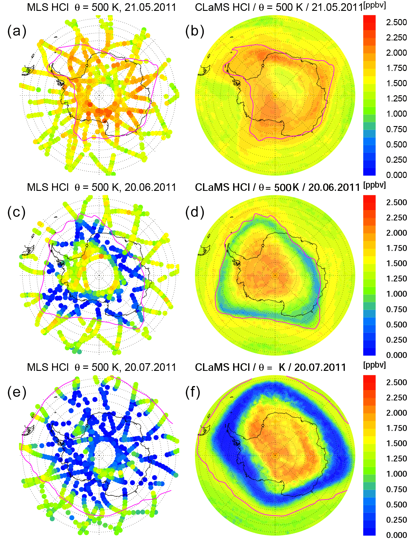
Figure 1Time series of orthographic projection of MLS observations (a, c, e) and CLaMS simulations (b, d, f)  of HCl mixing ratios on the 500 K potential temperature level. The maps are shown for 21 May (a, b), 20 June (c, d) and 20 July 2011 (e, f). The pink line depicts the edge of the polar vortex according to the criterion of Nash et al. (1996).

Download

Figure 2Depiction of MLS HCl mixing ratio data averaged in equivalent latitude/potential temperature space. Panel (a) shows the vortex-core average for equivalent latitudes poleward of 75^∘ S as a function of time and potential temperature. Panel (b) shows the time development on the 500 K potential temperature level. Panels (c, d) show a snapshot of this average on 20 June and 20 July 2011. Grey lines on the panels indicate the cuts or borders displayed in the other panels of this figure.

Download

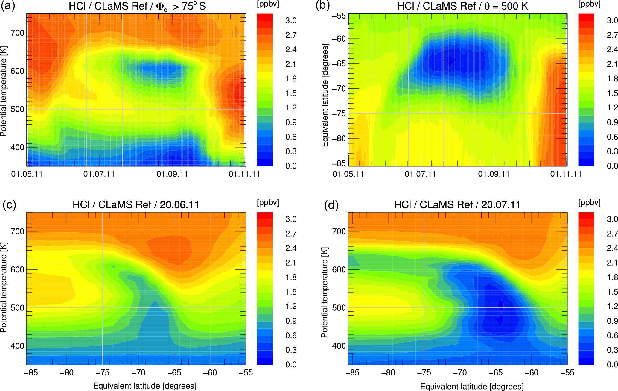
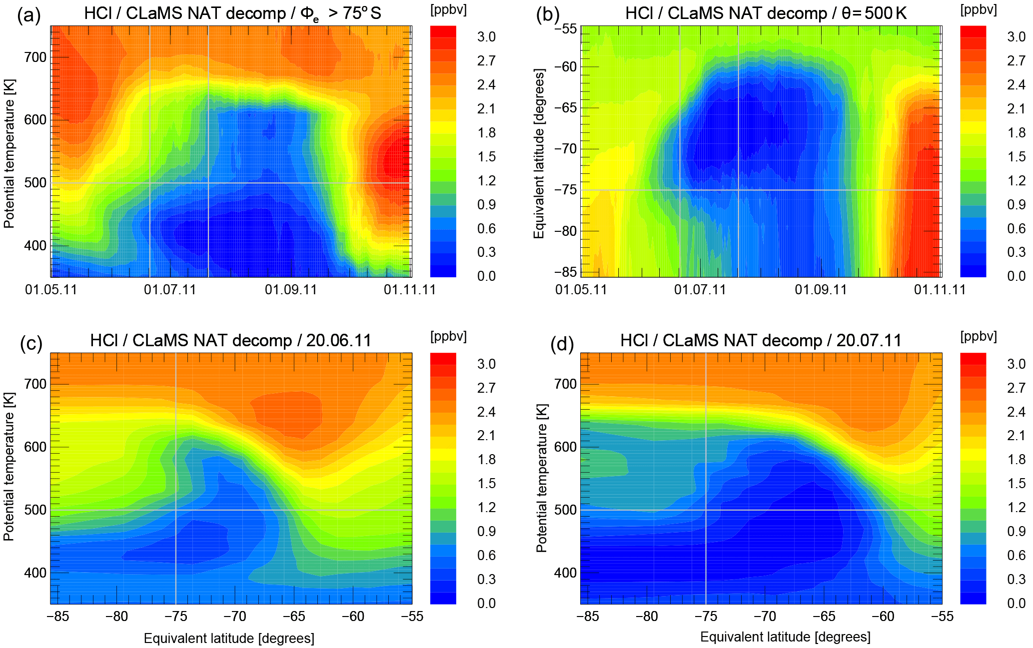
Figure 3CLaMS simulation for HCl averaged in equivalent latitude/potential temperature space displayed as in Fig. 2.

Download

To investigate the HCl discrepancy further, we averaged both the observations and simulation for each day with respect to equivalent latitude (Butchart and Remsberg, 1986) and potential temperature using 20 equivalent latitude (Φ_e) bins of equal area between Φ_e=50 and 90^∘ S. Figure 2 shows the characteristics of the observed HCl development by displaying cuts through the equivalent latitude/potential temperature space. Figure 2a shows the time development of the vortex-core average (Φ_e>75^∘ S) as a function of potential temperature. Figure 2b shows the time development on the 500 K potential temperature level. Grey lines correspond to the position of the cuts or borders displayed in the other panels. Figure 2c, d show the Φ_e ∕ θ cross sections for two selected days, 20 June and 20 July.

Figure 4Similar results as displayed in Figs. 2 and 3 for the simulation of Arctic winter 2016. Panels (a, b) depict the MLS HCl mixing ratio data averaged in equivalent latitude/potential temperature space for the vortex core (Φ_e> 75^∘ N, a) and the time development on the 475 K potential temperature level (b). Panels (c, d) show the corresponding model results from CLaMS. Grey lines on the panels indicate the cuts or borders displayed in the other panels of this figure.

Download

Figure 3 shows the corresponding results from the CLaMS simulation. The top panels of Figs. 2 and 3 agree well with respect to the time at which the HCl depletion starts at the different altitudes and latitudes. However, it appears that after the first “titration” step, HCl depletes much more slowly in the simulations compared to the MLS observations. From the comparison of Figs. 2 and 3, it is evident that the model HCl discrepancy is present over a wide altitude range throughout polar winter.

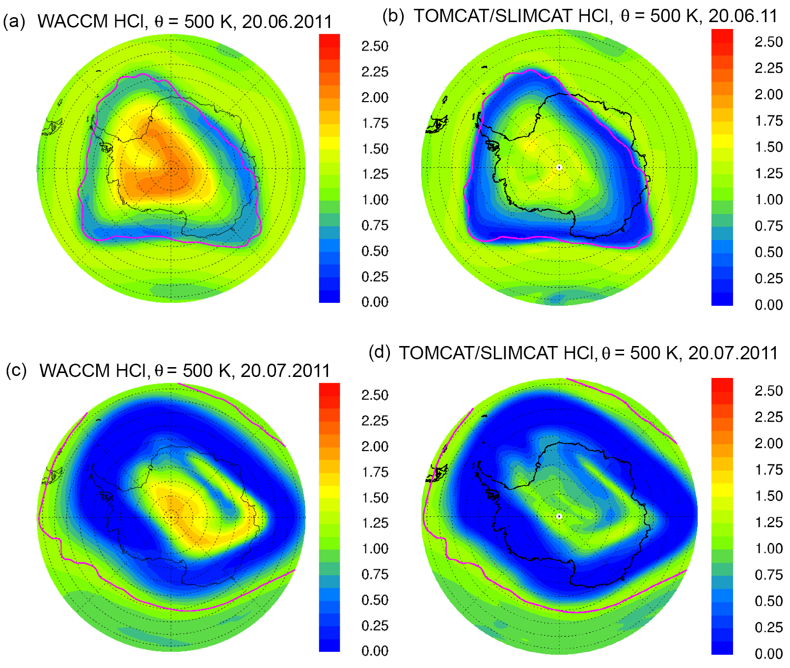
Figure 5Simulated HCl from SD-WACCM (a, c) and TOMCAT/SLIMCAT (b, d) on the 500 K potential temperature surface for 20 June (a, b) and 20 July 2011 (c, d)  displayed as in Fig. 1.

Download

Figure 4 shows the time series of the similarly averaged HCl mixing ratio for the Arctic winter 2015/2016, both for the MLS observations (Fig. 4a, b) and the CLaMS simulation (Fig. 4c, d). This winter was chosen because it was particularly cold in the stratosphere (Dörnbrack et al., 2017). Here, the HCl discrepancy is also apparent, although to a lesser extent than in the Antarctic. It is most evident at the slightly lower potential temperature of about 475 K in the Arctic vortex core. Compared with the observations, the model requires over 1 month more, until February, to reach the minimum HCl mixing ratios. While the discrepancy is therefore also present in the Arctic, in the following we focus on the Antarctic results where it is much more strongly pronounced.

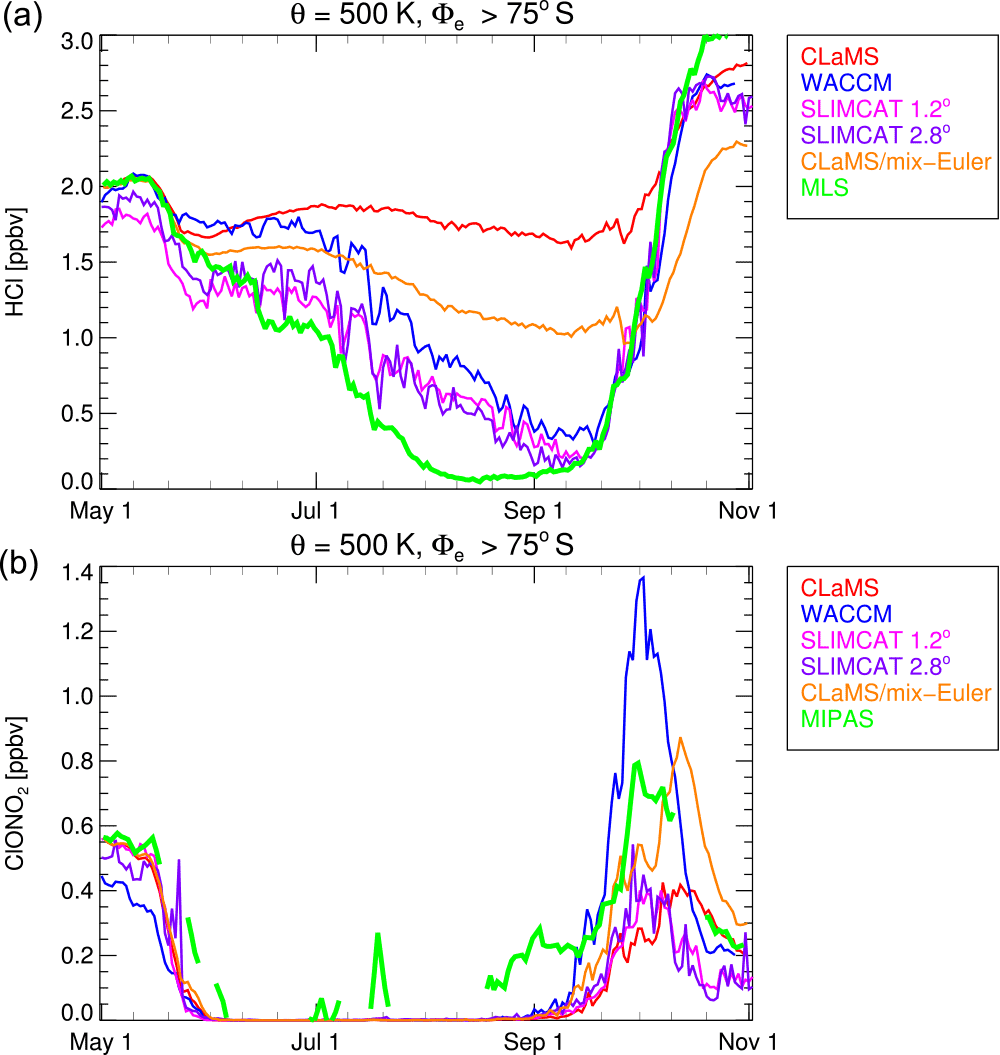
Figure 6Vortex-core averages (${\mathrm{\Phi }}_e>{\mathrm{75}}^{\circ }$S) on the 500 K isentrope for HCl (a) and ClONO₂ (b) for different model simulations. Observations of MLS and MIPAS are shown as green lines. The red line corresponds to CLaMS, the blue line corresponds to SD-WACCM, and pink and purple lines correspond to TOMCAT/SLIMCAT simulations with horizontal resolution 1.2 and 2.8^∘, respectively. The orange line corresponds to the CLaMS “mix-Euler” simulation, in which additional artificial mixing was applied.

Download

For further comparison, we now show results for the Antarctic winter 2011 simulated by the Eulerian models SD-WACCM and TOMCAT/SLIMCAT. Figure 5 shows the simulated HCl mixing ratios from these models plotted identically as in Fig. 1. The HCl discrepancy is clearly also evident in these simulations, as on 20 July, by when HCl had disappeared in the MLS data; both models also show an area of elevated HCl still present in the polar vortex core, although with lower HCl mixing ratios compared to CLaMS. The HCl depletion in the vortex core is stronger in the TOMCAT/SLIMCAT simulation than in SD-WACCM but still not comparable to the MLS observations. For a more detailed comparison, the results of SD-WACCM and TOMCAT/SLIMCAT have been averaged in Φ_e ∕ θ space in a similar manner to CLaMS and the observations. The WACCM model daily output interpolated to potential temperature levels was averaged using potential vorticity and equivalent latitude calculated from ERA-Interim data. The TOMCAT/SLIMCAT model output was directly averaged within the internal calculated equivalent latitude, also based on ERA-Interim data. A depiction corresponding to Fig. 3 but for SD-WACCM and TOMCAT/SLIMCAT is shown as Figs. S1–S3 in the Supplement. Figure 6 shows a time series of the vortex-core-average HCl and ClONO₂ simulated by the three models. The green line corresponds to the MLS and MIPAS observations for HCl and ClONO₂, respectively. However, only very limited ClONO₂ observations are available from June to August, since the presence of PSCs impedes the MIPAS retrieval process.

There are differences between the individual simulations that arise due to different model formulation and initialisation and that are discussed below. Generally, the Eulerian models SD-WACCM and TOMCAT/SLIMCAT show a faster HCl depletion than CLaMS. However, it seems that all models underestimate the rate of HCl depletion after the titration step. The three simulations presented show that the initial titration step is completed by the end of May and no further strong changes of HCl occur until early July. Differences during May are likely caused by different initial chlorine partitioning. In July and August, HCl decreases further, CLaMS being the model that indicates the slowest HCl decrease. There is even an apparent HCl increase in CLaMS that is caused by the descent of air masses with higher inorganic chlorine Cl_y.

One possible reason for the inter-model difference could be differences in the chemistry formulation of the different models. To investigate this hypothesis, box model versions of TOMCAT/SLIMCAT and CLaMS were integrated along an example trajectory. This trajectory was chosen from an ensemble of 1800 vortex trajectories of 2.5-month duration, along which the ozone and HCl development was closest to the vortex-core average shown in Fig. 6. This trajectory should therefore be representative for the vortex-core average ozone and HCl development in the 3-D model. For this example trajectory, no significant differences were found between the models. Both models similarly showed no further depletion of HCl after the titration step in the dark unmixed polar night conditions (see Fig. S4 of the Supplement). Thus, the differences among the models are unlikely due to model differences in the formulation of the chemical scheme.

A large part of the inter-model difference may be caused by the fact that the Lagrangian formulation of the model CLaMS minimises numerical diffusion while it is inherent in the Eulerian models SD-WACCM and TOMCAT/SLIMCAT. The numerical diffusion arises in Eulerian models because on each time step the chemical tracers are typically averaged within the extent of a model grid box. The minimisation of the numerical diffusion from this lower-resolution limit depends on the performance of the advection scheme; for example, the Prather (1986) scheme used in TOMCAT/SLIMCAT stores subgrid-scale distributions of the tracers. In practice, all Eulerian models likely aim to have tracer advection schemes which limit numerical diffusion, although it will always occur to some extent. The artificial mixing by numerical diffusion could provide additional ClONO₂ or HOCl as a reaction partner for HCl or NO_x that would form ClONO₂. To investigate this hypothesis, a sensitivity simulation by CLaMS was performed, in which a regular Eulerian grid with 2.8^∘ × 2.8^∘ horizontal spacing and the vertical model grid (with the vertical resolution of 800–1000 m in the lower stratosphere) as vertical levels were defined. Every 24 h of the model run it was checked whether more than one air parcel resided in the same grid box. These air parcels were then set to the average mixing ratio of all air parcels residing in the grid box. Although a Eulerian model that must average over these grid boxes on every time step would be even more diffusive, this study can at least show a lower limit of this effect. The corresponding HCl result (labelled “mix-Euler”) is shown as the orange line in Fig. 6. Indeed, the additional imposed Eulerian mixing causes a faster HCl depletion until mid-August. Although it is difficult to mimic additional numerical diffusion in a Lagrangian model, this sensitivity supports the assumption that at least part of the difference between CLaMS and the other Eulerian models may be caused by numerical diffusion. Thus, it is likely that the numerical diffusion in the Eulerian models masks part of the effect responsible for the HCl discrepancy investigated in this study. However, it should be noted there is not much difference in the development of HCl between the two resolutions of TOMCAT/SLIMCAT. In the low-resolution simulation, the gradients of ozone and other trace species, especially at the vortex edge, are weaker, but the time series of vortex-core averages are very similar. Potentially, in the high-resolution simulation, the numerical diffusion may already be significant.

In the following, we list potential model deficiencies that could be responsible for the HCl discrepancy.

1. If the initial ClONO₂ ∕ HCl ratio was not set to realistic values, this would have immediate impacts on the first titration step of the reaction HCl + ClONO₂. This should have been avoided at least in the CLaMS simulations, as both ClONO₂ and HCl have been initialised from observations.

2. An error with respect to the transport though the vortex edge or to mixing within the vortex could cause false results. This may affect the results in a similar way to the effect of numerical diffusion discussed above. However, this would likely rather cause a discrepancy near the vortex edge but not in the vortex core.

3. An increased uptake of HCl into PSC particles could be potentially caused by an underestimation of the solubility of HCl. As mentioned above, Wohltmann et al. (2017) suggest an empirical correction to resolve the discrepancy in which they apply a −5 K bias within the calculation of the HCl uptake into liquid particles. This correction is able to decrease the HCl discrepancy in the vortex average and is investigated below. However, significant vertical transport of HCl by particle sedimentation similar to that of HNO₃ should cause a significant depletion of total chlorine (Cl_y) at the end of the polar winter which is not observed.

4. There could be unknown heterogeneous chemical reactions. Wohltmann et al. (2017) briefly discuss an additional heterogeneous reaction involving HCl and conclude that this cannot be excluded. However, it must fulfil the conditions that it does not change the remaining chemical composition to a large extent.

5. A temperature bias of the underlying meteorological analyses would in principle be a possible factor. However, during the period of initial chlorine activation, it would likely not have a significant impact, as the HCl depletion is limited by the availability of ClONO₂, not by the strongly temperature-dependent heterogeneous reaction rate.

6. An offset in the water vapour mixing ratio is another factor. The formation of PSCs and uptake into PSCs depends on the amount of gas-phase water vapour in the model. Therefore, it is also important to verify that the models do not have a significant offset in water vapour mixing ratio. In the case of the CLaMS simulation, Tritscher et al. (2018) show that the observed water vapour is well reproduced.

A potentially missing process that could explain the HCl discrepancy must have the same “fingerprint” as the difference between Figs. 2 and 3 with respect to the timing and dependence on equivalent latitude. In the following section, we focus on the time just after the titration step, when both in the observations and in the model the HCl depletion is still ongoing. Through this we hope to get some pointers about the missing process from looking at these locations and times.

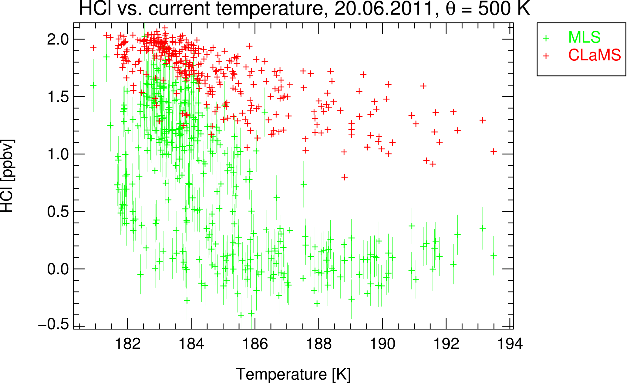
Figure 7MLS observations of HCl mixing ratio on 20 June 2011 in the vortex core (Φ_e>75^∘ S) on the 500 K potential temperature level. The individual data points are plotted as a function of temperature given by ERA-Interim (green symbols). The error bars show the given measurement precision. The corresponding CLaMS results are given as red symbols.

Download

To find out more about the characteristics of the potentially missing process that could explain the difference between simulated and observed HCl, we focus on the comparison between simulations and observations for the vortex-core data points on the 500 K level for 20 June (data from about 300 MLS profiles). This is a time and location when, in both the model and the observations, the HCl depletion after the initial titration step is ongoing. From that, we can get hints about the possible missing process (or processes).

First, we investigate whether the missing process is correlated with temperature. This would be the case if the depletion of HCl is caused by uptake on PSC particles, for example, into the available liquid PSC particles as suggested by the empirical correction in Wohltmann et al. (2017). Similar to HNO₃, HCl is soluble in liquid aerosols. The solubility of HCl in the liquid aerosols given by the parameterisation of Carslaw et al. (1995) is included in the CLaMS chemistry module. Although the simulations do not show any significant HCl uptake, it may be that underlying parameters like Henry's law constant are not accurately represented in the parameterisation as suggested by Wohltmann et al. (2017). The uptake of HCl into the liquid aerosol particles should be strongly temperature dependent (Carslaw et al., 1994), with the largest expected effect for the lowest temperatures. To examine such a hypothesis, the chosen subset of MLS data points and corresponding CLaMS points are plotted as function of temperature in Fig. 7. The temperature for all data points in this subset is below 194 K, suggesting that PSCs should exist at the observation locations shown, which is supported by the MIPAS PSC database (Spang et al., 2018). The simulations and observations in Fig. 6 suggest that the first titration step is completed by 20 June. The temperature dependence of the difference between observations and the simulation does not, however, suggest a missing uptake of HCl into the particles. The largest discrepancies between simulations and observations are found for higher temperatures. Therefore, the uptake of a significant fraction of HCl into the PSC particles seems to be an unlikely explanation for the discrepancy shown between Figs. 2 and 3. However, it cannot be excluded that this dependency is caused by a combination of more than one unknown process.

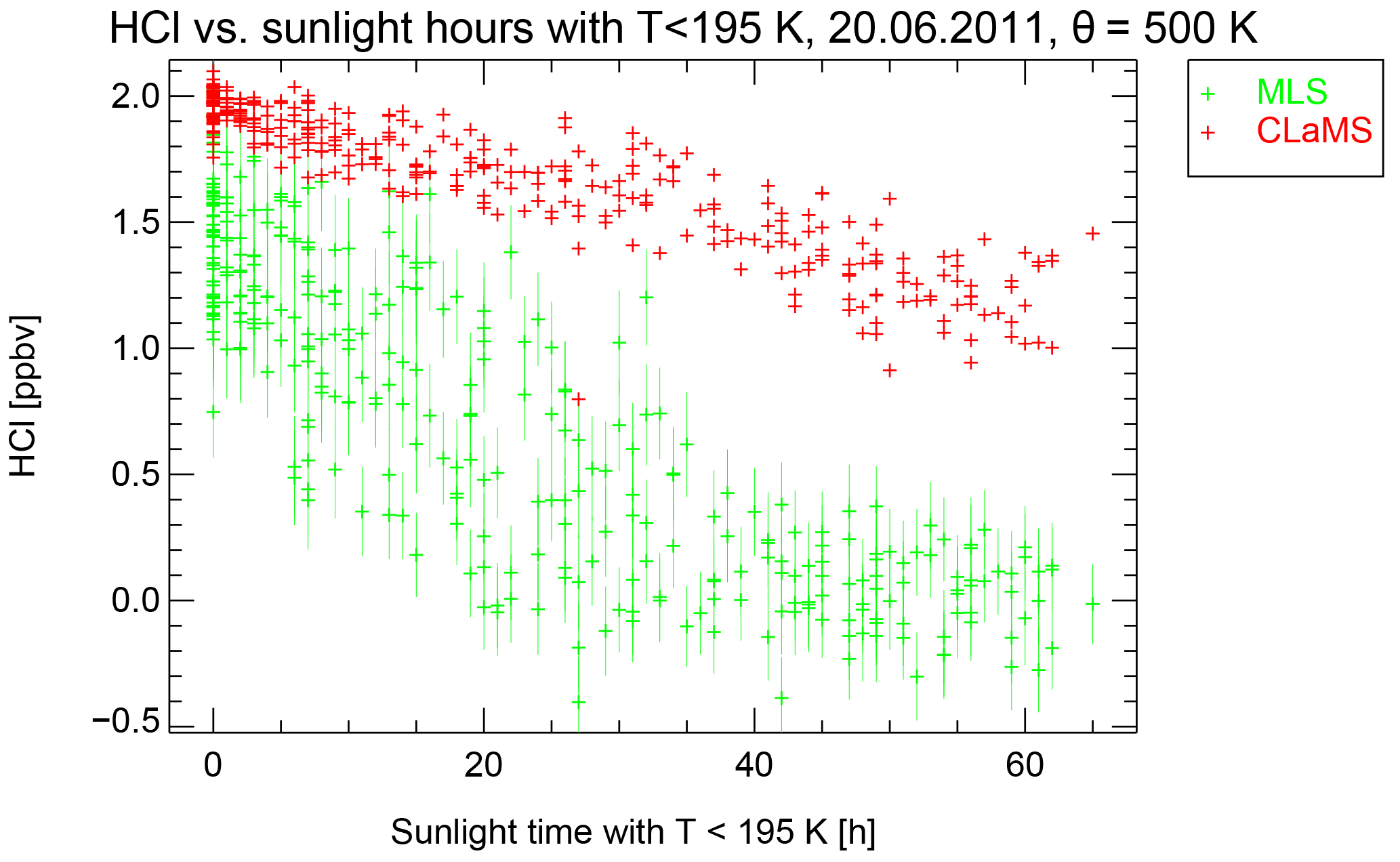
Figure 8MLS observations of HCl mixing ratio that are also displayed in Fig. 7 plotted against sunlight time with temperatures below 195 K derived from the backward trajectories (green symbols) and the corresponding CLaMS results (red symbols).

Download

Although the HCl depletion is not directly correlated with temperature, it seems likely that the missing process should require temperatures low enough for heterogeneous chlorine activation on PSCs or cold aerosols. We examine whether the missing process requires sunlight by investigating the history of the same observed air masses using 30-day back trajectories calculated by the CLaMS trajectory module. From the trajectories, we determined how long the air mass experienced sunlight and also how long they were exposed to temperatures below 195 K, a typical value below which PSCs can form and heterogeneous chemistry becomes important. Here, we used solar zenith angles below 95^∘ for the definition of sunlight time (Rex et al., 2003).

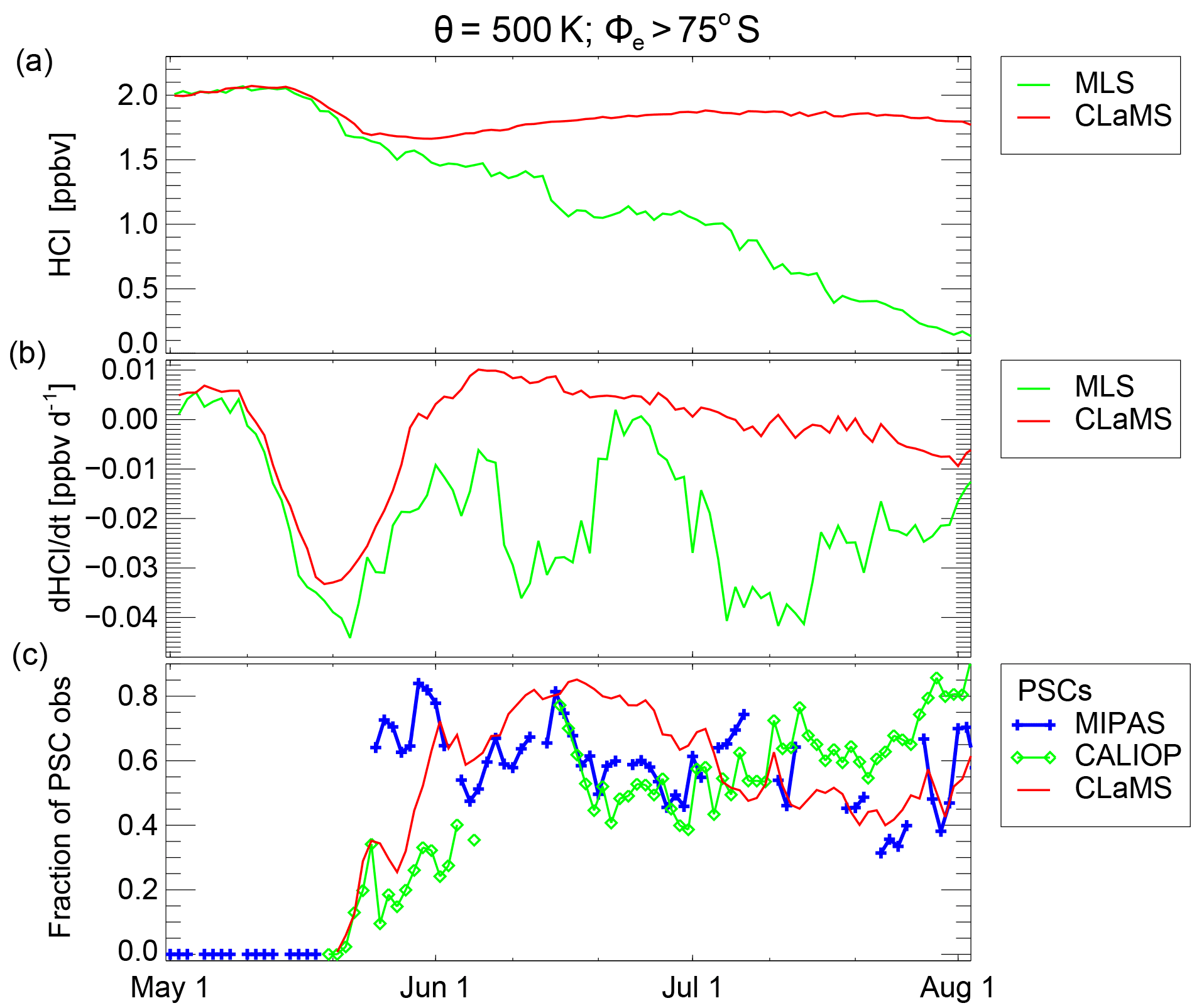
Figure 9Vortex-core averages (Φ_e>75^∘ S, θ=500 K) of HCl, its time derivative and PSC occurrence frequency. Panel (a) shows HCl mixing ratios from CLaMS and MLS. Panel (b) shows the corresponding time derivative dHCl∕dt (smoothed as a 6-day running mean). Panel (c) shows the fraction of MIPAS and CALIOP observations with Φ_e>75^∘ S on the 500 K potential temperature level that are classified as PSCs. It also shows the corresponding CLaMS results. The symbols are connected with coloured lines except for days without PSC information.

Download

Figure 8 shows the individual observed HCl mixing ratios as a function of the time spent in sunlight and below 195 K as green symbols. Red symbols show the corresponding simulated HCl mixing ratios. There seems to be a clear anticorrelation between the time spent in sunlight below 195 K and HCl mixing ratios. This suggests that the missing process may both require sunlight and low temperatures in the presence of PSCs.

To further clarify the temporal development of the HCl discrepancy, Fig. 9 shows also the rate of HCl change dHCl∕dt calculated from the time series of HCl within the grid box in the equivalent latitude/potential temperature space for each day (Fig. 9b). It is evident that the first titration step caused by the heterogeneous reaction of HCl with ClONO₂ is reproduced correctly in the simulation. After that step, HCl decreases particularly strongly during two periods in mid-June and mid-July. These periods are correlated with a high occurrence fraction of PSCs as shown in Fig. 9c. Both the HCl depletion rate and PSC occurrence seem to have relative maxima around 11 June (i.e. large rate of HCl depletion), minima around 23 June and again maxima between 5 and 12 July. The PSC occurrence fraction is shown for both MIPAS and CALIOP observations, which are broadly consistent for the overlapping observation times. The corresponding CLaMS PSC occurrence fractions are also shown. The only significant difference between MIPAS and CALIOP is in late May where MIPAS detects a large fraction of potentially small STS particles that could not be detected by CALIOP. Also in the beginning, these STS detections are pole-centred and therefore partly missed by the limited latitudinal coverage of the CALIPSO satellite. The anticorrelation between dHCl∕dt and the PSC occurrence fraction is a further indication that PSCs may be relevant here. Possible processes missing in the formulation of the model that could explain the HCl discrepancy are investigated in the following section.

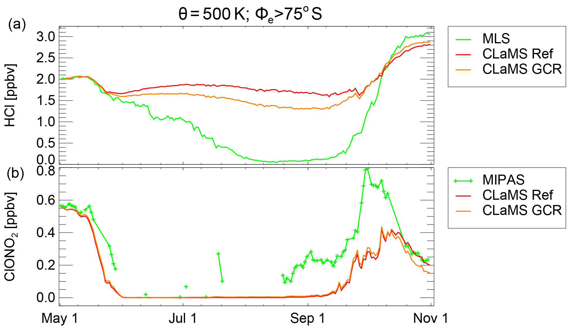
Figure 10Average mixing ratios in the vortex core (Φ_e>75^∘ S, θ=500 K) of HCl (a) and ClONO₂ (b). Green lines show MLS and MIPAS observations, respectively. CLaMS results are shown for the reference simulation (red) and the simulation with incorporated ionisation from galactic cosmic rays (GCRs, orange).

Download

The required missing process (or processes) should clearly improve the characteristic difference between observed and simulated HCl mixing ratios (Figs. 2 and 3). By incorporating different processes into a model, we can investigate the “fingerprint” of the corresponding change to the model results. This method will not provide a proof of whether a hypothetical process occurs in reality. However, it can help to exclude hypothetical processes when they cause different “fingerprints” that can be contrasted with observations. In the following subsections, different hypotheses for the missing processes are investigated by incorporation into the model CLaMS.

6.1 Ionisation from galactic cosmic rays

One well-known process that is often neglected in simulations of stratospheric chemistry is the ionisation of air molecules by galactic cosmic rays. Galactic cosmic rays (GCRs) provide an additional source of NO_x and HO_x (Warneck, 1972; Rusch et al., 1981; Solomon et al., 1981; Müller and Crutzen, 1993). The additional source of OH and NO in the polar stratosphere can trigger an HCl sink through the following reaction chains:

$$\begin{array}{ll}{\displaystyle }& {\displaystyle }\mathrm{NO}+{\mathrm{O}}_{\mathrm{3}}\to {\mathrm{NO}}_{\mathrm{2}}+{\mathrm{O}}_{\mathrm{2}}\\ {\displaystyle }& {\displaystyle }{\mathrm{NO}}_{\mathrm{2}}+\mathrm{ClO}\stackrel{\mathrm{M}}{\mathit{⟶}}{\mathrm{ClONO}}_{\mathrm{2}}\\ {\displaystyle }& {\displaystyle }\mathrm{HCl}+{\mathrm{ClONO}}_{\mathrm{2}}\stackrel{\mathrm{het}}{\mathit{⟶}}{\mathrm{Cl}}_{\mathrm{2}}+{\mathrm{HNO}}_{\mathrm{3}}\end{array}$$

and

$$\begin{array}{ll}{\displaystyle }& {\displaystyle }\mathrm{OH}+{\mathrm{O}}_{\mathrm{3}}\to {\mathrm{HO}}_{\mathrm{2}}+{\mathrm{O}}_{\mathrm{2}}\\ {\displaystyle }& {\displaystyle }{\mathrm{HO}}_{\mathrm{2}}+\mathrm{ClO}\stackrel{\mathrm{M}}{\mathit{⟶}}\mathrm{HOCl}+{\mathrm{O}}_{\mathrm{2}}\\ {\displaystyle }& {\displaystyle }\mathrm{HOCl}+\mathrm{HCl}\stackrel{\mathrm{het}}{\mathit{⟶}}{\mathrm{Cl}}_{\mathrm{2}}+{\mathrm{H}}_{\mathrm{2}}\mathrm{O}.\end{array}$$

These reaction chains are only effective in the presence of heterogeneously active particle surfaces (cold binary aerosols or PSCs) and in the presence of sunlight since the ClO molecule would be converted into Cl₂ O₂ in darkness. To investigate this effect, the NO_x and HO_x sources from cosmic-ray-induced ionisation pairs were incorporated into the chemistry module of CLaMS. The ionisation rate was induced after Heaps (1978) using the efficiency eff_NO=1.25 and eff${}_{{\mathrm{HO}}_x}=\mathrm{2}$ for the formation of NO and OH per ionisation, respectively (Jackman et al., 2016). Fig. 10 shows the corresponding vortex-core average (${\mathrm{\Phi }}_e>\mathrm{75}{}^{\circ }$ S) on the 500 K level for the reference simulation and the simulation including induced ionisation by the GCRs. Indeed, including such an ionisation rate in the model does introduce an accelerated HCl decomposition in the polar vortex where active chlorine exists. However, the effect is too small to explain the CLaMS HCl discrepancy shown in Sect. 4. By early August, the HCl discrepancy shown here is reduced by about 20 %. Even though there are newer estimates of the GCR-induced ionisation rate (Usoskin et al., 2010; Jackman et al., 2016), they are not significantly larger, so a severe underestimation of the ionisation rate seems unlikely.

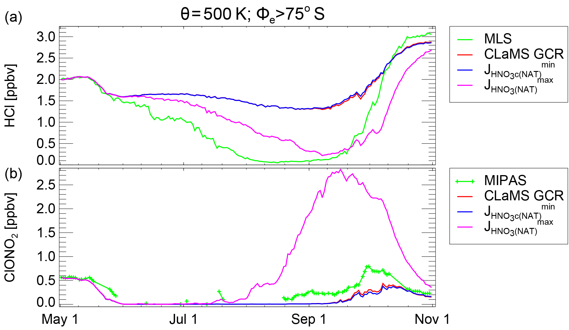
Figure 11Average mixing ratios in the vortex core (Φ_e>75^∘ S, θ=500 K) of HCl (a) and ClONO₂ (b). Green lines show MLS and MIPAS observations, respectively. The red line shows the CLaMS simulation including GCR-induced ionisation. The blue and pink lines correspond to simulations with additional photolysis of particulate HNO₃ using the lower and upper estimates, respectively, as described in the text.

Download

6.2 Photolysis of particulate HNO₃

Besides the photolysis of gas-phase HNO₃, it may be possible that the HNO₃ bound in PSC particles also photolyses directly. Evidence for this comes from studies which have shown that nitrate photolysis from snow surfaces is a significant source of NO_x at the Earth's surface (e.g. Honrath et al., 1999; Dominé and Shepson, 2002) and that nitrate photolysis in the quasi-liquid layer in laboratory surface studies is enhanced in the presence of halide ions due to a reduced solvent cage effect (Wingen et al., 2008; Richards et al., 2011). These studies suggest that photolysis of dissolved HNO₃ in PSC particles, including STS droplets, may be possible. If such a process could liberate NO_x or HO_x into the gas phase from the particle phase, it could also cause HCl depletion by the reaction chains mentioned above. However, we note that such a process is not yet proven. Wegner (2013) investigated this hypothesis by implementing this process into the model SD-WACCM. He used the cross section for the NO₃⁻ ion (Chu and Anastasio, 2003), with a quantum yield of 0.3 reflecting relatively high values seen on some surfaces in laboratory experiments (Abida et al., 2012). These simulations indicated that due to the low solar elevation in austral winters, the onset of HCl depletion in June cannot be reproduced by adding this process. Furthermore, this NO_x source would cause an overestimation of ClONO₂ at higher solar elevation in September.

Here, we extend the investigation by Wegner (2013) by including possible upper and lower limits for this process, as the photolysis of particulate HNO₃ on PSCs has not been investigated in detail. Laboratory measurements show that combined absorption cross sections of HNO₃(aq) and NO₃ in bulk solutions are significantly larger than those in the gas phase (Chu and Anastasio, 2003; Svoboda et al., 2013). Quantum yields in the aqueous bulk phase are small, ≈1 % or less (Warneck and Wurzinger, 1988; Benedict et al., 2017), increasing to a few percent in the quasi-liquid layers (McFall et al., 2018). However, quantum yields on other surfaces may be much larger (Abida et al., 2012), and such large values are also suggested by strong NO_x emissions from nitrate-containing particles exposed to UV radiation (Reed et al., 2017; Ye et al., 2016; Baergen and Donaldson, 2013). As a lower limit for the photolysis of particulate HNO₃, we apply also the gas-phase photolysis of HNO₃ to the NAT particles with a quantum yield of 1. As an estimate for the upper limit, we use observations of the absorption cross sections in ice by Chu and Anastasio (2003) and also a quantum yield of 1. The absorption cross sections employed and the photolysis rates derived from those are shown in Fig. S5 of the Supplement. As in Fig. 10, Fig. 11 shows the HCl and ClONO₂ data, the CLaMS GCR simulation (blue) and the upper and lower limits as described above. The lower limit (blue lines) is not very different from the CLaMS simulation without this process. In the simulation for the upper limit, an additional faster depletion of HCl is clearly visible. However, throughout the month of June, the effect is not large enough to fully explain the remaining HCl discrepancy. Furthermore, the simulation indicates that this process would significantly enhance the chlorine deactivation into ClONO₂ in late August and September. Therefore, the upper limit simulation appears not to be the process that would resolve the HCl discrepancy. Potentially, this process with a lower quantum yield may explain the small discrepancy in ClONO₂ in September. The fingerprint of a photolysis-like process increases with solar elevation and therefore would be much stronger in September than in June. However, there may be a similar process independent of the solar zenith angle that could decompose condensed-phase HNO₃ as discussed in the following subsection.

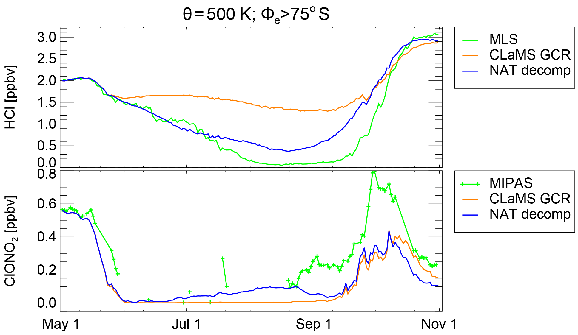
Figure 12As Fig. 10 but for CLaMS simulation with hypothetical NAT decomposition. CLaMS results are shown for the GCR simulation (orange) and the NAT decomp simulation (blue).

Download

Figure 13CLaMS simulation results for HCl of the sensitivity NAT decomp simulation averaged in equivalent latitude/potential temperature space displayed as in Figs. 2 and 3.

Download

6.3 Decomposition of particulate HNO₃

A similar hypothesis to that described above would be the decomposition of the condensed-phase HNO₃ by a process other than photolysis. A more steady decomposition throughout the polar winter could be triggered, for example, by GCRs instead of by photolysis. For this hypothesis, sunlight or at least twilight would still be required to form sufficient ClO from the decomposition of the nighttime reservoir Cl₂O₂. Over the poles especially, secondary electrons from GCRs that do not have enough energy to decompose air molecules may still be able to interact with HNO₃ on the PSCs. In Fig. 12, the HCl discrepancy in June and July steadily increases with time in the presence of NAT or ice PSCs. To achieve the observed HCl depletion rate on the 500 K potential temperature level, about 1 % of the condensed HNO₃ per day needs to be liberated into the gas phase. The exact mechanism by which this could occur needs to be clarified, but to investigate the impact of this hypothesis we performed a test simulation in which the HNO₃ on NAT is decomposed into NO₂ + OH at a constant rate of 10⁻⁷ s⁻¹, independent of altitude (labelled “NAT decomp”).

Figure 14Simulated vortex mean ozone profile for 1 October 2011 from MLS (green) and different model runs of SD-WACCM (blue), TOMCAT/SLIMCAT (pink) and CLAMS (GCR, orange). The results from the “NAT decomp” sensitivity simulation are shown as a red dashed line. The grey line corresponds to the CLaMS passive ozone tracer and the difference with the other lines indicates the chemical ozone depletion.

Download

Figure 12 shows the simulated HCl mixing ratios in Φ_e ∕ θ space. Even though not every detail of the observations is reproduced, it is evident that this simulation reproduces the observations much better than any of the hypotheses discussed above. The rate of the hypothetical process was chosen such that the HCl depletion on the 500 K level is well represented. It is evident that above this level this rate should increase. However, it does not seem appropriate to speculate further here.

One further piece of evidence for the hypothesis that a possible NO_x source from PSC decomposition exists is given by the comparison with ClONO₂ data. Figure 12 shows the time development of vortex-core mixing ratios of HCl and ClONO₂ on the 500 K potential temperature level. The blue line in the top panel demonstrates that on this level the observed HCl depletion is represented by the NAT decomp simulation. The MIPAS observations of ClONO₂ are intermittent since many observations are blocked by the presence of PSCs. However, the remaining observations indicate low mixing ratios in the range between 0.05 and 0.1 ppbv between late May and late August. These observations are better reproduced by the NAT decomp simulation than both other simulations in which ClONO₂ is nearly zero between early June and the end of September. From late August to October, simulations of ClONO₂ are lower than the simulation. The only sensitivity run that exceeds the observations of ClONO₂ is that with the upper limit for photolysis of particulate HNO₃ which also demonstrates that an additional NO_x source would increase the ClONO₂ mixing ratio.

The change in chlorine activation by this hypothetical process may also be visible in a comparison with MLS ClO, for which the model output has to be calculated exactly for the location and local time of the observations. For the area of interest defined above (20 June, θ=500 K), the observations in the vortex core are, however, at solar zenith angles such that the ClO mixing ratios are mostly zero within experimental uncertainty. For measurements near the vortex edge, no significant ClO differences are induced by this hypothetical process (compare Figs. S6 and S7 of the Supplement).

The complete fingerprint of the 3-D HCl development similar to Figs. 2 and 3 is shown in Fig. 13. Although differences remain, this sensitivity experiment simulates the HCl observations much better than any other CLaMS simulation discussed here.

We now investigate the impact of HCl processing on ozone, since the amount of active chlorine in the polar stratosphere is essential for the determination of chemical ozone loss. All three participating models do simulate the chemical ozone loss and the formation of the ozone hole sufficiently well. Figure 14 shows the simulated vortex-average ozone profile on 1 October for the different models in combination with the passive ozone tracer from CLaMS. The difference between the two profiles corresponds to the chemical ozone loss over the winter until this time. The potential process that was included in the NAT decomp simulation increases chlorine activation significantly, especially in the polar winter. This might also affect the simulated ozone depletion. However, the difference in chlorine activation is especially large in the rather dark vortex core, where chemical ozone depletion rates are small.

The impact of the hypothetical NAT decomposition processes on polar ozone depletion would cause an additional 0.2 ppmv vortex-average ozone depletion on the 500 K level as shown in Fig. 14. Figure 15 shows the simulated chemical ozone depletion for the three CLaMS simulations, the reference simulation, the simulation including GCR-induced ionisation and the simulation also including the hypothetical NAT decomposition. The ozone depletion is also shown for the simulation for the Arctic winter 2015/2016 employing the same model setup. Although it is clear that an increase in chlorine activation yields more ozone depletion, the overall effect on ozone depletion of this additional hypothetical process is rather low. The increase of column ozone loss in the vortex core due to GCR-induced ionisation ranges from 2 to 3 %. The additional column ozone loss due to the hypothetical NAT decomposition is calculated to be about 1.8 % in the Antarctic winter and only 0.6 % in the Arctic winter.

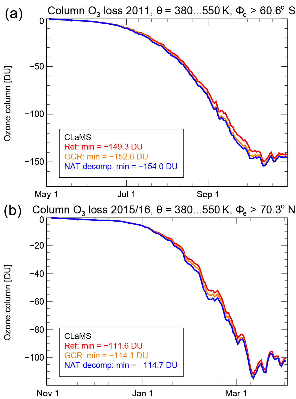
Figure 15Simulated column ozone loss between 380 and 550 K potential temperature for the Antarctic winter 2011 (a) and the Arctic winter 2015/2016 (b). The results are shown for different sensitivity simulations. Red lines correspond to the reference simulation, orange lines to the simulation including GCR-induced ionisation, and blue lines to the NAT decomp simulation. The legend also indicates the maximum column ozone loss amount of each simulation.

Download

MLS data were obtained from ftp://acdisk.gsfc.nasa.gov//data/s4pa/Aura_MLS_Level2/, last access: 20 November 2017. MIPAS data are taken from http://share.lsdf.kit.edu/imk/asf/sat/mipas-export, last access: 8 June 2018. The model data averages on potential temperature surfaces from CLaMS, SD-WACCM, and TOMCAT/SLIMCAT that were used for creating Figs. 2–4, 6, and 9–15 are available from https://datapub.fz-juelich.de/slcs/clams/hcl_discrepancy/. The CCMI model simulations from SD-WACCM can be requested at https://www.earthsystemgrid.org/search.html?Project=CCMI1. For more detailed model data, please contact the model authors.

The supplement related to this article is available online at: https://doi.org/10.5194/acp-18-8647-2018-supplement.

The authors declare that they have no conflict of interest.

This article is part of the special issues “The Polar Stratosphere in a Changing Climate (POLSTRACC) (ACP/AMT inter-journal SI)” and “Quadrennial Ozone Symposium 2016 – Status and trends of atmospheric ozone (ACP/AMT inter-journal SI)”. It is not associated with a conference.