the Creative Commons Attribution 4.0 License.
the Creative Commons Attribution 4.0 License.
 | 15 Jun 2018
Maximizing ozone signals among chemical, meteorological, and climatological variability
Benjamin Brown-Steiner
Noelle E. Selin
Ronald G. Prinn
Erwan Monier
Simone Tilmes
Louisa Emmons
Fernando Garcia-Menendez
The detection of meteorological, chemical, or other signals in modeled or observed air quality data – such as an estimate of a temporal trend in surface ozone data, or an estimate of the mean ozone of a particular region during a particular season – is a critical component of modern atmospheric chemistry. However, the magnitude of a surface air quality signal is generally small compared to the magnitude of the underlying chemical, meteorological, and climatological variabilities (and their interactions) that exist both in space and in time, and which include variability in emissions and surface processes. This can present difficulties for both policymakers and researchers as they attempt to identify the influence or signal of climate trends (e.g., any pauses in warming trends), the impact of enacted emission reductions policies (e.g., United States NOx State Implementation Plans), or an estimate of the mean state of highly variable data (e.g., summertime ozone over the northeastern United States). Here we examine the scale dependence of the variability of simulated and observed surface ozone data within the United States and the likelihood that a particular choice of temporal or spatial averaging scales produce a misleading estimate of a particular ozone signal. Our main objective is to develop strategies that reduce the likelihood of overconfidence in simulated ozone estimates. We find that while increasing the extent of both temporal and spatial averaging can enhance signal detection capabilities by reducing the noise from variability, a strategic combination of particular temporal and spatial averaging scales can maximize signal detection capabilities over much of the continental US. For signals that are large compared to the meteorological variability (e.g., strong emissions reductions), shorter averaging periods and smaller spatial averaging regions may be sufficient, but for many signals that are smaller than or comparable in magnitude to the underlying meteorological variability, we recommend temporal averaging of 10–15 years combined with some level of spatial averaging (up to several hundred kilometers). If this level of averaging is not practical (e.g., the signal being examined is at a local scale), we recommend some exploration of the spatial and temporal variability to provide context and confidence in the robustness of the result. These results are consistent between simulated and observed data, as well as within a single model with different sets of parameters. The strategies selected in this study are not limited to surface ozone data and could potentially maximize signal detection capabilities within a broad array of climate and chemical observations or model output.
- Article
(3799 KB) -
Supplement
(1713 KB) - BibTeX
- EndNote


The capability to detect air quality signals – be they meteorological, chemical, or of some other type – is a fundamental component of modern climate science and atmospheric chemistry. The debate over the existence or length of a global warming hiatus (Lewandowsky et al., 2015; Roberts et al., 2015; Medhaug et al., 2017) and research examining the time of emergence of climatological (Weatherhead et al., 2002; Deser et al., 2012; Hawkins and Sutton, 2012; de Elía et al., 2013; Schurer et al., 2013), meteorological (Giorgi and Bi, 2009; King et al., 2015), chemical (Camalier et al., 2007; Strode and Pawson, 2013; Barnes et al., 2016; Garcia-Menendez et al., 2017), and other sectoral signals (e.g., Monier et al., 2016) embody an accumulation of techniques and strategies for filtering noise (due to natural variability) and maximizing the capability to detect statistically significant signals and trends in noisy data. It is well established that temporal averaging (e.g., Lewandowsky et al., 2015) and spatial averaging (e.g., Frost et al., 2006; Hawkins and Sutton, 2012; Barnes et al., 2016) can enhance signal detection capabilities in atmospheric data. Here we extend this research by quantifying the impact of both spatial and temporal averaging – individually and in combination – of surface ozone on the magnitude of the calculated variability, which is largely driven by the influence of meteorological variability on atmospheric chemistry (e.g., Jacob and Winner, 2009). We offer recommendations for strategically averaging in space and time to maximize signal detection capabilities. In particular, we examine estimates of mean ozone and of the ozone variability that results from meteorology, although our approach can be generalized to other air quality applications.
For observed ozone data, strategies for reducing spatial and temporal noise are limited: a longer time series is needed, more observations need to be made, or the spatial region over which the ozone observations are being averaged needs to be enlarged. For surface ozone estimates using models, however, there exist a variety of strategies for reducing the noise (due to chemical and meteorological variability) relative to the strength of the signal, although they cluster into three main types. The first strategy is to average or combine multiple runs of structurally different models under the assumption that errors, biases, and uncertainties within the individual models are reduced and the multi-model or multi-dataset mean is a best estimate of the actual, aggregated ozone field. This is most notably done with multi-model ensembles within the Atmospheric Chemistry and Climate Model Intercomparison Project (ACCMIP) framework (Lamarque et al., 2013; Young et al., 2013; Stevenson et al., 2013), and this approach tends to assume that all members in the ensemble are independent and equally skillful. This assumption, however, may result in a loss of some valuable information (Knutti, 2010). Another form of this strategy is to run multiple model runs within a single model, but under different initial conditions or sets of parametric assumptions (e.g., Deser et al., 2012; Monier et al., 2013, 2015; Kay et al., 2015; Garcia-Menendez et al., 2015, 2017). This approach cannot address structural uncertainties and internal (unforced) variability between models, but is capable of identifying parametric uncertainties within a single model.
The second strategy to reduce ozone variability is to expand the temporal averaging window, which can influence the interpretation of the determined ozone value (e.g., Brown-Steiner et al., 2015). The Environmental Protection Agency (EPA) National Ambient Air Quality Standard (NAAQS) for ozone (US EPA, 2015) explicitly takes this into account, both in the length of the averaging period (daily maximum 8 h average) and the selection criteria for the standard (fourth highest over the previous 3 years). The calculated ozone variability can be further reduced by utilizing even longer averaging periods, such as monthly (e.g., Rasmussen et al., 2012), seasonal (e.g., Fiore et al., 2014; Barnes et al., 2016), annual, or decadal mean values (e.g., Garcia-Menendez et al., 2017). This strategy is analogous to the averaging of meteorological data to derive a climate signal, and, just as Lewandowsky et al. (2015) recommend averaging 17 or more years in order to achieve climatological estimates of temperature trends, there is a growing body of literature recommending averaging short-timescale chemical variability (what could be called chemical weather, see Lawrence et al., 2005) for 15 or more years (e.g., Garcia-Menendez et al., 2017) in order to achieve an estimate of what could be called the chemical climate (see Möller, 2010).
The third strategy to reduce ozone variability is to average surface ozone values over larger spatial regions, and, while there is a significant body of literature discussing the capability and interpretation of coarse-resolution model representations of the sub-grid-scale heterogeneity (Pyle and Zavody, 1990; Searle et al., 1998; Wild and Prather, 2006), there are few that strategically expand the spatial scale over which averaging is applied in order to maximize signal detection capabilities. This strategy has been applied in other fields of the atmospheric sciences as well as for general gridded datasets (e.g., Pogson and Smith, 2015), and spatial averaging has been suggested as a means of reducing temperature variability and smoothing biases at the smallest spatial scales within a single model run (Räisänen and Ylhäsi, 2011). This “scale problem” has also been noted as an important consideration when analyzing aerosol indirect effects (McComiskey and Feingold, 2012) and for the detection and attribution of extreme weather events (Angélil et al., 2017).
Our objective in this study is to provide a framework for selecting spatial and temporal averaging scales that reduces the uncertainty in analyzing ozone signals and limits the likelihood of overconfidence in an estimate of surface ozone that arises from meteorological variability. This type of framework can be useful from two different research perspectives. The first research perspective has a priori an ozone estimate (either observed or modeled) at a certain spatial and temporal scale (e.g., a 3-year simulation of surface ozone over the northeastern US) and aims to quantify the likelihood that this estimate is representative of the long-term ozone behavior (rather than overly sensitive to meteorological variability of that particular 3-year period). Since ozone is strongly influenced by natural fluctuations in meteorology (Jacob and Winner, 2009; Jhun et al., 2015) and since extremes in surface ozone and temperature tend to co-occur (Schnell and Prather, 2017), atypically hot or cold periods can strongly influence ozone behavior over short timescales.
The second research perspective is to identify an ozone signal of a certain magnitude (or threshold) and decide what spatial and temporal averaging scales are needed to best identify that signal. The ozone signal could be large (e.g., determining the effectiveness or compliance with a 5 ppbv incremental reduction of the EPA NAAQS for ozone; US EPA, 2015) or small (e.g., identifying annual ozone trends within the US, which Cooper et al., 2012, show can be on the order of 0.10–0.45 ppbv) and can be highly sensitive to spatial and temporal heterogeneity and meteorological variability. Barnes et al. (2016) found that surface ozone trends over 20-year periods can vary by ±2 ppbv due solely to climate variability, while interannual variability can be on the order of ±15 ppbv (Fiore et al., 2003; Tilmes et al., 2012; Lin et al., 2014) and day-to-day variability can be even larger, extending regularly from near-background levels of 40–50 ppbv up to 100 ppbv during the summertime (Fiore et al., 2014).
In this study, we quantify the impact of both temporal and spatial averaging on the calculated ozone variability – due solely to meteorological variability – in order to maximize the capability to detect signals. We use simulated ozone (with the Community Atmosphere Model with Chemistry, CAM-chem) and observational data (with the EPA's Clean Air Status and Trends Network, CASTNET) within the United States in order to answer the following four questions. (1) Within a given dataset (model or observations), with both spatial and temporal coverage, what is the magnitude of the ozone variability due to meteorology at the smallest scale, and how does spatial and temporal averaging reduce this variability? (2) Are there combinations of temporal and spatial averaging scales that maximize the signal detection capability for surface ozone data? (3) How sensitive are the above strategies to different configurations (i.e., emissions, meteorology, and climate) of the CAM-chem modeling framework? And (4) how could they be applied to other datasets (chemical, meteorological, or climatological)? We limit our focus to spatial scales within the United States as it has high spatial and temporal variability and numerous observations, and since averaging over larger regions (e.g., the Northern Hemisphere, or the globe) would produce a smaller calculated variability.
In Sect. 2, we describe the CAM-chem model and our simulations, as well as the CASTNET observational database and the regional definitions used throughout this paper. In Sect. 3 we quantify the temporal and spatial variability of surface ozone, show how temporal and spatial averaging reduces the calculated ozone variability, and demonstrate the spatial heterogeneity of the calculated ozone variability. In Sect. 4, we discuss the potential strategies that could be used to maximize ozone signal detection due to meteorological variability, explore uncertainties, and make recommendations for future research.
We examine both present-day (one simulation and one observed dataset) and future (two simulations) surface ozone in this study. For present-day analysis, we simulate surface ozone using CAM-chem, a component of the Community Earth System Model (CESM) and available observations within the US from the EPA CASTNET database. For future analysis, and in order to examine the potential for patterns of variability to change in the future, we utilize two existing simulations of CAM-chem conducted by Garcia-Menendez et al. (2017). Much of this analysis is conducted using the R language (R Project, https://www.r-project.org/, last access: 7 June 2018). Here we summarize each of the three datasets and our approach to our analysis in Sect. 3.
2.1 CAM-chem
The present-day simulation (MOZ_2000) was conducted using CAM-chem model version 1.2.2, with the CAM4 atmospheric component (see Tilmes et al., 2015, 2016, for model description and evaluation). The model has been used extensively for a wide range of atmospheric chemistry research and is included in the ACCMIP (Lamarque et al., 2012; Young et al., 2013, and references therein). We conduct our simulations using the Model for Ozone and Related chemical Tracers version 4 (MOZART-4) chemical mechanism (Emmons et al., 2010), which is a full tropospheric chemical mechanism integrated into CAM-Chem (e.g., Lamarque et al., 2012; Tilmes et al., 2015). Offline forced meteorology is taken from the Modern-Era Retrospective analysis for Research and Applications (MERRA) reanalysis product (Rienecker et al., 2011) for 26 meteorological years (1990–2015). Additional model evaluation and comparisons to surface and ozonesonde observations can be found in Brown-Steiner et al. (2018). This simulation has 56 vertical levels – adopted from MERRA meteorology – as well as 96 latitudinal and 144 longitudinal grid cells. We aim to isolate the variability to the meteorologically driven impact on atmospheric chemistry so we repeat year-2000 anthropogenic emissions from the ACCMIP inventory (Lamarque et al., 2012) as well as all non-biogenic emissions for all meteorological years and include specified long-lived stratospheric species (O3, NOx, HNO3, N2O, N2O5) as in MOZART-4 (Emmons et al., 2010), an online biogenic emissions model MEGAN (Guenther et al., 2012), and forced sea ice and sea surface temperatures to year-2000 historical conditions. Like many state-of-the-art chemical tracer models, the CAM-chem exhibits some biases, most notably for our purposes a high bias in simulated surface ozone in the eastern US (e.g., Lamarque et al., 2012; Brown-Steiner et al., 2015; Travis et al., 2016; Barnes et al., 2016). Recent efforts have been successful in partially reducing these biases (e.g., Sun et al., 2017).
We also include two reference simulations of the future climate, MOZ_2050 and MOZ_2100 (simulating the meteorological years 2035–2065 and 2085–2115, respectively), using the CESM CAM-chem simulations described in detail by Garcia-Menendez et al. (2017) with one set of initial condition data and a climate sensitivity of 3.0 ∘C. These simulations do not include projections of any changes in future emissions. Compared to the present-day simulation (MOZ_2000), these future simulations (MOZ_2050 and MOZ_2100) have several parametric differences: the model version is 1.1.2 (see Tilmes et al., 2015, and references for information on model development), the atmospheric component is CAM3, the emissions (which are held constant at year-2000 levels) are from the Precursors of Ozone and their Effects in the Troposphere database (see Garcia-Menendez et al., 2017), and the meteorology is derived from a linkage between the Massachusetts Institute of Technology Integrated Global System Model (MIT IGSM) and the CESM CAM model (Monier et al., 2013), and as such has 26 vertical levels. For a full description of these simulations, see Garcia-Menendez et al. (2017).
2.2 CASTNET
The observational database comes from the EPA Clean Air Status and Trends Network (CASTNET), which has more than 90 surface observational sites within the United States and has been collecting hourly surface meteorological and chemical data since 1990 (US EPA, 2016 and https://www.epa.gov/castnet, last access: 7 June 2018). We collected data from all sites that reported complete ozone data from each year and removed data that was marked invalid within the downloaded EPA files. The number of sites that matched these criteria varied from year to year, but generally we have between 55 and 94 sites throughout the 1991–2014 period. The CASTNET observational network is located primarily in rural sites and thus is considered to be a reasonable comparison to coarse grid-cell model output (e.g., Brown-Steiner et al., 2015; Phalitnonkiat et al., 2016). Since a notable trend in observed ozone data exists, especially in the northeastern US (Frost et al., 2006), and since the simulations have no change in anthropogenic emissions, and thus no ozone trend, we detrended the CASTNET data for each of the four averaging regions (described below) using a simple linear regression.
2.3 Telescoping regional definitions
In order to isolate the impact of the size of the spatial scale over which ozone data are averaged, we analyze ozone data at different spatial scales. The largest region considered is the entire continental US, while the smallest regions considered are at the individual grid-cell level of the CESM CAM-chem model (1.9 × 2.5∘ latitude and longitude). Data and statistics for the other regions (i.e., the midwestern and southeastern US) are included in the Supplement but do not alter the conclusions we draw from the northeastern US. For CESM CAM-chem data, we averaged all grid cells within each region, while for the CASTNET data we first average sites within each corresponding CESM CAM-chem grid cell and then average these data together. These telescoping regions are shown in Fig. 1.

Figure 1Telescoping spatial regions included in this study. The largest scale we consider is the continental US (outer border). We focus on the eastern US by subdividing into three subregions: the midwest (blue), northeast (black), and southeast (red). Within each subregion we telescope into a 3 × 3 grid cell (yellow) a 2 × 2 grid cell (purple), and a 1 × 1 grid cell (green). In the paper, we only show a subset of these telescoping regions, and we include the rest in the Supplement.
2.4 Temporal averaging windows
To explore the impact of temporal averaging, we examine ozone across a range of temporal averaging windows, from 1 day up to the full 26 years for the CESM data (1990–2015), the full 24 years for the detrended CASTNET data (1991–2014), and the 30 years available from the future scenarios of Garcia-Menendez et al. (2017). Each averaging window, therefore, can be considered to be a sample of possible realizations of meteorology. For instance, a selection of an averaging window of 1 year has 26 possible slices within the 1990–2015 MOZ_2000 data, while a selection of an averaging window of 10 years has 17 possible slices within the CESM data (N = # years – length of window +1). In this study, we consider all realizations to be equally likely and compare them to each other and to the long-term trend. However, if we were only able to simulate 5 years, we would not be able to compare to the long-term trend, and so we would be unable to completely quantify the likelihood of error in the context of the long-term behavior.
Here we examine the spatial and temporal behavior of MOZ_2000, MOZ_2050, and MOZ_2100 and compare MOZ_2000 to present-day CASTNET observations. We introduce the moving temporal averaging windows, explore possible thresholds of acceptable error or signal strength, and examine the influence of expanding spatial averaging regions. Finally, we combine these temporal and spatial averaging techniques into a single framework.
Table 1Statistical Summary of the CASTNET observations and the three CAM-chem simulations for different spatial averaging regions within the US. Variability is defined as the standard deviation divided by the mean value (in percent). Biases are only included for the present-day CAM-chem simulation compared to the CASTNET data. Similar tables for the other regions in this study are included in the Supplement.
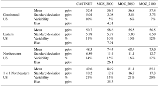
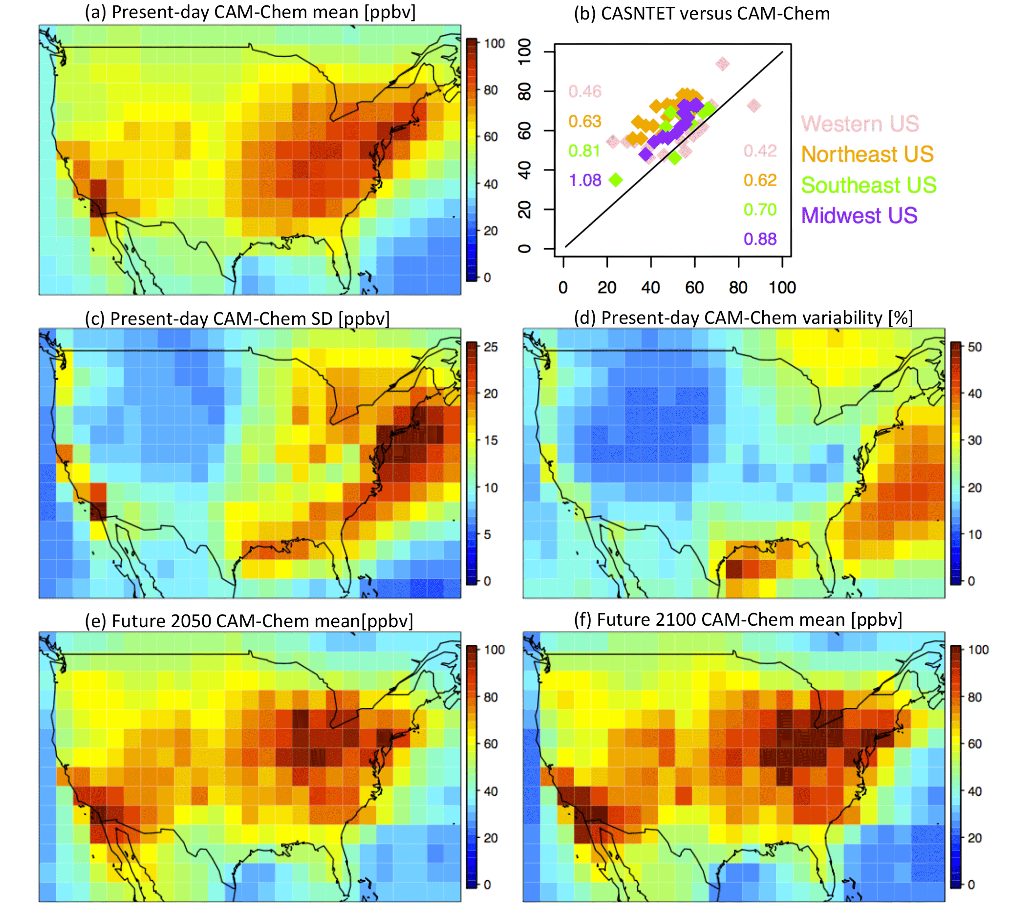
Figure 2Continental US surface maps of (a) present-day CAM-chem mean MDA8 O3, (b) CAM-Chem (y axis) comparison to CASTNET observations (x axis) for the year 2000 (see Brown-Steiner et al., 2018, for additional comparisons), (c) present-day CAM-chem standard deviation of MDA8 O3, (d) present-day CAM-chem variability (standard deviation divided by mean, as a percent), (e) future CAM-chem year-2050 mean MDA8 O3, and (f) future CAM-chem year-2100 mean MDA8 O3. All model results are averaged over every JJA day in the time series, while the CASTNET results are only for the year 2000. The numbers in (b) are slopes (left) and R2 values (right).
3.1 Spatial and temporal comparisons
Figure 2 compares summertime (JJA) maximum daily 8 h average ozone (MDA8 O3) from the present-day model simulation (MOZ_2000, Fig. 2a) to the year-2000 CASTNET observations (Fig. 2b). Figure 2c and d plot the MDA8 O3 standard deviation and variability for MOZ_2000, while Fig. 2d and e compare the mean summertime MDA8 O3 for the future simulations (MOZ_2050 and MOZ_2100). Some of the averaging strategies we present can average away the high ozone behavior this MDA8 O3 metric is intended to quantify, but it is such a well-reported metric that focusing our analysis on it allows for ready comparisons to other studies. The well-known high ozone bias in the eastern US (e.g., Lamarque et al., 2012; Travis et al., 2016; Barnes et al., 2016) is apparent, but otherwise the spatial variability over the entire continental US is well captured. While we do examine the magnitude of surface ozone in this paper, most of our analysis is focused on the variability around the mean value (the anomaly), and as we show below, the CASTNET observations and CESM results are largely consistent in their representation of ozone variability (Fig. 2, Table 1). The standard deviation of the simulated MDA8 O3 is large over the eastern US and the Pacific Coast, with peak values of ±25 ppbv over the highly populated Atlantic Coast (Fig. 2c). The variability (defined as the standard deviation divided by the mean, expressed as a percentage) is lowest over the western US (∼ 15 %), only slightly higher over the eastern US (up to 25 %), and highest (up to 50 %) over the coastal regions (Fig. 2d). We consider both the standard deviation (ppb) and a mean-normalized standard deviation (as a percentage). The normalized standard deviation allows for a more direct comparison of the shape of the MDA8 O3 distributions between the simulations and available observations, which accounts for the noted ozone biases (Fig. 2b, c and Table 1). The future climate simulations, MOZ_2050 and MOZ_2100 (Fig. 2e and f, respectively), although run with different parametric settings than MOZ_2000 (see Sect. 2), simulate a similar spatial distribution of surface ozone, although under the warmer simulated climate of 2050 and 2100. These future climate simulations have a similar spatial pattern to the present-day simulation (Fig. 2a), with high ozone levels in the eastern US that increase from 2050 to 2100 (see Garcia-Menendez et al., 2017, for more details).
Figure 3 compares box plots over the four telescoping regions (Fig. 1) for MOZ_2000, the CASTNET data, the detrended CASTNET data, and for the single year 2000 for the CASTNET data (Fig. 3a–d), and Table 1 summarizes relevant statistics. In order to compare CASTNET ozone to the simulated ozone, which does not have a trend over time, we detrend the CASTNET data in order to remove the impact of any temporal trends (e.g., NOx emissions reductions) on ozone. The northeastern US ozone bias is apparent at the smaller spatial scales (Fig. 3c, d) and is less apparent when averaging over larger regions (Fig. 3a, b). Figure 3e compares the year-to-year box plots of the JJA MDA8 O3 for the MOZ_2000 and the detrended CASTNET data and demonstrates the variability both in the median and spread of the ozone values in both the modeled and simulated data. While the MOZ_2000 ozone is generally higher than the CASTNET data, there are years in which the CASTNET data has higher ozone extremes. The red box plot in Fig. 3e, which corresponds to the red box plot in Fig. 3b, indicates that the year 2000 was an anomalously low year for observed ozone, although not the lowest.
While all the CESM CAM-chem simulations have high ozone biases in the northeastern US (Figs. 2 and 3, Table 1), their capability to simulate ozone variability is consistent with the available observations (for present day) and for expectations of ozone variability changes in the future climate (for MOZ_2050 and MOZ_2100). It is clear that variability increases when the size of the averaging region decreases – a fact that is well noted in the literature, as in Hawkins and Sutton (2012) for climate variables and Barnes et al. (2016) for ozone. As can be seen in Table 1, the CASTNET variability increases as the spatial scale decreases (10, 13, 16, and 20 % for our telescoping regions from continental to a single northeastern US grid box), and MOZ_2000 largely captures this trend, albeit with lower overall variability (5, 10, 15, and 15 %). This increase in ozone variability with decreasing spatial scale is maintained in the future climate simulations (6, 10, 16, and 21 % for MOZ_2050 and 7, 12, 17, and 20 % for MOZ_2100). Table S1 contains statistics for the other telescoping regions.
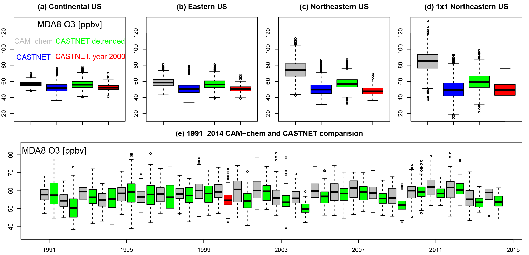
Figure 3(a–d): Box plots for surface MDA8 O3 for every summertime (JJA) day from 1991 to 2014 averaged over the continental US, the eastern US, the northeastern US, and a single grid cell in the northeastern US from CAM-chem (grey), CASTNET observations (blue), detrended CASTNET observations centered at the year 2000 (green), and, since the CAM-chem simulations have cycled year-2000 emissions and boundary conditions, the CASTNET values for the year 2000 only (red). (e) Comparison of the yearly JJA MDA8 O3 estimates averaged over the eastern US for CAM-chem (grey) and the detrended CASTNET (green) from 1991 to 2014. The single red box plot coincides with the red box plot in (b). The units are in ppbv and for each box plot the box contains the interquartile range (IQR); the horizontal line within the box is the median; and the whiskers extend out to the farthest point, which is within 1.5 times the IQR with circles indicating any outliers.
3.2 Variability, averaging windows, and thresholds
As we aim to quantify the potential tradeoffs that result from a particular choice of temporal and spatial scales on the assessment of ozone variability within the US, we represent the spatial scale by applying the telescoping regions (see Fig. 1 and Sect. 2.3) and we represent the temporal scale through the use of moving averaging windows (see Sect. 2.4). We frame much of the following analysis from the perspective of limited simulation length in order to approximate the question that decision-makers and modelers face when constrained by limited computational capabilities or available data: what is the likelihood that a particular estimate (of both the mean and the variability) is not a true representation of the true mean and variability but rather a product of the underlying variability at the particular choice of spatial and temporal scale?

Figure 4Comparisons of the variability represented by the summertime MDA8 O3 anomaly (from the long-term summertime mean) for the four datasets in this study (CASTNET, MOZ_2000, MOZ_2050, MOZ_2100, shown in columns) averaged over the four telescoping regions (the continental US, the eastern US, the northeastern US, and a single grid cell within the northeastern US). In each panel, the horizontal axis is the number of years in the dataset (24 years, 1991–2014, for CASTNET; 26 years, 1990–2015, for MOZ_2000; and 30 years, 2036–2065 and 2086–2115, for MOZ_2050 and MOZ_2100), and the vertical axis represents the length of the averaging window (ranging from 1 day, bottom row, up to the entire time series, top pixel, upper right corner of each triangle). Each pixel represents the estimate of the ozone anomaly for a given averaging window (vertical axis) ending at a given time (horizontal axis). Horizontal lines indicate the length of averaging window required to guarantee that the variability drops below thresholds of 5 ppbv (solid), 1 ppbv (dashed), and 0.5 ppbv (dotted).
Figure 4 presents this likelihood by plotting all possible estimates of MDA8 O3 (as anomalies from the long-term mean) over all possible selections of averaging window (from 1 day up to the complete time series) for our telescoping regions. The semi-cyclical and highly autocorrelated nature of surface ozone is apparent at all spatial scales, with alternating cycles of anomalously high and low ozone. The temporal impact of anomalous ozone events is indicated by the vertical and right-leaning diagonal striations, which show that anomalous ozone events can impact estimates of ozone values within averaging windows up to 15 or 20 years. Figure 4 demonstrates how small-scale anomalously high or low ozone values (that come only from meteorological variability) can impact temporal averages of 5, 10, or even 20 years. For instance, a selected 5-year averaging window within the MOZ_2000 simulation averaged over the northeastern US could be 2.5 ppbv higher or lower than the 25-year mean value of 74 ppbv, a potential error of 7 %. Horizontal lines in Fig. 4 mark the length of averaging windows that are needed to ensure that ozone anomaly for any selection of averaging window does not exceed a given threshold (5, 1, and 0.5 ppbv for solid, dashed, and dotted lines, respectively). This potential error is larger within smaller regions and at the shorter selections of the averaging window. While the high and low ozone anomalies differ in time between CASTNET, MOZ_2000, MOZ_2050, and MOZ_2100 in Fig. 4, the impact of spatial and temporal averaging is consistent.
We also quantify this variability in Figs. S1 and S2, which plots the likelihood (as a percentage) that a particular selection of spatial (rows) and temporal (x axis) scale estimates ozone values that exceed a particular threshold (colored lines) away from the true mean value. For instance, if we were interested in characterizing ozone behavior (e.g., estimating a trend, or the mean value) in the northeastern US, but were limited to a 5-year simulation, there is more than a 50 % likelihood that the simulated ozone is 1 ppbv away from the 26-year mean and an 80 % likelihood that the discrepancy is greater than 0.5 ppbv. However, these data indicate that there is a virtual certainty that the estimate will be within 2.5 ppbv of the true mean value. We should note that, at the grid-cell level and within a 10-year period, the surface ozone variability can exceed 1 ppbv but is unlikely to exceed 2.5 ppbv (Fig. 4) and that a 20-year trend is very likely to be able to identify significant ozone signals among the impact of meteorological variability on atmospheric chemistry. Our results also align with the results from Garcia-Menendez et al. (2017), which recommended that simulations need to be at least 15 years long to identify anthropogenically forced ozone signals on the order of 1 ppbv.
Figures 4, S1, and S2 compare the CASTNET observations to the three CESM CAM-chem simulations, and, while there are minor differences, there are broad features that are consistent. First, using longer temporal averaging windows reduces the influence of small-scale ozone variability at all spatial scales, and, depending on the acceptable threshold, one can select a temporal scale that effectively reduces the likelihood of exceeding that threshold to zero. Second, larger spatial scales also reduce this likelihood of exceeding a given threshold, but not as effectively as longer temporal scales. Finally, the impact of both temporal and spatial averaging on ozone variability is largely consistent for the CASTNET observations and for all three CESM CAM-chem simulations.

Figure 5Spatial plots over the continental US plotting the likelihood (%) that an estimate of ozone exceeds a given threshold due to meteorological variability (rows) at the grid-cell level when using different lengths of averaging windows (columns) for the present-day CESM simulation (MOZ_2000).
3.3 Selection of temporal averaging scales
Figure 5 extends this analysis to examine the spatial heterogeneity of this likelihood of the meteorological variability causing ozone anomalies exceeding particular thresholds at the grid-cell level. Here we plot four thresholds (0.5, 1, 2.5, and 5 ppbv) and four averaging windows (1, 5, 10, and 20 years) for the MOZ_2000 simulation. Ozone variability is highest in the eastern US. At the grid-cell level, there are two strategies for filtering out the noise associated with natural meteorological variability (and thus enhancing signal detection capabilities): either average over longer periods, or acknowledge the level of noise and increase the threshold. For these data, it is virtually certain that any 20-year average will be within 5 ppbv of a full 25-year mean value (which itself may not be an accurate representation of a longer simulation) and virtually certain that any 1-year average will be at least 0.5 ppbv away from the mean.

Figure 6As in Fig. 5, but only the second row (1 ppbv threshold), for present-day CAM-chem (MOZ_2000), future CAM-chem 2050 (MOZ_2050), and future CAM-chem 2100 (MOZ_2100).
Figure S3 extends the analysis of Fig. 5 by comparing the MOZ_2000, MOZ_2050, and MOZ_2100 simulations across the four thresholds for the 5-year averaging window. Figure 6 similarly compares the 1 ppbv ozone threshold across the four averaging windows for MOZ_2000, MOZ_2050, and MOZ_2100. Interpreting Figs. 6 and S3 gives largely consistent interpretations compared to the analysis above (Fig. 5) – namely, that at the grid-scale level increasing the temporal averaging window (Fig. 6) or increasing the acceptable ozone threshold (Fig. S3) is effective at reducing the impact of the meteorological variability on estimates of the ozone signal. Shorter windows (or smaller thresholds) are needed in the western US (where variability is smaller, see Fig. 2d) than in the eastern US (where variability is larger) as well as over coastal and highly populated regions. Finally, the 1 ppbv threshold and the 5-year averaging window plots (in either Figs. 5 and S3) indicate that the spatial distribution and location of the peak variability may shift into the future, although this may be due to parametric differences between MOZ_2000, MOZ_2050, and MOZ_2100. Future simulations will be needed to check this shift in peak ozone variability.
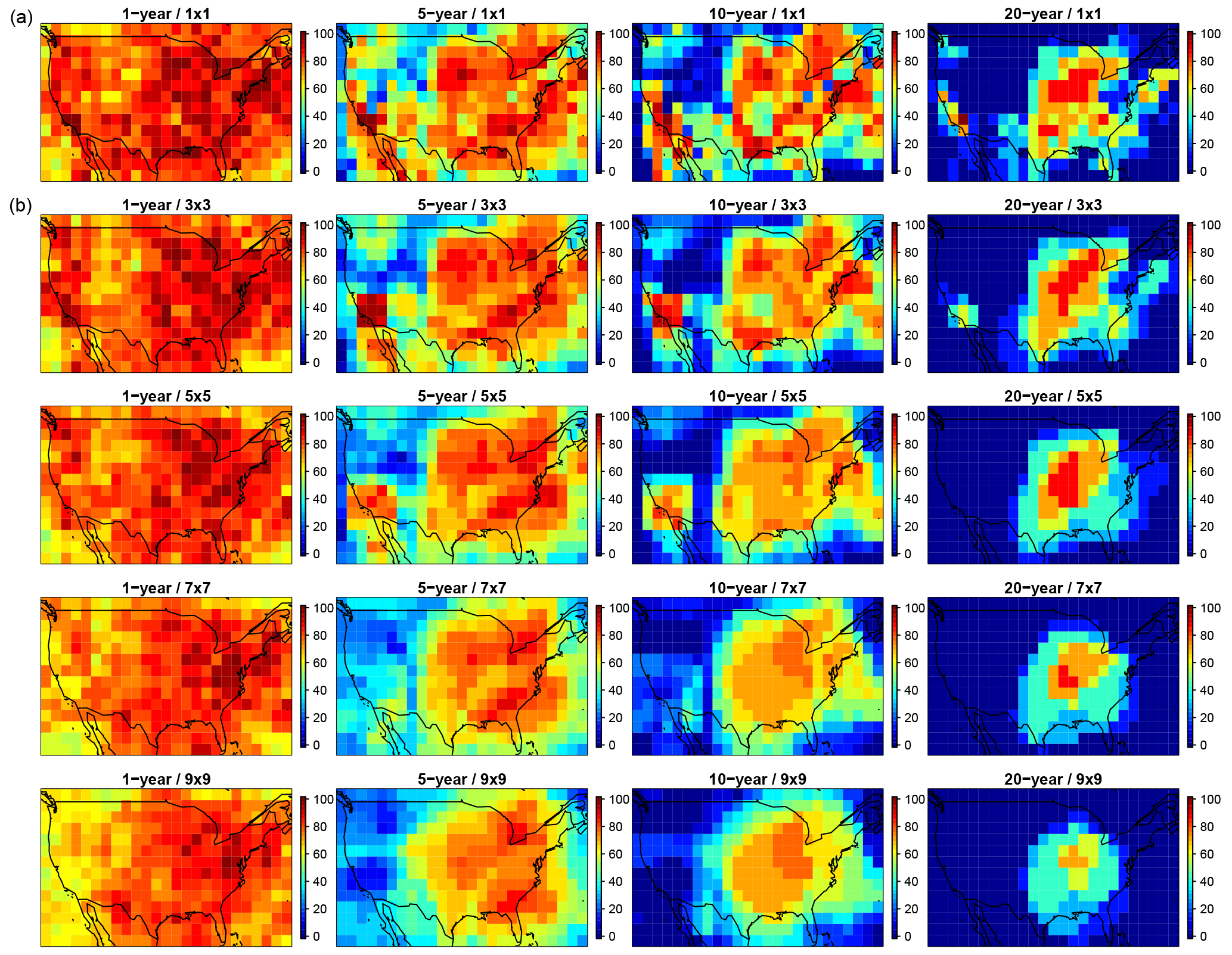
Figure 7Combined impact of temporal and spatial averaging on reducing ozone variability on the likelihood (%) of exceeding the 0.5 ppbv threshold (as in Figs. 5, 6, and S3) for the present-day MOZ_2000 simulation. The top row is the same as in Fig. 6, while the lower rows have averaged the values within a 3 × 3, 5 × 5, 7 × 7, and 9 × 9 grid box surrounding each individual grid cell.
3.4 Selection of spatial averaging scales
We examine the impact of increasing the spatial averaging region (Fig. 7) at four different temporal averaging windows (1, 5, 10, and 20 years) and for the smallest ozone threshold from the previous section (0.5 ppbv). It is evident that, at all temporal averaging windows, expanding the number of surrounding grid cells that are averaged together consistently decreases the likelihood of exceeding the 0.5 ppbv threshold, although these reductions are relatively small at the 1-year window, especially over the eastern US. While increasing the spatial averaging from a single grid cell up to include the surrounding 81 grid cells (bottom row in Fig. 7) manages to essentially smooth away much of the spatial heterogeneity in surface ozone (by moving down any column in Fig. 7); it does not eliminate the likelihood of exceeding the 0.5 ppbv threshold over much of the eastern US. For instance, even at a 20-year averaging window, and by averaging together the surrounding 81 grid cells over locations in the eastern US, there is still a 20–70 % likelihood of exceeding the 0.5 ppbv threshold due to the small-scale impact of the meteorological variability on atmospheric chemistry.
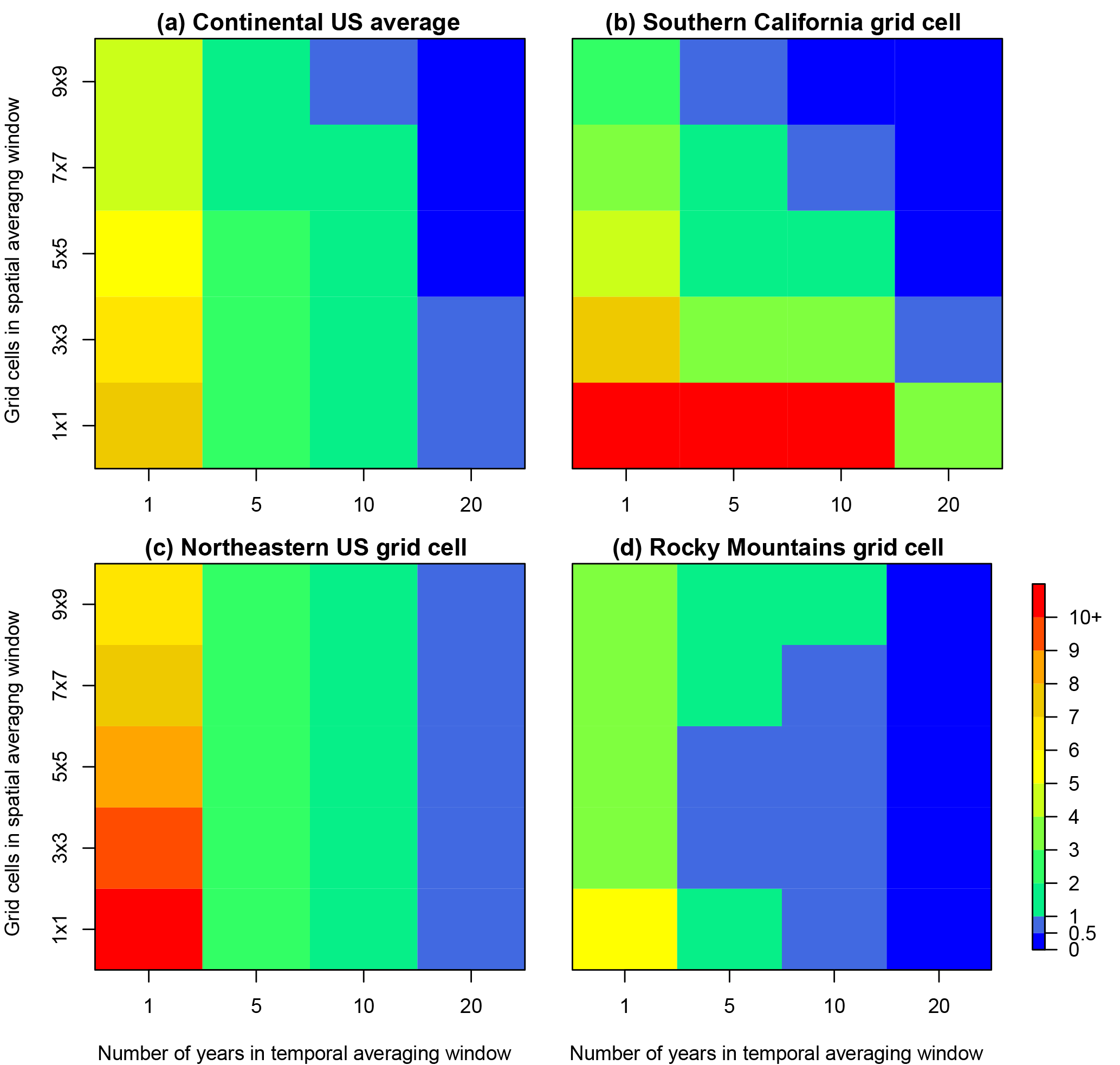
Figure 8The maximum potential calculated MDA8 O3 anomaly (ppbv) from the long-term mean for (a) the continental US average and three individual grid cells taken from (b) southern California, demonstrating effective temporal and spatial averaging; (c) the northeast, where spatial averaging is ineffective; and (d) the Rocky Mountains, where spatial averaging initially reduces the anomaly but then increases the anomaly as surrounding regions get included in the spatial average. The number of years included in the temporal averaging window increase along the x axis and the number of grid cells included in the spatial averaging window increase along the y axis. A full map of the continental US can be found in the Supplement (Fig. S4). Note that the color scale is nonlinear, and the color transitions are selected to match the thresholds established throughout this paper.
3.5 Combination of spatial and averaging scales
We now examine the combined impact of temporal and spatial averaging on reducing the influence of small-scale ozone variability in order to enhance ozone signal detection capabilities. Table S2 summarizes our analysis by dividing the likelihood of the ozone variability estimates exceeding selected thresholds away from the long-term mean into four categories: (1) the length of the averaging window over which ozone is averaged (columns), (2) the magnitude of the ozone threshold of interest (rows), (3) the observed (CASTNET) and modeled (MOZ_2000, MOZ_2050, and MOZ_2100) ozone data (sub-columns), and (4) the size of the spatial extent over which ozone is averaged (sub-rows). A graphical representation consistent with the data presented in Table S2 is plotted in Fig. 8 for the continental US average and for three grid cells that represent various cases. In each plot in Fig. 8, by moving along columns from left to right, we can see the influence of increasing the size of the temporal averaging window, and, by moving along rows (from the bottom to the top), we can see the influence of increasing the spatial averaging scale. By taking in the entire plot as a whole, we can get a feel for the combined influence of both temporal and spatial averaging. Figure S4 contains a plot for each grid cell in the continental US.
On average within the continental US, both temporal and spatial averaging are effective at reducing the calculated MDA8 O3 anomaly, although temporal averaging is more effective (Fig. 8a). There are many grid cells in the eastern and western US coasts (Fig. 8b and S4), where both spatial and temporal averaging are effective, but their combined usage is especially effective. There are also many grid cells where temporal averaging is effective but spatial averaging is barely effective or not effective at all (Figs. 8c and S4). Finally, there are some grid cells, particularly in the central US (Figs. 8d and S4), where spatial averaging over smaller regions is effective, but spatial averaging of larger regions actually increases the calculated MDA8 O3 anomaly by including surrounding grid cells that have higher variability.
We now return to the original four research questions posed in Section 1. First, what is the magnitude of ozone variability due to meteorology alone at the smallest scale and what is the impact of increasing the scale of temporal and spatial averaging? In both observed and modeled MDA8 O3 surface data, the small-scale variability driven solely by the meteorological variability impact on atmospheric chemistry (expressed as the standard deviation as a percentage of the mean) can exceed 20 % (Table 1, Fig. 2d). The chemical variability examined here is the result of fluctuations in meteorology, which itself results from larger-scale climatological drivers. While variability in emissions also influences atmospheric chemistry, our analysis has removed the influence of emissions variability and isolated the variability due to meteorology. A more comprehensive analysis of chemical variability will need to account for both meteorological and emission variability, which is complicated by temporal trends in both the emissions of ozone precursor species and the climate.
There is high temporal and spatial heterogeneity of surface ozone variability (Fig. 2d), with the lowest values found in the western US (< 10%), higher values found in the eastern US (up to 20 %), and the highest values found over coastal or heavily populated regions (up to 30 %). Averaging over longer temporal scales (by increasing the averaging window) and over larger spatial scales (by expanding the averaging region) can reduce the magnitude of the calculated variability, with temporal averaging proving to be more effective than spatial averaging in most cases (Fig. 8). In this study, we performed simple spatial averaging, but there are other methodologies for smoothing two-dimensional signals (e.g., Räisänen and Ylhäisi, 2011; Pogson and Smith, 2015) that could potentially increase signal detection capabilities.
Second, are there combinations of temporal and spatial averaging that maximize the filtration of calculated ozone variability and thus maximize the potential for signal detection? Figure 8 (and Fig. S4) demonstrates clearly that there are cases in which the combined usage of temporal and spatial averaging can reduce the calculated variability better than either strategy alone (see Fig. 8b), although there are many regions within the eastern US in which spatial averaging has little to no impact on reducing the calculated variability (Fig. 8c) or even results in an increase in the calculated variability (Fig. 8d). There are no such cases (see Fig. S4) in which expanding the temporal averaging scale increases the calculated ozone variability. This could potentially enable region-specific averaging strategies that help decision-makers identify and meet regional air quality objectives.
Third, are these results dependent on the particular parameterizations of the CESM CAM-chem model and are they consistent with the available CASTNET observations? The three CESM CAM-chem simulations exhibited consistent representations of ozone variability, consistent with our understanding of future changes to the climate (and meteorology) and the resulting impact on atmospheric chemistry (Table 1, Figs. 4, S1, and S2). Compared to the CASTNET observations (which we detrended to remove the influence of changing precursor emissions), the present-day simulation (MOZ_2000) exhibited a high ozone bias in the eastern US, while the representation of the ozone variability is comparable (Table 1).
Fourth, how may these strategies be applied to other datasets, be they chemical, meteorological, or climatological? Much of this analysis could be applied to any dataset that has spatial and temporal coverage, as long as some set of acceptable thresholds is provided. While our time step in this analysis is daily (given the MDA8 O3 metric), and applied only to summertime (JJA) days, any time step (i.e., hourly, monthly, annual, decadal) could be utilized as long as cyclical trends (e.g., diurnal or seasonal cycles) are removed. Indeed, the sliding-scale presentation in Figs. 8 and S4 can specifically be utilized to identify particular spatial and temporal scales that are sufficient to identify signals at particular thresholds and to identify particular geographic regions that are best suited to identify a given signal. For example, Sofen et al. (2016) identified regions across the globe where additional observations would be particularly suited to improve our understanding of surface ozone behavior, and our analysis could potentially be used to identify particular temporal and spatial averaging scales that could further maximize the capability for trend detection. In particular, Sofen et al. (2016) noted that the peak in the power spectrum of the El Niño–Southern Oscillation (ENSO) on surface ozone is at the 3.8-year timescale, and that, within some regions within the US, the amplitude of the ENSO influence on surface ozone approached 0.5 ppbv (and up to 1.1 ppbv globally). Our analysis shows that there are no grid cells within the continental US where a 0.5 ppbv signal can be identified at the 5-year (or shorter) temporal averaging scale (Fig. S4), but that there are many regions – especially within the western US – in which even a modest amount of spatial averaging can identify surface ozone signals below the 1 ppbv level with a 5-year or shorter averaging window. The type of sliding-scale analysis – in which spatial and temporal averaging are utilized individually and in combination – as presented in Figs. 8 and S4 could readily be applied to a wide range of atmospheric (and other) topics to aid in the capability to identify signals that exist both in space and in time. In particular, low-frequency oscillations (e.g., ENSO, and others) and other forms of internally or externally forced trends (e.g., anthropogenic and natural changes in emissions) are readily adaptable to this type of analysis, which could address signals pertaining to precipitation, biogenic emissions, boundary layer variables, cloud properties, and many others.
We did not quantify statistical significance (as in Lewandowsky et al., 2015) as our goals were to understand the general nature of ozone variability at all scales and for all signal strengths. Statistical significance testing (and other statistical techniques) can certainly provide additional information as to the strengths of ozone signals within the underlying variability and can be used to extend these results in a case-by-case manner, but we leave this testing to future studies that can focus on particular air quality objectives at particular temporal and spatial scales. Furthermore, future research examining the impact of spatial and temporal averaging using regional-scale models, models with different resolutions, and the inclusion of urban observations could provide additional insight into understanding chemical variability and averaging techniques.
Smaller signals require longer temporal averaging periods to identify. Figure 4 shows that a 0.5 ppb MDA8 O3 signal will emerge after 15–20 years of temporal averaging. The range here reflects different spatial averaging domains, with larger domains requiring shorter temporal averaging windows than smaller domains (i.e., 15 years for averaging over the continental US and 20 years for averaging over the northeastern US). This would mean that an average trend of 0.25–0.33 ppb year−1 would require a time series of at least 15 years to identify. Similarly, a 1.0 ppb MDA8 O3 signal emerges after 7–15 years, which indicates an average trend of 0.14–0.67 ppb year−1 would take at least 7 years to identify. Finally, a 5 ppb signal can be identified in less than 3 years, which indicates that an average trend of 1.67 ppb year−1 or greater would only require a 3-year time series. This presents particular difficulties if the ozone signal of interest is a trend spanning a time period on the same order. The 10–15 year averaging timescale we propose translates into a length of time beyond which you are likely to not see spurious trends above 0.5 ppb, but there are many cases in which the identification of a small trend is desired with less than 10–15 years of available data. For instance, Jiang et al. (2018) have found that NOx emissions reductions since 2005 are not as strong as previously expected, showing a significant slowdown beginning in 2011. This has large implications for ozone and for short-term decisions for air quality managers within the United States, who have to promulgate policies on short-term scales without the luxury of postponing action until longer and more complete datasets become available. As we have shown, spatial and temporal variability due to meteorology is high, and the identification and quantification of trends over 5, 10, or 15 years is difficult, particularly at small spatial scales.
However, as we have shown, a consideration of the impact on variability – and how variability changes over time – is often pivotal to understanding the nature of the signals being examined. In this paper, we have provided methods for quantifying the spatial and temporal variability and strategies for determining which types of signals are likely detectable at particular temporal and spatial scales. Some signals, especially small signals at small scales, are simply not large enough to emerge from the variability and thus may not be detectable without additional data or expanding the temporal and spatial averaging scales used for analysis. Quantifying the signal-to-noise ratio at a variety of spatial scales, and determining an acceptable threshold of a particular signal, could be one accessible method for providing this context. The risk in neglecting the quantification and contextualization of the magnitude of the ozone signal relative to the magnitude of the variability induced by the internal meteorology – and the impact of temporal and spatial averaging – is primarily the risk of drawing conclusions that are more sensitive to a particular peculiarity in the underlying variability rather than the signal itself.
We quantified the impact of spatial and temporal averaging at different scales – both individually and combined – on estimates of summertime surface ozone variability and the resulting likelihood of overconfidence in estimates of chemical signals over the United States using CASTNET observations and the CESM CAM-chem model. We simulate three multi-decadal time periods, each with constant surface emissions, and find that this analysis is consistent across our simulated time periods and that our results are not sensitive to particular configurations and parametric choices within the CESM CAM-chem (i.e., emissions, meteorology, and climate). We also provide a conceptual framework for gaining understanding of the influence of spatial and temporal averaging that may be adapted to a wide range of atmospheric and surface phenomena, provided sufficient spatial and temporal coverage. Here we focus on summertime surface ozone, a highly variable (in both space and time) atmospheric constituent with severe human health impacts and implications for planetary climate, which is the focus of many local, regional, and national policies. However, these ozone signals (e.g., temporal trends or regional averages) are frequently small when compared to the magnitude of the day-to-day ozone variability, and thus detecting these signals can be challenging. In particular, it would be impractical to delay interpreting observations for 10–15 years or alternatively to expand the spatial averaging such that small-scale features are smoothed away. Nonetheless, it is unwise to over-interpret trends and signals based on observations from a limited spatial area and over a short temporal period. Our analysis and conceptual framework presented here cannot solve this tension, but it does demonstrate some strategies which can allow for a selection of spatial and temporal averaging scales, and a consideration of the error threshold, that can aid in this signal detection on a case-by-case basis. Taking into account the complex interactions involving trends and variability between emissions, chemistry, meteorology, and climatology necessitates a variety of strategies. This work quantifies the impact of spatial and temporal averaging in signal detection, which can be used in conjunction with ensembles of simulations, statistical techniques, and other strategies to further our understanding of the chemical variability in our atmosphere.
In order to quantify the impact of spatial and temporal averaging on summertime ozone variability, we start by selecting four telescoping spatial regions (the continental US, the eastern US, the northeastern US, and a single grid cell within the northeastern US) and examine all possible choices for averaging windows (ranging from daily to multi-decadal windows), although we focused primarily on averaging windows of 1, 5, 10, and 20 years. We find that – consistent with previous studies – summertime MDA8 O3 variability is largest at the smallest spatial and temporal scales and is frequently on the order of ±10–20 ppbv or which is roughly 15–20 % of the mean ozone signal. In order to minimize the chemical noise that results from meteorological variability – and thus enhance the signal – we find averaging windows of 10–15 years (and sometimes longer at the smaller spatial scales) combined with modest (nearest-neighbor) spatial averaging substantially improve the capability for signal detection. For signals that are large compared to the underlying meteorological variability (e.g., strong emissions reductions), shorter averaging windows and smaller spatial regions may be used. We recognize that achieving a 10–15 year temporal averaging window is difficult, but this recommendation is consistent with recent literature (e.g., Barnes et al., 2016; Garcia-Menendez et al., 2017). For studies where 10–15 years of averaging is impractical, we recommend that some spatial and temporal context is provided that demonstrates that the signals being examined are robust and not the result of internal variability or noise. We also recognize that our analysis is just one strategy for enhancing signal detection capabilities and will ideally be used alongside others, such as perturbed initial condition ensembles, running simulations with either internal or forced meteorology, and examining a region or time period with different models or parameterizations.
We show that the largest summertime ozone variability is found in the eastern US (Figs. 5 and S4), and subsequently there are many regions within the eastern US where even a 20-year averaging window has a non-negligible likelihood of estimating ozone variability that is dependent (with possible error in the 1–3 ppbv range) on the particular years selected. In addition, over much of the eastern US, simulations of 5 years or less have a substantial likelihood (40–90 %, Figs. S1 and S2) of reflecting the influence of meteorological variability on chemistry rather than the mean state of surface ozone, with the possibility of 5–10 ppbv error (Fig. S4). While we have detrended the CASTNET observations to compare to the constant year-2000 cycled emissions in the simulations, the CASTNET time series inherently includes the compounded variability of both meteorological and emission sources. Future studies will need to expand this analysis to include trends and variability in the emissions, as well as in the meteorology.
Finally, we demonstrate a conceptual framework that allows for a sliding-scale view of surface ozone variability, in which both temporal and spatial averaging is examined at every grid cell within the continental US. We show that the magnitude of estimates of ozone variability can be reduced with both temporal and spatial averaging, although temporal averaging tends to be more effective. While there are many regions in which both temporal and spatial averaging used in conjunction substantially reduce the estimate of ozone variability, there are some regions where spatial averaging is ineffective or even counter-effective. In contrast, this is not the case for temporal averaging, which consistently reduces the magnitude of estimated ozone variability. Our analysis could be combined with other studies (e.g., Sofen et al., 2016) to guide observational and modeling strategies and identify regions and scales at which particular signals are most likely to be identified.
The CESM CAM-Chem code is available through the National Center for Atmospheric Research/University Corporation for Atmospheric Research (NCAR/UCAR) website (http://www.cesm.ucar.edu/models/cesm1.2/, last access: 7 June 2018), and this project made no code modifications from the released model version.
The raw model output is archived on the NCAR servers, and processed data are archived at https://dspace.mit.edu/handle/1721.1/114467, last access: 7 June 2018.
The supplement related to this article is available online at: https://doi.org/10.5194/acp-18-8373-2018-supplement.
BBS ran the present-day simulation, analyzed the data, and wrote the manuscript. EM ran the future climate simulations, while FGM ran the future atmospheric chemistry simulations and made the data available to BBS. NS, RP, EM, ST, and LE guided and reviewed the scientific modeling and analysis process. All authors provided feedback throughout the project and development of the manuscript.
The authors declare that they have no conflict of interest.
This model development work was supported by the U.S. Department of Energy
(DOE) grant DE-FG02-94ER61937 to the MIT Joint Program on the Science and
Policy of Global Change. Computational resources for this project were
provided by DOE and a consortium of other government, industry, and
foundation sponsors of the Joint Program. For a complete list of sponsors,
see http://globalchange.mit.edu (last access: 7 June 2018). Additional computing
resources were provided by the Climate Simulation Laboratory at NCAR's
Computational and Information Systems Laboratory (CISL), sponsored by the
National Science Foundation and other agencies. The National Center for
Atmospheric Research is funded by the National Science Foundation. The
authors would also like to thank Daniel Rothenberg for efficient processing
of the ozone files.
Edited by: Jayanarayanan Kuttippurath
Reviewed by: two anonymous referees
Angélil, O., Stone, D., Perkins-Kirkpatrick, S., Alexander, L. V., Wehner, M., Shiogama, H., Wolski, P., Ciavarella, A., and Christidis, N.: On the nonlinearity of spatial scales in extreme weather attribution statements, Clim. Dynam., 50, 2739–2752, 2017.
Barnes, E. A., Fiore, A. M., and Horowitz, L. W.: Detection of trends in surface ozone in the presence of climate variability, J. Geophys. Res.-Atmos., 121, 6112–6129, 2016.
Brown-Steiner, B., Hess, P. G., and Lin, M. Y.: On the capabilities and limitations of GCCM simulations of summertime regional air quality: A diagnostic analysis of ozone and temperature simulations in the US using CESM CAM-chem, Atmos. Environ., 101, 134–148, 2015.
Brown-Steiner, B., Selin, N. E., Prinn, R., Tilmes, S., Emmons, L., Lamarque, J.-F., and Cameron-Smith, P.: Evaluating Simplified Chemical Mechanisms within Present-Day Simulations of CESM Version 1.2 CAM-chem (CAM4): MOZART-4 vs. Reduced Hydrocarbon vs. Super-Fast Chemistry, Geosci. Model Dev. Discuss., https://doi.org/10.5194/gmd-2018-16, in review, 2018.
Camalier, L., Cox, W., and Dolwick, P.: The effects of meteorology on ozone in urban areaas and their use in assessing ozone trends, Atmos. Environ., 41, 7127–7137, 2007.
Cooper, O. R., Gao, R. S., Tarasick, D., Leblanc, T., and Sweeney, C.: Long-term ozone trends at rural ozone monitoring sites across the United States, 1990–2010, J. Geophys. Res., 117, D22307, https://doi.org/10.1029/2012JD018261, 2012.
de Elía, R., Biner, S., and Frigon, A.: Interannual variability and expected regional climate change over North America, Clim. Dynam., 41, 1245–1267, https://doi.org/10.1007/s00382-013-1717-9, 2013.
Deser, C., Phillips, A., Bourdette, V., and Teng, H.: Uncertainty in climate change projections: the role of internal variability, Clim. Dynam., 38, 527–546, https://doi.org/10.1007/s00382-010-0977-x, 2012.
Emmons, L. K., Walters, S., Hess, P. G., Lamarque, J.-F., Pfister, G. G., Fillmore, D., Granier, C., Guenther, A., Kinnison, D., Laepple, T., Orlando, J., Tie, X., Tyndall, G., Wiedinmyer, C., Baughcum, S. L., and Kloster, S.: Description and evaluation of the Model for Ozone and Related chemical Tracers, version 4 (MOZART-4), Geosci. Model Dev., 3, 43–67, https://doi.org/10.5194/gmd-3-43-2010, 2010.
Fiore, A. M., Jacob, D. J., Liu, H., Yantosca, R. M., Fairlie, T. D., and Li, Q.: Variability in surface ozone background over the United States: Implications for air quality policy, J. Geophys. Res.-Atmos., 108, 4787, 2003.
Fiore, A. M., Oberman, J. T., Lin, M. Y., Zhang, L., Clifton, O. E., Jacob, D. J., Naik, V., Horowitz, L. W., Pinto, J. P., and Milly, G. P.: Estimating North American background ozone in U.S. surface air with two independent global models: Variability, uncertainties, and recommendations, Atmos. Environ., 96, 284–300, 2014.
Frost, G. J., McKeen, S. A., Trainer, M., Ryerson, T. B., Neuman, J. A., Roberts, J. M., Swanson, A., Holloway, J. S., Sueper, D. T., Fortin, T., Parrish, D. D., Fehsenfeld, F. C., Flocke, F., Peckham, S. E., Grell, G. A., Kowal, D., Cartwright, J., Auerback, N., and Habermann, T.: Effects of changing power plant NOx emissions on ozone in the eastern United States: Proof of concept. J. Geophys. Res., 111, D12306, https://doi.org/10.1029/2005JD006354, 2006.
Garcia-Menendez, F., Saari, R. K., Monier, E., and Selin, N. E.: U.S. Air Quality and Health Benefits from Avoided Climate Change under Greenhouse Gas Mitigation, Environ. Sci. Technol., 49, 7580–7588, 2015.
Garcia-Menendez, F., Monier, E., and Selin, N. E.: The role of natural variability in projections of climate change impacts on U.S. ozone pollution, Geophys. Res. Lett., 44, 2911–2921, 2017.
Giorgi, F. and Bi, X.: Time of emergence (TOE) of GHG-forced precipitation change hot-spots, Geophys. Res. Lett., 36, L06709, https://doi.org/10.1029/2009GL037593, 2009.
Guenther, A. B., Jiang, X., Heald, C. L., Sakulyanontvittaya, T., Duhl, T., Emmons, L. K., and Wang, X.: The Model of Emissions of Gases and Aerosols from Nature version 2.1 (MEGAN2.1): an extended and updated framework for modeling biogenic emissions, Geosci. Model Dev., 5, 1471–1492, https://doi.org/10.5194/gmd-5-1471-2012, 2012.
Hawkins, E. and Sutton, R.: Time of emergence of climate signals, Geophys. Res. Lett., 39, L01702, https://doi.org/10.1029/2011GL050087, 2012.
Jacob, D. J. and Winner, D. A.: Effect of climate change on air quality, Atmos. Environ, 43, 51–63, 2009.
Jhun, I., Coull, B. A., Schwartz, J., Hubbell, B., and Koutrakis, P.: The impact of weather changes on air quality and health in the United States in 1994–2012, Environ. Res. Lett., 10, 084009, https://doi.org/10.1088/1748-9326/10/8/084009, 2015.
Jiang, Z., McDonald, B. C., Worden, H., Worden, J. R., Miyazaki, K., Qu, Z., Henze, D. K., Jones, D. B. A., Arellano, A. F., Fischer, E. V., Zhu, K., and Boersma, F.: Unexpected slowdown of US pollutant emission reduction in the past decade, P. Natl. Acad. Sci. USA, 115, 5099–5104, https://doi.org/10.1073/pnas.1801191115, 2018.
Kay, J. E., Deser, C., Phillips, A., Mai, A., Hannay, C., Strand, G., Arblaster, J. M., Bates, S. C., Danabasoglu, G., Edwards, J., Holland, M., Kushner, P., Lamarque, J.-F., Lawrence, D., Lindsay, K., Middleton, A., Munoz, E., Neale, R., Oleson, K., Polvani, L., and Vertenstein, M.: The Community Earth System Model (CESM) large ensemble project: A community resource for studying climate change in the presence of internal climate variability, B. Am. Meteorol. Soc., 96, 1333–1349, 2015.
King, A. D., Donat, M. G., Fischer, E. M., Hawkins, E., Alexander, L. V, Karoly, D. J., Dittus, A. J., Lweis, S. C., and Perkins, S. E.: The timing of anthropogenic emergence in simulated climate extremes, Environ. Res. Lett., 10, 094015, https://doi.org/10.1088/1748-9326/10/9/094015, 2015.
Knutti, R.: The end of model democracy?, Clim. Change, 102, 395–404, 2010.
Lamarque, J.-F., Emmons, L. K., Hess, P. G., Kinnison, D. E., Tilmes, S., Vitt, F., Heald, C. L., Holland, E. A., Lauritzen, P. H., Neu, J., Orlando, J. J., Rasch, P. J., and Tyndall, G. K.: CAM-chem: description and evaluation of interactive atmospheric chemistry in the Community Earth System Model, Geosci. Model Dev., 5, 369–411, https://doi.org/10.5194/gmd-5-369-2012, 2012.
Lamarque, J.-F., Dentener, F., McConnell, J., Ro, C.-U., Shaw, M., Vet, R., Bergmann, D., Cameron-Smith, P., Dalsoren, S., Doherty, R., Faluvegi, G., Ghan, S. J., Josse, B., Lee, Y. H., MacKenzie, I. A., Plummer, D., Shindell, D. T., Skeie, R. B., Stevenson, D. S., Strode, S., Zeng, G., Curran, M., Dahl-Jensen, D., Das, S., Fritzsche, D., and Nolan, M.: Multi-model mean nitrogen and sulfur deposition from the Atmospheric Chemistry and Climate Model Intercomparison Project (ACCMIP): evaluation of historical and projected future changes, Atmos. Chem. Phys., 13, 7997–8018, https://doi.org/10.5194/acp-13-7997-2013, 2013.
Lawrence, M. G., Hov, Ø., Beekmann, M., Brandt, J., Elbern, H., Eskes, H., Feichter, H., and Takigawa, M.: The chemical weather, Environ. Chem, 2, 6–8, 2005.
Lewandowsky, S., Risbey, J. S., and Oreskes, N.: On the definition and identifiability of the alleged “hiatus” in global warming, Sci. Rep., 5, 16784, 13 pp., 2015.
Lin, M., Horowitz, L. W., Oltmans, S. J., Fiore, A. M., and Fan, S.: Tropospheric ozone trends at Mauna Loa Observatory tied to decadal climate variability, Nat. Geosci., 7, 136–143, 2014.
McComiskey, A. and Feingold, G.: The scale problem in quantifying aerosol indirect effects, Atmos. Chem. Phys., 12, 1031–1049, https://doi.org/10.5194/acp-12-1031-2012, 2012.
Medhaug, I., Stolpe, M. B., Fischer, E. M., and Knutti, R.: Reconciling controversies about the `global warming hiatus, Nature, 545, 41–47, 2017.
Möller, D.: Chemistry of the Climate System, 331–334, Walter de Gruyter GmbH and Co., KG, Berlin/New York, 2010.
Monier, E., Scott, J. R., Sokolov, A. P., Forest, C. E., and Schlosser, C. A.: An integrated assessment modeling framework for uncertainty studies in global and regional climate change: the MIT IGSM-CAM (version 1.0), Geosci. Model Dev., 6, 2063–2085, https://doi.org/10.5194/gmd-6-2063-2013, 2013.
Monier, E., Gao, X., Scott, J. R., Sokolov, A. P., and Schlosser, C. A.: A framework for modeling uncertainty in regional climate change, Clim. Change, 131, 51–66, 2015.
Monier, E., Xu, L., and Snyder, R.: Uncertainty in future agro-climate projections in the United States and benefits of greenhouse gas mitigation, Environ. Res. Lett., 11, 055001, https://doi.org/10.1088/1748-9326/11/5/055001, 2016.
Phalitnonkiat, P., Sun, W., Grigoriu, M. D., Hess ,P., and Samorodnitsky, G.: Extreme ozone events: Tail behavior of the surface ozone distribution over the U.S., Atmos. Environ., 128, 134–146, https://doi.org/10.1016/j.atmosenv.2015.12.047, 2016.
Pogson, M. and Smith, P.: Effect of spatial data resolution on uncertainty, Environ. Model. Softw., 63, 87–96, 2015.
Pyle, J. A. and Zavody, A. M.: The modelling problems associated with spatial averaging, Q. J. Roy. Meteorol. Soc., 116, 753–766, 1990.
Räisänen, J. and Ylhäisi, J. S.: How much should climate model output be smoothed in space?, J. Climate, 24, 867–880, 2011.
Rasmussen, D. J., Fiore, A. M., Naik, V., Horowitz, L. W., McGinnis, S. J., and Schultz, M. G.: Surface ozone-temperature relationships in the eastern US: A monthly climatology for evaluating chemistry-climate models, Atmos. Environ., 47, 142–153, 2012.
Rienecker, M. M., Suarez, M. J., Gelaro, R., Todling, R., Bacmeister, J., Liu, R., Bosilovich, M. G., Schubert, S. D., Takacs, L., Kim, G-K, Bloom, S., Chen, J., Collins, D., Conaty, A., da Silva, A., Gu, W., Joiner, J., Koster, R. D., Lucchesi, R., Molod, A., Owens, T., Pawson, S., Pegion, P., Redder, C. R., Reichle, R., Robertson, F. R., Ruddick, A. G., Sienkiewicz, M., and Woollen, J.: MERRA: NASA's Modern-Era Retrospective analysis for Research and Applications, J. Climate, 24, 3624–3648, 2011.
Roberts, C. D., Palmer, M. D., McNeall, D., and Collins, M.: Quantifying the likelihood of a continued hiatus in global warming, Nat. Clim. Change, 5, 337–342, 2015.
Schnell, J. L. and Prather, M. J.: Co-occurrence of extremes in surface ozone, particulate matter, and temperature over eastern North America, P. Natl. Acad. Sci. USA, 114, 11, 2854–2859, 2017.
Schurer, A. P., Hegerl, G. C., Mann, M. E., Tett, S. F. B., and Phipps, S. J.: Separating forced from chaotic climate variability over the past millennium, J. Climate, 26, 6954–6973, 2013.
Searle, K. R., Chipperfield, M. P., Bekki, S., and Pyle, J. A.: The impact of spatial averaging on calculated polar ozone loss: 2. Theoretical analysis, J. Geophys. Res, 103, 25409–25416, 1998.
Sofen, E. D., Bowdalo, D., and Evans, M. J.: How to most effectively expand the global surface ozone observing network, Atmos. Chem. Phys., 16, 1445–1457, https://doi.org/10.5194/acp-16-1445-2016, 2016.
Stevenson, D. S., Young, P. J., Naik, V., Lamarque, J.-F., Shindell, D. T., Voulgarakis, A., Skeie, R. B., Dalsoren, S. B., Myhre, G., Berntsen, T. K., Folberth, G. A., Rumbold, S. T., Collins, W. J., MacKenzie, I. A., Doherty, R. M., Zeng, G., van Noije, T. P. C., Strunk, A., Bergmann, D., Cameron-Smith, P., Plummer, D. A., Strode, S. A., Horowitz, L., Lee, Y. H., Szopa, S., Sudo, K., Nagashima, T., Josse, B., Cionni, I., Righi, M., Eyring, V., Conley, A., Bowman, K. W., Wild, O., and Archibald, A.: Tropospheric ozone changes, radiative forcing and attribution to emissions in the Atmospheric Chemistry and Climate Model Intercomparison Project (ACCMIP), Atmos. Chem. Phys., 13, 3063–3085, https://doi.org/10.5194/acp-13-3063-2013, 2013.
Strode, S. A. and Pawson, S.: Detection of carbon monoxide trends in the presence of interannual variability, J. Geophys. Res.-Atmos., 118, 12257–12273, 2013.
Sun, J., Fu, J. S., Drake, J., Lamarque, J.-F., Tilmes, S., and Vitt, F.: Improvement of the prediction of surface ozone concentration over conterminous U.S. by a computationally efficient second-order Rosenbrock solver in CAM4-Chem, J. Adv. Model Earth. Sy., 9, 482–500, 2017.
Tilmes, S., Lamarque, J.-F., Emmons, L. K., Conley, A., Schultz, M. G., Saunois, M., Thouret, V., Thompson, A. M., Oltmans, S. J., Johnson, B., and Tarasick, D.: Technical Note: Ozonesonde climatology between 1995 and 2011: description, evaluation and applications, Atmos. Chem. Phys., 12, 7475–7497, https://doi.org/10.5194/acp-12-7475-2012, 2012.
Tilmes, S., Lamarque, J.-F., Emmons, L. K., Kinnison, D. E., Ma, P.-L., Liu, X., Ghan, S., Bardeen, C., Arnold, S., Deeter, M., Vitt, F., Ryerson, T., Elkins, J. W., Moore, F., Spackman, J. R., and Val Martin, M.: Description and evaluation of tropospheric chemistry and aerosols in the Community Earth System Model (CESM1.2), Geosci. Model Dev., 8, 1395–1426, https://doi.org/10.5194/gmd-8-1395-2015, 2015.
Tilmes, S., Lamarque, J.-F., Emmons, L. K., Kinnison, D. E., Marsh, D., Garcia, R. R., Smith, A. K., Neely, R. R., Conley, A., Vitt, F., Val Martin, M., Tanimoto, H., Simpson, I., Blake, D. R., and Blake, N.: Representation of the Community Earth System Model (CESM1) CAM4-chem within the Chemistry-Climate Model Initiative (CCMI), Geosci. Model Dev., 9, 1853–1890, https://doi.org/10.5194/gmd-9-1853-2016, 2016.
Travis, K. R., Jacob, D. J., Fisher, J. A., Kim, P. S., Marais, E. A., Zhu, L., Yu, K., Miller, C. C., Yantosca, R. M., Sulprizio, M. P., Thompson, A. M., Wennberg, P. O., Crounse, J. D., St. Clair, J. M., Cohen, R. C., Laughner, J. L., Dibb, J. E., Hall, S. R., Ullmann, K., Wolfe, G. M., Pollack, I. B., Peischl, J., Neuman, J. A., and Zhou, X.: Why do models overestimate surface ozone in the Southeast United States?, Atmos. Chem. Phys., 16, 13561–13577, https://doi.org/10.5194/acp-16-13561-2016, 2016.
US EPA: National Ambient Air Quality Standards for Ozone: Final Rule, Fed. Regist., 80, 65292–65468, 2015.
US EPA: CASTNET 2014 Annual Report Prepared by Environmental Engineering and Measurement Services, Inc. for the U.S. Environmental Protection Agency, 2016.
Weatherhead, E. C., Stevermer, A. J., and Schwartz, B. E., Detecting environmental changes and trends, Phys. Chem. Earth, 27, 399–403, 2002.
Wild, O. and Prather, M. J.: Global tropospheric ozone modeling: Quantifying errors due to grid resolution, J. Geophys. Res., 111, D11305, https://doi.org/10.1029/2005JD006605, 2006.
Young, P. J., Archibald, A. T., Bowman, K. W., Lamarque, J.-F., Naik, V., Stevenson, D. S., Tilmes, S., Voulgarakis, A., Wild, O., Bergmann, D., Cameron-Smith, P., Cionni, I., Collins, W. J., Dalsøren, S. B., Doherty, R. M., Eyring, V., Faluvegi, G., Horowitz, L. W., Josse, B., Lee, Y. H., MacKenzie, I. A., Nagashima, T., Plummer, D. A., Righi, M., Rumbold, S. T., Skeie, R. B., Shindell, D. T., Strode, S. A., Sudo, K., Szopa, S., and Zeng, G.: Pre-industrial to end 21st century projections of tropospheric ozone from the Atmospheric Chemistry and Climate Model Intercomparison Project (ACCMIP), Atmos. Chem. Phys., 13, 2063–2090, https://doi.org/10.5194/acp-13-2063-2013, 2013.