2.1 Filtering of KWs by 3-D normal-mode function expansion

The basic assumption behind the NMF expansion is that a global state of the atmosphere described by its mass and wind variables at any time can be considered as a superposition of the linear wave solutions upon a predefined background state. The NMF decomposition derived by Kasahara and Puri (1981) uses the σ vertical coordinate and linearization around the state of rest and realistic vertical temperature and stability stratification. The 3-D wave solutions of linearized primitive equations are represented as a truncated time series of the Hough harmonic oscillations and the vertical structure functions. The assumption of separability leads to separate equations for the vertical structure and horizontal oscillations. The latter are known as shallow-water equations on the sphere or Laplace tidal equations without forcing. The two systems are coupled by a separation parameter D which is called the equivalent height (Boyd, 2018). Eigenmodes of the global shallow-water equations are known as Hough harmonics. They describe two types of wave motions: Rossby waves and inertio-gravity waves which obey their corresponding dispersion relationships on the spherical Earth.

The expansion of a global input data vector $\mathit{X}(\mathit{\lambda },\mathit{\phi },\mathit{\sigma })=(u,v,h{)}^T$ can be represented by a discrete finite series as

The input data vector contains wind components u,v and the transformed geopotential height h defined as $h=g^{-\mathrm{1}}P$, where g is the gravity and P is defined as $P=\mathrm{\Phi }+R{T}_{\mathrm{0}}\ln \left(p_{\mathrm{s}}\right)$; that is, it is the sum of geopotential Φ and a surface pressure, p_s, term. Two other variables represent the specific gas constant for dry air (R) and the globally-averaged vertical temperature profile (T₀(σ)). The zonal and vertical truncations (K and M, respectively) define maximal numbers of zonal waves at a single latitude (wavenumber k) and a maximal number of vertical modes (denoted m), respectively. For every vertical structure eigenfunctions G_m(σ), Hough harmonic functions, ${\mathbf{H}}_{\mathrm{n}}^k(\mathit{\lambda },\mathit{\phi })$, describe non-dimensional oscillations in the horizontal plane of the fluid with the mean depth equal the equivalent depth D_m. The parameter D_m appears in Eq. (2) in the diagonal matrix S_m with elements (gD_m)^1∕2, (gD_m)^1∕2 and D_m, which normalizes the input data vector after the vertical projection and thereby removes dimensions. Parameter R is the total number of meridional modes which is a sum of the eastward inertio-gravity waves (EIG), westward inertio-gravity waves (WIG) and Rossby waves. Linearization about the state of rest is not a drawback of the method as wave frequencies are used solely for the formulation of the projection basis and not for studying wave propagation properties. As shown by Kasahara (1980) (see also its Corrigendum) the meridional structures of the Hough functions for large scales are not significantly different if the linearization is performed around the non-zero mean zonal flow. The impact of latitudinal shear on the KWs was shown to be negligible by Boyd (1978). Further details of the NMF projection procedure are given in Žagar et al. (2015).

For each zonal wavenumber, the Kelvin mode is the lowest eastward-propagating latitudinal Hough function. In Eq. (2), the KW is represented by the non-dimensional complex expansion coefficients ${\mathit{\chi }}_{\mathrm{n}}^k\left(m\right)$ with the meridional index n=1. However, to follow often-used notation, we shall denote the KW in the remainder of this study as the n=0 EIG mode, i.e. the KW wind and geopotential height are represented by coefficients ${\mathit{\chi }}_{\mathrm{kw}}={\mathit{\chi }}_{\mathrm{0}}^k\left(m\right)$. The truncation values are K=85 and M=60. This means that the KW signal in 3-D circulation at a single time instant consists of 5100 waves, 85 waves in every shallow-water equation system. Higher vertical modes were left out as their equivalent depth is smaller than 2 m and their contribution to the total KW signal is negligible in the outputs in the TTL and the stratosphere. The relation between the truncation parameters and the normal-mode projection quality is discussed in Žagar et al. (2015) and references therein.

Once the forward projection is carried out and coefficients ${\mathit{\chi }}_{\mathrm{n}}^k\left(m\right)$ are produced, filtering of KWs in physical space can be performed through Eq. (2) after setting all χ, except those representing the KWs, to zero. The result of filtering are fields u_kw, v_kw and h_kw, which provide the KW zonal wind, meridional wind and geopotential height perturbations. Notice here that in contrast to the equatorial β-plane, KWs on the sphere have a small meridional wind component which is thus left out from the discussion (Boyd, 2018).

The KW temperature perturbation, T_kw, can be derived from the h_kw fields on σ levels using the hydrostatic relation in σ coordinates:

The orthogonality of the normal-mode basis functions provides KW energy as a function of the zonal wavenumber and vertical mode. After the forward projection, the energy spectrum of total (potential and kinetic) energy for each KW can be computed using the energy product for the kth and mth normal modes (Žagar et al., 2015) as

The units are J kg⁻¹. The KW global energy spectrum as a function of the zonal wavenumber is obtained by summing energy in all vertical modes:

2.2 Examples of 3-D structure of KWs in L91 analyses

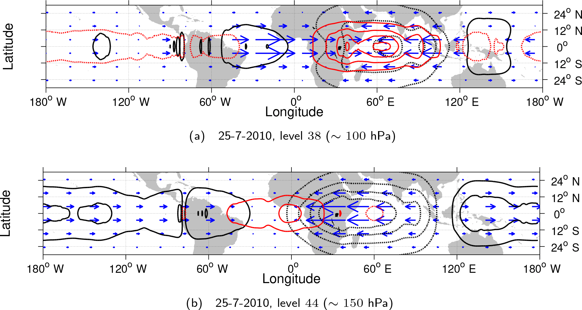
Figure 1The horizontal structure of KWs in the ECMWF analysis data on 25 July 2010 at (a) 100 and (b) 150 hPa. The geopotential height perturbations (h_kw) are shown by black contours, every 20 m, whereas temperature perturbations (T_kw) are coloured red (every 1 K). Dashed contours represent negative and full line contour positive perturbations. Zero lines are omitted.

Download

KWs are shown in Figs. 1–2 for a few days in July 2010 to introduce and illustrate their properties as filtered by the NMF methodology.

Figure 1 illustrates the meridional structure of KWs on 25 July 2010 on 2 levels. KW activity was found largest in the zonal wind component at 150 hPa over the Indian Ocean. The geopotential dipole structure is centred over the convective hotspot over the Maritime Continent. At 100 hPa, we find the largest amplitude of KW temperature perturbations up to 4 K positioned above the zonal wind maxima at 150 hPa. The meridional wind component of the KW is non-zero in spherical coordinates, but is at most 0.22 m s⁻¹ at 100 hPa, which is negligible compared to the zonal wind component (maximum 12.5 m s⁻¹) making the KW wind field primarily zonal. Note that the presented horizontal structure at a single level is a superposition of 60 vertical modes, i.e. 60 shallow water models with equivalent depths from about 10 km to a couple of metres.

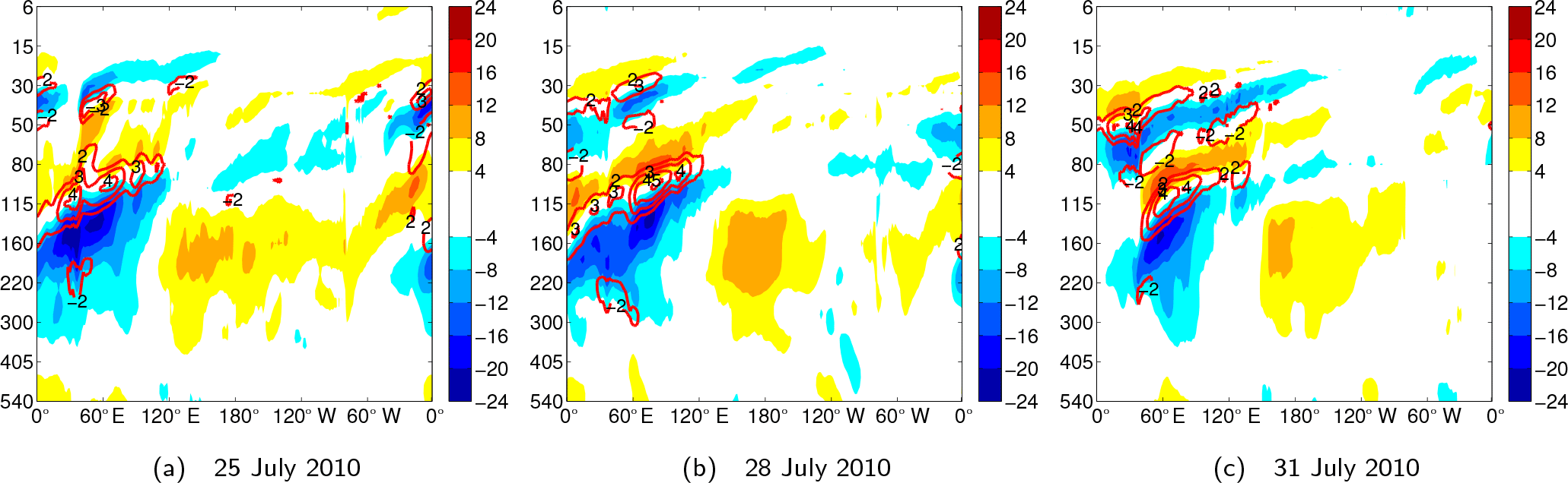
Figure 2Longitude–pressure cross section of the Kelvin wave (KW) zonal wind (red-blue shaded contours) and temperature (red contours) perturbations along 0.7^∘ N on (a) 25 July, (b) 28 July and (c) 31 July 2010. Temperature is shown every 1 K, starting at 2 K. Zonal winds are drawn every 4 m s⁻¹. Zero lines are omitted.

Download

Figure 2 illustrates day-to-day filtered KW fields along the equator on three separate July days in 2010, namely 25, 28 and 31. Both zonal wind (blue-to-red shades) and temperature fields (red contours) are shown. Without any predefined constrains on the KW propagation, one can observe a rich variety of KW behaviour occurring in time: from the quasi-stationary dipole patterns centred at 160 hPa to a wave package of free-propagating wave structures in the stratosphere transiting from the western into the eastern hemisphere.

In the stratosphere, the uppermost easterly wind component in blue shades around 30–50 hPa moves in eastward and downward directions, demonstrating the upward transport of KW energy (Andrews et al., 1987). KW amplitudes were largest over the eastern hemisphere with temperatures up to 4 K and zonal winds up to 12 m s⁻¹. The large amount of KW activity occurred during the easterly phase of the QBO with strong easterly winds present between 30 and 80 hPa (not shown), providing favourable conditions for strong KW activity.

Between 100 and 200 hPa during the second half of July, there was low-frequency KW activity present in the form of a stationary and robust “wave-1” pattern with strong KW easterly winds up to 24 m s⁻¹ in the eastern hemisphere and KW westerly winds up to 10 m s⁻¹ in the western hemisphere. The high vertical resolution within the TTL resolves shallow KW structures and a typical slanted structure towards the east in KW easterlies as well. The appearance and strength of horizontal KW response coincides with the presence of strong easterly winds in the TTL in the eastern hemisphere during this period (not shown). Figure 2 also shows that below 300 hPa the KW activity decreases and we shall not discuss levels under 300 hPa in this paper.

The zonal wind and temperature components are coupled through Eq. (3), which states that the amplitude of the negative KW temperature perturbation is proportional to the negative vertical gradient in geopotential (and vice versa), as well as in the zonal wind since the zonal wind and geopotential are in phase. Horizontally, the cold anomaly is always located between the westerly and the easterly phase of the zonal wind component. Vertically, maximal positive temperatures are observed between easterly winds below and westerly winds above. An estimate of the vertical wavelength can be made based on alternating zonal wind minima and maxima. For example, on 25 July a well-developed KW package extending into the stratosphere moved from the western into the eastern hemisphere. A quasi-stationary component of the wave package is observed around 60^∘ E with easterly winds located at 50 (∼21.5 km) and 150 hPa (∼13.5 km), implying a vertical wavelength of around 8 km.

More examples based on a daily basis filtered data from the 10-day deterministic forecast of the ECMWF can be found on the MODES website¹.

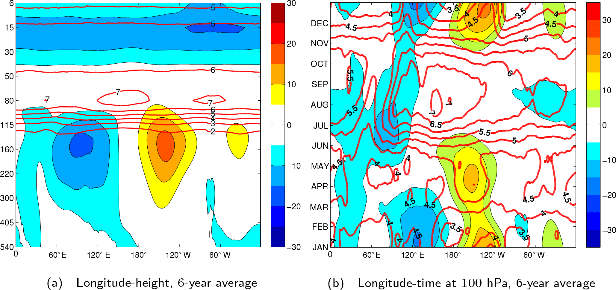
Figure 3Six-year average of the zonal wind and static stability fields of the ECMWF operational analyses. Both fields are latitudinally averaged over 5^∘ S–5^∘ N, and have been low-pass filtered a priori with a cut-off period of 90 days to highlight seasonal variability. (a) Longitude–height section and (b) longitude–time section at 100 hPa. Zonal winds are coloured by blue-to-red contours, each 5 m s⁻¹, whereas and static stability is shown in red contours, each (a) $\mathrm{1}\times {\mathrm{10}}^{-\mathrm{4}}$ s⁻² and (b) $\mathrm{0.5}\times {\mathrm{10}}^{-\mathrm{4}}$ s⁻². Zero lines are omitted.

Download

2.3 Other data and impact of the background state

In addition to the outputs from modal decomposition, full zonal wind and temperature fields from ECMWF analyses are used to compute the background fields based on the same N64 grid and over the same period (January 2007–June 2013). Zonal wind U and static stability N are latitudinally averaged in the belt 5^∘ S–5^∘ N on all model levels to produce their zonal structure.

Static stability profiles are estimated through

in units of s⁻² and are defined on hybrid model levels on which the geopotential field ϕ and the potential temperature field Θ are derived a priori from the input data. Both fields are shown in Fig. 3.

The zonal wind field has the largest values on average in the TTL around 150 hPa with westerly winds peaking in the western hemisphere over the Pacific Ocean and easterly winds peaking in the eastern hemisphere over the Indian Ocean and Indonesia. It represents a typical time-averaged outflow pattern in response to tropical convection (e.g. Fueglistaler et al., 2009). Throughout the seasons there is a longitudinal shift of this pattern following the convective source which is most clearly observed at 150 hPa. Such a seasonal shift is visible up to 100 hPa in Fig. 3b where winds are weaker compared to 150 hPa. In northern winter, zonal winds are strongest over Indonesia and the eastern Pacific with the zonal wind maxima position and strength similar compared to the longer ERA-40 dataset used by Suzuki and Shiotani (2008). During boreal summer, easterly winds mainly prevail over the Indian Ocean, which is linked to the Indian monsoon season.

At 100 hPa, the static stability illustrates the strongest seasonal cycle with values ranging from near-tropospheric values of $\mathrm{3}\times {\mathrm{10}}^{-\mathrm{4}}$ m s⁻² during northern winter towards stratospheric values of 5–6 $\times {\mathrm{10}}^{-\mathrm{4}}$ m s⁻² during boreal summer. Note also the resolved local maxima in static stability at 80 hPa above the warm pools, known as the tropical inversion layer (TIL) and which is possibly wave-driven (Grise et al., 2010; Kedzierski et al., 2016). Figure 3b suggests that the TIL descends down to 100 hPa during boreal summer months peaking over the western Pacific, in agreement with the cycle found in GPS-RO observations by Grise et al. (2010).

KWs are subject to wave modulation in changing background environments. Along its trajectory, the potential energy of the KW changes with varying background winds and stability which can be largely described by linear wave theory as long as waves are not near their critical level involving breaking and dissipation (Andrews et al., 1987). For simplification, KW modulation can be examined for the case of pure zonal as well as pure vertical wave propagation based on the wave modulation analysis performed by Ryu et al. (2008). A few key points on their local wave action conservation principle are summarized in the following.

In the tropical atmosphere, zonal modulation is the dominant process for KWs propagating in the stratosphere and in all non-easterly winds in the TTL. Vertical modulation becomes important in the presence of easterly winds within the TTL. Zonal modulation is found to affect both u_kw and T_kw components and their amplitudes are proportional to the Doppler-shifted phase speed by $(c-U{)}^{\mathrm{1}/\mathrm{2}}$ in the case of a pure zonal propagation direction. This means that KWs diminish in amplitude over regions with westerly winds and become more prone to dissipative processes, while amplify over regions with easterly winds². In the case of pure vertical modulation, the change in wave potential energy mainly fluctuates with the temperature component of the KW. Along the rays' vertical path, the waves amplitude is proportional to the Brunt–Väisälä frequency as $\propto N^{\mathrm{3}/\mathrm{2}}$, and to the Doppler-shifted phase speed as $\propto (c-U{)}^{-\mathrm{1}/\mathrm{2}}$, such that N is expected to play a primary role above 120 hPa where its value starts increasing rapidly (see Fig. 3).

Alexander and Ortland (2010) showed through wave modulation principles that temporal variations in zonal-mean N indeed are correlated with observed KW amplitudes at 16 km (approx. 100 hPa). A more extensive wave modulation analysis was described by Flannaghan and Fueglistaler (2013) using the full ray-tracing equations to demonstrate that zonal winds in the TTL not only modulate KWs locally but also create a lasting modulating effect on wave activity through ray convergence in the stratosphere. In particular, the seasonal cycle of the upper tropospheric easterlies (on average located over the western Pacific), that acts as an escape window for KWs throughout the year and largely explains the longitudinal structure of KW zonal wind and temperature climatology.

We shall present the seasonal variability in tropical convection by using the OLR dataset with daily outputs from the NOAA Interpolated OLR product (Liebmann and Smith, 1996). The OLR product, often used as a proxy for convection, is extracted on a $\mathrm{2.5}{}^{\circ }\times \mathrm{2.5}{}^{\circ }$ grid and interpolated on a N64 grid. Latitudinal averages are derived over a larger domain, namely over 15^∘ S–15^∘ N since organized convection tends to happen more remote from the equator, especially during the summer monsoon season over the Asian continent.

3.1 Energy distribution of KWs

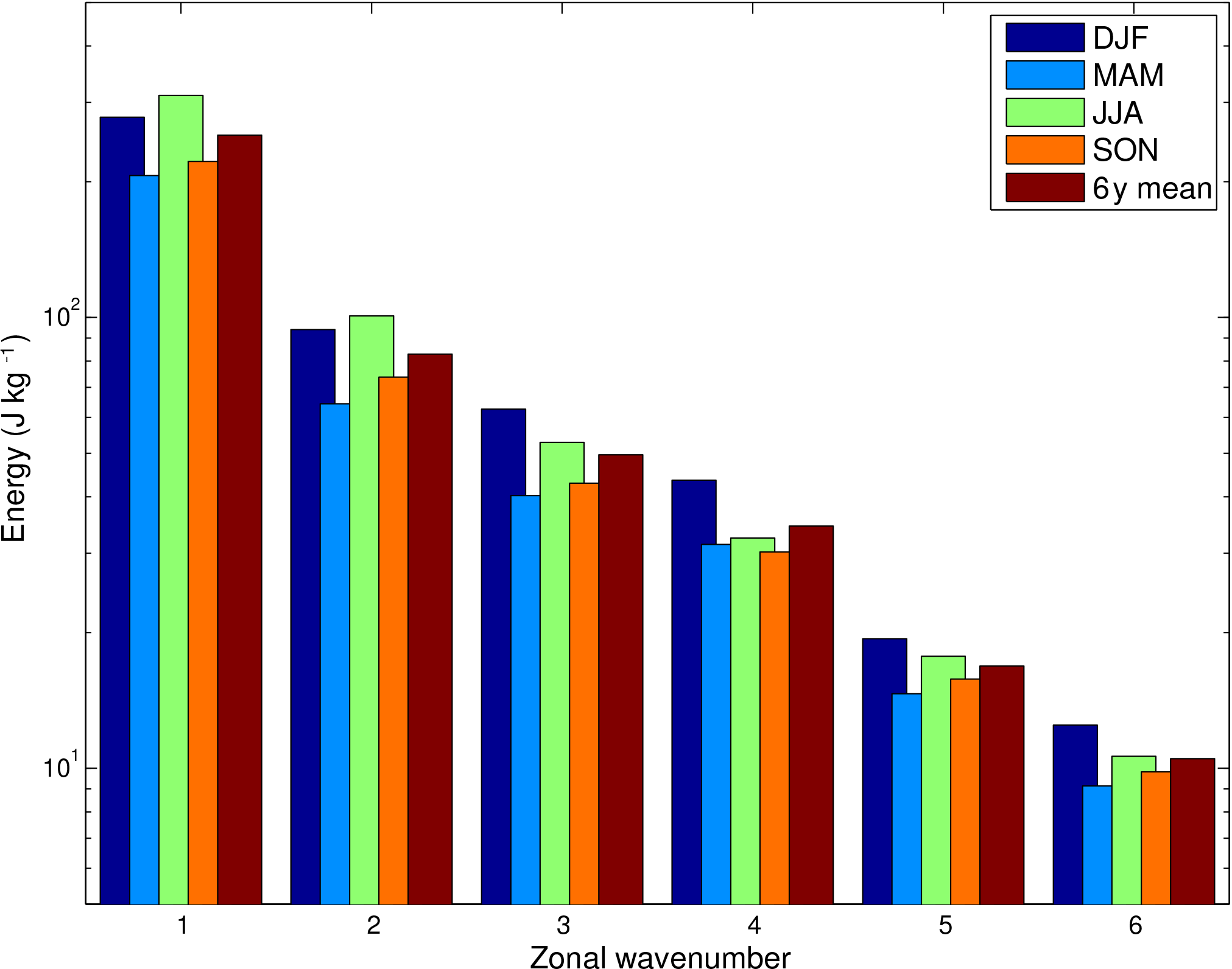
The seasonal cycle in the energy–zonal-wavenumber spectra is shown in Fig. 4 after summing up over all vertical modes. On average, energy decreases as the zonal wavenumber increases as typical for atmospheric energy spectra. As we deal with large scales, we show only the first 6 zonal wavenumbers with energy values shown separately for the annual mean and the four seasons separately.

Figure 4 shows that largest seasonal variations in KW energy are found at the largest zonal scales. For all zonal wavenumbers, above annual-mean energy values are observed during DJF and JJA seasons while SON and MAM are below annual-mean energy. In the zonal wavenumber 1, total KW energy varies between 200 J kg⁻¹ in MAM season and somewhat over 300 J kg⁻¹ in JJA. In wavenumber 2, values do not exceed 100 J kg⁻¹ and JJA still contains the largest energy. At higher wavenumbers, DJF season becomes the most energetic. In k>4, total KW energy is under 20 J kg⁻¹ and continue to reduce with k. The slope of the KW energy spectrum is between $-\mathrm{5}/\mathrm{3}$ and −1 at planetary scales (not shown), similar to the spectra presented in Žagar et al. (2009) for July 2007 data. The JJA spectra has on average the steepest slope compared to other seasons, in particular the DJF spectra. The energy distribution on planetary scales is mainly associated with large-scale tropical circulation established in response to ongoing tropical convection. Therefore, the zonal distribution of tropical convection may likely play a crucial role in explaining DJF and JJA season differences of KW energy, which will be explored in the next section.

Figure 4Kelvin wave (KW) energy (in J kg⁻¹) as a function of the zonal wavenumber k for k=1 to 6. For each k, seasonal averages are shown along with the total average as described by the legend. Energy is vertically integrated over 60 vertical modes. Further details are in Sect. 3.1.

Download

3.2 Seasonal cycle of KW energy

Figure 5 illustrates more details on the seasonal cycle by showing KW energy–time series at the largest scales represented by zonal wavenumbers k=1, k=2 and remaining scales k>2. During most JJA seasons and occasionally in DJF (e.g. 2008) the total amount of KW energy in k=1 can reach up to 600 J kg⁻¹, or twice the JJA average. The minimum in k=1 KW energy mainly occurs during October followed by April with values dropping towards 100 J kg⁻¹, or half the SON average. The temporal pattern in k=2 is similar to the k=1 pattern, but with a less pronounced semiannual cycle with maximum values up to 200 J kg⁻¹ and minimum values towards 30 J kg⁻¹. On zonal scales k>2, KWs still show a semiannual cycle with highest vertically integrated values of energy in DJF.

In particular, for zonal wavenumber k=1 one can distinguish inter-monthly in addition to semiannual variability. Inter-monthly variability is most clearly observed during JJA, for example in July 2011 where one can distinguish six separate peaks of over 400 J kg⁻¹ energy over a period of approximately 90 days resembling an average wave period of about 18 days. These are typical periods for free-propagating KWs as observed in the TTL and lower stratosphere (e.g. Randel and Wu, 2005). Note here again that our KW energy is vertically integrated over the whole model depth. This means that the observed inter-monthly variability in KWs appears to be dominated by the cyclic process of free-propagating KWs entering the TTL, amplifying due to changing environmental conditions, followed by wave breaking or dissipation.

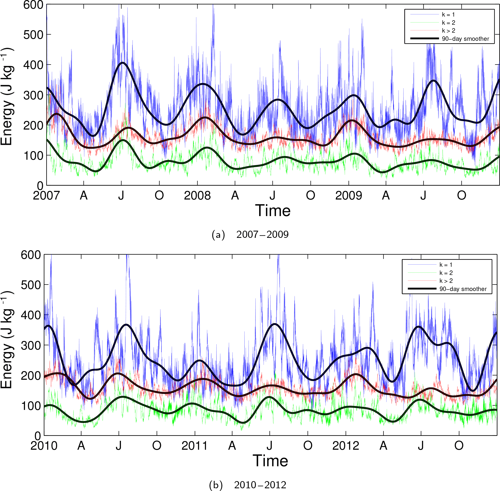
Figure 5Time series of the global total KW energy for various zonal wavenumbers over the following periods: (a) 2007–2009 and (b) 2010–2012. Labels on the x axis “A”, “J” and “O” refer to the first days of April, July and October, respectively. Presented are the zonal wavenumbers k=1 (blue line), k=2 (green line) and all smaller zonal scales, k>2 (red line). A 90 day low-pass filter has been applied (black lines) for each time series in order to filter out high-frequency variability and to highlight seasonal variability.

Download

The dominant scales of temporal variability in KWs are illustrated by a frequency spectrum of k=1 in Fig. 6. The spectrum is produced by the Fourier transform of energy time series of 6.5 years. The resulting power spectrum has been smoothed by taking the Gaussian-shaped moving averages over the raw spectrum by using the Daniell kernel three times (Shumway and Stoffer, 2010). The spectrum contains a peak at 1 day period associated with the diurnal tide partially projecting on the KWs. After that, a gradual increase in energy is seen towards the 16-day period with multiple individual periods standing out. For periods longer than 20 days, individual peaks are found close to 25, 43 and 59 days. After that, most KW energy is contained by far in the semiannual cycle. The frequency spectrum provides a useful starting point for the discussion in the next section when the spatiotemporal patterns of KWs shall be examined in several spectral domains.

Returning to Fig. 5, a low-pass filter with 90-day cut off has been applied on KW energy in order to keep only the two main spectral peaks in Fig. 6. The result is visible as the thicker black line in Fig. 5 for all three zonal wavenumber groups. A semiannual cycle for all zonal wavenumbers is evident with most energy observed around January and July, while least energy is observed approximately one month after the equinoxes. During the years 2007, 2010, 2011 and 2012, more k=1 KW energy is observed during JJA compared to the follow-up DJF season. The DJF of 2009–2010 was, for example, above average with energy values for k=1 above 350 J kg⁻¹.

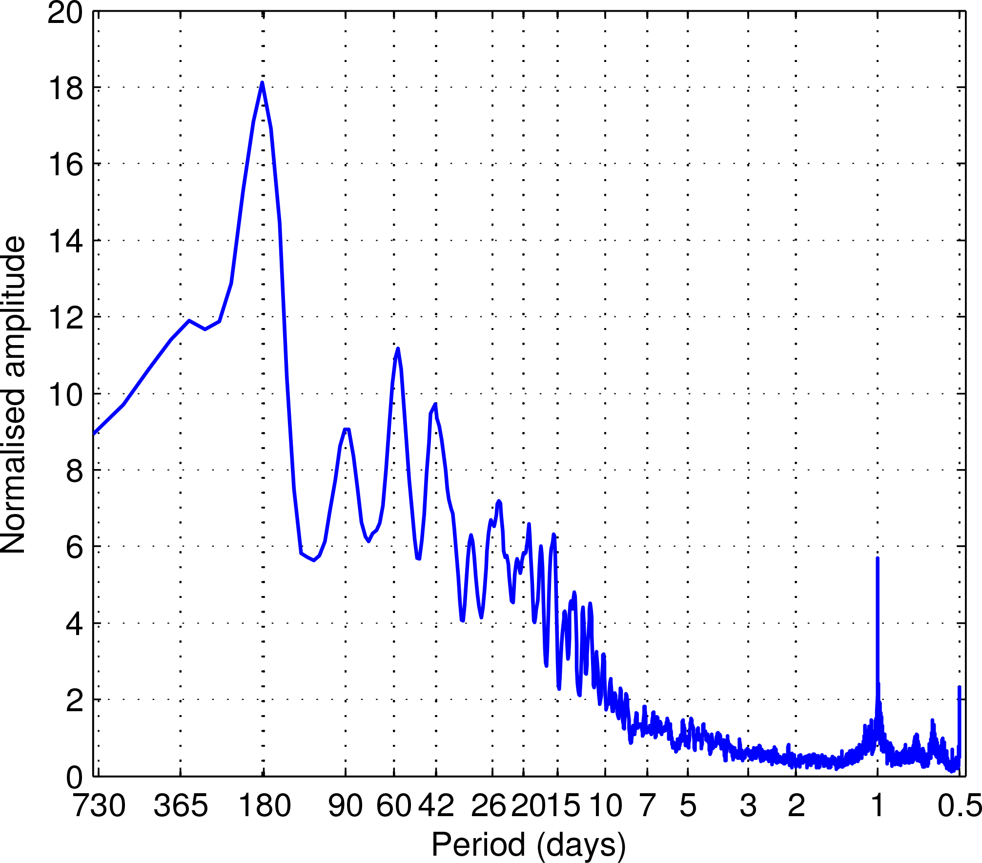
Figure 6Kelvin wave (KW) frequency spectrum for the zonal wavenumber k=1. The 1-2-1 filter with a Daniell kernel has been used to smooth the initial raw power spectra.

Download

The year-to-year differences can be explained by many coupled factors. In general, one expects the vertically integrated KW activity to increase when background wind conditions become favourable, i.e. in the presence of easterly winds. This occurs in the TTL in relation to strong convective outflow (Garcia and Salby, 1987; Suzuki and Shiotani, 2008; Ryu et al., 2008; Flannaghan and Fueglistaler, 2013) during DJF and JJA seasons mainly. Moreover, KW activity is enhanced whenever easterly QBO winds are present down into the lower stratosphere (Baldwin and Coauthors, 2001; Alexander and Ortland, 2010) or during El Niño (Yang and Hoskins, 2013). The latter factor may partly explain a large difference in the KW energy during the El Niño DJF of 2009–2010 and the below-average energy level a year after, during the strong La Niña DJF period of 2010–2011. However, during the La Niña DJF of 2007–2008, the amount of KW energy is above normal. That season, however, was characterized by above-normal Madden–Julian Oscillation activity which often occurs during favourable easterly QBO conditions in the stratosphere (Son et al., 2017). During 2010–2011, DJF season stratospheric winds were largely westerly thereby prohibiting KW activity. The role of these low-frequency atmospheric phenomena on KW seasonal variability is a topic of further research.

Finally, Fig. 5 also shows that KW activity in July 2007, previously examined by Žagar et al. (2009), was exceptionally strong. A large part of that energy, (somewhat more than half) belonged to zonal wavenumber 1. In spatiotemporal terms, it is associated with the presence of a strong dipole structure in the TTL (as in Fig. 2), which is colocated with favourable easterly wind conditions in the TTL as well as in the stratosphere (not shown). In fact, at 50 hPa the QBO was just at the beginning of its easterly phase in July 2007.

4.1 KW decomposition among wave periods

In this section, the spatiotemporal view of KWs shall be presented over three dominant ranges of wave periods in Fig. 6, namely (i) the (semi)annual cycle using a low-pass filter with cut-off period at 90 days, (ii) the intra-seasonal period using a bandpass filter over periods between 20 and 90 days and finally (iii) the intra-monthly period with bandpass filtered periods between 3 and 20 days. The chosen periods, especially the intra-monthly periods, are similar to those used in previous studies. In each case, mean 6-year fields as well as seasonal means shall be presented.

Note that our temporal filtering operates on time series of KW signals at every grid point. This is different from the commonly applied space-time filtering following Hayashi (1982) that applies KW dispersion relations. Our filtered KWs can appear stationary or even westward-shifted due to westward-moving sources of the KW amplification (e.g. easterly winds, high static stability in the TTL).

Both KW components u_kw and T_kw are Fourier-transformed to frequency space where the spectral expansion coefficients χ_kw in domains outside the desired frequency ranges are put to zero. Case (i) results in KW components u_kw,l and T_kw,l where l indicates the low-frequency component. Case (ii) results in u_kw,m and T_kw,m where m indicates the intra-monthly period. Case (iii) results in fields u_kw,h and T_kw,h where h stands for the high-frequency component. Previous studies have defined free-propagating KWs over similar ranges (3–20 days, Alexander and Ortland, 2010; 4–23 days, Suzuki and Shiotani, 2008) and similarly for intra-seasonal periods (23–92 days, Suzuki and Shiotani, 2008). Next, seasonal averages will be taken over the four seasons, resulting in variables ${\stackrel{\mathrm{‾}}{u_{\mathrm{kw},\mathrm{l}}}}^s$ and ${\stackrel{\mathrm{‾}}{T_{\mathrm{kw},\mathrm{l}}}}^s$ for the low-frequency component and similarly for the other two cases. The superscript s represents one of the four seasons: northern winter (s= DJF), spring (s= MAM), summer (s= JJA) and autumn (s= SON).

Cases (ii) and (iii) contain purely subseasonal variability and therefore one can expect their 6-year means to be zero-valued since variability beyond 90 days has been put to zero. Similarly, mean fields for each of the four seasons result in ${\stackrel{\mathrm{‾}}{u_{\mathrm{kw},\mathrm{h}}}}^s\ll {\stackrel{\mathrm{‾}}{u_{\mathrm{kw},\mathrm{l}}}}^s$ and ${\stackrel{\mathrm{‾}}{u_{\mathrm{kw},\mathrm{m}}}}^s\ll {\stackrel{\mathrm{‾}}{u_{\mathrm{kw},\mathrm{l}}}}^s$ and the same for the temperature component. This reflects the fact that positive and negative phases of the fast KW responses average out to approximately zero on seasonal timescales (figure not shown). Therefore, the seasonal mean of the absolute amplitudes of the zonal wind and temperature are examined instead, i.e. ${\stackrel{\mathrm{‾}}{\left|u_{\mathrm{kw},\mathrm{h}}\right|}}^s$ and ${\stackrel{\mathrm{‾}}{\left|u_{\mathrm{kw},\mathrm{m}}\right|}}^s$ and similarly for temperature. This describes seasonal fluctuations in subseasonal KW amplitudes³.

Figure 7Longitude–pressure sections along 0.7^∘ N of the KW zonal wind and temperature averaged over the 6-year period for (a) low-frequency, (b) intra-seasonal and (c) intra-monthly periods. The contouring is as follows: (a) zonal wind is coloured each 1.5 m s⁻¹ and temperature is shown by red contours each 0.5 K, with zero lines omitted; (b) absolute amplitudes of the zonal wind and temperature are shown in grey shades each 0.5 m s⁻¹ and red contours, each 0.15 K, respectively and (c) absolute amplitudes of the zonal wind are in grey shades each 0.25 m s⁻¹ and temperature in red contours (each 0.15 K).

Download

Figure 7 shows results for all three cases after taking means over the whole period. The left panel resembles a dominant “wave-1” structure with zonal wind maximized around 140 hPa. Easterly KW winds are strongest around 60^∘ E and westerly winds around the International Date Line. Note that two stationary perturbations over African (30^∘ E) and South American (80^∘ W) orography are the result of our terrain-following NMF analysis. If one compares the KW zonal wind pattern with the climatological zonal wind pattern in Fig. 3a, it can be observed that the zonal wind pattern is located around 20^∘ west of the climatological pattern. Wave temperature perturbations are largest where the vertical gradients in zonal wind are largest, which explains the quadrupole structure. Warm and cold KW anomalies are located at 100 hPa in the eastern and western hemispheres, respectively, and vice versa at 200–300 hPa.

The average low-frequency or seasonal KW structure has a significant resemblance with the classical Gill-type KW solution (Gill, 1980) describing a steady-state linear wave response to convective forcing. The Gill-type KW solution is characterized by westerly upper-troposphere winds east of the large-scale convective source. In response to the seasonal cycle of convection, the solution in Fig. 7a also illustrates, in addition to a low-frequency KW variability in westerly winds, a considerable low-frequency variability west of the convective outflow. This part of the signal represents the wave modulation effect of the propagating KWs on seasonal timescales.

The middle panel of Fig. 7 shows the average distribution of KW activity on intra-seasonal timescales. The activity is largest in the eastern hemisphere with average zonal wind maxima up to 3 m s⁻¹ and temperature maxima up to 0.7 K. Zonal wind activity is largest over a broad area between 90 and 150 hPa over the Indian Ocean and the Maritime Continent. Temperature activity occurs slightly higher around 90–100 hPa. Intra-seasonal activity is locally somewhat increased also around 120^∘ W, west of the Andes mountain range.

Finally, Fig. 7c illustrates the average distribution of intra-monthly KWs. The eastern hemisphere again makes up for the larger KW activity than the western hemisphere, but the maximum is located more upward in comparison to the intra-seasonal scales, around 80 hPa. Zonal wind activity peaks up to 3 m s⁻¹ over a broad range of 70–110 hPa and temperature peaks over a more narrow area around 76 hPa (up to 0.75 K). The main area for KW activity is found over the Indian Ocean region, while least wave activity is above the central Pacific. Towards the stratosphere, KW activity reduces and becomes more uniform along the longitudinal direction.

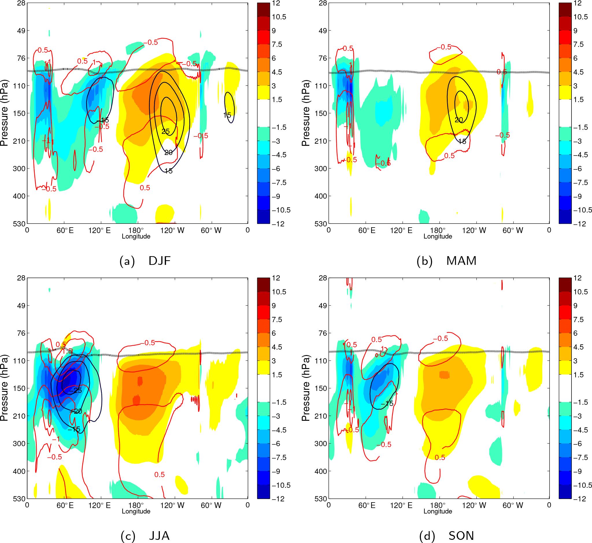
Figure 8Seasonally averaged longitude–pressure sections of the KW zonal wind (blue-to-red colour-filled contours) and temperature (red contours) along 0.7^∘ N. (a) DJF, (b) MAM, (c) JJA and (d) SON. Contouring of the KW signal is the same as in Fig. 7a. A single static stability contour with value $\mathrm{5}\times {\mathrm{10}}^{-\mathrm{4}}$ s⁻² is shown as a thick dotted black line to represent the seasonal movement of the tropical tropopause height. The average background zonal wind is shown by blue contours (each 5 m s⁻¹, starting from 15 m s⁻¹). The background zonal wind and stability fields are latitudinally averaged over 5^∘ S–5^∘ N. All fields are smoothed using a low-pass filter with the cut-off period of 90 days.

Download

4.2 Low-frequency KW variability

The seasonal patterns of the low-frequency components of the KW is presented as pressure–longitudinal cross sections along the equator (at 0.7^∘ N) of the KW seasonal means, given by ${\stackrel{\mathrm{‾}}{\left[u_{\mathrm{kw},\mathrm{l}}\right]}}^s$ and ${\stackrel{\mathrm{‾}}{\left[T_{\mathrm{kw},\mathrm{l}}\right]}}^s$ in Fig. 8.

The largest amplitudes are found during the JJA months. A strong dipole “wave-1” pattern is evident in the TTL. The strongest zonal winds are found close to 150 hPa with easterlies up to −12 m s⁻¹ centred over the Indian Ocean and westerlies up to 6 m s⁻¹ over the western Pacific. Negative temperature KW anomalies at 110 hPa are strongest as well during JJA with values up to 1.5 K over the Indian Ocean and annually averaged value of −0.5 K over the western Pacific.

During DJF, the dipole pattern has shifted more eastward and upward compared to JJA and has a more slanted structure. Easterly (westerly) KW winds are located more east over the Maritime continent (central Pacific) and are centred at 130 hPa. The upper temperature dipole pattern is found higher up at approximately 90 hPa. Values are somewhat weaker compared to Northern Hemisphere summer with easterlies up to −6 m s⁻¹ and westerlies up to 5 m s⁻¹.

Finally, SON and MAM season months are transition seasons with respect to the strength and position of the KW dipole as it moves west- and downward towards JJA and east- and upward towards DJF. Season MAM has the weakest KW dipole with slightly stronger westerly winds up to 5 m s⁻¹.

The longitudinal position and the strength of the low-frequency KWs have been linked to the seasonal patterns of the background winds in the TTL representing the upper level monsoon and Walker circulations (Flannaghan and Fueglistaler, 2013). The average background winds maximize at 150 hPa as shown in Fig. 3a. In Fig. 8, one can see how the KW easterlies in the eastern hemisphere are strongest during JJA in relation to the Indian and South Asian monsoon circulation. Background easterlies as strong as −30 m s⁻¹ are located approximately 10^∘ east of the KW maximum easterlies. Season DJF has the strongest background westerlies in relation to the upper-level circulation of the western Pacific anticyclones. Season MAM shows similar background wind patterns compared to DJF but with weaker circulation. Season SON shows similar patterns with JJA but with weaker winds.

Further details on longitudinal position and interannual variability in the low-frequency KW response at its maximum value at 150 hPa are illustrated by the Hovmöller diagram in Fig. 9. For comparison, tropical convection is represented as well through the OLR proxy variable averaged over 15^∘ S–15^∘ N latitudes. All fields have been filtered with a 90-day cut-off low-pass filter in order to highlight the seasonality. As a result, one can observe enhanced or reduced KW activity during the same individual seasons as seen from the time series in Fig. 5. Above-average seasonal KW activity with stronger dipole structures occurred during the summer of 2007 (mainly through its easterlies at 60^∘ E) and during the winters of 2006–2007 and 2009–2010. In these winters, El Niño was active and a clear longitudinal eastward shift is observed in OLR and in the background circulation (not shown), as well as in the dipole KW structure. The El Niño winter of 2009–2010 was followed by a strong La Niña winter with an increase in tropical convection over the Maritime Continent (note OLR values below 195 Wm⁻²).

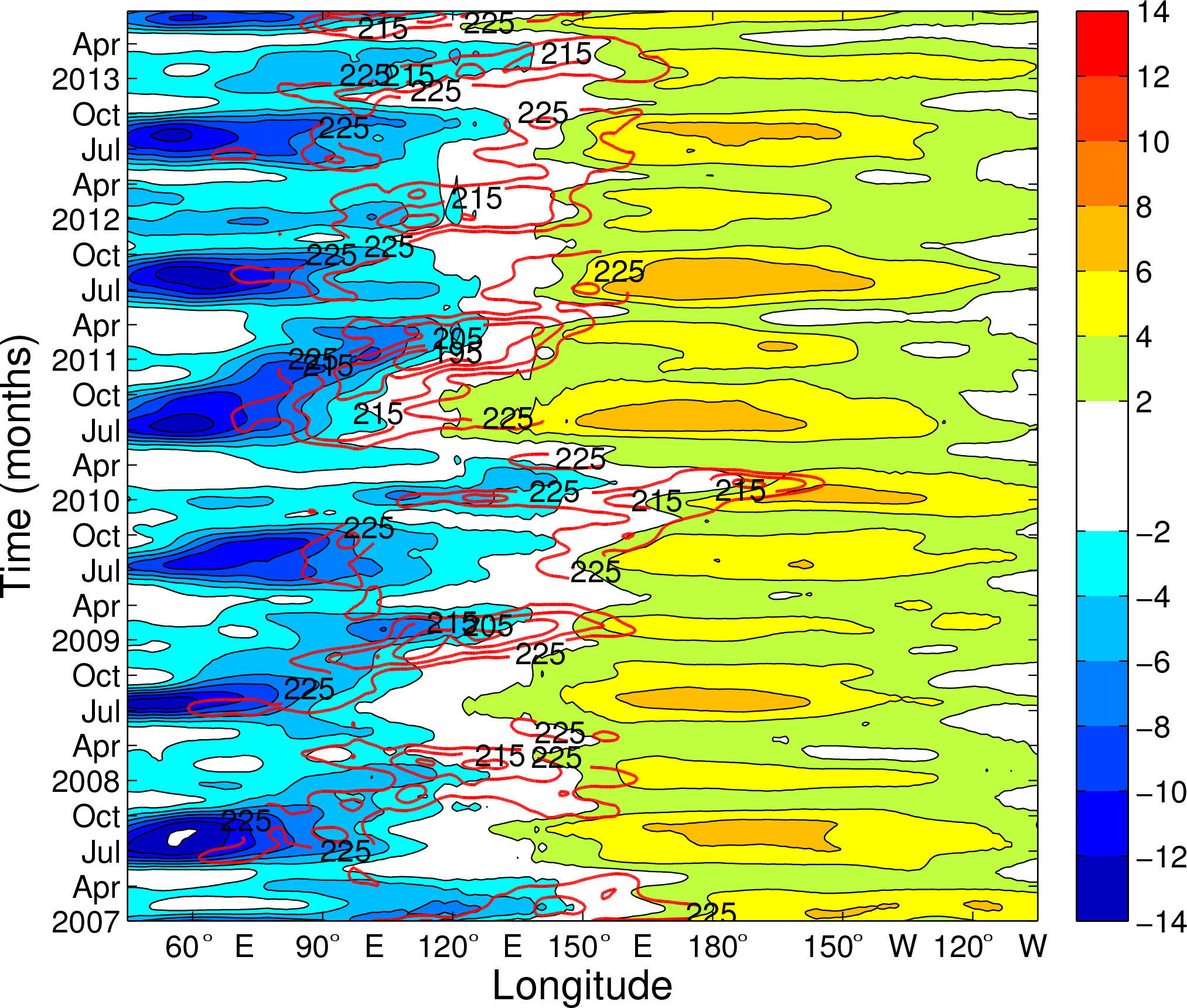
Figure 9Longitude–time section at model level 45 (∼153 hPa) of the KW zonal wind along 0.7^∘ N (blue to red shaded contours every 2 m s⁻¹ with zero line omitted) and the outgoing longwave radiation (OLR) averaged over the latitude belt 15^∘ S–15^∘ N (red contours each 10 Wm⁻² starting at 225 Wm⁻²). Both fields have been filtered a priori using a low-pass filter with a cut-off period of 90 days.

Download

The vertical seasonal movement of the KW dipole has been linked with the seasonal movement of the tropical tropopause height (Flannaghan and Fueglistaler, 2013; Ryu et al., 2008). The position of the tropical tropopause height (represented by a static stability value of $\mathrm{5}\times {\mathrm{10}}^{-\mathrm{4}}$ s⁻² in Fig. 8) is found at approximately 85 hPa during DJF and descends towards 100 hPa in JJA, similar to values obtained from GPS-RO observations by Grise et al. (2010). In particular, during JJA, one can notice how the asymmetry in the tropical tropopause height over the Indian Ocean around 60^∘ E coincides with increasing temperatures by the KW dipole up to 1.5 K. Such deformation of the tropical tropopause is also evident during DJF and SON seasons.

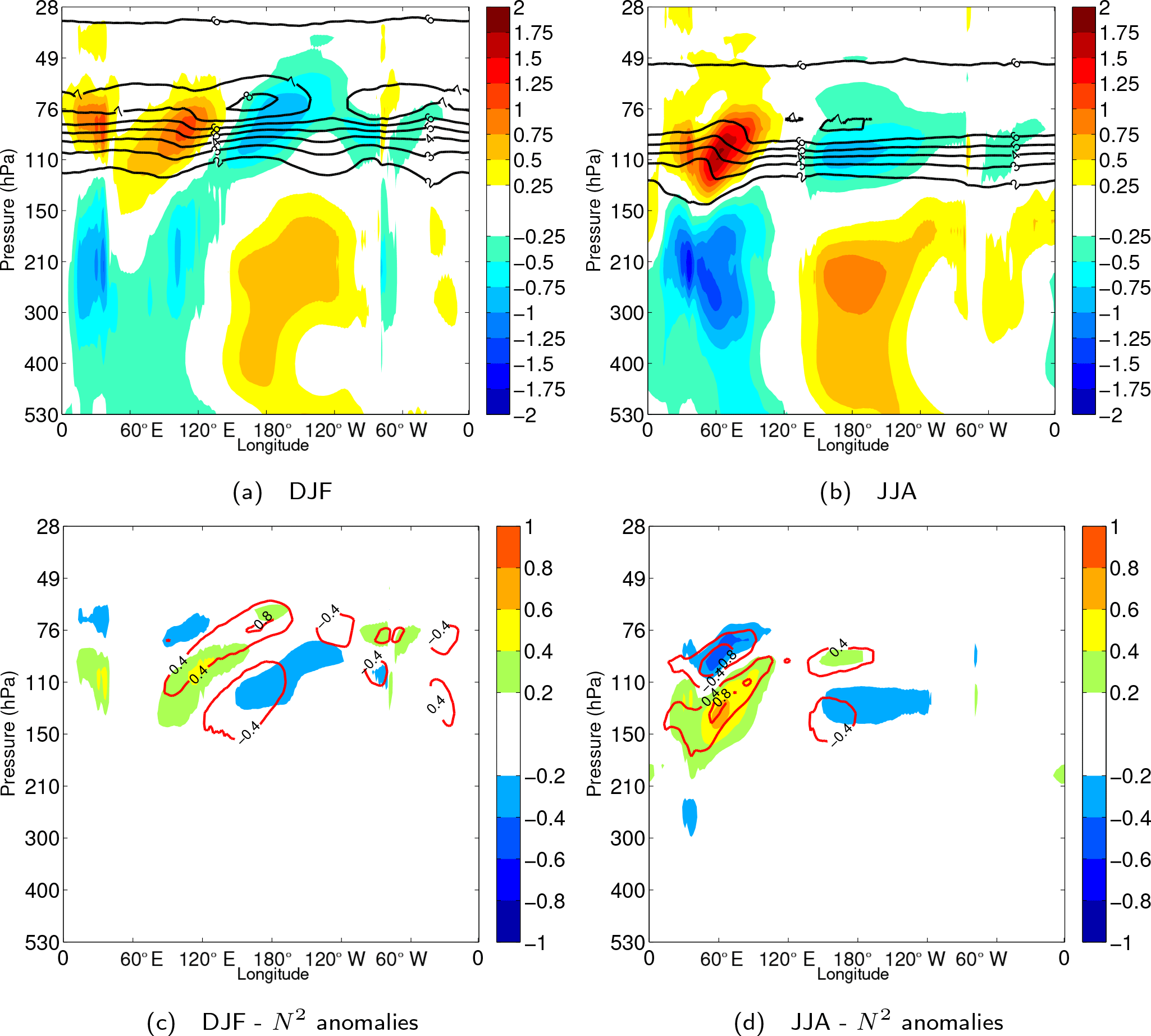
Figure 10Seasonally averaged longitude–pressure sections for (a, c) DJF and (b, d) JJA. (a–b) KW temperature, ${\stackrel{\mathrm{‾}}{T_{\mathrm{kw}}}}^s$, (blue-to-red shades every 0.25 K) and static stability field, ${\stackrel{\mathrm{‾}}{N^{\mathrm{2}}}}^s$ (black contours, each $\mathrm{1}\times {\mathrm{10}}^{-\mathrm{4}}$ s⁻², starting at $\mathrm{2}\times {\mathrm{10}}^{-\mathrm{4}}$ s⁻²). (c–d) KW static stability anomaly, ${\stackrel{\mathrm{‾}}{N_{\mathrm{kw}}^{\mathrm{2}}}}^s$ (blue-to-red, each $\mathrm{0.2}\times {\mathrm{10}}^{-\mathrm{4}}$ s⁻²), and static stability anomaly with respect to the zonal mean, ${\stackrel{\mathrm{‾}}{{N^{\prime }}^{\mathrm{2}}}}^s$ (red contours, each $\mathrm{0.4}\times {\mathrm{10}}^{-\mathrm{4}}$ s⁻²).

Download

Figure 10a and b illustrate seasonal-mean KW temperatures ${\stackrel{\mathrm{‾}}{T_{\mathrm{kw},\mathrm{l}}}}^s$ in relation to the tropical tropopause layer defined by static stability N². Seasonal variations in KW temperatures are colocated with the position of the tropopause, descending down from its highest position during DJF to its lowest position during JJA. Temperature amplitudes are observed to decline roughly above $N^{\mathrm{2}}=\mathrm{5}-\mathrm{6}\times {\mathrm{10}}^{-\mathrm{4}}$ s⁻². Within this zonal-mean seasonal picture, zonal asymmetries in N² exist and are found: (i) near the International Date Line with values of $\mathrm{8}\times {\mathrm{10}}^{-\mathrm{4}}$ s⁻² at 80 hPa during DJF and $\mathrm{7}\times {\mathrm{10}}^{-\mathrm{4}}$ s⁻² at 90 hPa during JJA and (ii) lower at 100 hPa over the Indian Ocean during JJA. Particularly during JJA, the deformation of the zonal-mean static stability field colocates strongly with the position of a strong KW temperature anomaly over the Indian Ocean. A rough estimation is made on the contribution of the KW anomaly to the zonal deformation of the tropopause layer by removing zonal-mean parts of both fields. First, static stability zonal anomalies, ${\stackrel{\mathrm{‾}}{{N^{\prime }}^{\mathrm{2}}}}^s$, are derived by subtracting zonal-mean values of N² from the full N² field per time step and at every pressure level, followed by seasonal averaging. Next, we can estimate the static stability change associated with the KW anomaly, using the relation $N_{\mathrm{kw}}^{\mathrm{2}}=\frac{g}{\stackrel{\mathrm{‾}}{\mathit{\theta }}}\frac{\partial {\mathit{\theta }}_{\mathrm{kw}}}{\partial z}$, followed by seasonal averaging as well, i.e. ${\stackrel{\mathrm{‾}}{N_{\mathrm{kw}}^{\mathrm{2}}}}^s$.

As a result, Fig. 10c and d show how both static stability anomalies are overlapping. During DJF, the structure of the zonal anomaly ${\stackrel{\mathrm{‾}}{{N^{\prime }}^{\mathrm{2}}}}^s$ has a positively valued tilt eastward which stretches up to 80 hPa, while during JJA a strong static stability anomaly is found more localized over the Indian Ocean region with values in the TTL up to ${\stackrel{\mathrm{‾}}{{N^{\prime }}^{\mathrm{2}}}}^{\mathrm{JJA}}=\pm \mathrm{0.8}\times {\mathrm{10}}^{-\mathrm{4}}$ s⁻². The anomaly associated with the KW temperature is found to peak up to $+\mathrm{0.6}\times {\mathrm{10}}^{-\mathrm{4}}$ s⁻² during JJA and up to $+\mathrm{0.4}\times {\mathrm{10}}^{-\mathrm{4}}$ s⁻² during DJF. Finally, by dividing both fields with each other, the resulting contribution of the quasi-stationary KW to the observed deformation of the tropical tropopause layer is estimated up to 60 % during JJA and 80 % during DJF.

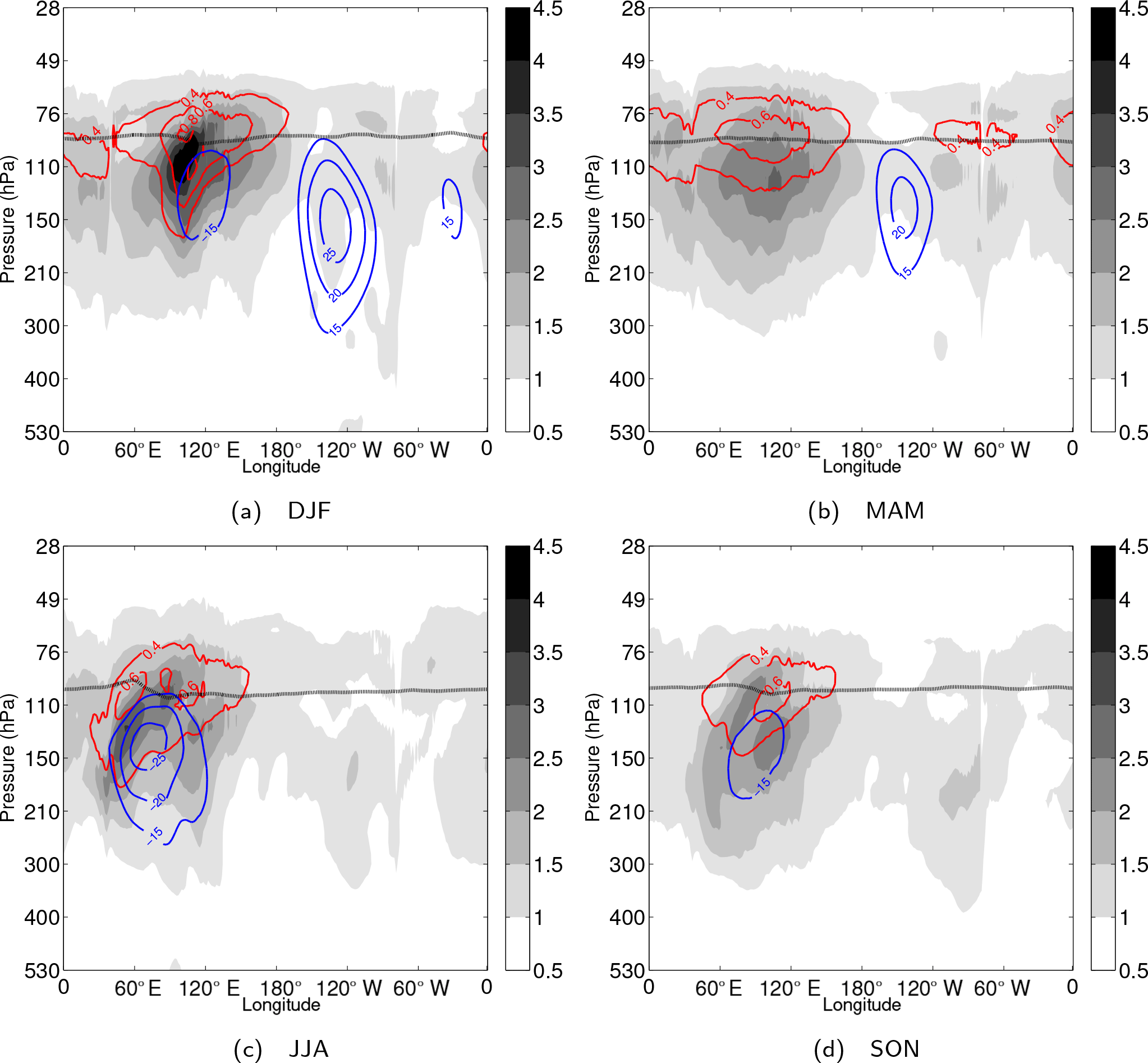
Figure 11Seasonally averaged longitude–pressure sections along 0.7^∘ N of the intra-seasonal KW zonal wind (white-to-black shades, each 0.5 m s⁻¹) and temperature (red contours, each 0.2 K). (a) DJF, (b) MAM, (c) JJA and (d) SON. The averaging is performed for the absolute values of both zonal wind and temperature perturbations. The background zonal wind (shown by blue contours) and the tropical tropopause height (single thick dotted contour) are defined as in Fig. 8.

Download

4.3 Intra-seasonal KW variability

The seasonality of intra-seasonal KW variability is shown in Fig. 11 and shall be briefly discussed here. The DJF stands out as the most active season for KW activity, located mainly in the eastern hemisphere centred at 100^∘ E and with maximum activity at 110 hPa for zonal wind and temperature with a second maximum in temperature at 90 hPa. Values observed are up to 0.8 K for KW temperature and 5 m s⁻¹ for KW zonal wind. During the MAM season, the KW activity fields are weaker but spread over a larger area in the eastern hemisphere and in the TTL with maximum activity centred at 120 hPa (90 hPa) for the zonal wind (temperature) component. Both JJA and SON seasons have KW activity positioned at lower altitudes and more westward. In both seasons, KW zonal wind activity is split up between two structures with an eastward tilt with height: one with a maximum around 110^∘ E and one pattern starting from 100 hPa and extending towards 60^∘ E. Note also the increase in KW activity in the western hemisphere below 150 hPa in the east Pacific. The maximum KW activity in the temperature component for both seasons is positioned near 100 hPa approximately on the tropical tropopause contour with a value $\mathrm{5}\times {\mathrm{10}}^{-\mathrm{4}}$ s⁻².

The eastward tilted structure is observed throughout all seasons except MAM when background easterly winds are nearly absent in the eastern hemisphere. In all other seasons one can observe how the tilted structure is locked to the background easterlies with maximum amplitudes located slightly above and west of it. Such eastward tilt with height has been frequently observed, for example over a radiosonde station Medan at 100^∘ E during the early stage of Madden–Julian Oscillation development (Kiladis et al., 2005).

Figure 12As in Fig. 11 but for the intra-monthly KWs. The zonal wind (white-to-black shades) is drawn every 0.25 m s⁻¹.

Download

4.4 Intra-monthly KWs

The seasonal variability in intra-monthly KWs, represented by their absolute amplitudes ${\stackrel{\mathrm{‾}}{\left|u_{\mathrm{kw},\mathrm{h}}^{\prime }\right|}}^s$ and ${\stackrel{\mathrm{‾}}{\left|T_{\mathrm{kw},\mathrm{h}}^{\prime }\right|}}^s$, shall be examined in relation to the background conditions. Figure 12 illustrates favourable regions for KW activity. In general, KW activity increases upward from around 120 hPa towards its zonal-mean peak value at 76 hPa. The largest values are observed in the eastern hemisphere in a region from 30 to 150^∘ E. The temperature component in particular has a constant maximum peak (up to 0.8 K) located around 76 hPa throughout the year, where the largest increase in N² also occurs as shown in Fig. 3. Above 70 hPa, KW activity continuously decreases in the stratosphere.

The longitudinal structure of the KW zonal wind shows two distinct peaks in the TTL, one consistently located at 76 hPa and another around 100–110 hPa in the eastern hemisphere, which is mainly present during solstice seasons. The first maximum coincides with the temperature distribution, which can be explained by their balance relationships and free horizontal propagation in the stratosphere. Below the tropopause, KW activity is coupled to convective processes alternating the tropospheric vertical wave structures as discussed by Flannaghan and Fueglistaler (2012).

The secondary maximum around 110 hPa in Fig. 12 is present mainly during solstice seasons in the eastern hemisphere and it is associated with the seasonal movement of the background wind.

The maximum of KW wind and the background wind maximum move eastward from DJF to JJA seasons similar to the low-frequency variability.

A day-by-day comparison of the KW activity and background wind confirms that propagating KWs amplify while approaching a region of strong easterlies, forming a folding structure around it while the individual KWs dissipate towards the centre of easterly winds. In Fig. 12 one can notice a fast reduction of KW amplitudes eastward of its maximum towards the centre of the background easterlies. It is likely related to dissipation and wave breaking processes as observed over Indonesia (120^∘ E) by Fujiwara et al. (2003). Within such regions, the KW–background-wind interaction becomes complex and the linearity assumption breaks (Ryu et al., 2008; Flannaghan and Fueglistaler, 2013).

A comparison with the previous study by Suzuki and Shiotani (2008) using ERA-40 data shows that the L91 data contain stronger KW activity in the vicinity of the background easterlies in the eastern hemisphere, and more fine-scale details, which can be explained by better analyses based on more observations and improved models including increased resolution. For example, Suzuki and Shiotani (2008) used 5 levels of ERA-40 data between 50 and 200 hPa whereas the present study considers 25 model levels between 50–200 hPa. Maxima of the KW temperature signal appear in similar locations and strength, except for a small offset in vertical position (70 hPa in Suzuki and Shiotani, 2008, versus 80 hPa in Fig. 12) and a larger zonal asymmetry in our results.

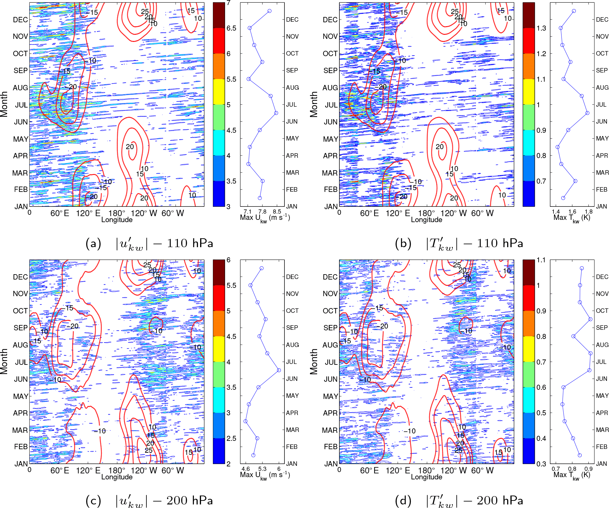
Figure 13Intra-monthly KW zonal wind and temperature composites as a function of longitude and month in a calendar year at (a–b) model level 40 (∼110 hPa) and (c–d) model level 49 (∼200 hPa) along 0.7^∘ N. The waves are accumulated from different years into a single calendar year to highlight seasonal behaviour. Only the most energetic signals are shown: (a, c) zonal wind, $\left|u_{\mathrm{kw}}^{\prime }\right|$, each 0.5 m s⁻¹, and (b, d) temperature $\left|T_{\mathrm{kw}}^{\prime }\right|$, each 0.1 K. For comparison, the background zonal wind field is presented by red contours, each 5 m s⁻¹. On the right side of each panel, blue lines with circles denote maximal amplitude of the KW zonal wind occurring anywhere along the equator averaged over the 6-year period for each calendar month. This highlights seasonality in the maximum amplification of propagating KWs.

Download

Another view of the seasonal cycle of free-propagating KWs is illustrated in Fig. 13, which focuses on the spatiotemporal distribution of individual KW tracks. Hovmöller diagrams are illustrated for KW zonal wind and temperature at levels 110 and 200 hPa cumulated from different years into a single calendar year along with the background zonal wind. In addition, the monthly-mean values of daily maximum KW amplitudes occurring in longitude are added on the right side of each diagram. It represents seasonality in the KW maximum amplitudes in a similar fashion to Fig. 6 in Alexander and Ortland (2010), which is based on HIRDLS satellite data.

The individual wave tracks at 110 hPa illustrate KWs with amplitudes exceeding 3 m s⁻¹ and 0.6 K, which are propagating throughout the year in the eastern hemisphere, during June–October months only over the Pacific, and all except DJF months in most of the western hemisphere. Typical wave tracks start east of the 0^∘ (30^∘ W) meridian during winter (summer) and largely disappear west of 120^∘ E. The largest wave amplitudes are observed between 50 and 100^∘ E prior to regions of easterly winds in agreement with Fig. 12. Here, presented details show that the most notable waves appear during the Asian monsoon period with upper-level easterlies prevailing from June into September. The largest KW amplitudes appear to be confined to the June and July months followed by a rapid drop in August. In fact, a local minimum in the number of KWs as well as in wave amplitudes occurs in August before the KW activity increases slightly during autumn.

At 200 hPa, the favourable area for KW propagation shifts to the western hemisphere and high KW activity is observed west of the South American continent throughout the year (west of 80^∘ W) with a westward extension over the Pacific during JJA. Another set of wave tracks starts over equatorial South America around 30^∘ W and continues until 60^∘ E during JJA. During DJF these wave tracks shift more east and start at 5^∘ W and continue until 90^∘ E. The seasonal shifts of approximately 30^∘ in KW tracks colocate with similar shifts in the prevailing TTL winds.

The amplitude of KWs undergoes a clear annual cycle with a small secondary peak present during DJF, as represented by the monthly-means of daily maximum amplitudes on the right side of Fig. 13. The largest amplitudes are found at 110 hPa during JJA with monthly-mean zonal wind (temperature) values up to 8.5 m s⁻¹ (1.8 K) in June. During the DJF months KWs amplify more eastward with monthly-mean zonal wind (temperature) values up to 7.8 m s⁻¹ (1.6 K) in December. Our result matches well with the observed seasonal pattern in maximum KW temperatures at 16 km (∼ 100 hPa) from the HIRDLS satellite observations (Alexander and Ortland, 2010, Fig. 6). At 200 hPa, KW amplitudes are on average lower with a yearly-averaged amplitude reduction around 55 % in temperature and 35 % in zonal wind.

The semiannual cycle in maximum amplitudes remains visible up until 70 hPa. Above 70 hPa, where the KW activity remains large in the eastern hemisphere (Fig. 12), the semiannual cycle is replaced by an interannual cycle in line with the dominant impact of the QBO.