the Creative Commons Attribution 4.0 License.
the Creative Commons Attribution 4.0 License.
 | 13 Jun 2018
Assessing the capability of different satellite observing configurations to resolve the distribution of methane emissions at kilometer scales
Alexander J. Turner
Daniel J. Jacob
Joshua Benmergui
Jeremy Brandman
Laurent White
Cynthia A. Randles
Anthropogenic methane emissions originate from a large number of fine-scale and often transient point sources. Satellite observations of atmospheric methane columns are an attractive approach for monitoring these emissions but have limitations from instrument precision, pixel resolution, and measurement frequency. Dense observations will soon be available in both low-Earth and geostationary orbits, but the extent to which they can provide fine-scale information on methane sources has yet to be explored. Here we present an observation system simulation experiment (OSSE) to assess the capabilities of different satellite observing system configurations. We conduct a 1-week WRF-STILT simulation to generate methane column footprints at 1.3 × 1.3 km2 spatial resolution and hourly temporal resolution over a 290 × 235 km2 domain in the Barnett Shale, a major oil and gas field in Texas with a large number of point sources. We sub-sample these footprints to match the observing characteristics of the recently launched TROPOMI instrument (7 × 7 km2 pixels, 11 ppb precision, daily frequency), the planned GeoCARB instrument (2.7 × 3.0 km2 pixels, 4 ppb precision, nominal twice-daily frequency), and other proposed observing configurations. The information content of the various observing systems is evaluated using the Fisher information matrix and its eigenvalues. We find that a week of TROPOMI observations should provide information on temporally invariant emissions at ∼ 30 km spatial resolution. GeoCARB should provide information available on temporally invariant emissions ∼ 2–7 km spatial resolution depending on sampling frequency (hourly to daily). Improvements to the instrument precision yield greater increases in information content than improved sampling frequency. A precision better than 6 ppb is critical for GeoCARB to achieve fine resolution of emissions. Transient emissions would be missed with either TROPOMI or GeoCARB. An aspirational high-resolution geostationary instrument with 1.3 × 1.3 km2 pixel resolution, hourly return time, and 1 ppb precision would effectively constrain the temporally invariant emissions in the Barnett Shale at the kilometer scale and provide some information on hourly variability of sources.


Methane is a greenhouse gas emitted by a range of natural and anthropogenic sources (Kirschke et al., 2013; Saunois et al., 2016; Turner et al., 2017). Anthropogenic methane emissions are difficult to quantify because they tend to originate from a large number of potentially transient point sources such as livestock operations, oil or gas leaks, landfills, and coal mine ventilation. Atmospheric methane observations from surface and aircraft have been used to quantify emissions (e.g., Miller et al., 2013; Caulton et al., 2014; Karion et al., 2013, 2015; Lavoie et al., 2015; Conley et al., 2016; Peischl et al., 2015, 2016; Houweling et al., 2016) but are limited in spatial and temporal coverage. Satellite measurements have dense and continuous coverage but limitations from observational errors and pixel resolution need to be understood. Here we perform an observing system simulation experiment (OSSE) to investigate the information content of different configurations of satellite instruments for observing fine-scale and transient methane sources, taking as a test case the oil and gas production sector.
Low-Earth orbit satellite observations of methane by solar backscatter in the shortwave infrared (SWIR) have been available since 2003 from the SCIAMACHY instrument (2003–2012; Frankenberg et al., 2005) and from the GOSAT instrument (2009–present; Kuze et al., 2009, 2016). SWIR instruments measure the atmospheric column of methane with near-unit sensitivity throughout the troposphere. SCIAMACHY and GOSAT demonstrated the capability for high-precision (<1 %) measurements of methane from space (Buchwitz et al., 2015), but SCIAMACHY had coarse pixels (30 × 60 km2 in nadir) and GOSAT has sparse coverage (10 km diameter pixels separated by 250 km). Inverse analyses have used observations from these satellite-based instruments to estimate methane emissions at ∼ 100–1000 km spatial resolution (e.g., Bergamaschi et al., 2009, 2013; Fraser et al., 2013; Monteil et al., 2013; Wecht et al., 2014a; Cressot et al., 2014; Kort et al., 2014; Turner et al., 2015, 2016a; Alexe et al., 2015; Tan et al., 2016; Buchwitz et al., 2017; Sheng et al., 2018a, b). But such coarse resolution makes it difficult to resolve individual source types because of spatial overlap (Maasakkers et al., 2016).
Improved observations of methane from space are expected in the near future (Jacob et al., 2016). The TROPOMI instrument (Veefkind et al., 2012; Butz et al., 2012; Hu et al., 2016, 2018), launched in October 2017, will provide global mapping at 7 × 7 km2 nadir resolution once per day. The GeoCARB geostationary instrument (Polonsky et al., 2014; O'Brien et al., 2016) will be launched in the early 2020s with current design values of 3 × 3 km2 pixel resolution and twice-daily return time. Additional instruments are presently in the proposal stage with improved combinations of pixel resolution, return time, and instrument precision (Fishman et al., 2012; Butz et al., 2015; Xi et al., 2015).
An OSSE simulates the atmosphere as it would be observed by an instrument with a given observing configuration and error specification. Several OSSEs have been conducted to evaluate the potential of satellite observations to quantify methane sources, but they have been conducted at either coarse (∼ 50 × 50 km2) spatial resolution (Wecht et al., 2014b; Bousserez et al., 2016) or assumed idealized flow conditions (Bovensmann et al., 2010; Rayner et al., 2014). Here we use a 1-week simulation of atmospheric methane with 1.3 × 1.3 km2 resolution over a 290 × 235 km2 domain to simulate continuous and transient emissions in the Barnett Shale region of Texas, and from there we quantify the capability of different satellite instrument configurations to resolve and quantify these sources at the kilometer and hourly scales. Our choice of scales is guided by the resolution of the planned satellite observations, and our choice of the Barnett Shale is guided by the availability of a high-resolution emission inventory for the region (Lyon et al., 2015). The pattern and density of methane emissions in the Barnett Shale is typical of other source regions in the US (Maasakkers et al., 2016).
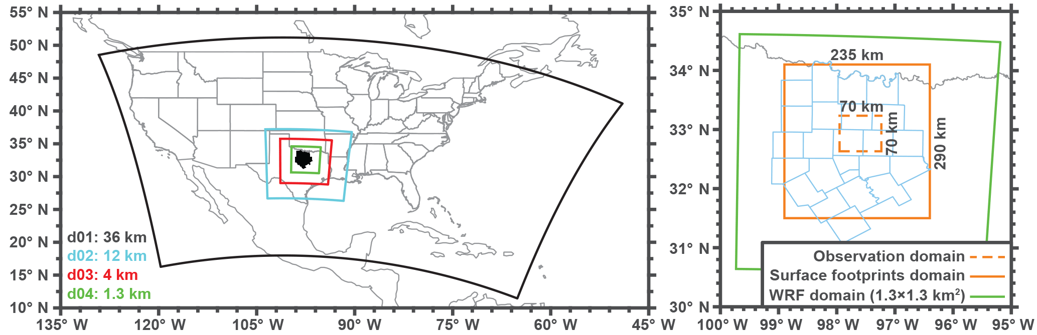
Figure 1High-resolution OSSE domain. Left panel shows the successive nested WRF domains at 36, 12, 4, and 1.3 km spatial resolutions, with the coarser domains providing initial and boundary conditions for the finer domains. Black shaded region is the Barnett Shale region in Texas. Right panel shows the domain for the OSSE. Green box is the innermost 1.3 km WRF domain, dashed orange box is the observation domain, and solid orange box is the domain over which the footprints are computed. Light blue lines indicate the counties in the Barnett Shale.
We simulate atmospheric methane concentrations over the Barnett Shale in Texas at 1.3 × 1.3 km2 horizontal resolution for the period of 19–25 October 2013 using a framework similar to that of Turner et al. (2016b). The simulation uses version 3.5 of the Weather Research and Forecasting (WRF) model (Skamarock et al., 2008) over a succession of nested domains (left panel in Fig. 1) with 1.3 × 1.3 km2 spatial resolution in the innermost domain covering 290 × 235 km2. There are 50 vertical layers up to 100 hPa. Boundary-layer physics are represented with the Mellor–Yamada–Janjíc scheme and the land surface is represented with the five-layer slab model (Skamarock et al., 2008). The simulation is initialized with assimilated meteorological observations from the North American Regional Reanalysis (https://www.ncdc.noaa.gov/data-access/model-data/model-datasets/north-american-regional-reanalysis-narr, last access: 4 May 2018). Overlapping 30 h forecasts were initialized every 24 h at 00:00 UTC and the first 6 h of each forecast were discarded to allow for model spinup. Grid nudging was used in the outermost domain.
WRF meteorology is used to drive the Stochastic Time-Inverted Lagrangian Transport (STILT) model (Lin et al., 2003). STILT is a Lagrangian particle dispersion model. It advects an ensemble of particles backward in time from selected receptor locations, using the archived hourly WRF wind fields and boundary-layer heights. STILT calculates the footprint for the receptors; a spatiotemporal map of the sensitivity of observations to emissions contributing to the concentration at each selected receptor location and time. We use STILT to calculate 10-day footprints for hourly column concentrations at 1.3 × 1.3 km2 resolution over a 70 × 70 km2 domain in the innermost WRF nest, tracking the resulting footprints over a 290 × 235 km2 domain (right panel in Fig. 1). With this system we examine the constraints on emissions over the 290 × 235 km2 domain provided by dense SWIR satellite observations (over the 70 × 70 km2 domain) that have up to 1.3 km pixel resolution and hourly daytime frequency. Footprints for each column are obtained by releasing 100 STILT particles from vertical levels centered at 28, 97, 190, and 300 m above the surface and 8 additional levels up to 14 km altitude spaced evenly on a pressure grid. The column footprints are then constructed by summing the pressure-weighted contributions from individual levels, using a typical SWIR averaging kernel taken from Worden et al. (2015) with near-uniformity in the troposphere and correcting for water vapor (see Appendix A in O'Dell et al., 2012).
The footprint for the ith receptor location and time can be expressed as a vector describing the sensitivity of the column concentration y at that receptor location and time to the emission fluxes x over the 290 × 235 km2 domain and previous times extending up to 10 days. Here x is arranged as a vector of length n assembling all the emission grid cells and hours, allowing the emissions to vary on an hourly basis. The column concentration is expressed as the dry air column-average mixing ratio (ppb) following common practice (Jacob et al., 2016). The emissions x have units of nmol m−2 s−1, so that the footprint has units of ppb nmol−1 m2 s. The column concentration for the ith observation (yi) can be reconstructed from its footprint as
where bi is the background column concentration upwind of the 290 × 235 km2 domain. We can then write the full set of observations as a vector y of length m and reshape the set of m footprint vectors h into an m×n sparse matrix (where m is the number of observations and n is the number of state vector elements):
where b is the background vector with elements bi and H is the Jacobian matrix that maps emissions to concentration enhancements due to emissions within our domain.
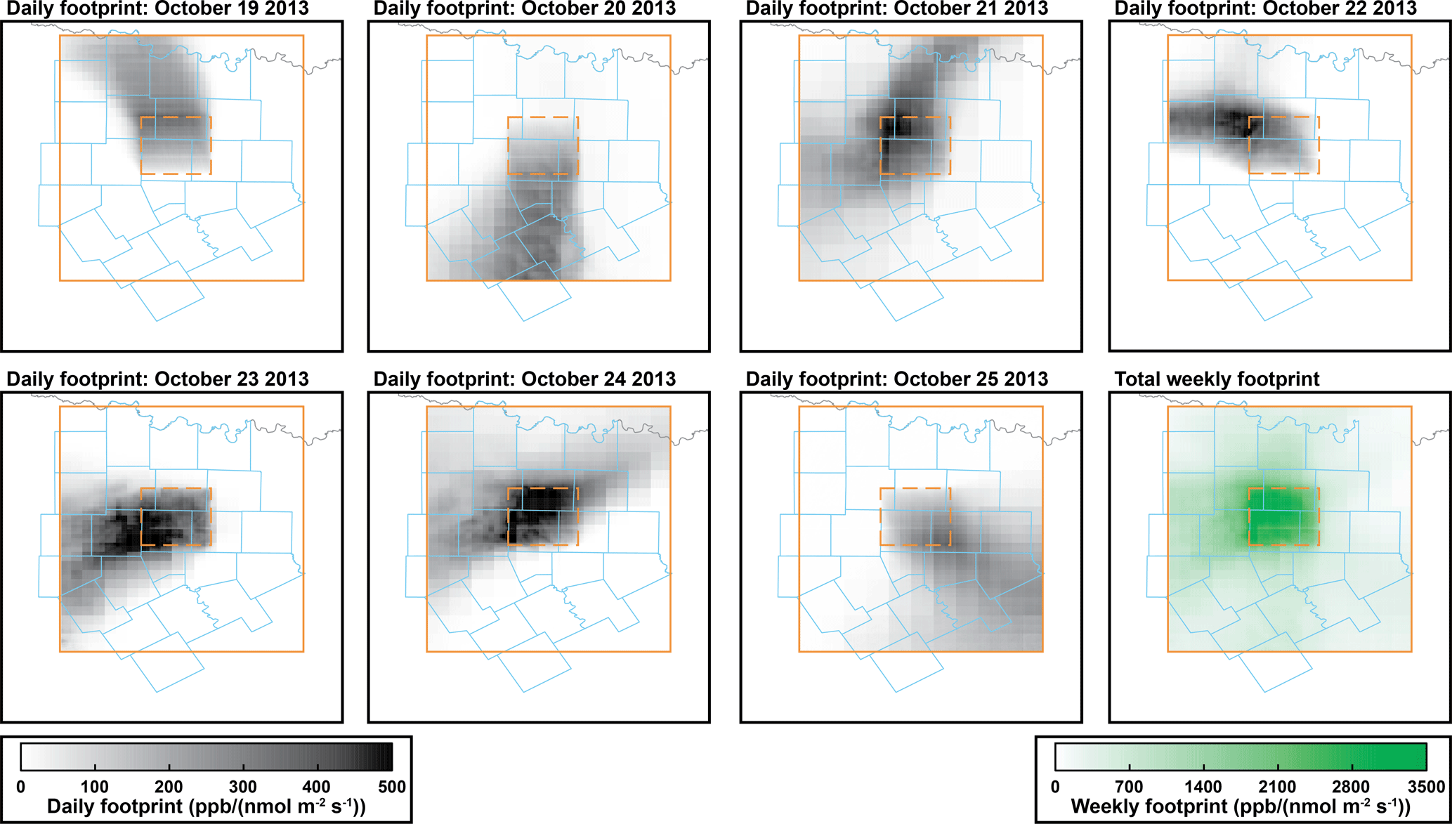
Figure 2Summed methane column footprints for all 1.3 × 1.3 km2 grid cells in the 70 × 70 km2 observation domain defined by the dashed orange box. The footprints are calculated from 08:00 to 17:00 LT over the 290 × 235 km2 domain defined by the solid orange box. Bottom right panel shows the summed footprint for the full week.
Figure 2 shows the sum of all column footprints produced on individual days for the 70 × 70 km2 observation domain. Computing these high-resolution footprints was a non-trivial computational task and ultimately yielded more than 4 Tb of footprints for the week of pseudo-satellite observations in the Barnett Shale. The footprints show large variability from day to day over the course of the week, reflecting meteorological variability. For example, winds are from the north on 19 October and from the south on 20 October. The winds are weak on 24 October, resulting in a strong local contribution to the footprint. Summing the footprints over the course of the week (bottom right panel of Fig. 2), we find that the observations are mainly sensitive to the core 70 × 70 km2 domain where they are made, with a diffuse sensitivity over the outer 290 × 235 km2 domain. Additional observations within the outer domain would need to be considered to constrain emissions in that domain. However, information on emissions in the 70 × 70 km2 core domain is mainly contributed by observations within the domain. Thus our focus will be to determine the capability of the observations in the 70 × 70 km2 domain to constrain emissions within that same domain, but we include the outer 290 × 235 km2 domain in our footprint analysis for completeness in accounting of information. Previous work Turner et al. (2016b, Supplement Sect. 6.1) investigated the impact of domain size on error reduction for WRF-STILT inversions in California's Bay Area and found that it had a negligible impact
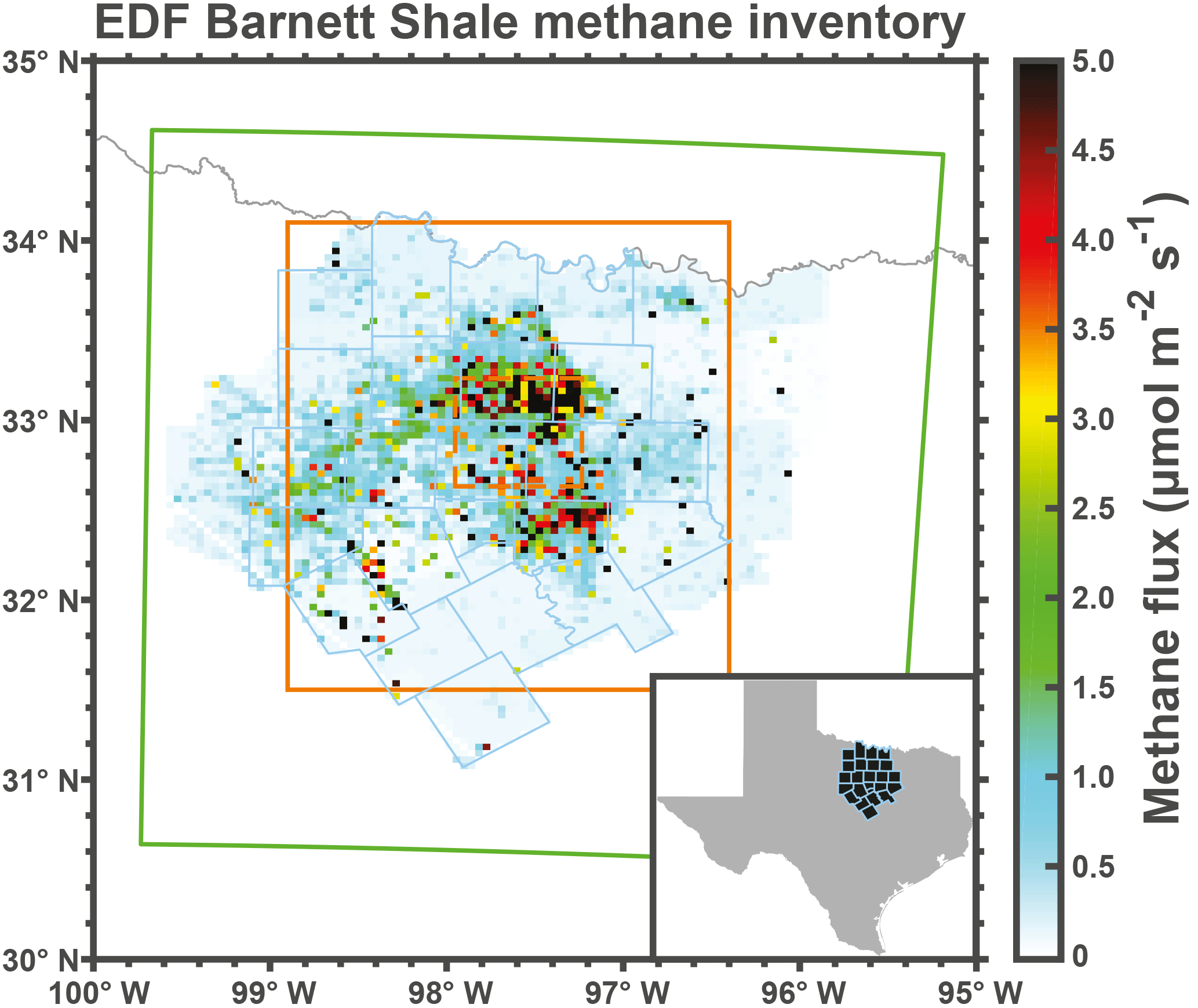
Figure 3Gridded Environmental Defense Fund (EDF) methane emission inventory for the Barnett Shale in Texas in October 2013 (Lyon et al., 2015). Spatial resolution is 4 × 4 km2. White areas are outside the inventory domain.
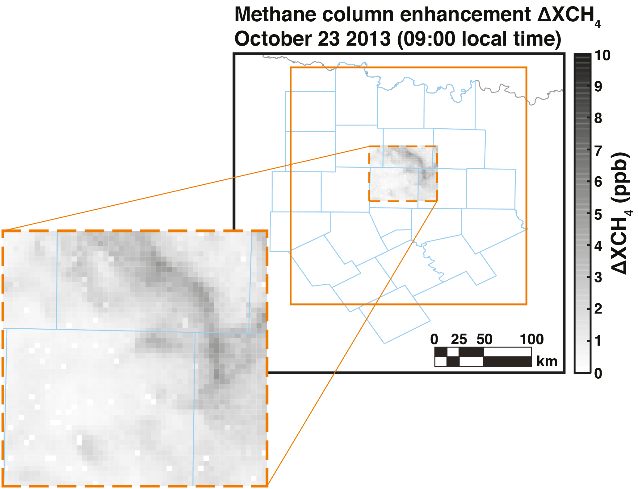
Figure 4Simulated methane concentration enhancements relative to background (ΔXCH4=Hx) in the 70 × 70 km2 observation domain of the Barnett Shale (dashed orange box), as derived from the downscaled EDF methane inventory (x) and the WRF-STILT footprints (H) within the 290 × 235 km2 OSSE domain (solid orange box). Values are for 23 October at 09:00 LT. Zeros are due to missing data because of unfinished computations.
The footprint information can be combined with an emission inventory for the 290 × 235 km2 domain to generate a field of column concentrations over the 70 × 70 km2 domain as would be observed from satellite. For this purpose we use the Environmental Defense Fund (EDF) inventory for the Barnett Shale in October 2013 at 4 × 4 km2 resolution compiled by Lyon et al. (2015). We downscale the EDF inventory by uniform attribution from 4 × 4 km2 to 1.3 × 1.3 km2 spatial resolution. The inventory is shown in Fig. 3 and includes contributions from oil and gas production, livestock operations, landfills, and urban emissions from the Dallas–Fort Worth area. It provides mean monthly values with no temporal resolution, but presumes that some sources will behave as sporadic large transients (Zavala-Araiza et al., 2015). Figure 4 shows an example of the methane column enhancements above background (Hx) computed at 09:00 local time on 23 October. We find enhancements in the range of 0–10 ppb due to emissions within the 290 × 235 km2 OSSE footprint domain. In what follows we will examine the potential of different satellite observing systems to detect these enhancements relative to the background and interpret them in terms of local sources.
Table 1Satellite observing systems considered in this work.
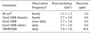
a Hourly observations are 10
times per day at 08:00–17:00 LT,
twice-daily observations are at 10:00 and 14:00 LT, and daily observations are at 13:00 LT.
b Aspirational instrument with the highest observation
frequency and pixel resolution that can be simulated within our OSSE
framework.
We aim to determine the information content from different satellite-based observing systems regarding the spatial and temporal distribution of emissions in the Barnett Shale. We consider both steady and potentially transient emissions with five different satellite observing configurations (Table 1). TROPOMI (global daily mapping, 7 × 7 km2 nadir pixel resolution, 11 ppb precision; Veefkind et al., 2012) was launched in October 2017 and is expected to provide an operational data stream by the end of 2018. GeoCARB (geostationary, 2.7 × 3.0 km2 pixel resolution, 4 ppb precision; O'Brien et al., 2016) is planned for launch in the early 2020s and its observation schedule is still under discussion with a tentative design for observations twice daily; here we examine different return frequencies of hourly, twice daily, and daily. Finally, the hypothetical “hi-res” configuration assumes geostationary hourly observations at the 1.3 × 1.3 km2 pixel resolution of our WRF simulation and with 1 ppb precision; it represents an aspirational system that combines the frequent return time, fine pixel resolution, and high precision of instruments presently at the proposal stage (Bovensmann et al., 2010; Fishman et al., 2012; Xi et al., 2015). All configurations are filtered for cloudy scenes.
The various satellite observing configurations of Table 1 differ in their return frequency, pixel resolution, and instrument precision. The benefit of improving any of these attributes may be limited by error in the forward model used in the inverse analysis (i.e., the Jacobian matrix H) and by spatial or temporal correlation of the errors. These limitations are described by the model–data mismatch error covariance matrix (R) including summed contributions from the instrument, forward model, and representation errors (Turner and Jacob, 2015; Brasseur and Jacob, 2017). Representation errors are negligible here because the instrument pixels are commensurate or coarser than the model grid resolution. Instrument error (i.e., precision) is listed in Table 1. Forward model error is estimated by computing STILT footprints for a subset of the meteorological period using the Global Data Assimilation System (GDAS; https://www.ncdc.noaa.gov/data-access/model-data/model-datasets/global-data-assimilation-system-gdas, last access: 4 May 2018) applying the two sets of footprints to either the EDF methane inventory (Fig. 3; Lyon et al., 2015) or the gridded EPA inventory (Maasakkers et al., 2016), and computing semivariograms of differences in column concentrations. From this we obtain a forward model error standard deviation of 4 ppb with an error correlation length scale of 40 km. We assume a temporal model error correlation length of 2 h. Sheng et al. (2018b) previously derived a temporal model error correlation length of 5 h in simulation of TCCON methane column observations at 25 km resolution, and we expect our correlation length to be shorter because of the finer resolution.
Bayesian inference is commonly used when estimating methane emissions with atmospheric observations, allowing for errors in the observations and in the prior estimates:
where P(x|y) is the posterior probability density function (pdf) of the state vector (x) given the observations (y), P(y|x) is the conditional pdf of y given x, and P(x) is the prior pdf of x. A common assumption is that P(y|x) and P(x) are normally distributed which allows us to write the posterior pdf as
where B is the n×n prior error covariance matrix and xa is the n×1 vector of prior fluxes. The most probable solution is obtained by minimizing the cost function:
yielding the posterior estimate ():
with an n×n posterior error covariance matrix:
that characterizes the uncertainty in the solution. The first term in the posterior covariance matrix is known as the Fisher information matrix: (see, for example, Rodgers, 2000; Tarantola, 2004).
Comparison between 𝓕 and B−1 identifies the extent to which the observations reduce the uncertainty in the fluxes. Specifically, the number of pieces of information on emissions acquired to better than measurement error is the number of eigenvalues of that are greater than unity (Rodgers, 2000). As such, the Fisher information matrix and prior error covariance matrix can quantify the effective rank of the observing system.
A drawback with this formulation of the information content is that it relies on the assumption of a Gaussian prior pdf. A number of papers have suggested that the pdf of methane emissions from a given source may be skewed, with a “fat tail” of transient high emissions (e.g., Brandt et al., 2014; Zavala-Araiza et al., 2015; Frankenberg et al., 2016). Alternate formulations for the cost function to be minimized may include no prior information (least-squares regression), a prior constraint that promotes a sparse solution (e.g., Candes and Wakin, 2008), a prior constraint based on frequentist regularization approaches (such as LASSO regression or Tikhonov regularization), or a prior constraint based on the spatial patterns of emissions rather than their magnitudes (geostatistical inversion). Table 2 lists the corresponding formulations. From Table 2 we see that the observation term is the same in all cases. Thus the Fisher information matrix provides a general measure of the information content provided by an observing system, independent of the form of the prior constraint, and we use it in what follows as a measure of the information content.
Table 2Cost functions for different formulations of the inverse problema.
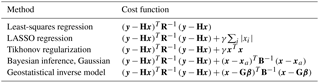
a γ is the regularization parameter for LASSO regression and Tikhonov regularization. G is a matrix with columns corresponding to different spatial datasets and β is a vector of drift coefficients for the spatial datasets. Other variables defined in the text.
The Fisher information matrix is an n×n matrix. Each of its n eigenvectors represent an independent normalized emission flux pattern and the corresponding eigenvalues are the inverses of the error variances associated with that pattern. A more useful way of stating this is that the inverse square root of the ith eigenvalue of 𝓕 represents the flux threshold fi needed for the observations to be able to constrain the emission flux pattern represented by the ith eigenvector. Whether that flux threshold is useful depends on the magnitude of the emissions, and this can be assessed for the problem at hand. Thus the eigenanalysis of the Fisher information matrix gives us a general estimate of the capability of an observing system to quantify emissions, which can then be applied to any actual n×n emission field.
For a given emission field, we may expect that some of the n emission flux patterns will be usefully constrained by the observing system while others are not. The number of patterns that are usefully constrained represents the number ℐ≤n pieces of information on emissions provided by the observing system. We will equivalently refer to it as the rank of the Fisher information matrix. This is determined by comparing the eigenvalues of an emission inventory (ei) to the flux thresholds. The number of ei larger than the corresponding fi provides a cut-off to estimate ℐ:
In the case of Bayesian inference, this is roughly equivalent to the degrees of freedom for signal with a diagonal prior error covariance matrix and a relative uncertainty of 100 %. But the eigenanalysis of the Fisher information matrix provides a more general approach of the capability of an observing system that can be confronted to any prior constraint and allows intercomparison of different observing system configurations.
There is an inconsistency in this formulation of ℐ: 𝓕 and B−1 have different eigenspaces. In this work we have chosen to treat these matrices separately because, in practice, it is computationally infeasible to directly compute the eigenvalues of the matrix product if n is large, as in the case here of constraining hourly emissions of the spatially distributed inventory. This inconsistency results in our estimate of ℐ likely being an upper bound on the information content (see Appendix for details).
The eigenanalysis of Sect. 3 allows us to intercompare the value of different satellite configurations for resolving the fine-scale patterns of methane emissions within a given domain. Here we apply it to the Barnett Shale domain of Sect. 2. We consider two limiting cases: Case 1 assumes the emissions to be temporally invariant and Case 2 assumes the emissions to vary hourly with no temporal correlation. In Case 1 the problem is typically overdetermined (m>n), depending on the satellite configuration, and the maximum rank of 𝓕 is n (the number of emission grid cells). In Case 2 the problem is underdetermined (m<n) and the maximum rank of 𝓕 is m (the number of observations).
In both Case 1 and 2, the observations only provide useful information (as defined by Eq. 8) if the signal is larger than the noise, as diagnosed by the ei>fi criterion of Eq. 8. Here the emissions are the downscaled EDF inventory, which includes 40 140 grid cells in the 290 × 235 km2 inversion domain (n= 40 140 in Case 1 with temporally invariant emissions) but only 2 601 of those grid cells are within the 70 × 70 km2 observation domain (dashed orange box in Fig. 1), where we might expect the observations to provide the strongest constraints. In Case 2 with temporally variable emissions we have grid cells for a single day.
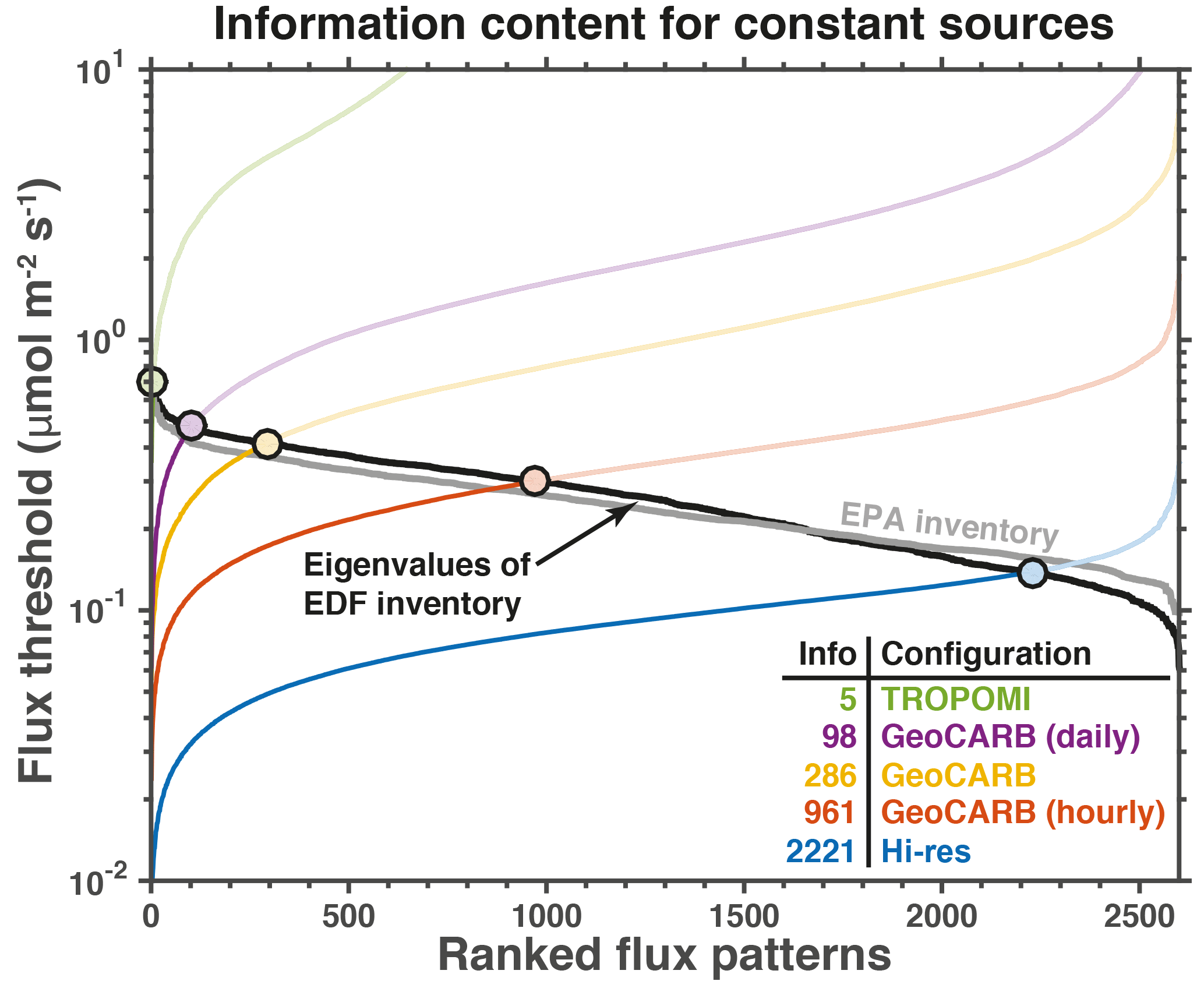
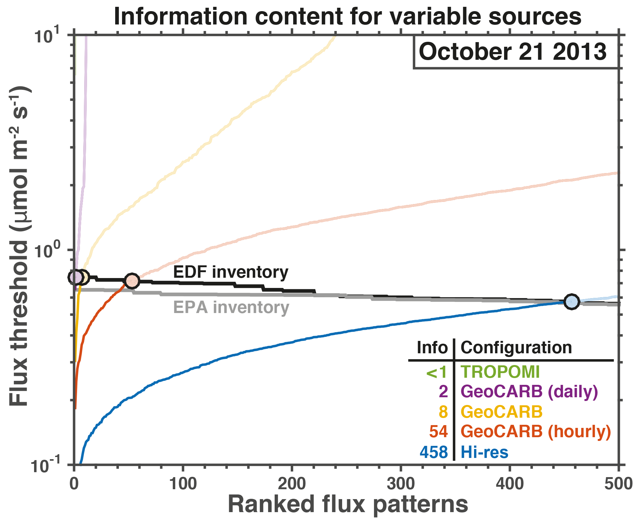
Figure 5Capability of different configurations for satellite observations of atmospheric methane (Table 1) to resolve the fine-scale (1.3 × 1.3 km2) patterns of variability of temporally invariant emissions in a 290 × 235 km2 domain and for a 1-week observation period. The colored lines show the flux thresholds for the different emission patterns of variability in the domain, as given by the ordered inverse square roots of the eigenvalues of the Fisher information matrix. Solid black line is the eigenvalues of the emissions from the EDF Barnett Shale methane inventory (Lyon et al., 2015) and the solid gray line is the gridded EPA inventory. The region above the black line is where the noise is larger than the signal. Filled circles indicate the information content of the observing system (ℐ) for a given satellite configuration at 1.3 × 1.3 km2 spatial resolution. Inset table lists the information contents for the five configurations.
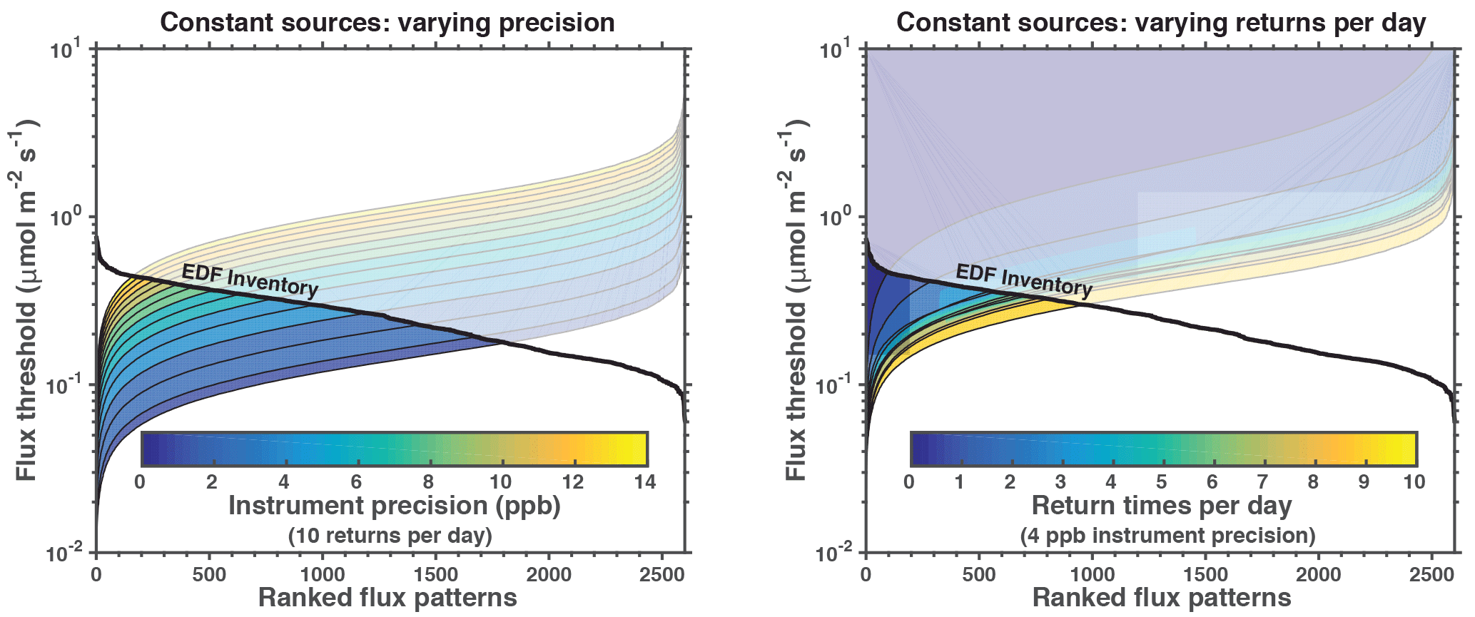
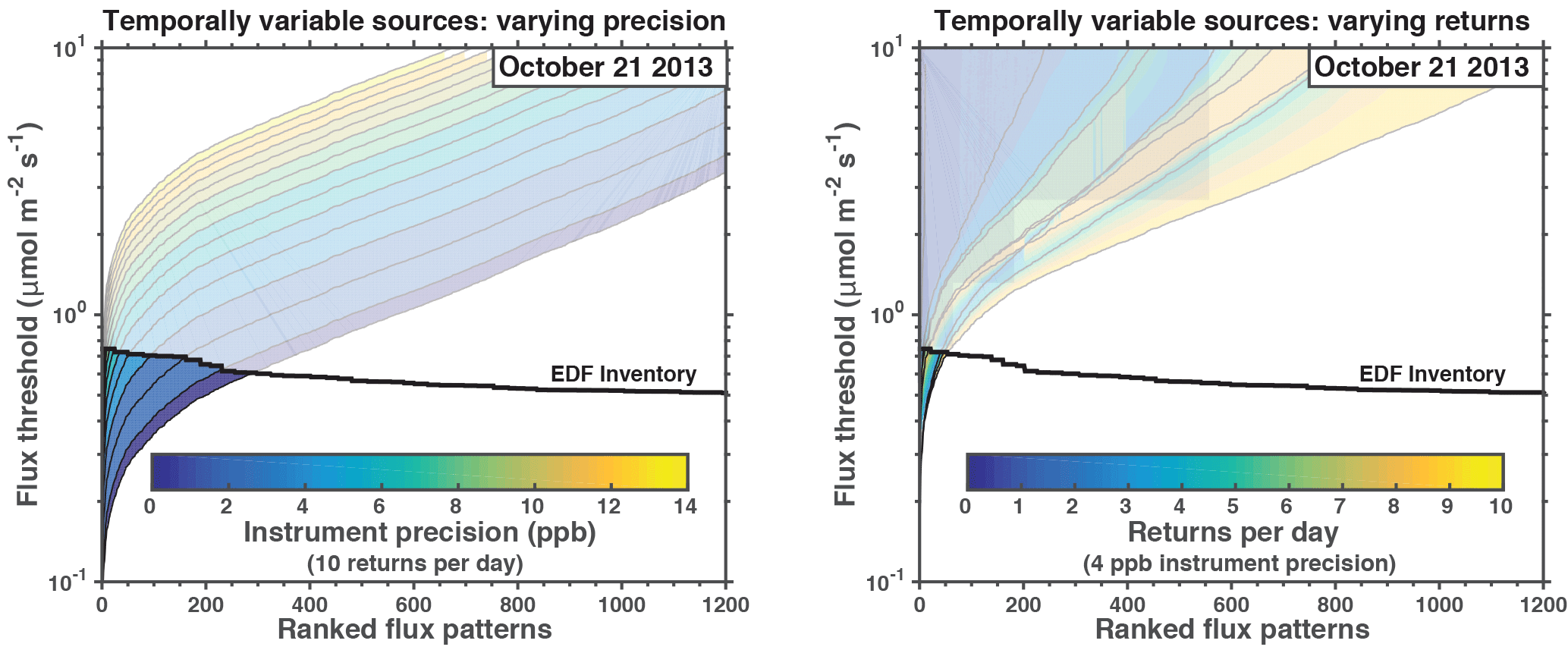
Figure 6Capability of GeoCARB-like satellite configurations to resolve the fine-scale (1.3 × 1.3 km2) patterns of variability of temporally invariant emissions in a 290 × 235 km2 domain and for a 1-week observation period. Left panel shows the results for a configuration with 10 returns per day (hourly observations) where the instrument precision is varied from 0 to 14 ppb. Right panel shows the results for a configuration with 4 ppb instrument precision and the return frequency per day is varied from 1 to 10. Solid black line shows eigenvalues of the EDF Barnett Shale methane emission inventory (Lyon et al., 2015). The region above the black line is where the noise is larger than the signal. The change in flux threshold as the sampling frequency increases in right panel is not necessarily monotonic, because some of the cases use different subsets of observation (e.g., daily observations are at 13:00 LT while twice daily are at 10 and 14).
Figure 5 shows the ensemble of flux thresholds for the five satellite configurations, assuming temporally invariant emissions. The ranked flux patterns are on the abscissa; leading flux patterns correspond to larger patterns of variability (e.g., regional-scale emissions), and the trailing flux patterns correspond to fine-scale variability. The corresponding flux thresholds are on the ordinate. The flux threshold is lowest for the leading flux patterns and largest for the trailing flux patterns. This means that the regional-scale emissions are easiest to quantify and the finer-scale emissions are increasingly difficult to quantify. The information content (ℐ) is obtained from the intersection of the flux thresholds (colored lines) with the eigenvalues from the emission inventory (black line). A higher information content means that finer scales of emission variability can be detected.
From Fig. 5, we see that a week of TROPOMI observations provides five pieces of information on emissions for the 70 × 70 km2 core domain out of a possible 2601 pieces of information describing the emissions on the 1.3 × 1.3 km2 grid. The actual pieces of information are the eigenvectors of the Fisher information matrix, and the ranked eigenvectors describe gradually finer patterns of variability from 70 × 70 to 1.3 × 1.3 km2. The kth ranked eigenvector may be assumed to describe an emission pattern of dimension 70, implying that TROPOMI can resolve emissions on a 30 km scale.
The three GeoCARB configurations provide 98–961 pieces of information dependent on whether the observations are daily, twice daily, or hourly. Following the above assumption, this corresponds to resolving emissions on a ∼ 2–7 km scale. Hourly observations provide 10 times more information (as defined by Eq. 8) on emission patterns than daily observations, and 3 times more than twice-daily observations (the default configuration of GeoCARB). Remarkably, more is gained by going from daily to twice daily (factor of 3.4) than going from twice daily to hourly (factor of 2.9) because of the temporal error correlation in the transport model. The aspirational hi-res satellite configuration provides 2 221 pieces of information on temporally invariant sources, corresponding to 85 % of the flux patterns in the 70 × 70 km2 observation region, which means that much of the spatial variability in the 1.3 × 1.3 km2 emissions in the Barnett Shale is resolved.
Figure 6 further quantifies the importance of instrument precision and return frequency for the GeoCARB pixel resolution of 2.7 × 3.0 km2. It shows the flux thresholds for a set of configurations where the instrument precision is varied from 0 to 14 ppb and the return frequency is varied from 1 to 10 returns per day. We find that instrument precision is more important than return frequency for increasing the information content from the observations.
In Case 2 we assume that the methane sources in individual pixels vary in time on an hourly basis with no correlation from one hour to the next, making the problem generally underdetermined (m<n) for all satellite configurations. Here we aim to determine the ability of the satellite observations to quantify the hourly emissions over the spatial patterns defined by the eigenvectors of 𝓕 and making no assumption as to the persistence of those emissions. We treat each day independently and compute the eigenvalues of the Fisher information matrix for each day. Figure 7 shows the flux thresholds for the five satellite configurations on a representative day. From Fig. 7, we see that TROPOMI is unable to provide any information on hourly emissions in the Barnett Shale. The three GeoCARB configurations provide 2–54 pieces of information. Figure 8 evaluates the impact of sampling frequency and instrument precision for the GeoCARB configurations. As with the temporally invariant case, we find that instrument precision is more important for increasing the information content. The aspirational “hi-res” configuration (shown in Fig. 7) is the only configuration that is able to provide substantial information (458 pieces of information) on temporally variable emissions.
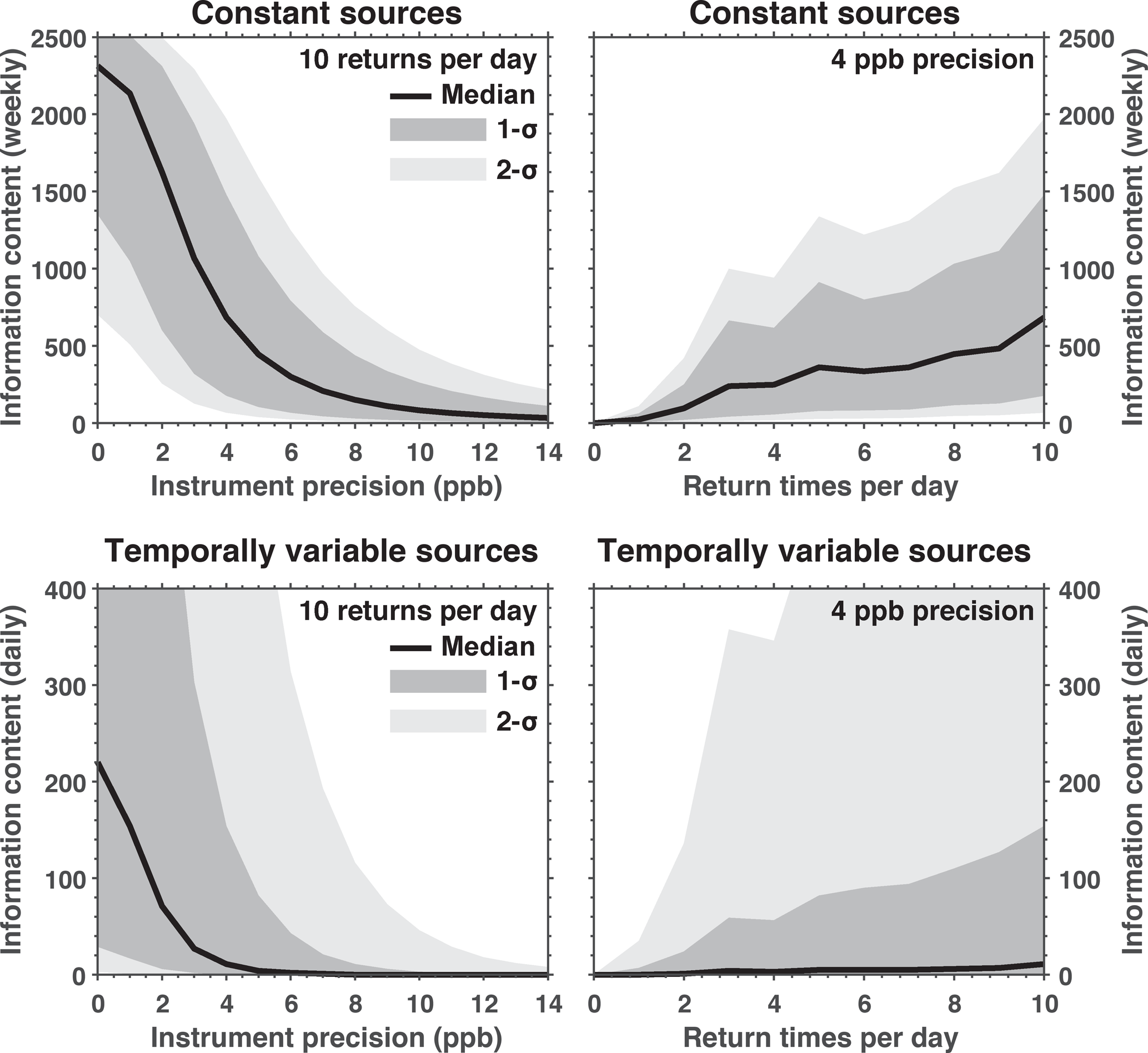
Figure 9Information content ℐ as a function of the instrument precision (left column) and the sampling frequency per day (right column) for a satellite with a pixel resolution of 2.7 × 3.0 km2. Top row is for Case 1 where the sources are assumed to be temporally invariant and bottom row is for Case 2 where the sources are temporally variable. Solid black line is the median information content. A 4 ppb model error is included; see Sect. 3. Uncertainty is from randomly sampling ei from the eigenvalues of the EDF inventory.
Figure 9 summarizes the findings from Figs. 6 and 8. It compares the information content ℐ from configurations with 2.7 × 3.0 km2 spatial resolution (GeoCARB) as the instrument precision and return frequency are varied from 0 to 14 ppb and 1 to 10 returns per day, respectively, for both temporally variable and constant sources. Uncertainty of ℐ is estimated by randomly sampling ei from the ensemble of emission inventory eigenvalues and comparing to fi in Eq. 8. For the temporally invariant sources (Case 1), we find considerable increases in information content for instrument precisions better than 6 ppb (top left panel in Fig. 9) and an approximately linear relationship between information content and return frequency (top right panel in Fig. 9). The satellite configurations provide considerably less information for the temporally variable sources (Case 2). We find that satellite configurations with instrument precision worse than 6 ppb provide no information on temporally variable sources (bottom left panel in Fig. 9). As with the temporally invariant case, we find an approximately linear relationship between information content and return frequency (bottom right panel in Fig. 9). From this, we conclude that a GeoCARB-like instrument would greatly benefit from having an instrument precision better than 6 ppb.
We conducted an observing system simulation experiment (OSSE) to evaluate the potential of different satellite observation systems for atmospheric methane to quantify methane emissions at kilometer scale. This involved a 1-week WRF-STILT simulation of atmospheric methane columns with 1.3 × 1.3 km2 spatial resolution over the 290 × 235 km2 Barnett Shale domain to quantify the information content of different satellite instrument configurations for resolving the kilometer-scale distribution of methane emissions within that domain. We evaluated the information content of the different satellite observing systems through an eigenanalysis of the Fisher information matrix 𝓕, which characterizes the capability of an observing system independently of the form of the prior information. The eigenvalues of 𝓕 define the emission flux thresholds for detection of emission patterns down to 1.3 km in scale as defined by the eigenvectors. Here we put these flux thresholds in context of the high-resolution EDF emission inventory for the Barnett Shale to quantify the information content from different satellite observing configurations. The same approach could be readily used for different observation domains and different prior inventories.
We find from this analysis that the recently launched TROPOMI satellite instrument (low-Earth orbit, 7 × 7 km2 pixels, daily return time, 11 ppb precision) should be able to constrain the mean emissions in the Barnett Shale and provide some coarse-resolution information on the distribution of temporally invariant emissions at ∼ 30 km scales. The planned GeoCARB instrument (geostationary orbit, 2.7 × 3.0 km2 pixels, twice-daily return time, 4 ppb precision) will provide 50 times more information than TROPOMI. The observing frequency of GeoCARB is still under discussion; we find that twice-daily observations triple the information content relative to daily observations, while hourly observations allow another tripling. The 4 ppb precision of GeoCARB is well adapted to the magnitude of methane sources; we find that a precision larger than 6 ppb would considerably decrease the information content. An aspirational “hi-res” instrument using attributes of currently proposed instruments (geostationary orbit, 1.3 × 1.3 km2 pixels, hourly return time, 1 ppb precision) can resolve much of the kilometer-scale spatial distribution in the EDF inventory. This assumes that the emissions are constant in time or that their temporal variability is known. Resolving hourly variable emissions at the kilometer scale will be very limited even with the aspirational “hi-res” instrument.
The source code for all models is publicly available through the cited references.
We treat 𝓕 and B−1 separately because it is computationally infeasible to compute the eigenvalues of the matrix product when we attempt to resolve hourly emissions as n>106 and both 𝓕 and B−1 are n×n matrices. This separation of 𝓕 and B−1 results in our estimate of ℐ likely being an upper bound on the information content. This follows from Bhatia (1997) who prove that , where C and D are Hermitian positive definite matrices, λ↓(X) denotes the vector of eigenvalues of X in decreasing order, ≺w is the weak majorization preorder, and . Therefore, directly computing the eigenvalues of , as Rodgers (2000) suggests for the Bayesian inference case with Gaussian errors, would likely yield fewer eigenvalues larger than unity than our estimate.
In the case of temporally variable emissions, the system is generally underdetermined (m<n) and we can use a singular value decomposition to efficiently compute the eigenvalues of 𝓕. For an m×n real matrix A, the non-zero singular values of ATA and AAT are identical even though the singular vectors are different (see, for example, Rodgers, 2000) but the dimensions of these two matrices are n×n and m×m, respectively, and the eigenvalues can be computed from the square root of the non-zero singular values. We can write , where is the pre-whitened Jacobian and L is a lower triangular matrix from a Cholesky decomposition of R (such that R=LLT). Thus, the eigenvalues of 𝓕 can be obtained by analysis of either (an n×n matrix) or (an m×m matrix).
The authors declare that they have no conflict of interest.
This work was supported by the ExxonMobil Research and Engineering Company
and the US Department of Energy (DOE) Advanced Research Projects Agency –
Energy (ARPA-E). A. J. Turner is supported as a Miller Fellow with the Miller
Institute for Basic Research in Science at UC Berkeley. This research used
the Savio computational cluster resource provided by the Berkeley Research
Computing program at the University of California, Berkeley (supported by the
UC Berkeley Chancellor, Vice Chancellor for Res., and Chief Information
Officer). This research also used resources from the National Energy Research
Scientific Computing Center, which is supported by the Office of Science of
the DOE under contract no. DE-AC02-05CH11231. We also
acknowledge high-performance computing support from Cheyenne
(doi:10.5065/D6RX99HX) provided by NCAR's Computational and Information
Systems Laboratory, sponsored by the National Science
Foundation.
Edited by: Martin
Heimann
Reviewed by: two anonymous referees
Alexe, M., Bergamaschi, P., Segers, A., Detmers, R., Butz, A., Hasekamp, O., Guerlet, S., Parker, R., Boesch, H., Frankenberg, C., Scheepmaker, R. A., Dlugokencky, E., Sweeney, C., Wofsy, S. C., and Kort, E. A.: Inverse modelling of CH4 emissions for 2010–2011 using different satellite retrieval products from GOSAT and SCIAMACHY, Atmos. Chem. Phys., 15, 113–133, https://doi.org/10.5194/acp-15-113-2015, 2015. a
Bergamaschi, P., Frankenberg, C., Meirink, J. F., Krol, M., Villani, M. G., Houweling, S., Dentener, F., Dlugokencky, E. J., Miller, J. B., Gatti, L. V., Engel, A., and Levin, I.: Inverse modeling of global and regional CH4 emissions using SCIAMACHY satellite retrievals, J. Geophys. Res., 114, https://doi.org/10.1029/2009jd012287, 2009. a
Bergamaschi, P., Houweling, S., Segers, A., Krol, M., Frankenberg, C., Scheepmaker, R. A., Dlugokencky, E., Wofsy, S. C., Kort, E. A., Sweeney, C., Schuck, T., Brenninkmeijer, C., Chen, H., Beck, V., and Gerbig, C.: Atmospheric CH4 in the first decade of the 21st century: Inverse modeling analysis using SCIAMACHY satellite retrievals and NOAA surface measurements, J. Geophys. Res.-Atmos., 118, 7350–7369, https://doi.org/10.1002/jgrd.50480, 2013. a
Bhatia, R.: Matrix Analysis, Graduate Texts in Mathematics, Springer, New York, 1997. a
Bousserez, N., Henze, D. K., Rooney, B., Perkins, A., Wecht, K. J., Turner, A. J., Natraj, V., and Worden, J. R.: Constraints on methane emissions in North America from future geostationary remote-sensing measurements, Atmos. Chem. Phys., 16, 6175–6190, https://doi.org/10.5194/acp-16-6175-2016, 2016. a
Bovensmann, H., Buchwitz, M., Burrows, J. P., Reuter, M., Krings, T., Gerilowski, K., Schneising, O., Heymann, J., Tretner, A., and Erzinger, J.: A remote sensing technique for global monitoring of power plant CO2 emissions from space and related applications, Atmos. Meas. Tech., 3, 781–811, https://doi.org/10.5194/amt-3-781-2010, 2010. a, b
Brandt, A. R., Heath, G. A., Kort, E. A., O'Sullivan, F., Petron, G., Jordaan, S. M., Tans, P., Wilcox, J., Gopstein, A. M., Arent, D., Wofsy, S., Brown, N. J., Bradley, R., Stucky, G. D., Eardley, D., and Harriss, R.: Energy and environment. Methane leaks from North American natural gas systems, Science, 343, 733–735, https://doi.org/10.1126/science.1247045, 2014. a
Brasseur, G. P. and Jacob, D. J.: Modeling of Atmospheric Chemistry, Princeton University Press, Princeton, NJ, 2017. a
Buchwitz, M., Reuter, M., Schneising, O., Boesch, H., Guerlet, S., Dils, B., Aben, I., Armante, R., Bergamaschi, P., Blumenstock, T., Bovensmann, H., Brunner, D., Buchmann, B., Burrows, J. P., Butz, A., Chédin, A., Chevallier, F., Crevoisier, C. D., Deutscher, N. M., Frankenberg, C., Hase, F., Hasekamp, O. P., Heymann, J., Kaminski, T., Laeng, A., Lichtenberg, G., De Maziére, M., Noël, S., Notholt, J., Orphal, J., Popp, C., Parker, R., Scholze, M., Sussmann, R., Stiller, G. P., Warneke, T., Zehner, C., Bril, A., Crisp, D., Griffith, D. W. T., Kuze, A., O'Dell, C., Oshchepkov, S., Sherlock, V., Suto, H., Wennberg, P., Wunch, D., Yokota, T., and Yoshida, Y.: The Greenhouse Gas Climate Change Initiative (GHG-CCI): Comparison and quality assessment of near-surface-sensitive satellite-derived CO2 and CH4 global data sets, Remote Sens. Environ., 162, 344–362, https://doi.org/10.1016/j.rse.2013.04.024, 2015. a
Buchwitz, M., Schneising, O., Reuter, M., Heymann, J., Krautwurst, S., Bovensmann, H., Burrows, J. P., Boesch, H., Parker, R. J., Somkuti, P., Detmers, R. G., Hasekamp, O. P., Aben, I., Butz, A., Frankenberg, C., and Turner, A. J.: Satellite-derived methane hotspot emission estimates using a fast data-driven method, Atmos. Chem. Phys., 17, 5751–5774, https://doi.org/10.5194/acp-17-5751-2017, 2017. a
Butz, A., Galli, A., Hasekamp, O., Landgraf, J., Tol, P., and Aben, I.: TROPOMI aboard Sentinel-5 Precursor: Prospective performance of CH4 retrievals for aerosol and cirrus loaded atmospheres, Remote Sens. Environ., 120, 267–276, https://doi.org/10.1016/j.rse.2011.05.030, 2012. a
Butz, A., Orphal, J., Checa-Garcia, R., Friedl-Vallon, F., von Clarmann, T., Bovensmann, H., Hasekamp, O., Landgraf, J., Knigge, T., Weise, D., Sqalli-Houssini, O., and Kemper, D.: Geostationary Emission Explorer for Europe (G3E): mission concept and initial performance assessment, Atmos. Meas. Tech., 8, 4719–4734, https://doi.org/10.5194/amt-8-4719-2015, 2015. a
Candes, E. J. and Wakin, M. B.: An introduction to compressive sampling, IEEE Signal Processing Magazine, 25, 21–30, https://doi.org/10.1109/Msp.2007.914731, 2008. a
Caulton, D. R., Shepson, P. B., Santoro, R. L., Sparks, J. P., Howarth, R. W., Ingraffea, A. R., Cambaliza, M. O., Sweeney, C., Karion, A., Davis, K. J., Stirm, B. H., Montzka, S. A., and Miller, B. R.: Toward a better understanding and quantification of methane emissions from shale gas development, P. Natl. Acad. Sci. USA, 111, https://doi.org/10.1073/pnas.1316546111, 2014. a
Conley, S., Franco, G., Faloona, I., Blake, D. R., Peischl, J., and Ryerson, T. B.: Methane emissions from the 2015 Aliso Canyon blowout in Los Angeles, CA, Science, 351, 1317–20, https://doi.org/10.1126/science.aaf2348, 2016. a
Cressot, C., Chevallier, F., Bousquet, P., Crevoisier, C., Dlugokencky, E. J., Fortems-Cheiney, A., Frankenberg, C., Parker, R., Pison, I., Scheepmaker, R. A., Montzka, S. A., Krummel, P. B., Steele, L. P., and Langenfelds, R. L.: On the consistency between global and regional methane emissions inferred from SCIAMACHY, TANSO-FTS, IASI and surface measurements, Atmos. Chem. Phys., 14, 577–592, https://doi.org/10.5194/acp-14-577-2014, 2014. a
Fishman, J., Iraci, L. T., Al-Saadi, J., Chance, K., Chavez, F., Chin, M., Coble, P., Davis, C., DiGiacomo, P. M., Edwards, D., Eldering, A., Goes, J., Herman, J., Hu, C., Jacob, D. J., Jordan, C., Kawa, S. R., Key, R., Liu, X., Lohrenz, S., Mannino, A., Natraj, V., Neil, D., Neu, J., Newchurch, M., Pickering, K., Salisbury, J., Sosik, H., Subramaniam, A., Tzortziou, M., Wang, J., and Wang, M.: The United States' Next Generation of Atmospheric Composition and Coastal Ecosystem Measurements: NASA's Geostationary Coastal and Air Pollution Events (GEO-CAPE) Mission, B. Am. Meteorol. Soc., 93, 1547–1566, https://doi.org/10.1175/bams-d-11-00201.1, 2012. a, b
Frankenberg, C., Meirink, J. F., van Weele, M., Platt, U., and Wagner, T.: Assessing methane emissions from global space-borne observations, Science, 308, 1010–1014, https://doi.org/10.1126/science.1106644, 2005. a
Frankenberg, C., Thorpe, A. K., Thompson, D. R., Hulley, G., Kort, E. A., Vance, N., Borchardt, J., Krings, T., Gerilowski, K., Sweeney, C., Conley, S., Bue, B. D., Aubrey, A. D., Hook, S., and Green, R. O.: Airborne methane remote measurements reveal heavy-tail flux distribution in Four Corners region, P. Natl. Acad. Sci. USA, 113, 9734–9739, https://doi.org/10.1073/pnas.1605617113, 2016. a
Fraser, A., Palmer, P. I., Feng, L., Boesch, H., Cogan, A., Parker, R., Dlugokencky, E. J., Fraser, P. J., Krummel, P. B., Langenfelds, R. L., O'Doherty, S., Prinn, R. G., Steele, L. P., van der Schoot, M., and Weiss, R. F.: Estimating regional methane surface fluxes: the relative importance of surface and GOSAT mole fraction measurements, Atmos. Chem. Phys., 13, 5697–5713, https://doi.org/10.5194/acp-13-5697-2013, 2013. a
Houweling, S., Bergamaschi, P., Chevallier, F., Heimann, M., Kaminski, T., Krol, M., Michalak, A. M., and Patra, P.: Global inverse modeling of CH4 sources and sinks: an overview of methods, Atmos. Chem. Phys., 17, 235–256, https://doi.org/10.5194/acp-17-235-2017, 2017. a
Hu, H., Hasekamp, O., Butz, A., Galli, A., Landgraf, J., Aan de Brugh, J., Borsdorff, T., Scheepmaker, R., and Aben, I.: The operational methane retrieval algorithm for TROPOMI, Atmos. Meas. Tech., 9, 5423–5440, https://doi.org/10.5194/amt-9-5423-2016, 2016. a
Hu, H., Landgraf, J., Detmers, R., Borsdorff, T., Aan de Brugh, J., Aben, I., Butz, A., and Hasekamp, O.: Toward Global Mapping of Methane With TROPOMI: First Results and Intersatellite Comparison to GOSAT, Geophys. Res. Lett., 45, https://doi.org/10.1002/2018gl077259, 2018. a
Jacob, D. J., Turner, A. J., Maasakkers, J. D., Sheng, J., Sun, K., Liu, X., Chance, K., Aben, I., McKeever, J., and Frankenberg, C.: Satellite observations of atmospheric methane and their value for quantifying methane emissions, Atmos. Chem. Phys., 16, 14371–14396, https://doi.org/10.5194/acp-16-14371-2016, 2016. a, b
Karion, A., Sweeney, C., Pétron, G., Frost, G., Michael Hardesty, R., Kofler, J., Miller, B. R., Newberger, T., Wolter, S., Banta, R., Brewer, A., Dlugokencky, E., Lang, P., Montzka, S. A., Schnell, R., Tans, P., Trainer, M., Zamora, R., and Conley, S.: Methane emissions estimate from airborne measurements over a western United States natural gas field, Geophys. Res. Lett., 40, 4393–4397, https://doi.org/10.1002/grl.50811, 2013. a
Karion, A., Sweeney, C., Kort, E. A., Shepson, P. B., Brewer, A., Cambaliza, M., Conley, S. A., Davis, K., Deng, A., Hardesty, M., Herndon, S. C., Lauvaux, T., Lavoie, T., Lyon, D., Newberger, T., Petron, G., Rella, C., Smith, M., Wolter, S., Yacovitch, T. I., and Tans, P.: Aircraft-Based Estimate of Total Methane Emissions from the Barnett Shale Region, Environ. Sci. Technol., 49, 8124–31, https://doi.org/10.1021/acs.est.5b00217, 2015. a
Kirschke, S., Bousquet, P., Ciais, P., Saunois, M., Canadell, J. G., Dlugokencky, E. J., Bergamaschi, P., Bergmann, D., Blake, D. R., Bruhwiler, L., Cameron-Smith, P., Castaldi, S., Chevallier, F., Feng, L., Fraser, A., Heimann, M., Hodson, E. L., Houweling, S., Josse, B., Fraser, P. J., Krummel, P. B., Lamarque, J.-F., Langenfelds, R. L., Le Quéré, C., Naik, V., O'Doherty, S., Palmer, P. I., Pison, I., Plummer, D., Poulter, B., Prinn, R. G., Rigby, M., Ringeval, B., Santini, M., Schmidt, M., Shindell, D. T., Simpson, I. J., Spahni, R., Steele, L. P., Strode, S. A., Sudo, K., Szopa, S., van der Werf, G. R., Voulgarakis, A., van Weele, M., Weiss, R. F., Williams, J. E., and Zeng, G.: Three decades of global methane sources and sinks, Nat. Geosci., 6, 813–823, https://doi.org/10.1038/ngeo1955, 2013. a
Kort, E. A., Frankenberg, C., Costigan, K. R., Lindenmaier, R., Dubey, M. K., and Wunch, D.: Four corners: The largest US methane anomaly viewed from space, Geophys. Res. Lett., 41, https://doi.org/10.1002/2014gl061503, 2014. a
Kuze, A., Suto, H., Nakajima, M., and Hamazaki, T.: Thermal and near infrared sensor for carbon observation Fourier-transform spectrometer on the Greenhouse Gases Observing Satellite for greenhouse gases monitoring, Appl. Opt., 48, 6716–6733, https://doi.org/10.1364/AO.48.006716, 2009. a
Kuze, A., Suto, H., Shiomi, K., Kawakami, S., Tanaka, M., Ueda, Y., Deguchi, A., Yoshida, J., Yamamoto, Y., Kataoka, F., Taylor, T. E., and Buijs, H. L.: Update on GOSAT TANSO-FTS performance, operations, and data products after more than 6 years in space, Atmos. Meas. Tech., 9, 2445–2461, https://doi.org/10.5194/amt-9-2445-2016, 2016. a
Lavoie, T. N., Shepson, P. B., Cambaliza, M. O., Stirm, B. H., Karion, A., Sweeney, C., Yacovitch, T. I., Herndon, S. C., Lan, X., and Lyon, D.: Aircraft-Based Measurements of Point Source Methane Emissions in the Barnett Shale Basin, Environ. Sci. Technol., 49, 7904–7913, https://doi.org/10.1021/acs.est.5b00410, 2015. a
Lin, J. C., Gerbig, C., Wofsy, S. C., Andrews, A. E., Daube, B. C., Davis, K. J., and Grainger, C. A.: A near-field tool for simulating the upstream influence of atmospheric observations: The Stochastic Time-Inverted Lagrangian Transport (STILT) model, J. Geophys. Res.-Atmos., 108, ACH 2–1–ACH 2–17, https://doi.org/10.1029/2002jd003161, 2003. a
Lyon, D. R., Zavala-Araiza, D., Alvarez, R. A., Harriss, R., Palacios, V., Lan, X., Talbot, R., Lavoie, T., Shepson, P., Yacovitch, T. I., Herndon, S. C., Marchese, A. J., Zimmerle, D., Robinson, A. L., and Hamburg, S. P.: Constructing a Spatially Resolved Methane Emission Inventory for the Barnett Shale Region, Environ. Sci. Tech., 49, 8147–8157, https://doi.org/10.1021/es506359c, 2015. a, b, c, d, e, f
Maasakkers, J. D., Jacob, D. J., Sulprizio, M. P., Turner, A. J., Weitz, M., Wirth, T., Hight, C., DeFigueiredo, M., Desai, M., Schmeltz, R., Hockstad, L., Bloom, A. A., Bowman, K. W., Jeong, S., and Fischer, M. L.: Gridded National Inventory of U.S. Methane Emissions, Environ. Sci. Tech., 50, 13123–13133, https://doi.org/10.1021/acs.est.6b02878, 2016. a, b, c
Miller, S. M., Wofsy, S. C., Michalak, A. M., Kort, E. A., Andrews, A. E., Biraud, S. C., Dlugokencky, E. J., Eluszkiewicz, J., Fischer, M. L., Janssens-Maenhout, G., Miller, B. R., Miller, J. B., Montzka, S. A., Nehrkorn, T., and Sweeney, C.: Anthropogenic emissions of methane in the United States, P. Natl. Acad. Sci. USA, 110, 20018–20022, https://doi.org/10.1073/pnas.1314392110, 2013. a
Monteil, G., Houweling, S., Butz, A., Guerlet, S., Schepers, D., Hasekamp, O., Frankenberg, C., Scheepmaker, R., Aben, I., and Röckmann, T.: Comparison of CH4 inversions based on 15 months of GOSAT and SCIAMACHY observations, J. Geophys. Res.-Atmos., 118, 11807–11823, https://doi.org/10.1002/2013jd019760, 2013. a
O'Brien, D. M., Polonsky, I. N., Utembe, S. R., and Rayner, P. J.: Potential of a geostationary geoCARB mission to estimate surface emissions of CO2, CH4 and CO in a polluted urban environment: case study Shanghai, Atmos. Meas. Tech., 9, 4633–4654, https://doi.org/10.5194/amt-9-4633-2016, 2016. a, b
O'Dell, C. W., Connor, B., Bösch, H., O'Brien, D., Frankenberg, C., Castano, R., Christi, M., Eldering, D., Fisher, B., Gunson, M., McDuffie, J., Miller, C. E., Natraj, V., Oyafuso, F., Polonsky, I., Smyth, M., Taylor, T., Toon, G. C., Wennberg, P. O., and Wunch, D.: The ACOS CO2 retrieval algorithm – Part 1: Description and validation against synthetic observations, Atmos. Meas. Tech., 5, 99–121, https://doi.org/10.5194/amt-5-99-2012, 2012. a
Peischl, J., Ryerson, T. B., Aikin, K. C., de Gouw, J. A., Gilman, J. B., Holloway, J. S., Lerner, B. M., Nadkarni, R., Neuman, J. A., Nowak, J. B., Trainer, M., Warneke, C., and Parrish, D. D.: Quantifying atmospheric methane emissions from the Haynesville, Fayetteville, and northeastern Marcellus shale gas production regions, J. Geophys. Res.-Atmos., 120, 2119–2139, https://doi.org/10.1002/2014JD022697, 2015. a
Peischl, J., Karion, A., Sweeney, C., Kort, E. A., Smith, M. L., Brandt, A. R., Yeskoo, T., Aikin, K. C., Conley, S. A., Gvakharia, A., Trainer, M., Wolter, S., and Ryerson, T. B.: Quantifying atmospheric methane emissions from oil and natural gas production in the Bakken shale region of North Dakota, J. Geophys. Res.-Atmos., 121, 6101–6111, https://doi.org/10.1002/2015jd024631, 2016. a
Polonsky, I. N., O'Brien, D. M., Kumer, J. B., O'Dell, C. W., and the geoCARB Team: Performance of a geostationary mission, geoCARB, to measure CO2, CH4 and CO column-averaged concentrations, Atmos. Meas. Tech., 7, 959–981, https://doi.org/10.5194/amt-7-959-2014, 2014. a
Rayner, P. J., Utembe, S. R., and Crowell, S.: Constraining regional greenhouse gas emissions using geostationary concentration measurements: a theoretical study, Atmos. Meas. Tech., 7, 3285–3293, https://doi.org/10.5194/amt-7-3285-2014, 2014. a
Rodgers, C. D.: Inverse Methods for Atmospheric Sounding, World Scientific, Singapore, 2000. a, b, c, d
Saunois, M., Bousquet, P., Poulter, B., Peregon, A., Ciais, P., Canadell, J. G., Dlugokencky, E. J., Etiope, G., Bastviken, D., Houweling, S., Janssens-Maenhout, G., Tubiello, F. N., Castaldi, S., Jackson, R. B., Alexe, M., Arora, V. K., Beerling, D. J., Bergamaschi, P., Blake, D. R., Brailsford, G., Brovkin, V., Bruhwiler, L., Crevoisier, C., Crill, P., Covey, K., Curry, C., Frankenberg, C., Gedney, N., Höglund-Isaksson, L., Ishizawa, M., Ito, A., Joos, F., Kim, H.-S., Kleinen, T., Krummel, P., Lamarque, J.-F., Langenfelds, R., Locatelli, R., Machida, T., Maksyutov, S., McDonald, K. C., Marshall, J., Melton, J. R., Morino, I., Naik, V., O'Doherty, S., Parmentier, F.-J. W., Patra, P. K., Peng, C., Peng, S., Peters, G. P., Pison, I., Prigent, C., Prinn, R., Ramonet, M., Riley, W. J., Saito, M., Santini, M., Schroeder, R., Simpson, I. J., Spahni, R., Steele, P., Takizawa, A., Thornton, B. F., Tian, H., Tohjima, Y., Viovy, N., Voulgarakis, A., van Weele, M., van der Werf, G. R., Weiss, R., Wiedinmyer, C., Wilton, D. J., Wiltshire, A., Worthy, D., Wunch, D., Xu, X., Yoshida, Y., Zhang, B., Zhang, Z., and Zhu, Q.: The global methane budget 2000–2012, Earth Syst. Sci. Data, 8, 697–751, https://doi.org/10.5194/essd-8-697-2016, 2016. a
Sheng, J.-X., Jacob, D. J., Turner, A. J., Maasakkers, J. D., Benmergui, J., Bloom, A. A., Arndt, C., Gautam, R., Zavala-Araiza, D., Boesch, H., and Parker, R. J.: 2010–2015 methane trends over Canada, the United States, and Mexico observed by the GOSAT satellite: contributions from different source sectors, Atmos. Chem. Phys. Discuss., https://doi.org/10.5194/acp-2017-1110, in review, 2018a. a
Sheng, J.-X., Jacob, D. J., Turner, A. J., Maasakkers, J. D., Sulprizio, M. P., Bloom, A. A., Andrews, A. E., and Wunch, D.: High-resolution inversion of methane emissions in the Southeast US using SEAC4RS aircraft observations of atmospheric methane: anthropogenic and wetland sources, Atmos. Chem. Phys., 18, 6483–6491, https://doi.org/10.5194/acp-18-6483-2018, 2018b. a, b
Skamarock, W. C., Klemp, J. B., Dudhia, J., Gill, D. O., Barker, D. M., Duda, M. G., Huang, X.-Y., Wang, W., and Powers, J. G.: A Description of the Advanced Research WRF Version 3, Tech. rep., National Center for Atmospheric Res., https://doi.org/10.5065/D68S4MVH, 2008. a, b
Tan, Z., Zhuang, Q., Henze, D. K., Frankenberg, C., Dlugokencky, E., Sweeney, C., Turner, A. J., Sasakawa, M., and Machida, T.: Inverse modeling of pan-Arctic methane emissions at high spatial resolution: what can we learn from assimilating satellite retrievals and using different process-based wetland and lake biogeochemical models?, Atmos. Chem. Phys., 16, 12649–12666, https://doi.org/10.5194/acp-16-12649-2016, 2016. a
Tarantola, A.: Inverse Problem Theory and Methods for Model Parameter Estimation, Society for Industrial and Applied Mathematics, Philadelphia, PA, USA, 2004. a
Turner, A. J. and Jacob, D. J.: Balancing aggregation and smoothing errors in inverse models, Atmos. Chem. Phys., 15, 7039–7048, https://doi.org/10.5194/acp-15-7039-2015, 2015. a
Turner, A. J., Jacob, D. J., Wecht, K. J., Maasakkers, J. D., Lundgren, E., Andrews, A. E., Biraud, S. C., Boesch, H., Bowman, K. W., Deutscher, N. M., Dubey, M. K., Griffith, D. W. T., Hase, F., Kuze, A., Notholt, J., Ohyama, H., Parker, R., Payne, V. H., Sussmann, R., Sweeney, C., Velazco, V. A., Warneke, T., Wennberg, P. O., and Wunch, D.: Estimating global and North American methane emissions with high spatial resolution using GOSAT satellite data, Atmos. Chem. Phys., 15, 7049–7069, https://doi.org/10.5194/acp-15-7049-2015, 2015. a
Turner, A. J., Jacob, D. J., Benmergui, J., Wofsy, S. C., Maasakkers, J. D., Butz, A., Hasekamp, O., and Biraud, S. C.: A large increase in U.S. methane emissions over the past decade inferred from satellite data and surface observations, Geophys. Res. Lett., 2218–2224, https://doi.org/10.1002/2016gl067987, 2016a. a
Turner, A. J., Shusterman, A. A., McDonald, B. C., Teige, V., Harley, R. A., and Cohen, R. C.: Network design for quantifying urban CO2 emissions: assessing trade-offs between precision and network density, Atmos. Chem. Phys., 16, 13465–13475, https://doi.org/10.5194/acp-16-13465-2016, 2016b. a, b
Turner, A. J., Frankenberg, C., Wennberg, P. O., and Jacob, D. J.: Ambiguity in the causes for decadal trends in atmospheric methane and hydroxyl, P. Natl. Acad. Sci. USA, 114, 5367–5372, https://doi.org/10.1073/pnas.1616020114, 2017. a
Veefkind, J. P., Aben, I., McMullan, K., Förster, H., de Vries, J., Otter, G., Claas, J., Eskes, H. J., de Haan, J. F., Kleipool, Q., van Weele, M., Hasekamp, O., Hoogeveen, R., Landgraf, J., Snel, R., Tol, P., Ingmann, P., Voors, R., Kruizinga, B., Vink, R., Visser, H., and Levelt, P. F.: TROPOMI on the ESA Sentinel-5 Precursor: A GMES mission for global observations of the atmospheric composition for climate, air quality and ozone layer applications, Remote Sens. Environ., 120, 70–83, https://doi.org/10.1016/j.rse.2011.09.027, 2012. a, b
Wecht, K. J., Jacob, D. J., Frankenberg, C., Jiang, Z., and Blake, D. R.: Mapping of North American methane emissions with high spatial resolution by inversion of SCIAMACHY satellite data, J. Geophys. Res.-Atmos., 119, 7741–7756, https://doi.org/10.1002/2014jd021551, 2014a. a
Wecht, K. J., Jacob, D. J., Sulprizio, M. P., Santoni, G. W., Wofsy, S. C., Parker, R., Bösch, H., and Worden, J.: Spatially resolving methane emissions in California: constraints from the CalNex aircraft campaign and from present (GOSAT, TES) and future (TROPOMI, geostationary) satellite observations, Atmos. Chem. Phys., 14, 8173–8184, https://doi.org/10.5194/acp-14-8173-2014, 2014b. a
Worden, J. R., Turner, A. J., Bloom, A., Kulawik, S. S., Liu, J., Lee, M., Weidner, R., Bowman, K., Frankenberg, C., Parker, R., and Payne, V. H.: Quantifying lower tropospheric methane concentrations using GOSAT near-IR and TES thermal IR measurements, Atmos. Meas. Tech., 8, 3433–3445, https://doi.org/10.5194/amt-8-3433-2015, 2015. a
Xi, X., Natraj, V., Shia, R. L., Luo, M., Zhang, Q., Newman, S., Sander, S. P., and Yung, Y. L.: Simulated retrievals for the remote sensing of CO2, CH4, CO, and H2O from geostationary orbit, Atmos. Meas. Tech., 8, 4817–4830, https://doi.org/10.5194/amt-8-4817-2015, 2015 a, b
Zavala-Araiza, D., Lyon, D. R., Alvarez, R. A., Davis, K. J., Harriss, R., Herndon, S. C., Karion, A., Kort, E. A., Lamb, B. K., Lan, X., Marchese, A. J., Pacala, S. W., Robinson, A. L., Shepson, P. B., Sweeney, C., Talbot, R., Townsend-Small, A., Yacovitch, T. I., Zimmerle, D. J., and Hamburg, S. P.: Reconciling divergent estimates of oil and gas methane emissions, P. Natl. Acad. Sci. USA, 112, 15597–155602, https://doi.org/10.1073/pnas.1522126112, 2015. a, b