the Creative Commons Attribution 4.0 License.
the Creative Commons Attribution 4.0 License.
 | 13 Jun 2018
Top–down quantification of NOx emissions from traffic in an urban area using a high-resolution regional atmospheric chemistry model
Friderike Kuik
Andreas Kerschbaumer
Axel Lauer
Aurelia Lupascu
Erika von Schneidemesser
Tim M. Butler
With NO2 limit values being frequently exceeded in European cities, complying with the European air quality regulations still poses a problem for many cities. Traffic is typically a major source of NOx emissions in urban areas. High-resolution chemistry transport modelling can help to assess the impact of high urban NOx emissions on air quality inside and outside of urban areas. However, many modelling studies report an underestimation of modelled NOx and NO2 compared with observations. Part of this model bias has been attributed to an underestimation of NOx emissions, particularly in urban areas. This is consistent with recent measurement studies quantifying underestimations of urban NOx emissions by current emission inventories, identifying the largest discrepancies when the contribution of traffic NOx emissions is high. This study applies a high-resolution chemistry transport model in combination with ambient measurements in order to assess the potential underestimation of traffic NOx emissions in a frequently used emission inventory. The emission inventory is based on officially reported values and the Berlin–Brandenburg area in Germany is used as a case study. The WRF-Chem model is used at a 3 km × 3 km horizontal resolution, simulating the whole year of 2014. The emission data are downscaled from an original resolution of ca. 7 km × 7 km to a resolution of 1 km × 1 km. An in-depth model evaluation including spectral decomposition of observed and modelled time series and error apportionment suggests that an underestimation in traffic emissions is likely one of the main causes of the bias in modelled NO2 concentrations in the urban background, where NO2 concentrations are underestimated by ca. 8 µg m−3 (−30 %) on average over the whole year. Furthermore, a diurnal cycle of the bias in modelled NO2 suggests that a more realistic treatment of the diurnal cycle of traffic emissions might be needed. Model problems in simulating the correct mixing in the urban planetary boundary layer probably play an important role in contributing to the model bias, particularly in summer. Also taking into account this and other possible sources of model bias, a correction factor for traffic NOx emissions of ca. 3 is estimated for weekday daytime traffic emissions in the core urban area, which corresponds to an overall underestimation of traffic NOx emissions in the core urban area of ca. 50 %. Sensitivity simulations for the months of January and July using the calculated correction factor show that the weekday model bias can be improved from −8.8 µg m−3 (−26 %) to −5.4 µg m−3 (−16 %) in January on average in the urban background, and −10.3 µg m−3 (−46 %) to −7.6 µg m−3 (−34 %) in July. In addition, the negative bias of weekday NO2 concentrations downwind of the city in the rural and suburban background can be reduced from −3.4 µg m−3 (−12 %) to −1.2 µg m−3 (−4 %) in January and from −3.0 µg m−3 (−22 %) to −1.9 µg m−3 (−14 %) in July. The results and their consistency with findings from other studies suggest that more research is needed in order to more accurately understand the spatial and temporal variability in real-world NOx emissions from traffic, and apply this understanding to the inventories used in high-resolution chemical transport models.
- Article
(1244 KB) -
Supplement
(678 KB) - BibTeX
- EndNote


Limit values for ambient NO2 concentrations (Ambient Air Quality Directive 2008/50/EC) as well as NOx exhaust emission standards are set by European legislation, but ambient measurements show that NO2 concentrations still frequently exceed the European annual mean limit value of 40 µg m−3 (EEA, 2016; Minkos et al., 2017). For example, 12 % of all measurement sites in Europe registered exceedances of the annual mean limit value in 2014, most of them located at the roadside. Within Europe, Germany had the highest median NO2 concentrations in 2014 (EEA, 2016), where it was estimated that the limit value was exceeded at 57 % of all traffic sites (Minkos et al., 2017). While there is a downward trend in NO2 concentrations due to decreasing NOx emissions, extrapolating the current trend to 2020, exceedances are still expected at 7 % of the stations in 2020, requiring additional measures in order for the European air quality goals to be met (EEA, 2016).
In general, traffic is the most important source of NOx emissions in Europe, contributing 46 % in 2014 in the EU-28, with considerably higher contributions to ambient NO2 concentrations in urban areas (EEA, 2016). NOx emissions from diesel vehicles, the main traffic NOx source, have recently been a strong focus of international media attention: despite increasingly strict emission standards for diesel cars with the introduction of the Euro 5 and Euro 6 norms, under real-world driving conditions, i.e. the pollutants a car produces while being driven on real roads as opposed to being tested in a lab, Euro 5-certified cars exceed the emission limit of 0.18 g km−1 by an average factor of 4–5 (e.g. EEA, 2016; Hausberger and Matzer, 2017) and the newer Euro 6 cars exceed the emission limit of 0.08 g km−1 by an average factor of 6–7 (e.g. EEA, 2016; ICCT Briefing, 2016).
NOx impacts human health, ecosystems and climate directly and indirectly as a precursor of tropospheric ozone (O3) and particulate matter (PM). Health impacts of NO2 include adverse respiratory effects (WHO, 2013), and the effect of road traffic NO2 on premature mortality might be more than 10 times larger than the effect of road traffic PM2.5 (Harrison and Beddows, 2017).
In order to support policy makers in identifying suitable measures to reduce roadside and urban background NO2 concentrations to levels well below the limit value, as well as to assess the health impact of current and future NO2 concentrations, air pollution modelling is a valuable tool (e.g. von Schneidemesser et al., 2017). Chemistry transport models can be used to assess the impact of local emissions on air chemistry and air quality in the surroundings and downwind of the emission sources. Online-coupled models, such as the chemistry version of the Weather Research and Forecasting model (WRF-Chem, Grell et al., 2005), have several advantages compared with offline approaches. These include, for example, a numerically more consistent treatment and a more realistic representation of the atmosphere, particularly in case of high model resolution (Grell and Baklanov, 2011).
Due to its short lifetime in the atmosphere, NO2 is more spatially variable than for example O3, particularly in urban areas with locally high NOx emissions. This is one of the reasons why models with higher spatial resolutions of a few kilometres are capable of representing observed NO2 concentrations better than coarser models, with better performance if emission input and meteorological data are also available at the high resolution (e.g. Schaap et al., 2015). In terms of model evaluation, comparing NO2 concentrations averaged over a coarse model grid cell with point measurements can lead to mismatches (Solazzo et al., 2017), with a better comparability achieved through high model resolutions of only a few kilometres or less, depending on the size of the city. Simulating air quality in Mexico City, Tie et al. (2010) showed that reasonable model results can be achieved at a ratio of city size to model resolution of ca. 6:1.
However, many modelling studies report discrepancies between modelled and observed NO2 concentrations, which are in parts attributed to an underestimation of traffic NOx emissions. All but one model simulating the European domain during model intercomparison project AQMEII phase 2 underestimate annual mean NO2 concentrations by 9–45 % on average. Some of them overestimate NO2 concentrations at nighttime (Im et al., 2015), meaning that daytime concentrations are underestimated even more than the average model bias would indicate. Similarly, the European models contributing to the more recent AQMEII phase 3 intercomparison show an underprediction of NO2 concentrations throughout the whole year, with the sole exception of one model (Solazzo et al., 2017). In the Eurodelta model intercomparison study (Bessagnet et al., 2016), the participating models simulate NO2 concentrations reasonably well on average compared with observations in the rural background, but most models show an underestimation of daytime NO2 on average, particularly in summer (Fig. 9 from Bessagnet et al., 2016). Few studies focus particularly on NO2 in urban areas: Terrenoire et al. (2015) simulated air quality over Europe at a horizontal resolution of 0.125∘ × 0.0625∘ with the CHIMERE model for 2009 and found that NO2 concentrations are underestimated by more than 50 % in urban areas. Schaap et al. (2015) show that the bias in modelled NO2 concentrations in urban areas is reduced with increasing model resolutions, but still report negative biases for a model resolution of 7 km × 7 km, between 6 and 10 µg m−3 for different offline-coupled chemistry transport models. Fallmann et al. (2016) report a negative bias in NO2 concentrations simulated with WRF-Chem at 3 km × 3 km of ca. 50 % on average and up to 60 % during daytime. Degraeuwe et al. (2016) assess the impact of different diesel NOx emission scenarios on air quality in Antwerp, combining model simulations with LOTOS-EUROS at a horizontal resolution of ca. 7 km × 7 km (urban background) with a street canyon model. They report a low bias in modelled urban background NO2 concentrations of ca. 20 %, requiring bias correction for the further analysis of the emission scenarios. Kuik et al. (2016) evaluated air quality simulated with WRF-Chem over the Berlin–Brandenburg region and found underestimations of NO2 concentrations at daytime, and overestimations at nighttime.
Many studies attribute an underestimation of observed NO2 concentrations to an underestimation of emissions (e.g. Solazzo and Galmarini, 2016; Degraeuwe et al., 2016; Giordano et al., 2015) and particularly traffic emissions in urban areas (Terrenoire et al., 2015). Further reported causes of the disagreement include problems with simulating the correct PBL height and mixing in the model (e.g. Solazzo et al., 2017; Kuik et al., 2016).
Modelling studies for North America report lower negative or even positive biases in modelled NO2 concentrations (e.g. Solazzo et al., 2017). While total NOx emissions reported for Europe are on average already larger than for North America by a factor of more than 2 (Im et al., 2015), these differences might indicate an even larger contribution of diesel car emissions to measured NO2 concentrations, as the share of diesel cars is a main difference in emission sources between Europe and North America. Thus, large differences in the model bias between Europe and North America would be consistent with an underestimation of diesel traffic emissions in Europe.
Emissions are typically estimated from a combination of activity data (e.g. fuel burnt) and emission factors. Emission factors for road transport emissions depend on the fuel type and the car type (heavy duty or light duty, exhaust treatment) as well as on the driving conditions, including road type and speed (e.g. Hausberger and Matzer, 2017). While activity data are only assumed to have an uncertainty of ca. 5–10 %, the emission factor is more difficult to quantify in many cases (Kuenen et al., 2014, and references therein). Emission factors for road transport, for example, may have an error range between 50 and 200 %, while emission factors for energy industry emissions, the second largest source of NOx emissions in Berlin, are much better constrained, with an error range between 20 and 60 % (Kuenen et al., 2014). Emission error ranges for the TNO-MACC III inventory used in this study are determined following the EEA Emission Inventory Guidebook, and depend, for example, on the number of measurements made for deriving the emission factor (EEA, 2013; Kuenen et al., 2014). Recent studies for London show that NOx emissions from flux measurements are up to 80 % (Lee et al., 2015), or a factor of 1.5–2 (Vaughan et al., 2016) higher than NOx emissions from the UK National Atmospheric Emissions Inventory, with the largest discrepancies found in cases where traffic is the dominant source of NOx concentrations. Karl et al. (2017) conclude from eddy covariance measurements in Austria that traffic-related NOx emissions in emission inventories frequently used by air quality models can be underestimated by up to a factor of 4 for countries where diesel cars represent a major fraction of the vehicle fleet and have a significant contribution to reported biases in modelled NO2 concentrations.
In this study the aim is to quantify the underestimation of traffic emissions in a widely used state-of-the-art emission inventory based on officially reported emissions, for simulating NO2 concentrations in an urban area with high resolution. We use the Berlin–Brandenburg area as a case study, and use the WRF-Chem model to simulate NO2 concentrations. The model set-up, model simulations and input data are described in Sect. 2, and observational data used are described in Sect. 3. The emission inventory used here is the TNO-MACC III inventory (Kuenen et al., 2014), downscaled to ca. 1 km × 1 km for the Berlin–Brandenburg area (Kuik et al., 2016), also described in Sect. 2. The analysis builds on advanced model evaluation techniques, including an operational and a diagnostic evaluation (outlined in Sect. 4) of the modelled NO2 concentrations (Dennis et al., 2010), with the aim of assessing the contribution of different sources of model error (Sect. 5). Based on this analysis, a correction factor for traffic emissions is calculated, and additional sources of the model bias are discussed (Sect. 6). The factor is then tested in two individual 1-month long simulations for January and July 2014, in the following referred to as sensitivity simulations. In addition, we analyse observational data of NO2 concentrations and traffic counts, assessing the linear scaling assumed between emissions and traffic counts for the temporal distribution of emissions in chemistry transport models. Section 7 closes with a summary and conclusions from the results.
2.1 Model set-up
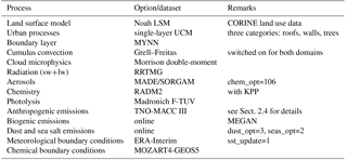
We use the Weather Research and Forecasting model (WRF) version 3.8.1 (Skamarock et al., 2008), with chemistry and aerosols (WRF-Chem, Grell et al., 2005; Fast et al., 2006). The set-up includes two model domains centred over Berlin, at horizontal resolutions of 15 km × 15 km and 3 km × 3 km, using one-way nesting. The model top is at 50 hPa, using 35 vertical levels with the first model layer top at approximately 30 m above the surface. There are 12 levels in the lowest 3 km. Urban processes (meteorology) are parameterized with the single-layer urban canopy model, with input parameters specified for Berlin as described in Kuik et al. (2016) and three urban land use categories. The set-up further includes the RADM2 chemical mechanism with the Kinetic Pre-Processor (KPP) and the MADE/SORGAM aerosol scheme. The MOZART chemical mechanism is used in a sensitivity test. All physics and chemistry schemes used in this study are listed in Table 1.
Small changes in the code have been made. The initialization of the dry deposition (module_dep_simple.F) has been adapted in order to account for three urban land use categories as described in Kuik et al. (2016), and references therein. Nighttime mixing over urban areas is not accounted for sufficiently by the urban parameterization and the PBL scheme and is thus adjusted (dry_dep_driver.F) as described in the Supplement. There, we also show illustrative results (Figs. S1–S3 in the Supplement) of two test simulations comparing the impact of changes in this model set-up with respect to Kuik et al. (2016), including the modification of nighttime mixing and the modification of the diurnal distribution of traffic emissions (see Sect. 2.4).
2.2 Model input data
We use the European Centre for Medium-Range Weather Forecasting (ECMWF) Interim reanalysis (ERA-Interim, Dee et al., 2011) with a horizontal resolution of 0.75∘ × 0.75∘ and a temporal resolution of 6 h, interpolated to 37 pressure levels (with 29 levels below 50 hPa) as meteorological initial and lateral boundary conditions. The sea surface temperature is updated every 6 h. The data are interpolated to the model grid using the standard WRF pre-processing system (WPS). Chemical boundary conditions for trace gases and particulate matter are created from simulations with global chemistry transport Model for Ozone and Related chemical Tracers (MOZART-4/GEOS-5, Emmons et al., 2010). Instead of the standard USGS land use data we use CORINE data (EEA, 2014), remapped to the USGS classes, using three categories characterizing the urban area. This provides a more realistic characterization of the land use in the Berlin–Brandenburg area (Kuik et al., 2016; Churkina et al., 2017). The emission input data and their pre-processing are described in Sect. 2.4.
2.3 Simulation procedure
Following the workflow used in AQMEII phase 2 (Brunner et al., 2015), we re-initialize the simulation every 2 days, with a 1-day spin-up of the model meteorology. To ensure consistency in the chemical fields, we start each new 2-day simulation from the chemistry fields of the previous simulation. For the base run using the RADM2 chemistry scheme, we do a full-year (2014) simulation. The results of this simulation are used to derive a correction factor for road traffic emissions, as explained in Sect. 6.1. For computational reasons, the simulation is divided into two parts covering the first 6 and last 6 months of the year. Both simulations are initialized using data from ERA-Interim (meteorology) and MOZART4/GEOS5 (chemistry) and are preceded by a spin-up period of 4 days. We do a 1-month sensitivity simulation with the MOZART chemistry scheme (July 2014), and two sensitivity simulations with increased traffic emissions for January and July 2014, all with the same simulation procedure. All model simulations are listed in Table 2.
2.4 Emissions
2.4.1 General description
The emission data used in this study are from the TNO-MACC III inventory (Kuenen et al., 2014). The latest available year is 2011, which we use for simulating the year 2014. From comparing the TNO-MACC III emissions for Germany in the years available, there was generally only a very small (decreasing) trend in reported emissions up to 2011, expected to continue also after 2011. This allows use of the latest available year of emissions (2011) also for 2014 simulations (Hugo Denier van der Gon, personal communication, 2016). Details on the emission inventory and the way these emissions are used in the present WRF-Chem set-up can be found in Kuik et al. (2016), and references therein, and are briefly summarized here. The data are originally at a horizontal resolution of ca. 7 km × 7 km, which we downscale for the Berlin–Brandenburg region based on proxy data (Fig. 1). As it has been shown that downscaling the emission data to the resolution of the model grid helps to better capture the spatial distribution of air pollutant concentrations, we updated the downscaling procedure (see Supplement). The updates include an extension of the region for which the emissions are downscaled from Berlin to the whole Berlin–Brandenburg region. In addition, we only downscale those emission categories (SNAP categories) which are both of main interest for studying NO2 in an urban area and also represented well by the proxy data chosen. This ensures that we are not suggesting a higher precision than is achievable with the available proxy data. We thus only downscale emissions from SNAP categories 2 (residential combustion), 6 (product use) and 71–75 (traffic), as these emissions can be represented well by population density (SNAP 2 and 6) and traffic density (SNAP 71–75).

Figure 1Total NOx emissions from traffic in Berlin; (a) from the TNO-MACC III inventory, 2011; (b) from the TNO-MACC III inventory, downscaled to a horizontal resolution of ca. 1 km, 2011; (c) from the Berlin Senate Department for Urban Development and Housing for the year 2009.
2.4.2 Emission processing
Kuik et al. (2016) concluded that when simulating urban air quality with high resolution and using emission input data at high resolution, a more detailed treatment of the vertical distribution of point source emissions might further improve the model results. For this reason in this study, the emissions are distributed vertically based on profiles adapted from Bieser et al. (2011), i.e. emissions from the energy industry are distributed between the third and seventh model layer, emissions from other industrial sources as well as from the extraction and distribution of fossil fuels are distributed between the first four model layers, waste treatment emissions are distributed in the first five model layers and airport emissions (LTO cycle) are distributed vertically into the first seven layers (see Supplement for further details). For reference, the layer tops are at ca. 30 m (layer 1), 95 m (layer 2), 190 m (layer 3), 310 m (layer 4), 460 m (layer 5), 650 m (layer 6) and 890 m (layer 7).
TNO-MACC III emissions are provided as annual totals. For each emission (SNAP) category separately, we apply factors distributing the emissions for each month, day of the week (weekend vs. weekday), and hour of the day (diurnal cycle) based on Builtjes et al. (2002), with the exception of the diurnal cycle of traffic emissions. Previous studies highlighted the importance of using locally available information when specifying temporal profiles of emissions (e.g. Mues et al., 2014). Here we apply a diurnal cycle of traffic emissions (fraction of total daily emissions per hour of the day) calculated based on traffic counts provided by the Berlin Senate Department for the Environment, Transport and Climate (data used from 2007 to 2016) and by the German Federal Highway Research Institute – BASt (Bundesanstalt für Straßenwesen, 2017, data used from 2003 to 2016). The diurnal cycle applied here is obtained by calculating the fraction of average daily traffic counts in Berlin at each hour of the day, thus assuming a linear scaling of traffic emissions with traffic counts as also assumed by Builtjes et al. (2002). Following Builtjes et al. (2002), we apply a uniform diurnal cycle for each day of the week, making no distinction between the diurnal cycle of weekends and weekdays. As mentioned above, we do however also apply a weekly profile; thus, the magnitude of the daily emissions on weekends is different from that on weekdays. The main differences between the profiles calculated based on locally available information and the hourly emission factors from Builtjes et al. (2002) include an earlier increase in traffic emissions in the morning by ca. 1 h and more evenly distributed high traffic emissions during the day with less pronounced morning and afternoon peaks.
NOx is emitted mainly as NO, but also includes a fraction directly emitted as NO2 (the primary NO2 fraction, f-NO2) by combustion engines. Here, NOx is emitted as NO for all SNAP categories except “road transport” and “non-road transport”. For non-road transport and all road transport emissions except diesel, NOx is emitted as 10 % NO2 and 90 % NO (by mass). Road transport diesel emissions include both light duty vehicle (LDV) and heavy duty vehicle (HDV) emissions. For the latter, we also assume a f-NO2 of 10 %, while for light duty vehicles we assume a f-NO2 of 26 % (Carslaw, 2005). Combining this with the TNO-MACC share of diesel emissions attributable to LDV (43 %) and HDV (57 %), we obtain a combined f-NO2 for road transport diesel NOx emissions (SNAP 72) of 17 %. Test simulations varying the f-NO2 for diesel LDV between 10 and 55 % have shown that the simulated NO, NO2 and NOx concentrations have very little sensitivity towards the f-NO2 of LDV diesel emissions, while small differences in the simulated ozone concentrations were seen. As further sensitivity simulations on this topic are beyond the scope of this study and differences were small, we chose to use a f-NO2 that was around the mid-point of those values documented for LDV diesel NOx emissions (26 %).
2.4.3 Comparison of the downscaled TNO-MACC III emissions with a local inventory
Local NOx emissions from road transport are available for 2009 (Berlin Senate Department for Urban Development and Housing). In comparison with the downscaled TNO-MACC III emissions for the Berlin grid cells (2011), traffic NOx emissions from the local inventory are 6 % higher. The geographical distribution of the emissions in the local inventory is very similar to the downscaled version of TNO-MACC III used in this study (Fig. 1).
3.1 AirBase observations and NO2 uncertainty
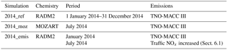
NO2, NOx and O3 measurements are taken from AirBase (EEA, 2017), a database compiling air quality observations from the EU Member States and associated countries, performed as required by EU clean air legislation. The files can directly be downloaded from the AirBase website. In the case of Germany the measurements are performed by the federal states. For the comparison with model results, observations from stations within Berlin and in the adjacent surroundings in the Federal State of Brandenburg representing “urban background”, “suburban background” and “rural near-city” conditions are used (Fig. 2; also see Supplement Fig. S4 and Table S1). For our analysis, we re-classify AirBase station DEBE066 in Berlin–Karlshorst from “urban background” to “suburban background”, as the station is not located in the core area of the city and pollutant concentrations measured there are similar to concentrations measured at other suburban background stations. As a result, four stations for each classification type are used in this study: Amrumer Straße (DEBE010), Brückenstraße (DEBE068), Belziger Straße (DEBE018) and Nansenstraße (DEBE034) in the urban background, Blankenfelde-Mahlow (DEBB086), Buch (DEBE051), Groß Glienicke (DEBB075) and Johanna und Willy Brauer Platz (DEBE066) in the suburban background, and Frohnau (DEBE062), Grunewald (DEBE032), Müggelseedamm (DEBE056) and Schichauweg (DEBE027) in the rural near-city background.
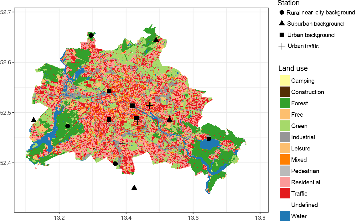
Figure 2Locations of measurement stations in and close to Berlin, including their AirBase station area classification and type and the land use classes in Berlin according to the Berlin Senate Department for Urban Development and Housing (2015).
In addition, five measurement stations representing “traffic” conditions within Berlin, which are located next to major roads within the core area of the city, and assumed to be primarily influenced by traffic emissions, are used for the observation-based analysis (Sect. 6.3).
NO2 concentrations used for this study were measured using chemiluminescence. With this method, NO2 is converted to NO with a molybdenum converter before being detected using chemiluminescence, as NO reacts with O3 to form NO2 and O2 while emitting light (see e.g. Gerboles et al., 2003; Steinbacher et al., 2007). A limitation of this method is that other nitrogen-containing species (PAN, HNO3) are also converted to NO in this process. In a comparison study, Steinbacher et al. (2007) found that only 73–82 % of the NO2 measured with this method is “real” NO2, at a rural background site in Switzerland. However, they state that reasonable results are obtained with this type of converter at urban background sites. Villena et al. (2012) compared NO2 concentrations in urban smog conditions in Santiago de Chile using chemiluminescence detection with a molybdenum converter and differential optical absorption spectroscopy and found large differences between measured concentrations during daytime. Further sources of uncertainty are introduced in the detection itself, for which NO reacts with O3, producing the luminescence signal to be detected. Gerboles et al. (2003) assess the uncertainty of NO2 measurements, and Pernigotti et al. (2013) derive a simplified procedure in order to calculate the NO2 measurement uncertainty, which we apply in order to obtain a rough estimate of the uncertainty range of NO2. Accordingly, the uncertainty (u) of the observed NO2 concentrations x at time i is quantified as follows:
Here, is an estimate of the relative uncertainty around a reference value RV, and α is the fraction of uncertainty not proportional to the reference value. We use the coefficients corresponding to the mean uncertainties of the individual parameters, i.e. .09, α=0.06 and the reference value RV = 200 µg m−3 (Pernigotti et al., 2013).
3.2 Meteorological data
In order to complement the analysis and to investigate potential influences of the modelled meteorology on modelled NO2 concentrations, we include a comparison of modelled meteorology with observations. This includes observations of 2 m temperature, and 10 m wind speed and direction, all provided by the German Weather Service and available online (Kaspar et al., 2013). In addition, mixing layer height derived from ceilometer measurements at Nansentraße during the BAERLIN2014 campaign (Geiß et al., 2017) are used for a qualitative comparison with the modelled mixing layer height (see Kuik et al., 2016, for a discussion of this type of comparison). The data are generally available between 20 June and 27 August 2014, but include a number of gaps.
4.1 Analysis of model results
Modelled NO2 concentrations are evaluated with the aim of using the model set-up for policy-relevant analyses of urban NO2 concentrations and NO2 reduction measures with high temporal and spatial resolution, and in order to identify the main sources of the errors in modelled NO2 concentrations. For this, we use both operational and diagnostic evaluation metrics, which are explained in the following.
Operational evaluation metrics applied here are based on Thunis et al. (2012) and Pernigotti et al. (2013). They include an analysis of the mean bias (MB) and normalized mean bias (NMB), the correlation coefficient (R), and the root mean square error (RMSE, as defined in the Supplement). The model error is compared with the model quality objective (MQO) and performance criteria calculated from NO2 observations and their uncertainty. The MQO is defined as follows:
with RMSU being the root mean square of the measurement uncertainty. Following Thunis et al. (2012) and Pernigotti et al. (2013), a MQO lower than 0.5 indicates that the model results are on average within the range of the measurement uncertainty, and further efforts to improve model performance are not meaningful. A MQO between 0.5 and 1 indicates that the uncertainties of model and observations overlap, and that the model might still be a better predictor of the true value than the observations. A MQO greater than 1, on the other hand, indicates significant differences between the model and the observations.
The performance criteria for mean bias, normalized mean bias and correlation coefficient as defined in Pernigotti et al. (2013) are listed in the Supplement. As the uncertainty of NO2 measurements is partly concentration-dependent, the MQO and the other performance criteria differ between station classes and seasons.
The operational evaluation and model quality objectives are intended to support an assessment of the extent to which a model can be used for policy-relevant analyses, but do not point to the underlying processes that might lead to a disagreement between model results and observations. Furthermore, the calculation of the NO2 measurement uncertainty underlying the calculation of the MQO and performance criteria is also based on a number of uncertain parameters.
We thus complement the analysis with a diagnostic evaluation, comparing the individual spectral components of the modelled and observed time series. This is done following Solazzo and Galmarini (2016) and Solazzo et al. (2017): we use a Kolmogorov–Zurbenko filter (Zurbenko, 1986), a widely used filter in the analysis of air quality data based on calculating the iterative moving average of a time series, in order to decompose the modelled and observed time series into contributions from different timescales. The Kolmogorov–Zurbenko filter is a low pass filter, with the length of the moving average window and the number of iterations determining the spectral component to be filtered. Taking the difference between two filtered time series (band-pass filter) makes it possible to decompose the observed and measured time series into an intra-diurnal component (ID, < 0.5 days), a diurnal component (DU, 0.5–2.5 days), a synoptic component (SY, 2.5–21 days) and a long-term component (LT, > 21 days) with the property
Here, TS describes the full time series of species x. This is described in detail in Solazzo et al. (2017) and Solazzo and Galmarini (2016), and references therein. Further details are also given in the Supplement.
By assessing the error of each component individually it is then easier to relate the error to the model process(es) characteristic at the respective timescale. The error analysis of the different spectral components is done by “error apportionment” (Solazzo et al., 2017), breaking down the mean square error (MSE) into bias, variance (σ) error and minimum achievable mean square error (mMSE) as follows:
As described by Solazzo and Galmarini (2016), the minimum achievable mean square error is determined by the observed variability that is not reproduced by the model. While this approach helps in investigating the sources of model errors, it does not allow for clear identification or quantification of them as several processes take place on similar timescales, and because this filtering method does not allow for a complete separation of the different spectral components (see Solazzo et al., 2017, for a discussion of this issue).
In addition to this operational and diagnostic analysis of simulated NO2 concentrations, we include a brief evaluation of selected key meteorological parameters (temperature, wind speed and direction) as well as further chemical species (O3, NOx), the former because WRF-Chem is an online-coupled model, and the latter because NO2 is tightly linked to NO and O3.
4.2 Observation-based analysis
As traffic emissions are the focus of this study, the analysis of the model results is complemented with an analysis based on observations of roadside and urban background NO2 concentrations and traffic counts. Like in many chemistry transport modelling studies, we assume a linear scaling of traffic emissions with traffic counts, which are used as a proxy for calculating time profiles of traffic emissions for each month, day of the week and hour of the day. While it has been shown that model results can be improved by taking into account country-specific driving patterns as well as by applying separate diurnal cycles for heavy and light duty vehicles (Mues et al., 2014), local traffic conditions (e.g. congestion) are currently not taken into account in the calculation of the diurnal cycles.
Using observations of traffic counts and roadside NOx concentrations in Berlin obtained at the same locations and times (data described in Sects. 2.4.2 and 3.1), we assess how much of the observed variance in NOx concentrations can be explained with traffic counts in a linear model. In addition to a linear fit, other types of relationships (e.g. quadratic, exponential) are also explored. We neglect other influences on observed NOx concentrations such as other emission sources and large-scale and local meteorological conditions. In order to account for different conditions at different hours of the day, we fit the data separately for each hour of the day. The intention of this analysis is not to build a statistical model for roadside NOx concentrations, but rather to give insight into the type of relationship between roadside NOx concentrations and traffic counts, complementing the model simulations done in this study.
5.1 Meteorology
An in-depth evaluation of modelled meteorology obtained with a similar model set-up is presented in Kuik et al. (2016) for the summer (JJA) of 2014. Here, model results for the whole year of 2014 are presented and discussed. Changes in the model set-up compared with the set-up presented in Kuik et al. (2016) are the planetary boundary layer scheme (MYNN, Nakanishi and Niino, 2006 instead of YSU, Hong et al., 2006) and re-initialization of the model meteorology every 2 days as described in Sect. 2. Tests showed that though the change in the planetary boundary layer scheme did not introduce considerable improvements, it did seem to lead to a slightly better match of model results with observations in the timing of the decrease in the boundary layer in the evening. Here an additional brief model evaluation is done in order to ensure that the modelled meteorology still reproduces observations reasonably well.
Table 3Modelled meteorology compared to observations and annual and seasonal performance indicators. Mean bias (MB) and root mean square error (RMSE) are indicated in K (temperature) and m s−1 (wind speed); the normalized mean bias (NMB) and correlation coefficient (R) are unitless. Data are aggregated as follows: MAM – March, April, May, JJA – June, July, August, SON – September, October, November, and DJF – December, January, February.
Modelled and observed 2 m temperature and 10 m wind speed are compared at five stations run by the German Weather Service, including Schönefeld, Tegel and Tempelhof in Berlin and Lindenberg and Potsdam outside of Berlin (Table 3). Across the stations, annual mean temperature is simulated well, with mean biases smaller than −1 ∘C outside of Berlin and just above −1 ∘C within Berlin. Modelled and observed hourly temperatures correlate well with R=0.96 at all five stations. Small seasonal differences exist, with somewhat higher biases in winter (as large as −1.7 ∘C in Tegel) and somewhat lower biases in spring (e.g. −0.1 ∘C in Schönefeld). Annual mean wind speed is somewhat overestimated within Berlin (between 0.02 and 0.45 m s−1, or up to 13 %), with correlations of the hourly values between 0.74 and 0.78 within Berlin. In winter, wind speed is slightly underestimated at two out of the three stations within Berlin (−2 and −7 % at Tegel and Schönefeld, respectively), while it is overestimated somewhat more in spring and summer (up to 0.58 m s−1, or ca. 20 % in Tegel). In spring and summer, the main wind directions are captured relatively well by the model (see Figs. S6 and S7 in the Supplement). In autumn, wind from the east, the main wind direction, is modelled less frequently than observed, but wind from the south-east is modelled too frequently compared with observations. In winter, modelled wind comes from south and south-west too frequently compared with observations, at the expense of south-easterly wind directions, as depicted in Figs. S6 and S7. Compared with Kuik et al. (2016), an improvement in summer mean bias in wind speed is seen; with the JJA mean bias between 0.3 and 0.4 m s−1 smaller than that of the comparable simulation in Kuik et al. (2016) at all Berlin stations, and JJA correlation coefficients improved by ca. 0.1. This can probably be attributed to the continuous re-initialization of modelled meteorology in this simulation.
In addition, modelled and ceilometer-derived mixing layer heights (MLHs) are compared (Fig. S8 in the Supplement). Even though a quantitative comparison between the modelled MLH and the MLH height derived from optical measurements is difficult to interpret (see Kuik et al., 2016), a qualitative comparison of mean diurnal cycles gives insight into the timing of the deepening of the MLH. The comparison shows that the modelled increase in the summer MLH in the morning is too early, already starting at ca. 04:00 in the model. Though the precise time of the observed MLH increase cannot be determined from the available data, it takes place between 05:00 and 07:00 (Fig. S8 in the Supplement). An early modelled deepening of the mixing layer might lead to overly early and thus overly strong mixing of chemical species in the model.
5.2 Operational evaluation of simulated chemical species
Seasonally and station-class averaged performance metrics are listed in Table 4 for NO2, NOx and O3. NO2 and total NOx are biased low throughout the seasons and station classes, with the highest (absolute and relative) mean biases for urban background stations both annually and seasonally. The model bias is relatively low at rural and suburban background stations, with annual mean biases of only up to −2.8 µg m−3 (−19 %). Correlation coefficients of modelled with observed hourly concentrations are R=0.50 and R=0.55 in the rural and suburban backgrounds, respectively.
Table 4Modelled chemistry, seasonal performance indicators (averaged for each station class; each class includes four stations) and the model quality objective for NO2. Mean bias (MB) and root mean square error (RMSE) are indicated in µg m−3; the normalized mean bias (NMB) and correlation coefficient (R) are unitless. Data are aggregated as follows: MAM – March, April, May, JJA – June, July, August, SON – September, October, November, and DJF – December, January, February.
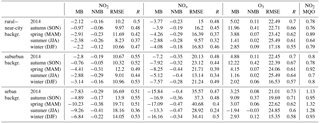
NO2 at urban background sites is biased by −7.8 µg m−3 (−29 %) on average, with a higher negative bias in spring (−10.2 µg m−3, −38 %) and summer (−9.3 µg m−3, −41 %) and smaller negative biases in autumn (−4.9 µg m−3, −17 %) and winter (−6.8 µg m−3, −22 %). Modelled hourly concentrations correlate reasonably well with observations in autumn, spring and winter (R between 0.51 and 0.55), but worse in summer (0.36).
Modelled hourly ozone concentrations correlate reasonably well with observations at all station classes throughout the whole year (R between 0.70 and 0.73), but with lower correlations for individual seasons. This shows that intra-seasonal differences are represented well by WRF-Chem, with slightly worse representations of inter-seasonal variations. Modelled ozone concentrations are biased high at most stations and in most seasons, with the exception of a low bias in summer in the urban background.
For NO2, the MQO (Eq. 2) is greater than 0.5, but smaller than 1, both annually averaged and in all seasons at rural near-city background and suburban background stations. For urban background sites the MQO is larger than 1 both on annual average and in spring and summer, and just below 1 in autumn and winter, emphasizing that the model performs reasonably well in the rural and suburban background, but the disagreement between model results and observations is larger in the urban background. This suggests that processes or emissions typical for urban areas are an important source of model error.
In order to test the sensitivity of the results to the selected chemical mechanism, we compare modelled NO2 and total NOx concentrations for July with two different chemical mechanisms: RADM2 (the base configuration in this study) and MOZART. For all station classes in and around Berlin, the modelled NOx and NO2 concentrations only show very small mean differences of −0.04 to −0.4 µg m−3 (NOx) and −0.4 to −0.5 µg m−3 (NO2, RADM2 – MOZART). This suggests that the model bias in NO2 and total NOx concentrations of the base configuration is not strongly influenced by the choice of chemical mechanism, but rather results from other sources of error.
5.3 Diagnostic evaluation of simulated NO2 concentrations
In order to further assess the model performance and identify the main sources of the model bias, a diagnostic evaluation is done, by spectrally decomposing the modelled and observed time series of NO2 and analysing the type of error of each component.
Averaging the decomposed time series over each station class, the modelled long-term (LT) and synoptic (SY) components as defined in Sect. 4.1 correlate well with the observations: the correlation coefficient for the LT component is 0.83, 0.81 and 0.72 for rural near-city, suburban and urban backgrounds, respectively, and 0.60, 0.63 and 0.65 for the SY component (Fig. 3). This suggests that changes on timescales of ca. 2.5 days to a few weeks are captured relatively well by WRF-Chem, which includes for example the modelled synoptic (meteorological) situation and is consistent with the good model performance in simulating observed meteorology. The correlation coefficients for the diurnal (DU) component are smaller, with 0.45, 0.52 and 0.48 for rural near-city, suburban and urban backgrounds, respectively. This suggests that the model has more difficulties in capturing variations on timescales of a few hours to 2.5 days than on longer timescales. This might be related to the diurnal variations in modelled mixing, but also to the diurnal cycle of emissions. Particularly the latter is strongly influenced by traffic emissions in the urban area and might also point to deviations of the model-prescribed diurnal cycle in emissions from the real-world diurnal cycle.
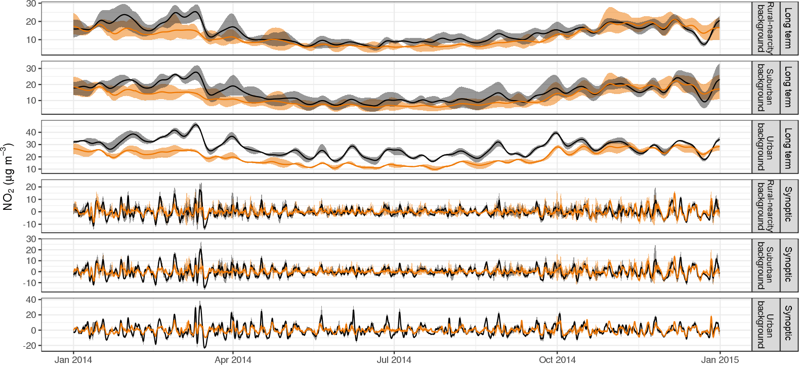
Figure 3Long-term and synoptic components of modelled (orange) and observed (black) time series, averaged over all stations of each station class. The shaded areas show the variability (25th and 75th percentiles) between the different stations within each class. Note the variable y-axis.
With the procedure used for spectrally decomposing the NO2 time series, the LT component is the only systematically biased component, with the other components fluctuating around zero. Decomposing the model error shows that the bias of the LT component has the largest contribution to the error for urban background stations (ca. 30 %, Fig. 4). NO2 has a short lifetime and is mainly influenced by local and regional sources. This means that the boundary conditions are not likely to be a strong source of error. The negative bias in the LT component is consistent with both problems in daytime vertical mixing and an underestimation of emissions. As discussed in Sect. 3.1, NO2 concentrations detected with chemiluminescence using a molybdenum converter might be biased high due to interferences with other nitrogen-containing species (e.g. PAN, HNO3) and could further contribute to discrepancies between modelled and observed NO2 concentrations.
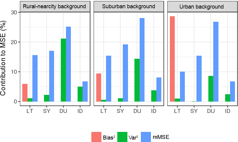
Figure 4Contribution of different types of error to the mean square error of the model, per station class. The mean square error is divided into squared bias (bias2), variance error (var2) and minimum mean square error (mMSE) of the long-term (LT), synoptic (SY), diurnal (DU) and intra-diurnal (ID) components (see Sect. 4.1 for further details).
The second largest error at urban background stations and the largest error at rural near-city and suburban background stations is the mMSE of the diurnal component. This means that part of the observed variability is not reproduced by the model and is consistent with the comparably lower correlation coefficients of the diurnal component compared with the synoptic and long-term components. Solazzo et al. (2017) relate this error to problems in comparing single point measurements with model grid cell values (incommensurability) and a disagreement in timing of modelled and observed concentrations, amongst others. The incommensurability can, in the case of NO2, come from NO2 observations being influenced by local sources that cannot be captured by WRF-Chem run at a horizontal resolution of 3 km × 3 km. The temporal variation of modelled NO2 concentrations, in the case of the diurnal component, can be influenced by the temporal profiles prescribed to the emission input data. Thus, the error is consistent with problems in the prescribed diurnal cycles of emissions including traffic emissions, but might also be related to a diurnally varying bias in emissions.
At rural near-city background stations, there is a relatively large contribution of the variance error of the diurnal component. This is probably caused by an overestimation of the standard deviation of observed diurnal components in autumn (Fig. S9 in the Supplement), particularly pronounced at the site Frohnau in the north or Berlin, slightly west of the main emission sources. This might be explained by the disagreement in modelled and observed wind direction in autumn, leading to higher than observed NO2 peaks in the model.
Solazzo et al. (2017) present a diagnostic model evaluation of the AQMEII phase 3 model simulations for the year 2010 and report the largest error of modelled NO2 in winter, both for the European and North American domains simulated in AQMEII. Our results show the opposite for urban background stations (Fig. S9 in the Supplement): the model error, and particularly the bias, is smallest in autumn and winter. While Solazzo et al. (2017) attribute the winter bias to a potential underestimation in residential combustion emissions, these seem to be captured comparably well by the TNO-MACC III inventory in the case of Berlin. The re-distribution of these emissions based on population density, as described in Sect. 2.4.2, may also have contributed to a better spatial representation in our study.
5.4 Diurnal and weekly variation of the model bias
The results from the operational and diagnostic evaluation of modelled NO2 concentrations suggest that emissions within the urban area are a main source of model error, both contributing to the model bias and the lower correlation with observations. Traffic emissions have the largest contribution to urban NOx emissions. As traffic emissions have a distinct weekly and diurnal cycle, we additionally assess mean diurnal cycles of modelled and observed NO2 concentrations as well as the differences between weekdays and weekends. This also helps to further assess the contribution of problems in modelled mixing to the model error. In addition, we analyse the MQO and performance criteria separately for weekends (Saturday and Sunday) and weekdays (Monday through Friday). Public holidays that fall on a weekday are excluded from this analysis, as they were not treated separately from regular weekdays in the emission processing.
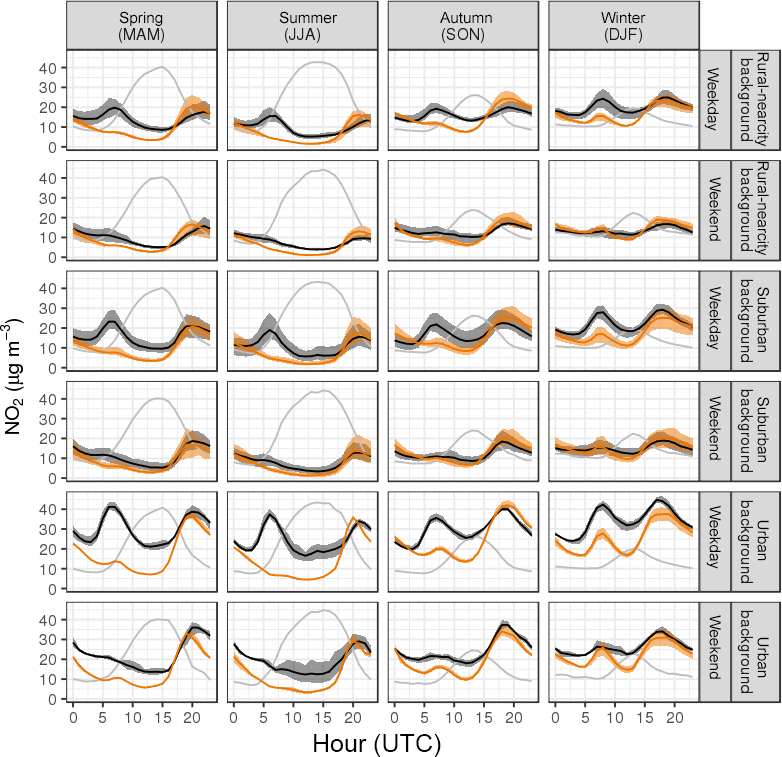
Figure 5Mean diurnal cycles of modelled (orange) and observed (black) NO2 concentrations, by station class and weekday/weekend. Shaded areas show the variability between the different stations' mean diurnal cycles (25th and 75th percentiles). Grey lines show the mean modelled planetary boundary layer heights at the respective grid points (scaled, but the relative changes between different hours and seasons are maintained).
The comparison of mean modelled and observed NO2 diurnal cycles shows distinct differences between station classes and weekend and weekday diurnal cycles (Fig. 5). The diurnal cycle of observed NO2 concentrations is modelled reasonably well for rural and suburban background stations. In particular, nighttime concentrations are simulated well for rural and suburban background stations, and mostly underestimated in the urban background. Other WRF-Chem modelling studies often report too little mixing at nighttime over urban areas leading to a strong overestimation of observed concentrations. In this study as in other modelling studies using WRF-Chem (Ravan Ahmadov, personal communication, 2017), a modification of the model code was applied in order to increase nighttime mixing. This, in combination with a more realistic vertical distribution of point source emissions (as described in Sect. 2.4.2), seems to improve model performance for NO2 during nighttime. In addition, tests revealed that this change to the model code does not impact modelled daytime concentrations.
During weekdays, there is an underestimation of the observed morning peak in all seasons and at all station classes. Weekend diurnal cycles are modelled well at rural and suburban background stations. At urban background stations there is a larger disagreement between modelled and observed concentrations throughout the whole day on both weekends and weekdays. The underestimation of daytime urban background NO2 concentrations is particularly strong in summer and spring. This might be explained by mixing over urban areas during daytime that is too strong, caused for example by a turbulent diffusion coefficient that is too large during daytime over urban areas in the lowest model layer. Other modelling studies have reported similar problems, reducing the coefficient over urban areas (e.g. of the CHIMERE model set-up used in Schaap et al., 2015). An onset of the deepening of the boundary layer that is too early (Sect. 5.1) might further contribute to the disagreement in the modelled and observed morning peaks. Overall, this discussion shows that the representation of vertical mixing over urban areas might have to be improved to be physically more consistent in regional models, for example by better taking into account urban heat and momentum fluxes and treating the urban parameterization consistently with chemistry. Measurements of vertical profiles of NOx in cities, particularly in the planetary boundary layer, would be helpful in order to evaluate the models and improve the representation of surface NOx concentrations, as the NOx profile in the lowest model layer is not resolved at the model resolution used in this study.
The model underestimation of observed daytime NO2 concentrations at urban background stations is stronger on weekdays than on weekends, and is particularly noticeable during the morning hours. This is consistent with an overall underestimation of emission sources active in the morning hours on weekdays and potentially also a misrepresentation of the diurnal cycles of emissions in the model: traffic emissions are distributed in the model throughout the day using a linear scaling with traffic counts (Sect. 2.4.2), which might fall short of accounting for relatively higher emissions during situations with high traffic and associated congestion. This issue is further assessed in Sect. 4.2.
Generally, throughout all seasons, the NO2 MQO is not met on weekdays for urban background stations, but is smaller than 1 on weekends (Fig. 6). The patterns of the model–observation disagreement, and particularly the weekend–weekday differences, are consistent with traffic emissions as a main source of the bias, with a particularly large contribution to observed urban background concentrations.
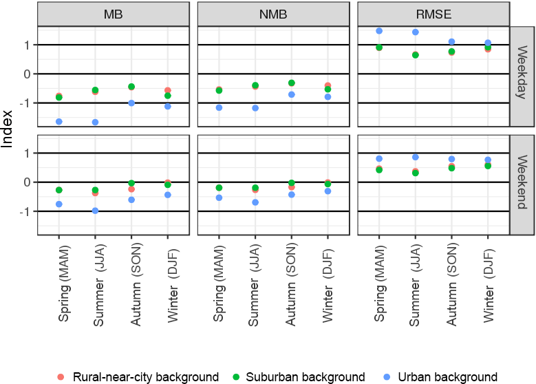
Figure 6Skill of WRF-Chem in simulating daytime (06:00–17:00 UTC) observed NO2 concentrations. The index represents the the model quality objective for the root mean square error (Sect. 4.1) and the performance criteria for mean and normalized mean bias (described in the Supplement), for weekend and weekday days and each month/season.
6.1 Calculation of a correction factor
The results from the operational and diagnostic evaluation of modelled NO2 concentrations suggest that traffic emissions are a main source of model error in the urban background: the bias and the mMSE of the diurnal component have the largest contribution to the model error in the urban background throughout all seasons, which is consistent with both an underestimation of the magnitude of traffic emissions, and a problem with their temporal distribution. This is further supported by the smaller (absolute and relative) daytime bias of modelled NO2 concentrations on weekends, where there is less traffic. In the following, we derive a correction factor based on this model bias, which represents the degree to which traffic emissions are underestimated in Berlin, but also takes into account that other sources of model error are likely to also contribute to this bias.
Besides biases in traffic emissions, problems in modelled mixing, which is particularly relevant in summer and spring when the mixed layer is deeper than in other seasons, might contribute to the model bias. Other contributions to the NO2 bias might come from deviations of modelled from observed wind speed in certain periods, and a potential overestimation of NO2 in the observations by detection of other nitrogen-containing compounds as discussed above. These sources of error are likely to impact the model results equally on both weekends and weekdays, whereas an underestimation of traffic emissions will have the largest impact on the results on weekdays. For the quantification of the underestimation of traffic emissions we assume that the weekend bias is entirely caused by non-traffic-emission-related sources of error and thus use the difference between weekday and weekend bias as an estimate for the traffic-related bias. We use the weekday–weekend difference of the relative biases (Fig. 7), thus assuming that the model error due to other sources than traffic emissions roughly scales with the magnitude of modelled concentrations. These are both conservative assumptions, as the correction factor would be much larger if the whole weekday bias was regarded as caused by traffic emissions, and it would also be larger if the absolute weekday–weekend difference was used.
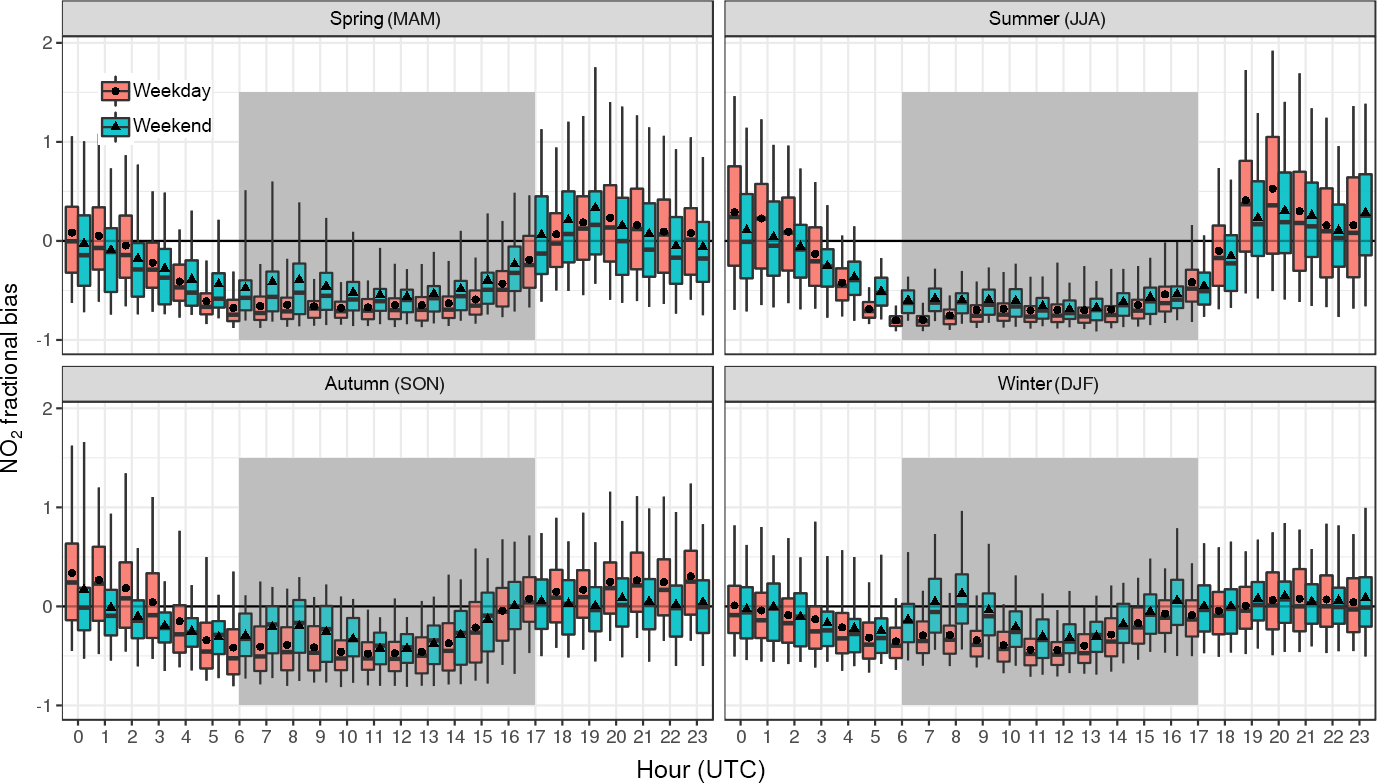
Figure 7Relative bias in modelled NO2 concentrations at urban background sites in Berlin, averaged over each season, hour and weekend/weekday. The boxplot shows median (line), 25th and 75th (box), and 5th and 95th (whiskers) percentiles of the hourly bias. Points show the mean. The grey shaded area shows the time period considered for quantifying the underestimation of daytime traffic emissions.
In order to estimate the correction factor for traffic NOx emissions, we combine the weekday increment of the model bias as defined above with the average fraction of NOx emissions from traffic to total NOx emissions in Berlin. The nighttime model bias on weekends and weekdays at urban background stations is of similar magnitude on weekends and weekdays (Fig. 5). A t-test shows that the differences between weekday and weekend bias are not statistically significant at a 95 % confidence interval after ca. 17:00 UTC and before ca. 05:00 UTC (depending on the season). Furthermore, traffic emissions used in the model contribute only little to the total NOx emissions before 06:00 UTC. This suggests that an underestimation of traffic emissions is only likely to have a significant contribution to the bias in modelled NO2 concentrations between ca. 06:00 and 17:00 UTC. Within the core area of the city where traffic is high (all areas within the “S-Bahn ring”/main core of the city), the average contribution of traffic NOx to total NOx between 06:00 and 17:00 UTC is between ca. 30 and 55 %, depending on the month and hour of the day. Seasonal average values over the indicated time period are used for the calculation of the correction factor, with 37 % in winter, 47 % in summer and 42 % in autumn and spring.
With the above assumptions, we quantify the underestimation of traffic NOx emissions in the core urban area on weekdays between 06:00 and 17:00 UTC as follows, calculating a correction factor :
With the (negative) NMB = , and st denoting the traffic share of NOx emissions. Averaged over all urban background stations, and all seasons, as well as the time period between 06:00 and 17:00 this results in a correction factor of ca. 3. When averaged over all hours of the day, this factor corresponds to an overall underestimation of NOx traffic emissions in the urban centre by a factor of ca. 2, and an underestimation of all-source NOx emissions in the urban centre by a factor of ca. 1.5.
In order to gain more insight into the underestimation of the NOx emissions, we calculate a separate correction factor for each hour and season based on hourly mean seasonal biases and traffic NOx emission shares (Fig. S10 in the Supplement). The seasonal correction factors show a small increase between 06:00 and 08:00 with a subsequent decrease, and then remain relatively constant from 11:00 to 17:00. The diurnal variations of the factors for the different seasons are qualitatively similar, and the factors vary in magnitude within a range of ca. 1 between the seasons, with the factors being larger in winter than in summer. The diurnal cycle of the correction factor could be due to a diurnally varying importance of other sources of the modelled NO2 bias than the traffic emissions, such as mixing, but might also be due to a disagreement in the prescribed diurnal cycle of traffic emissions with the real-world diurnal cycle of traffic emissions. The seasonal differences can at least partly be explained with the seasonally varying relevance of other sources of model error, such as mixing, which has a bigger impact in summer and thus also leads to a bigger bias on the weekends, reducing the weekday increment. The seasonal differences might also be influenced by the temperature dependence of NOx emissions in newer diesel cars (Hausberger and Matzer, 2017), leading to higher NOx emissions at colder temperatures, which are not captured by the model.
Overall, the assumptions in these calculations are rather conservative: assuming the weekend bias is not caused by an underestimation of traffic emissions at all is likely to underestimate the effect of any traffic bias. As mentioned above, using the absolute weekday increment of the bias would also lead to higher correction factors. A further discussion of the model bias and correction factor looking into potential reasons contributing to an underestimation of traffic NOx emissions is presented in Sect. 6.4.
6.2 Sensitivity simulation with increased emissions
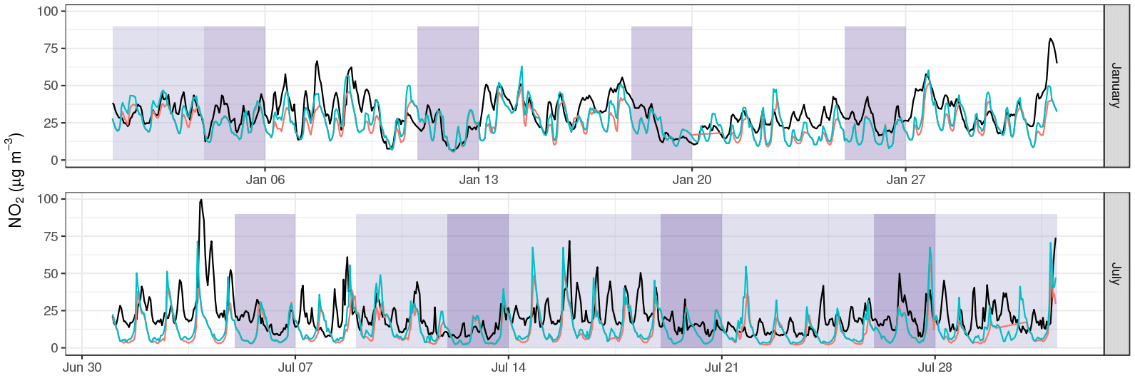
Figure 8Time series of hourly observed (black line) and modelled NO2, comparing the base simulation (red) with the sensitivity simulations (blue) using increased traffic emissions by a factor of 3 between 06:00 and 17:00 UTC on weekdays. The time series are averaged over all 4 urban background stations. Weekends are highlighted in dark purple, and holidays are highlighted in light purple.
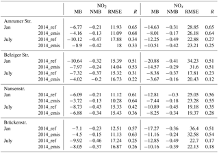
Table 5Statistics of modelled NO2 and NOx concentrations for January and July, for the base simulation and for the sensitivity simulation with increased traffic emissions, at the urban background stations in Berlin. Mean bias (MB) and root mean square error (RMSE) are indicated in µg m−3, the normalized mean bias (NMB) and correlation coefficient (R) are unitless.
The weekday correction factor was applied to NOx traffic emissions for the core urban area of Berlin (within the “S-Bahn Ring”) and tested in two sensitivity simulations for January and July 2014. The results (Table 5 and Fig. 8) show that the bias of modelled NO2 concentrations at urban background stations decreases on average by 2.6 µg m−3 (NMB decreases from −24 to −16 %) in January, and by 2.0 µg m−3 (from −43 to −34 %) in July when applying the correction factors for NOx emissions from traffic. The decrease is larger when only considering weekdays, with a mean bias lower by 3.4 µg m−3 (from −26 to −16 %) in January and by 2.7 µg m−3 (from −46 to −34 %) in July. NO2 concentrations on weekends are still represented reasonably well by the model in January (Fig. 8). The weekend bias is only changed (decreased) by lower than 0.4 µg m−3 in both cases. Only a minor change would be expected, since emissions on the weekend are not changed in the sensitivity simulations, compared to the base simulation. In January, the correlation of modelled with observed NO2 concentrations in the urban background is improved by between 0.03 and 0.06 for urban background stations in the sensitivity simulation, but this is not the case in July (Table 5). The lack of improvement in the July correlation coefficient could be related to nighttime concentrations in July that seem to be very sensitive to the increase in emissions during daytime (Fig. 8, lower panel). Despite an improved representation of nighttime concentrations compared to a previous study (Kuik et al., 2016), this sensitivity suggests the need for further attention to mixing processes in urban areas in high-resolution chemistry transport models.
Bigger improvements are seen when comparing total NOx: the mean bias for urban background stations is reduced from −16.4 to −10.3 µg m−3 (NMB decreased from −35 to −22 %) in January and from −11.1 to −8.1 µg m−3 (from −45 to −33 %) in July. Only considering weekday concentrations, these are improved by 8.1 and 3.9 µg m−3 (from −37 to −12 and −48 to −33 %) in January and July, respectively. The differences in NO2 and NOx improvements suggest that the impact of the primary NO2 fraction in emitted NOx on modelled NO2 and NOx concentrations, as well as the influence of chemical processes such as NO titration and other relevant physical and chemical processes, might need to be assessed in greater detail.
While on average the normalized mean bias in a modelled rural and suburban background is only reduced by 1–2 % in both January and July, the simulation of NO2 and NOx concentrations downwind of the city centre is improved considerably in the sensitivity simulation. To analyse the change in modelled downwind concentrations, the results are broadly divided based on four main wind directions (N, W, S, E). For each wind direction bin, the results of two stations outside the core urban area are analysed, with Frohnau and Buch in the north, Johanna und Willi Brauer Platz and Mueggelseedamm in the east, Schichauweg and Blankenfelde-Mahlow in the south and Gross Glienicke and Grunewald in the west. Only situations with wind speeds above 2 m s−1 are considered. The statistics are calculated for stations where at least 72 hourly model–observation pairs exist in the respective wind direction bin, leaving four stations in January and six stations in July for the analysis, with between 91 and 228 model–observation pairs. With some differences between the stations, the bias of weekday downwind NO2 concentrations was reduced by between ca. 1.5 and 2.9 µg m−3 January and ca. 0.4 and 1.5 µg m−3 in July. Thus, downwind NO2 concentrations in the sensitivity simulation are only biased by ca. −4 % (January) and −14 % (July) on average (as compared to −12 and −22 % in the base run). This shows that the increase in traffic emissions also helps improve modelled downwind concentrations.
Overall, in both January and July, the bias in modelled urban background NO2 and NOx is improved but still negative. Modelled downwind NO2 concentrations are improved considerably, but with low negative biases remaining also in this case. The improvements are consistent with an underestimation of traffic emissions being a main source of error. However, the results also suggest that on the one side traffic emissions might still be too low, which is consistent with the correction factor being a rather conservative estimate. On the other side, a still negative bias is also consistent with other sources of error contributing considerably to the model–observation differences as discussed previously. A relatively large bias in July remains, consistent with the mixing being an additional main source of error, particularly in summer.
Modelled O3 concentrations are not very sensitive to the changes in NOx concentrations. On average, modelled O3 is reduced at urban background stations in January by 1.5 µg m−3 (NMB decreases from 29 to 22 %). In July, the increased NOx leads to a reduction in the already negatively biased O3 from the model, with the mean bias changing from −7.3 to −8.6 µg m−3 (−11 to −13 %). Similarly, simulated O3 concentrations downwind of the city (in analogue to the downwind NO2 concentrations described above) are biased negatively in both the base run and sensitivity study in July. The bias of downwind concentrations changes from −5.4 µg m−3 (−7 %) in the base run to −6.8 µg m−3 (−9 %) in the sensitivity run. The negative bias in both NOx and O3 in the base run is consistent with the model simulating insufficient NOx emissions in a NOx-limited ozone production regime. The reduction of O3 concentrations in response to increased NOx emissions is however consistent with the model actually being in a NOx-saturated (VOC-limited) ozone production regime. The representation of VOC emissions in the model could play a role in explaining this discrepancy, as for example biogenic VOC emissions in the Berlin–Brandenburg urban area are underestimated when using WRF-Chem and MEGAN (Churkina et al., 2017). A comprehensive analysis of the simulated ozone production regime is beyond the scope of this work.
6.3 Analysis based on traffic counts
The model bias and the calculated correction factors show a diurnal cycle, with a larger model bias/correction factor in the morning hours. As explained in Sect. 5.3 and 5.4, one reason for this might be differences between prescribed and real-world diurnal cycles of the emissions. The diurnal cycle of traffic emissions in the model is calculated based on traffic counts for Berlin, assuming a linear scaling of traffic emissions with traffic counts, as done in many modelling studies.
Here, we use 3 years of hourly observations of roadside NOx concentrations and traffic counts measured at the same stations in order to get insights into the relationship between NOx concentrations and traffic counts. A linear regression model does not explain the variance of observed NOx concentrations at nighttime, as indicated by the R2 close to 0 in Fig. 9. However, during daytime, traffic counts alone explain up to ca. 40 % of observed NOx variance, particularly during the traffic rush hours. The explained variance is smaller during the afternoon peak. In comparison to a linear relationship, a quadratic relationship (NOx ∝ (traffic_count)2) does not explain more of the observed variance (not shown). An exponential relationship (NOx ∝ exp(traffic_count)), however, does explain a considerably larger share of the observed variance during daytime and particularly during the traffic rush hours, as depicted in Fig. 9 (up to ca. 60 % depending on the station).
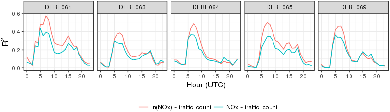
Figure 9Comparison of R2 for linear and exponential fits of roadside NOx concentrations with traffic counts.
This simple comparison suggests that roadside NOx concentrations, and thus most likely also road transport NOx emissions, scale more than linearly with traffic counts at times when the traffic intensity is high and underline that the assumption of a linear scaling of traffic emissions with traffic counts does not reflect the diurnal variation of traffic emissions sufficiently. More highly congested roads are typical in the morning, and emission factors (e.g. from HBEFA) are higher in congested situations compared to free-flowing traffic. Differences in congestion could contribute to explaining the non-linear scaling of NOx concentrations with traffic intensity. While the impact might not be large when simulating air quality with coarser models, it might play a more important role in high-resolution air quality modelling, and the temporal distribution of emissions could potentially be improved when taking these differences into account.
6.4 Discussion of traffic emissions
Based on a comparison of modelled and observed NO2 concentrations, we estimate that traffic emissions in the urban core of Berlin are underestimated by a factor of ca. 3 on weekdays between ca. 06:00 and 17:00 UTC. This corresponds to an overall underestimation of NOx traffic emissions (all-day average) in the urban centre by a factor of ca. 2, and an underestimation of total NOx emissions (all-day average) in the urban centre by a factor of ca. 1.5. Reasons for the underestimation of emissions used in this study can include limitations in the applicability of the emission inventory used here for high-resolution urban air quality modelling, problems in the temporal distribution of emissions, but also a general underestimation of traffic NOx emissions in the inventories. These three points are discussed further in the following.
First, while a reasonably good model performance can be achieved using the downscaled version of the TNO-MACC III inventory outside of the urban areas, the deviations of modelled from observed NO2 in the urban background might point to limitations in the applicability of these types of emission inventories for high-resolution modelling of NO2 in urban areas. The horizontal resolution of the original TNO-MACC III emission data is ca. 7 km × 7 km and national totals are disaggregated on the grid based on traffic intensities. Spatial differences in congestion, with emissions greatly varying between the different driving conditions and with car speed (e.g. Hausberger and Matzer, 2017), are probably not well resolved. A comparison of the downscaled version of the TNO-MACC III inventory for Berlin with a local inventory has, however, not revealed major differences in road transport emissions (see Sect. 2.4.3), suggesting that a static highly resolved local inventory based on detailed local information is not likely to improve the model results by much.
Second, in addition to spatially unresolved differences in driving conditions and related emission factors locally increasing the underestimation of emissions, the diurnal cycle of the bias in all seasons suggest that the diurnal cycle of traffic emissions also does not sufficiently account for temporal differences in driving conditions. This is consistent with the observation-based analysis, suggesting that observed NOx concentrations do not scale linearly with traffic counts. While these assumptions might be valid for coarser model resolutions, they may need to be revisited when going to higher resolutions with a focus on urban areas. However, modelled NO2 concentrations are broadly underestimated throughout the day, which means that deviations of the model diurnal cycle from the real-world diurnal cycle alone cannot explain the underestimation of modelled NO2 and NOx concentrations.
Third, traffic NOx emissions may be underestimated generally by emission inventories. The correction factor calculated here is in line with the results from other studies quantifying traffic emission underestimations in Europe, reporting traffic NOx underestimations of around 80 % (Lee et al., 2015), a factor of 1.5–2 (Lee et al., 2015) and up to a factor of 4 (Karl et al., 2017). A potential reason for the underestimation in NOx emissions from traffic can be discrepancies between real-world emission factors and those used in emission inventories. Even though HBEFA emission factors, which are often used for calculating emissions, are based on real-world driving conditions, the latest update of the handbook reports higher emission factors than previously assumed for Euro 6 and Euro 4 diesel cars (Hausberger and Matzer, 2017), e.g. an increase by ca. 50 % in case of Euro 6 vehicles (Fig. 14 in Hausberger and Matzer, 2017). In addition, the update assesses the temperature dependence of emission factors and concludes that it may lead to increases in NOx emissions of more than 30 %, compared with standard test conditions. NOx emissions from diesel cars increase with decreasing temperatures (Hausberger and Matzer, 2017). This may also contribute to the larger correction factor calculated for the winter months. Finally, while some amount of congestion is included/assumed in the emission inventories, this might be an aspect that is underestimated in terms of severity and extent.
The first and second points of this discussion suggest that improvements might be achieved by combining high-resolution chemical transport models with more detailed approaches of calculating emissions. Coupling with a traffic model, for example, might allow for not only being able to take local differences in traffic conditions into account, but also prescribe a more realistic diurnal cycle of traffic emissions. Dispersion modelling and street canyon modelling (e.g. OSPM, Berkowicz, 2000) often already take a more detailed calculation of traffic emissions into account, and different emission modelling approaches exist (e.g. traffic models such as MATSim, Horni et al., 2016). The benefit of high-resolution chemistry transport modelling, e.g. their ability to assess the impact of different emission sources on air quality on larger scales and downwind of the main emission sources, could be further exploited if coupled with existing, more detailed approaches in calculating traffic emissions or general improvements in the accuracy and resolution of emission inventories.
The consistent findings that inventories of European traffic emissions may be underestimated, coming from studies using very different methodologies, suggest that further research is necessary in order to understand real-world traffic emissions and to represent them in the inventories accordingly. Alternative measurement approaches could help verify the assumptions underlying the calculation of emissions, and help identify potential systematic problems.
Several modelling studies, particularly for Europe, have reported an underestimation of modelled NO2 concentrations compared with observations. Measurement studies also suggest that there might be considerable differences between measured urban NOx emissions and emissions provided by emission inventories based on official reporting, particularly when the contribution of traffic is large. This study quantifies the underestimation of traffic NOx emissions using WRF-Chem in a top–down approach, with the Berlin–Brandenburg area in Germany as a case study. The emission inventory used here is TNO-MACC III, downscaled to 1 km × 1 km over the Berlin–Brandenburg area based on local proxy data. The downscaled traffic emissions averaged over Berlin only differ by 6 % from a local bottom–up traffic emission inventory.
A diagnostic evaluation of the model results shows that particularly in the rural and suburban background, the long-term and synoptic components representing processes at timescales of the order of 2.5 to 21 (synoptic) and longer than 21 days (long-term) are simulated well by the model. This suggests that the modelled impact of meteorology on concentrations is represented well overall. The largest contribution to the model error comes from the (negative) bias in the urban background, and from deviations of modelled from observed variability of the diurnal component (0.2–2.5 days). This suggests a possible underestimation of urban emissions, of which traffic is the single most important contributor to NOx emissions, but is also consistent with deficiencies in other processes varying on the diurnal scale such as the modelled mixing in the planetary boundary layer. The analysis of the model results suggests that the latter is particularly relevant in summer and spring, and that further research is needed in order to better represent urban processes and their coupling with chemistry in WRF-Chem. For example, the changes in the model code applied here to improve nighttime mixing can be critically discussed, and would ideally be replaced by an improved parameterization of urban processes. The latter would need to better account for urban heat and momentum fluxes for a more realistic representation of mixing both at daytime and at nighttime, particularly in summer. An alternative model configuration to be tested could be the recently extended ACM2 planetary boundary parameterization (Pleim, 2007), which now conducts mixing of chemical species within the planetary boundary layer scheme. In addition, measurements of vertical profiles of NOx in urban areas are needed to evaluate and improve models for applications in urban areas.
The analysis of the diurnal cycle of the model bias as well as a simple observation-based calculation showing that roadside NOx concentrations scale non-linearly with traffic counts suggest that a further source of error is likely the prescribed diurnal cycle used for traffic emissions. In this study as well as in many other modelling studies, the diurnal cycle of traffic emissions is calculated assuming a linear scaling of traffic emissions with traffic counts. While this might be sufficient for coarser model resolutions, high-resolution urban air quality modelling with chemistry transport models might benefit from a more detailed temporal distribution, not only taking into account traffic intensity via a scaling with traffic counts, but also diurnal differences in congestion.
We quantify the underestimation of traffic emissions based on the finding that the weekday bias in modelled NO2 is larger than on weekends and that the contribution of traffic NOx to total NOx emissions in the urban area is typically higher on weekdays. The results suggest that traffic emissions are underestimated by ca. a factor of 3 in the core urban area on weekdays when traffic is highest (06:00 to 17:00 UTC). The underlying assumption is that other sources of model errors influence the model bias equally on weekdays and weekends, with the underestimation of traffic emissions having the largest effect on modelled NO2 concentrations on weekdays. This underestimation corresponds to an underestimation of weekly mean traffic NOx emissions in the core urban area of ca. a factor of ca. 2 and an underestimation of total NOx emissions in the city centre by a factor of ca. 1.5. Two sensitivity simulations for January and July 2014 with NOx emissions from traffic scaled with the estimated correction factor show that increased traffic emissions improve the model bias in NO2 and NOx concentrations in both seasons in the urban background, and also improve modelled downwind concentrations. The still negative bias is consistent with the factor being a rather conservative estimate.
The emission inventory used in this study is based on officially reported emissions by the individual countries, and the emissions are spatially distributed by TNO based on proxy data. Assuming the quality and accuracy of the proxy data are similar at least for larger German cities, and considering that modelling studies for other German cities have also shown an underestimation of simulated NO2 concentrations using the same emission inventory, we would assume that the results found in this study for Berlin may generally be transferrable to at least other German metropolitan areas. The underestimation of NO2 concentrations throughout the day, the consistency of the calculated correction factor with findings from other studies and the improvement of model results applying the correction factor suggest that more research is needed in order to more accurately understand the spatial and temporal variability in real-world NOx emissions from traffic, and apply this understanding to the inventories used in high-resolution chemical transport models. Given the above considerations, this not only holds for the urban area of Berlin, but for German and most likely European metropolitan areas more generally.
WRF-Chem is an open-source, publicly available community model. A new, improved version is released approximately twice a year. The WRF-Chem code is available at http://www2.mmm.ucar.edu/wrf/users/download/get_source.html (last access: 8 June 2018; Skamarock et al., 2008). The corresponding author will provide the modifications introduced and described in Sect. 2.1 upon request.
The observational and model input data used in this study are publicly available (references indicated in the paper) or available upon request.
The supplement related to this article is available online at: https://doi.org/10.5194/acp-18-8203-2018-supplement.
The authors declare that they have no conflict of interest.
This work was hosted by IASS Potsdam, with financial support provided by the
Federal Ministry of Education and Research of Germany (fBMBF) and the
Ministry for Science, Research and Culture of the State of Brandenburg
(MWFK). The authors would like to thank Hugo Denier van der Gon and Jeroen
Kuenen (TNO) for providing data of and information pertaining to the TNO-MACC
III inventory and cooperation on the downscaling of the data to a higher
resolution; Klaus Schäfer (KIT) for ceilometer data; and Mark Lawrence
(IASS), Martijn Schaap (TNO), Ravan Ahmadov (NOAA), Joana Leitao (IASS),
Stefano Galmarini (JRC) and Betsy Weatherhead (NCAR) for discussions that
helped shape the manuscript.
Edited by: Robert
Harley
Reviewed by: three anonymous referees
Berkowicz, R.: OSPM – a parameterised street pollution model, in: Urban Air Quality: Measurement, Modelling and Management, Springer, 323–331, https://doi.org/10.1007/978-94-010-0932-4_35, 2000. a
Berlin Senate Department for Urban Development and Housing: Environment Atlas Berlin, available at: http://www.stadtentwicklung.berlin.de/umwelt/umweltatlas/ed312_01.htm, last access: December 2015. a
Bessagnet, B., Pirovano, G., Mircea, M., Cuvelier, C., Aulinger, A., Calori, G., Ciarelli, G., Manders, A., Stern, R., Tsyro, S., García Vivanco, M., Thunis, P., Pay, M.-T., Colette, A., Couvidat, F., Meleux, F., Rouïl, L., Ung, A., Aksoyoglu, S., Baldasano, J. M., Bieser, J., Briganti, G., Cappelletti, A., D'Isidoro, M., Finardi, S., Kranenburg, R., Silibello, C., Carnevale, C., Aas, W., Dupont, J.-C., Fagerli, H., Gonzalez, L., Menut, L., Prévôt, A. S. H., Roberts, P., and White, L.: Presentation of the EURODELTA III intercomparison exercise – evaluation of the chemistry transport models' performance on criteria pollutants and joint analysis with meteorology, Atmos. Chem. Phys., 16, 12667–12701, https://doi.org/10.5194/acp-16-12667-2016, 2016. a, b
Bieser, J., Aulinger, A., Matthias, V., Quante, M., and Van Der Gon, H. D.: Vertical emission profiles for Europe based on plume rise calculations, Environ. Pollut., 159, 2935–2946, https://doi.org/10.1016/j.envpol.2011.04.030, 2011. a
Brunner, D., Savage, N., Jorba, O., Eder, B., Giordano, L., Badia, A., Balzarini, A., Baró, R., Bianconi, R., Chemel, C., Curci, G., Forkel, R., Jiménez-Guerrero, P., Hirtl, M., Hodzic, A., Honzak, L., Im, U., Knote, C., Makar, P., Manders-Groot, A., Meijgaard, E. V., Neal, L., Pérez, J. L., Pirovano, G., Jose, R. S., Schröder, W., Sokhi, R. S., Syrakov, D., Torian, A., Tuccella, P., Werhahn, J., Wolke, R., Yahya, K., Zabkar, R., Zhang, Y., Hogrefe, C., and Galmarini, S.: Comparative analysis of meteorological performance of coupled chemistry-meteorology models in the context of AQMEII phase 2, Atmos. Environ., 115, 470–498, https://doi.org/10.1016/j.atmosenv.2014.12.032, 2015. a
Builtjes, P., Loon, M. V., Schaap, M., Teeuwisse, S., Visschedijk, A., and Bloos, J.: The development of an emission data base over Europe and further contributions of TNO-MEP, available at: https://www.umweltbundesamt.de/sites/default/files/medien/publikation/long/3607.pdf (last access: 4 June 2018), 2002. a, b, c, d
Bundesanstalt für Straßenwesen: available at: http://www.bast.de/DE/Verkehrstechnik/Fachthemen/v2-verkehrszaehlung/Stundenwerte.html?nn=626916 (last access: 4 June 2018), 2017. a
Carslaw, D. C.: Evidence of an increasing NO2/NOX emissions ratio from road traffic emissions, Atmos. Environ., 39, 4793–4802, https://doi.org/10.1016/j.atmosenv.2005.06.023, 2005. a
Churkina, G., Kuik, F., Bonn, B., Lauer, A., Grote, R., Tomiak, K., and Butler, T. M.: Effect of VOC Emissions from Vegetation on Air Quality in Berlin during a Heatwave, Environ. Sci. Technol., 51, 6120–6130, https://doi.org/10.1021/acs.est.6b06514, 2017. a, b
Dee, D. P., Uppala, S. M., Simmons, A. J., Berrisford, P., Poli, P., Kobayashi, S., Andrae, U., Balmaseda, M. A., Balsamo, G., Bauer, P., Bechtold, P., Beljaars, A. C. M., Van De Berg, L., Bidlot, J., Bormann, N., Delsol, C., Dragani, R., Fuentes, M., Geer, A. J., Haimberger, L., Healy, S. B., Hersbach, H., Hólm, E. V., Isaksen, L., Kållberg, P., Köhler, M., Matricardi, M., Mcnally, A. P., Monge-Sanz, B. M., Morcrette, J.-J., Park, B.-K., Peubey, C., De Rosnay, P., Tavolato, C., Thépaut, J.-N., and Vitart, F.: The ERA-Interim reanalysis: configuration and performance of the data assimilation system, Q. J. Roy. Meteor. Soc., 137, 553–597, https://doi.org/10.1002/qj.828, 2011. a
Degraeuwe, B., Thunis, P., Clappier, A., Weiss, M., Lefebvre, W., Janssen, S., and Vranckx, S.: Impact of passenger car NOx emissions and NO2 fractions on urban NO2 pollution – Scenario analysis for the city of Antwerp, Belgium, Atmos. Environ., 126, 218–224, https://doi.org/10.1016/j.atmosenv.2015.11.042, 2016. a, b
Dennis, R., Fox, T., Fuentes, M., Gilliland, A., Hanna, S., Hogrefe, C., Irwin, J., Rao, S. T., Scheffe, R., Schere, K., Steyn, D., and Venkatram, A.: A framework for evaluating regional-scale numerical photochemical modeling systems, Environ. Fluid Mech., 10, 471–489, https://doi.org/10.1007/s10652-009-9163-2, 2010. a
EEA: EMEP/EEA air pollutant emission inventory guidebook 2013 – Technical guidance to prepare national emission inventories, available at: https://www.eea.europa.eu/publications/emep-eea-guidebook-2013 (last access: 4 June 2018), European Environment Agency, Copenhagen, Denmark, 2013. a
EEA: CORINE land cover data 2006, updated, available at: http://www.eea.europa.eu/data-and-maps/data/corine-land-cover-2006-raster-3 (last access: 4 June 2018), European Environment Agency, Copenhagen, Denmark, 2014. a
EEA: Air quality in Europe – 2016 report, https://doi.org/10.2800/80982, available at: https://www.eea.europa.eu/publications/air-quality-in-europe-2016 (last access: 4 June 2018), 2016. a, b, c, d, e, f
EEA: AirBase – The European air quality database, available at: https://www.eea.europa.eu/data-and-maps/data/airbase-the-european-air-quality-database-8 (last access: 4 June 2018), 2017. a
Emmons, L. K., Walters, S., Hess, P. G., Lamarque, J.-F., Pfister, G. G., Fillmore, D., Granier, C., Guenther, A., Kinnison, D., Laepple, T., Orlando, J., Tie, X., Tyndall, G., Wiedinmyer, C., Baughcum, S. L., and Kloster, S.: Description and evaluation of the Model for Ozone and Related chemical Tracers, version 4 (MOZART-4), Geosci. Model Dev., 3, 43–67, https://doi.org/10.5194/gmd-3-43-2010, 2010. a
Fallmann, J., Forkel, R., and Emeis, S.: Secondary effects of urban heat island mitigation measures on air quality, Atmos. Environ., 125, 199–211, https://doi.org/10.1016/j.atmosenv.2015.10.094, 2016. a
Fast, J. D., Gustafson, W. I., Easter, R. C., Zaveri, R. A., Barnard, J. C., Chapman, E. G., Grell, G. A., and Peckham, S. E.: Evolution of ozone, particulates, and aerosol direct radiative forcing in the vicinity of Houston using a fully coupled meteorology-chemistry-aerosol model, J. Geophys. Res.-Atmos., 111, d21305, https://doi.org/10.1029/2005JD006721, 2006. a
Geiß, A., Wiegner, M., Bonn, B., Schäfer, K., Forkel, R., von Schneidemesser, E., Münkel, C., Chan, K. L., and Nothard, R.: Mixing layer height as an indicator for urban air quality?, Atmos. Meas. Tech., 10, 2969–2988, https://doi.org/10.5194/amt-10-2969-2017, 2017. a
Gerboles, M., Lagler, F., Rembges, D., and Brun, C.: Assessment of uncertainty of NO2 measurements by the chemiluminescence method and discussion of the quality objective of the NO2 European Directive, J. Environ. Monitor., 5, 529–540, https://doi.org/10.1039/b302358c, 2003. a, b
Giordano, L., Brunner, D., Flemming, J., Hogrefe, C., Im, U., Bianconi, R., Badia, A., Balzarini, A., Baró, R., Chemel, C., Curci, G., Forkel, R., Jiménez-Guerrero, P., Hirtl, M., Hodzic, A., Honzak, L., Jorba, O., Knote, C., Kuenen, J., Makar, P., Manders-Groot, A., Neal, L., Pérez, J., Pirovano, G., Pouliot, G., José, R. S., Savage, N., Schröder, W., Sokhi, R., Syrakov, D., Torian, A., Tuccella, P., Werhahn, J., Wolke, R., Yahya, K., Žabkar, R., Zhang, Y., and Galmarini, S.: Assessment of the MACC reanalysis and its influence as chemical boundary conditions for regional air quality modeling in AQMEII-2, Atmos. Environ., 115, 371–388, https://doi.org/10.1016/j.atmosenv.2015.02.034, 2015. a
Grell, G. and Baklanov, A.: Integrated modeling for forecasting weather and air quality: A call for fully coupled approaches, Atmos. Environ., 45, 6845–6851, https://doi.org/10.1016/j.atmosenv.2011.01.017, 2011. a
Grell, G. A., Peckham, S. E., Schmitz, R., Mckeen, S. A., Frost, G., Skamarock, W. C., and Eder, B.: Fully coupled “online” chemistry within the WRF model, Atmos. Environ., 39, 6957–6975, https://doi.org/10.1016/j.atmosenv.2005.04.027, 2005. a
Harrison, R. M. and Beddows, D. C.: Efficacy of Recent Emissions Controls on Road Vehicles in Europe and Implications for Public Health, Sci. Rep.-UK, 7, 1152, https://doi.org/10.1038/s41598-017-01135-2, 2017. a
Hausberger, S. and Matzer, C.: Update of Emission Factors for EURO 4, EURO 5 and EURO 6 Diesel Passenger Cars for the HBEFA Version 3.3, available at: http://www.hbefa.net/e/documents/HBEFA3-3_TUG_finalreport_01062016.pdf (last access: 4 June 2018), 2017. a, b, c, d, e, f, g
Hong, S.-Y., Noh, Y., and Dudhia, J.: A new vertical diffusion package with an explicit treatment of entrainment processes, Mon. Weather Rev., 134, 2318–2341, 2006. a
Horni, A., Nagel, K., and Axhausen, K. W. (Eds.): The Multi-Agent Transport Simulation MATSim, London, Ubiquity Press, 618 pp., https://doi.org/10.5334/baw, 2016. a
ICCT Briefing: NOx emissions from heavy-duty and light-duty diesel vehicles in the EU: Comparison of real-world performance and current type-approval requirements, available at: http://www.theicct.org/sites/default/files/publications/Euro-VI-versus-6_ICCT_briefing_06012017.pdf (last access: 4 June 2018), 2016. a
Im, U., Bianconi, R., Solazzo, E., Kioutsioukis, I., Badia, A., Balzarini, A., Baró, R., Bellasio, R., Brunner, D., Chemel, C., Curci, G., Flemming, J., Forkel, R., Giordano, L., Jiménez-Guerrero, P., Hirtl, M., Hodzic, A., Honzak, L., Jorba, O., Knote, C., Kuenen, J. J., Makar, P. A., Manders-Groot, A., Neal, L., Pérez, J. L., Pirovano, G., Pouliot, G., Jose, R. S., Savage, N., Schroder, W., Sokhi, R. S., Syrakov, D., Torian, A., Tuccella, P., Werhahn, J., Wolke, R., Yahya, K., Zabkar, R., Zhang, Y., Zhang, J., Hogrefe, C., and Galmarini, S.: Evaluation of operational on-line-coupled regional air quality models over Europe and North America in the context of AQMEII phase 2. Part I: Ozone, Atmos. Environ., 115, 404–420, https://doi.org/10.1016/j.atmosenv.2014.09.042, 2015. a, b
Karl, T., Graus, M., Striednig, M., Lamprecht, C., Hammerle, A., Wohlfahrt, G., Held, A., Heyden, L. V. D., Deventer, M. J., Krismer, A., Haun, C., Feichter, R., and Lee, J.: Urban eddy covariance measurements reveal significant missing NOx emissions in Central Europe, Sci. Rep.-UK, 1–9, Scientific Reports 7 (2536), https://doi.org/10.1038/s41598-017-02699-9, 2017. a, b
Kaspar, F., Müller-Westermeier, G., Penda, E., Mächel, H., Zimmermann, K., Kaiser-Weiss, A., and Deutschländer, T.: Monitoring of climate change in Germany – data, products and services of Germany's National Climate Data Centre, Adv. Sci. Res., 10, 99–106, https://doi.org/10.5194/asr-10-99-2013, 2013. a
Kuenen, J. J. P., Visschedijk, A. J. H., Jozwicka, M., and Denier van der Gon, H. A. C.: TNO-MACC_II emission inventory; a multi-year (2003–2009) consistent high-resolution European emission inventory for air quality modelling, Atmos. Chem. Phys., 14, 10963–10976, https://doi.org/10.5194/acp-14-10963-2014, 2014. a, b, c, d, e
Kuik, F., Lauer, A., Churkina, G., Denier van der Gon, H. A. C., Fenner, D., Mar, K. A., and Butler, T. M.: Air quality modelling in the Berlin–Brandenburg region using WRF-Chem v3.7.1: sensitivity to resolution of model grid and input data, Geosci. Model Dev., 9, 4339–4363, https://doi.org/10.5194/gmd-9-4339-2016, 2016. a, b, c, d, e, f, g, h, i, j, k, l, m, n, o, p
Lee, J. D., Helfter, C., Purvis, R. M., Beevers, S. D., Carslaw, D. C., Lewis, A. C., Müller, S. J., Tremper, A., Vaughan, A., and Nemitz, E. G.: Measurement of NOx Fluxes from a Tall Tower in Central London, UK and Comparison with Emissions Inventories, Environ. Sci. Technol., 49, 1025–1034, https://doi.org/10.1021/es5049072, 2015. a, b, c
Minkos, A., Dauert, U., Feigenspan, S., and Kessinger, S.: Luftqualität 2016, available at: https://www.umweltbundesamt.de/publikationen/luftqualitaet-2016 (last access: 4 June 2018), 2017. a, b
Mues, A., Kuenen, J., Hendriks, C., Manders, A., Segers, A., Scholz, Y., Hueglin, C., Builtjes, P., and Schaap, M.: Sensitivity of air pollution simulations with LOTOS-EUROS to the temporal distribution of anthropogenic emissions, Atmos. Chem. Phys., 14, 939–955, https://doi.org/10.5194/acp-14-939-2014, 2014. a, b
Nakanishi, M. and Niino, H.: An improved Mellor–Yamada level-3 model: Its numerical stability and application to a regional prediction of advection fog, Bound.-Lay. Meteorol., 119, 397–407, 2006. a
Pernigotti, D., Gerboles, M., Belis, C., and Thunis, P.: Model quality objectives based on measurement uncertainty. Part II: NO2 and PM10, Atmos. Environ., 79, 869–878, https://doi.org/10.1016/j.atmosenv.2013.07.045, 2013. a, b, c, d, e
Pleim, J. E.: A Combined Local and Nonlocal Closure Model for the Atmospheric Boundary Layer. Part I: Model Description and Testing, J. Appl. Meteorol. Clim., 46, 1383–1395, https://doi.org/10.1175/JAM2539.1, 2007. a
Schaap, M., Cuvelier, C., Hendriks, C., Bessagnet, B., Baldasano, J., Colette, A., Thunis, P., Karam, D., Fagerli, H., Graff, A., Kranenburg, R., Nyiri, A., Pay, M., Rouïl, L., Schulz, M., Simpson, D., Stern, R., Terrenoire, E., and Wind, P.: Performance of European chemistry transport models as function of horizontal resolution, Atmos. Environ., 112, 90–105, https://doi.org/10.1016/j.atmosenv.2015.04.003, 2015. a, b, c
Skamarock, W., Klemp, J., Dudhia, J., Gill, D., Barker, D., Duda, M., Huang, X.-Y., Wang, W., and Powers, J.: A Description of the Advanced Research WRF Version 3, NCAR Technical Note/TN-475+STR, https://doi.org/10.5065/D68S4MVH, 2008. a
Solazzo, E. and Galmarini, S.: Error apportionment for atmospheric chemistry-transport models – a new approach to model evaluation, Atmos. Chem. Phys., 16, 6263–6283, https://doi.org/10.5194/acp-16-6263-2016, 2016. a, b, c, d
Solazzo, E., Bianconi, R., Hogrefe, C., Curci, G., Tuccella, P., Alyuz, U., Balzarini, A., Baró, R., Bellasio, R., Bieser, J., Brandt, J., Christensen, J. H., Colette, A., Francis, X., Fraser, A., Vivanco, M. G., Jiménez-Guerrero, P., Im, U., Manders, A., Nopmongcol, U., Kitwiroon, N., Pirovano, G., Pozzoli, L., Prank, M., Sokhi, R. S., Unal, A., Yarwood, G., and Galmarini, S.: Evaluation and error apportionment of an ensemble of atmospheric chemistry transport modeling systems: multivariable temporal and spatial breakdown, Atmos. Chem. Phys., 17, 3001–3054, https://doi.org/10.5194/acp-17-3001-2017, 2017. a, b, c, d, e, f, g, h, i, j, k
Steinbacher, M., Zellweger, C., Schwarzenbach, B., Bugmann, S., Buchmann, B., Ordonez, C., Prevot, A., and Hueglin, C.: Nitrogen oxide measurements at rural sites in Switzerland: Bias of conventional measurement techniques, J. Geophys. Res.-Atmos., 112, D11307, https://doi.org/10.1029/2006jd007971, 2007. a, b
Terrenoire, E., Bessagnet, B., Rouïl, L., Tognet, F., Pirovano, G., Létinois, L., Beauchamp, M., Colette, A., Thunis, P., Amann, M., and Menut, L.: High-resolution air quality simulation over Europe with the chemistry transport model CHIMERE, Geosci. Model Dev., 8, 21–42, https://doi.org/10.5194/gmd-8-21-2015, 2015. a, b
Thunis, P., Pederzoli, A., and Pernigotti, D.: Performance criteria to evaluate air quality modeling applications, Atmos. Environ., 59, 476–482, https://doi.org/10.1016/j.atmosenv.2012.05.043, 2012. a, b
Tie, X., Brasseur, G., and Ying, Z.: Impact of model resolution on chemical ozone formation in Mexico City: application of the WRF-Chem model, Atmos. Chem. Phys., 10, 8983–8995, https://doi.org/10.5194/acp-10-8983-2010, 2010. a
Vaughan, A. R., Lee, J. D., Misztal, P. K., Metzger, S., Shaw, M. D., Lewis, A. C., Purvis, R. M., Carslaw, D. C., Goldstein, A. H., Hewitt, C. N., Davison, B., Beeversh, S. D., and Karl, T. G.: Spatially resolved flux measurements of NOx from London suggest significantly higher emissions than predicted by inventories, Faraday Discuss., 189, 455–472, https://doi.org/10.1039/c5fd00170f, 2016. a
Villena, G., Bejan, I., Kurtenbach, R., Wiesen, P., and Kleffmann, J.: Interferences of commercial NO2 instruments in the urban atmosphere and in a smog chamber, Atmos. Meas. Tech., 5, 149–159, https://doi.org/10.5194/amt-5-149-2012, 2012. a
von Schneidemesser, E., Kuik, F., Mar, K. A., and Butler, T.: Potential reductions in ambient NO2 concentrations from meeting diesel vehicle emissions standards, Environ. Res. Lett., 12, 114025, https://doi.org/10.1088/1748-9326/aa8c84, 2017. a
WHO: Review of evidence on health aspects of air pollution – REVIHAAP, available at: http://www.euro.who.int/__data/assets/pdf_file/0020/182432/e96762-final.pdf (last access: 4 june 2018), 2013. a
Zurbenko, I.: The spectral analysis of time series, Elsevier North-Holland, Inc., https://doi.org/10.2307/2348176, 1986. a