the Creative Commons Attribution 4.0 License.
the Creative Commons Attribution 4.0 License.
 | 08 Jun 2018
El Niño Southern Oscillation influence on the Asian summer monsoon anticyclone
Xiaolu Yan
Felix Ploeger
Mengchu Tao
Rolf Müller
Michelle L. Santee
Martin Riese
We analyse the influence of the El Niño Southern Oscillation (ENSO) on the atmospheric circulation and the mean ozone distribution in the tropical and subtropical UTLS region. In particular, we focus on the impact of ENSO on the onset of the Asian summer monsoon (ASM) anticyclone. Using the Multivariate ENSO Index (MEI), we define climatologies (composites) of atmospheric circulation and composition in the months following El Niño and La Niña (boreal) winters and investigate how ENSO-related flow anomalies propagate into spring and summer. To quantify differences in the divergent and non-divergent parts of the flow, the velocity potential (VP) and the stream function (SF) are respectively calculated from the ERA-Interim reanalysis in the vicinity of the tropical tropopause at potential temperature level θ=380 K. While VP quantifies the well-known ENSO anomalies of the Walker circulation, SF can be used to study the impact of ENSO on the formation of the ASM anticyclone, which turns out to be slightly weaker after El Niño winters than after La Niña winters. In addition, stratospheric intrusions around the eastern flank of the anticyclone into the tropical tropopause layer (TTL) are weaker in the months after strong El Niño events due to more zonally symmetric subtropical jets than after La Niña winters. By using satellite (MLS) and in situ (SHADOZ) observations and model simulations (CLaMS) of ozone, we discuss ENSO-induced differences around the tropical tropopause. Ozone composites show more zonally symmetric features with less in-mixed ozone from the stratosphere into the TTL during and after strong El Niño events and even during the formation of the ASM anticyclone. These isentropic anomalies are overlaid with the well-known anomalies of the faster (slower) Hadley and Brewer–Dobson circulations after El Niño (La Niña) winter. The duration and intensity of El Niño-related anomalies may be reinforced through late summer and autumn if the El Niño conditions last until the following winter.
- Article
(9805 KB) - Full-text XML
- BibTeX
- EndNote


El Niño and La Niña are opposite phases of the El Niño Southern Oscillation (ENSO), which originates from the coupled interaction between the tropical Pacific and the overlying atmosphere (e.g. Bjerknes, 1969; Wang and Picaut, 2004; Roxy et al., 2015). ENSO is widely recognized as a dominant mode of the Earth's climate variability (McPhaden et al., 2006). In the troposphere, ENSO manifests in the anomalies of the zonal distribution of convection which are triggered by positive (El Niño) and negative (La Niña) sea surface temperature (SST) anomalies in the central and eastern Pacific (Philander et al., 1989). The SST anomalies typically peak during the Northern Hemisphere (NH) winter (hereafter, seasons refer to the NH), but prolonged events may last for months or years (Moron and Gouirand, 2003; McPhaden, 2015).
Strong El Niño events disrupt the Walker circulation and lead to its breakdown during the warm-ocean phases (Wang et al., 2002). Strong El Niño events also propagate upwards above the tropopause by accelerating the Brewer–Dobson (BD) circulation and moistening the stratosphere (Scaife et al., 2003; Randel et al., 2009; Calvo et al., 2010). Using satellite observations and model simulations of water vapour and mean age of air, Konopka et al. (2016) have recently shown that wet (dry) and young (old) tape recorder anomalies propagate upwards in the tropical lower stratosphere in the months following El Niño (La Niña). They found that these anomalies are around +0.3 (−0.2) ppmv and −4 (+4) months for water vapour and age of air.
The Asian summer monsoon (ASM) anticyclone is a dominant feature of the circulation in the upper troposphere lower stratosphere (UTLS) during summer (Dethof et al., 1999; Randel and Park, 2006; Park et al., 2007). This nearly stationary anticyclone extends well into the lower stratosphere up to about 18 km (or θ=420 K) and effectively isolates the air masses of tropospheric origin inside from the much older, mainly stratospheric air outside this anticyclone (Park et al., 2008; Ploeger et al., 2015). This anticyclone has been repeatedly identified as a key pathway for stratosphere–troposphere exchange (STE) in summer and autumn, both quasi-isentropically into the lowermost stratosphere and into the upper branch of the BD circulation, especially for water vapour and pollutants entering the global stratosphere (Bannister et al., 2004; Fueglistaler et al., 2005; Fu et al., 2006; Randel et al., 2010; Wright et al., 2011; Vogel et al., 2016; Ploeger et al., 2017).
Generally, enhanced isentropic STE between the extratropics and tropics is caused by the monsoon systems, in particular by the ASM during NH summer (Dunkerton, 1995; Chen, 1995). Haynes and Shuckburgh (2000) showed that, indeed, the subtropical jet acting as a transport barrier between the extratropics and tropics weakens during NH summer. Consequently, enhanced isentropic transport occurs in both directions, out of the tropics and from the extratropics into the tropics (termed in-mixing, in the following). Related stratospheric signatures can be found in the tropical tropopause layer (TTL) as diagnosed from NASA Aura Microwave Limb Sounder (MLS) observations of HCl and ozone (Santee et al., 2011, 2017). This in-mixed ozone contributes to more than half of the annual cycle of ozone in the upper part of the TTL (Konopka et al., 2010; Ploeger et al., 2012). Enhanced quasi-isentropic transport from the tropics to the midlatitude lowermost stratosphere driven by the ASM is also clearly observed both for tracers and water vapour (Ploeger et al., 2013; Müller et al., 2016; Vogel et al., 2016; Rolf et al., 2018).
A regionally resolved view of the processes coupling ENSO with the stratosphere, mainly during the winter and spring, has been adopted in several previous studies (Krüger et al., 2008; Liess and Geller, 2012; Garfinkel et al., 2013; Konopka et al., 2016). However, there are only a few publications investigating the impact of ENSO on the ASM anticyclone and on the related STE (Ju and Slingo, 1995; Kawamura, 1998; Wang et al., 2013). This is in contrast with a large number of investigations connecting ENSO with the tropospheric variability of the ASM, such as weather patterns and precipitation, which have a long tradition starting with the pioneering studies of Walker (1923) and Bjerknes (1969).
In this study, we investigate how the ENSO winter signal propagates into the following seasons. In particular, we characterize the impact of ENSO on the upper branches of the Walker and Hadley circulation in the UTLS. We focus on the ASM anticyclone, its strength as well as its efficiency for in-mixing of stratospheric ozone into the TTL. We investigate how long through the year ENSO-related differences can last in the TTL, both in the meteorological reanalysis as well as in long-term satellite, Lagrangian model and in situ ozone data. Section 2 discusses data and methods for our analysis. Section 3 describes the seasonal propagation of ENSO anomalies. Section 4 quantifies the influence of ENSO anomalies on the seasonality of ozone in the TTL. Section 5 provides the discussion. The last section gives the conclusions.
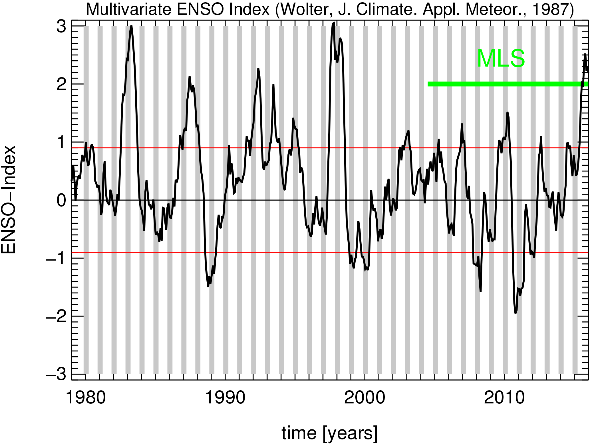
Figure 1Multivariate ENSO Index (MEI) from the NOAA Climate Diagnostic Center, http://www.esrl.noaa.gov/psd/enso/mei (last access: 6 June 2018) (Wolter, 1987). The red lines denote the threshold values (±0.9) defining the El Niño (positive) and La Niña (negative) composites as used in this paper. Grey shading shows winter seasons (December–February, DJF). Figure modified from Konopka et al. (2016).
There are several indices that indicate the phase of ENSO, and they are highly correlated (Pumphrey et al., 2017). Here, the Multivariate ENSO Index (MEI, Fig. 1) from the NOAA (National Oceanic and Atmospheric Administration) Climate Diagnostic Center, http://www.esrl.noaa.gov/psd/enso/mei (last access: 6 June 2018), is used to quantify the ENSO variability (Wolter and Timlin, 2011). MEI is calculated based on sea surface pressure, zonal and meridional components of the surface wind, SST and total cloudiness fraction of the sky over the tropical Pacific. The two phases of ENSO typically show pronounced features in late autumn, winter and early spring (Moron and Gouirand, 2003; McPhaden, 2015). Correspondingly, MEI shows peak values during this period. Negative and positive values of MEI quantify La Niña and El Niño events, respectively.
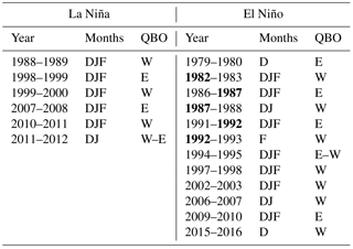
Hereafter, we define two winter composites (December-February, DJF) of ENSO events using the condition MEI < −0.9 for La Niña and MEI > 0.9 for El Niño (red lines in Fig. 1) as discussed in Konopka et al. (2016). The winter months defining these two composites (17 months for 6 La Niña events and 28 months for 12 El Niño) are listed in Table 1. The quasi-biennial oscillation (QBO) phase during the considered months is also listed (http://www.cpc.ncep.noaa.gov/data/indices/qbo.u50.index, last access: 6 June 2018) and shows that our composites are only weakly biased by the westerly phase.
El Niño episodes which last over the whole of the following year, are selected as the special long-lasting El Niño cases and are in bold in Table 1 in black (like during 1987 and 1992). The exceptional El Niño in 1982, which starts in spring 1982 and lasts until autumn 1983, is also considered to be a long-lasting El Niño case (in bold in Table 1). These three cases, as well as the influence of QBO on the results, will be separately discussed in Sect. 5.
Table 1List of all relevant La Niña and El Niño winter months during the period of 1979–2015. In total there are 17 and 28 months for the La Niña and El Niño composites, respectively, which are listed above (DJF for December, January and February). Within the La Niña composite there are 7 months in the easterly phase (E) and 10 months in the westerly phase (W) of the QBO (defined by 30-day smoothed equatorial wind at 50 hPa). For El Niño composites 11 months are in the easterly phase and 17 months are in the westerly phase. The years in bold mark the long-lasting El Niño episodes (for details, see text). Table modified from Konopka et al. (2016).
To study the effect of strong ENSO winters on the UTLS in the following months, we also consider climatologies of “shifted” composites for different seasons (DJF, JFM, FMA, MAM, AMJ, MJJ and JJA); e.g. AMJ represents 4 months after ENSO winters (DJF). The mean value of a composite is defined from the averaged monthly means of its elements. A Monte Carlo significance test is used to investigate whether the La Niña and El Niño composites are statistically different or not. Monte Carlo significance test procedures consist of comparing the observed data with random samples generated in accordance with the hypothesis being tested (Hope, 1968). We call two (La Niña and El Niño) composites statistically different when the significance of the Monte Carlo test for their difference is passed at a 95 % confidence level after at least 1000 iteration steps.
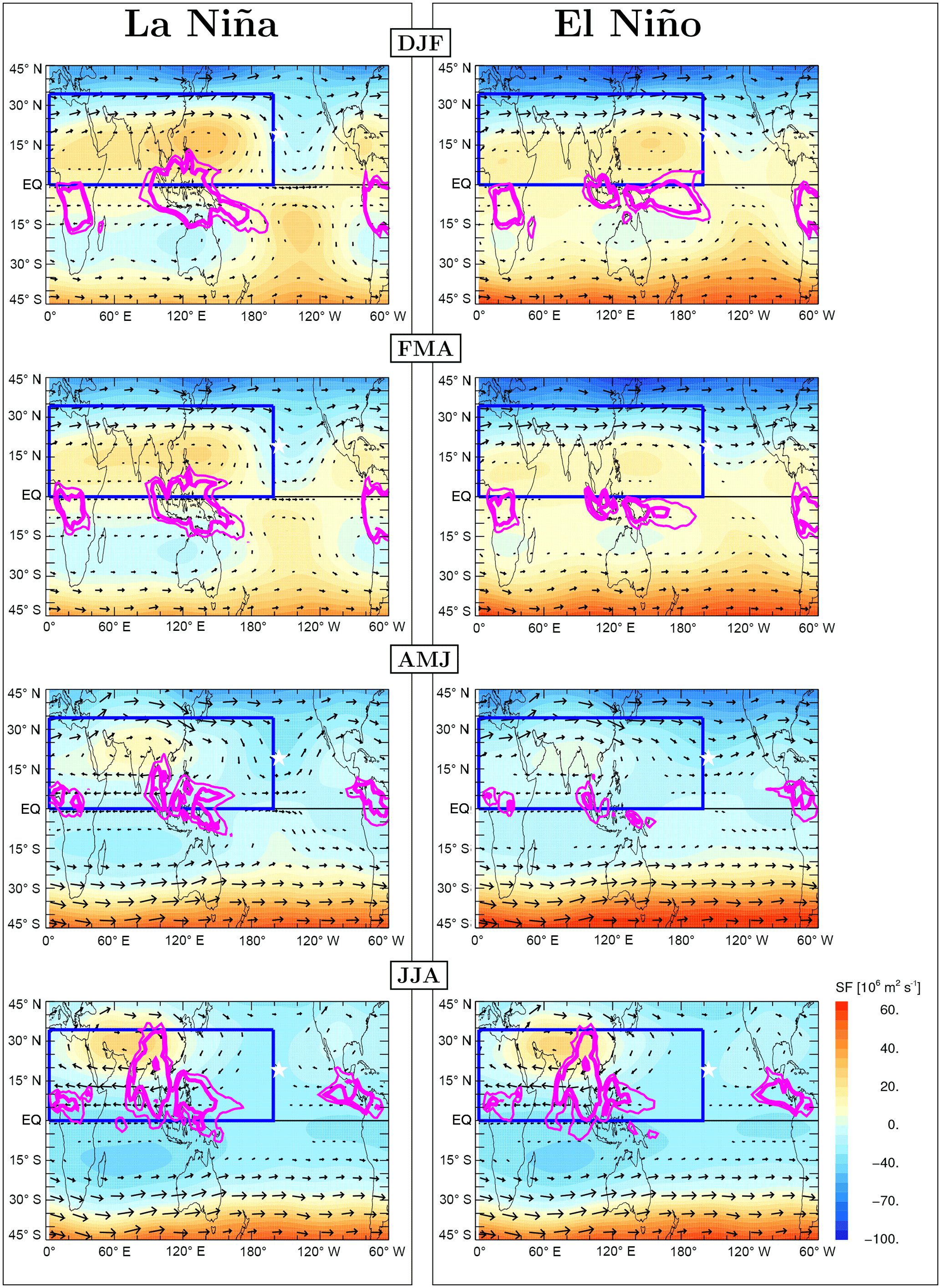
Figure 2Climatologies (composites) of the stream function (SF, in 106 m2 s−1) at θ=380 K calculated from ERA-Interim (1979–2015) for months following La Niña (left) and El Niño (right) winters until summer (from top to bottom). The arrows represent the rotational horizontal wind. Magenta isolines indicate the strong convection regions based on OLR (thick and thin lines represent 210 and 220 W m−2 contours). The blue rectangles mark the locations of strong anticyclone in NH (for details, see text). Hereafter, the star in the figure marks the location of the SHADOZ station (Hilo, Hawaii) where long-term ozonesonde observations are available (see Sect. 4.3).
To quantify ENSO anomalies in the climatological flow patterns, stream function (SF) ψ and velocity potential (VP) χ are calculated (Tanaka et al., 2004) using meteorological data from ERA-Interim reanalysis during 1979–2015 (Dee et al., 2011). According to the Helmholtz theorem, an arbitrary 2-D horizontal flow can be separated into a non-divergent (i.e. rotational) part ua with and a divergent (i.e. irrotational) part ub with , i.e.
where both parts can also be expressed in terms of the potentials ψ and χ. Here, k denotes the unit vector perpendicular to the considered 2-D surface. SF and VP are scalar quantities which are easy to plot and widely applied in meteorology and oceanography to represent large-scale flow fields (see e.g. Evans and Allan, 1992; Kunze et al., 2016). SF quantifies the position and strengths of the cyclones and anticyclones. Following Tanaka et al. (2004), we use VP to represent the Walker circulation and the zonal mean of VP to quantify the Hadley circulation. SF and VP will be divided into El Niño and La Niña composites as described above.
Ozone distributions are used to validate our diagnostic of the flow and to understand the effect of ENSO on the atmospheric composition in the UTLS region. MLS ozone data (version 4.2) and the Hilo (Hawaii) ozonesonde data from Southern Hemisphere ADditional OZonesondes (SHADOZ, Thompson et al., 2007) are used (see http://croc.gsfc.nasa.gov/shadoz, last access: 6 June 2018) as references. MLS measurements provide 8 and 6 months of data for the 3 La Niña and 3 El Niño episodes from 2004 to 2015. Respectively there are 14 and 11 months of data for the 5 La Niña and 5 El Niño events from SHADOZ ozondesondes covering the period 1998–2015. Chemical Lagrangian Model of the Stratosphere (CLaMS) simulations (McKenna et al., 2002; Konopka et al., 2004; Pommrich et al., 2014) driven by the ERA-Interim reanalysis are used to obtain robust statistical composites of ozone (with the same number of La Niña/El Niño months as for SF and VP). Outgoing long-wave radiation (OLR) monthly data from NOAA during 1979–2015 complete our analysis as a proxy for deep convection (see https://www.esrl.noaa.gov/psd/data/gridded/data.interp_OLR.html, last access: 6 June 2018).
In this section, we use the composites of the SF and the VP introduced above to illustrate some ENSO-related differences in the mean flow properties around the tropical tropopause.
3.1 Cyclones and anticyclones
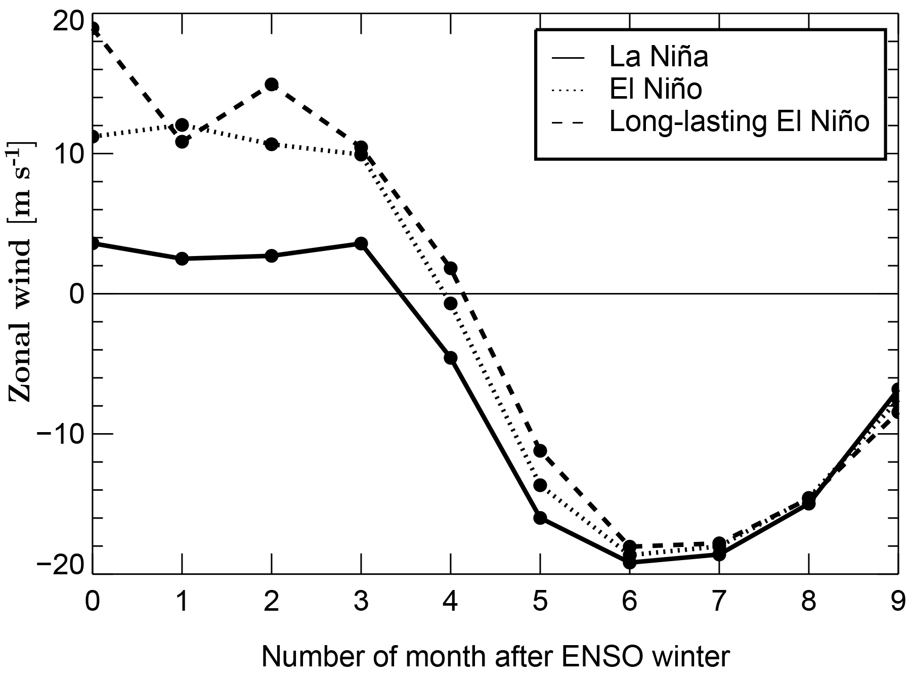
Figure 3Mean zonal wind in the tropics over south-eastern Asia (5∘–20∘ N, 40∘–120∘ E) following La Niña, El Niño and long-lasting El Niño winters at 200 hPa. The transition from positive to negative values marks the onset of the Asian summer monsoon (ASM). The zero mark on the x axis denotes the middle of the DJF season (i.e. 15 January).
Seasonal variations in SF after strong La Niña and El Niño winters are shown in Fig. 2. Here, respective climatologies are plotted at the potential temperature level θ=380 K, which roughly marks the tropopause in the tropics and in the extratropics separates the overworld from the lowermost stratosphere (Holton et al., 1995; Gettelman et al., 2011). The panels in Fig. 2 start from the winter (top, DJF) and end with the summer distribution (bottom, JJA).
Because the divergent part of the flow at θ=380 K is very small compared to its rotational part, isolines of SF approximate the climatological streamlines, whereas the strongest horizontal gradients of SF describe the highest flow velocities. The anticyclones are represented by positive and negative SF values in the NH and Southern Hemisphere (SH), with highest and lowest values corresponding to their centres, respectively. During DJF, the flow in the tropical UTLS between 60∘ E and 120∘ W is dominated by two equatorially symmetric anticyclones resembling the well-known (symmetric) Matsuno–Gill solution with the heat source from convection located symmetrically over the equator (Matsuno, 1966; Gill, 1980; Highwood and Hoskins, 1998).
The climatological sources of heat can be approximated by the lowest values of the OLR. The analogous composites for OLR (magenta contours in Fig. 2) as for the SF are built with respect to La Niña and El Niño conditions. Thus, following the symmetric Matsuno–Gill solution as a proxy, the relevant latent heat sources for the anticyclones originate mainly in the western Pacific, especially during La Niña, and these sources are partially shifted to the east during El Niño events.
Over the course of the following 6 months, as the intertropical convergence zone (ITCZ) moves northwards, these two anticyclones shift to the north-west roughly following the position of convection (Highwood and Hoskins, 1998). The anticyclone in the NH intensifies, starting in May and June, and forms the well-known Asian summer monsoon (ASM) anticyclone during NH summer. In addition a weaker anticyclone in the SH can also be diagnosed. Thus, the summer configuration resembles more a superposition of a symmetric and antisymmetric Matsuno–Gill solution (Gill, 1980; Zhang and Krishnamurti, 2006).
Now we discuss the differences in the large-scale flow in the UTLS caused by ENSO (i.e. differences between the left and the right column of Fig. 2). The most striking difference in DJF is a much weaker meridional disruption of the subtropical jets during El Niño than during La Niña winters, mainly in the NH subtropics between 170∘ E and 70∘ W. At the lower levels (not shown), stratospheric intrusions coincide with regions of the so-called “westerly ducts”, which are much weaker during El Niño (Waugh and Polvani, 2000).
Furthermore, the equatorially symmetric anticyclones are more pronounced for the La Niña composites due to stronger and more localized convection in the western Pacific. These differences are also present during FMA, become smaller during AMJ and disappear during JJA mainly because forcing of the summer dynamics, especially of the ASM, is only weakly related to the winter forcing.
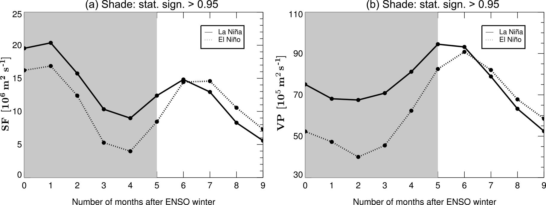
Figure 4The average value of the stream function (a) in the domain of 0∘–35∘ N, 0∘–160∘ W and velocity potential (b) in the domain of 30∘ S–40∘ N, 90∘ E–140∘ W for La Niña (solid line) and El Niño (dotted line) composites at θ=380 K. The grey shading region denotes the period with statistically significant differences between the two composites.
The mean climatological anticyclone in AMJ (Fig. 2) is at the very beginning phase of the ASM anticyclone after El Niño winters, while it develops quickly and strengthens after La Niña winters. We use the transition of the upper-level (at 200 hPa) flow from westerly to easterly winds over south-eastern Asia (5∘–20∘ N, 40∘–120∘ E) to characterize the onset of the monsoon as discussed in Ju and Slingo (1995). By using the shifted composites as in the previous section, it turns out that the onset of the ASM after La Niña is about half a month earlier than after El Niño (Fig. 3). The difference in SF between La Niña and El Niño composites lasts from winter (DJF) to early summer (AMJ) and are insignificant in summer (JJA) as noted earlier.

Figure 5Same as Fig. 2 but for the velocity potential (VP; in 105 m2 s−1) at θ=380 K with arrows denoting the divergent part of the horizontal wind.
To prove the statistical significance of the ENSO anomalies in the SF composites, we compare their mean values averaged over a representative region shown as a blue rectangle in Fig. 2. The domain, defined as 0∘–35∘ N, 0∘–160∘ W, contains the NH anticyclone from winter to summer. The results are shown in the left panel of Fig. 4. The period with statistically different composites is shaded grey. Thus, the NH anticyclone in La Niña years is significantly stronger than in El Niño years within the first 5 months of the year, i.e. until MJJ. This statistical analysis indicates that the influence of ENSO on the anticyclone propagates from winter until early summer. The mean SF difference between La Niña and El Niño composites from winter to early summer is m2 s−1.
3.2 Walker circulation

Figure 6Zonal mean of the velocity potential at θ=360 K defining the Hadley circulation and calculated for La Niña (a) and El Niño composites (b). The difference between La Niña and El Niño composites (c). The average intensity of the Hadley circulation calculated for the domain of 20∘ S–20∘ N (d).
Complementary to SF, the divergent part of the horizontal flow can be described by the VP and is shown in Fig. 5. Note that VP is a factor of 10 smaller than SF, which is consistent with the fact that the non-divergent rather than divergent part dominates the flow at θ=380 K. Following Tanaka et al. (2004), the positive peak of VP indicates the intensity of the Walker circulation and the zonal mean of VP () quantifies the Hadley circulation (see below). The positive values of VP represent the divergence or, using the continuity equation, the strength of the upwelling, while the negative values are related to convergence or downwelling. In this way, the upper branch of the Walker circulation can be diagnosed in Fig. 5. The intensities of the Walker circulation are similar to the results from Tanaka et al. (2004).
The positive peak values of VP lie in the western and central tropical Pacific for La Niña and El Niño DJF climatologies, respectively. They correspond to the locations of rising motion. The mean upwelling (downwelling) activity in La Niña winters is much stronger than in El Niño winters, in agreement with the well-known weakening of the Walker circulation after El Niño events (Wang et al., 2002). In spring (FMA) the differences between the two composites are smaller than in winter. At the beginning of summer (AMJ), the centres of the divergence start to shift from the tropics to the extratropics and the differences become even smaller. In JJA, these centres reach the China Sea. The strengths and positions of the convergence/divergence centres in the La Niña composite are comparable to those of El Niño in that season.
As was done for SF, the statistical significance of the ENSO anomalies in the VP composites is diagnosed in the right panel of Fig. 4. The blue rectangle in Fig. 5, defined as 30∘ S–40∘ N, 90∘ E–140∘ W, represents the region of the ascending branch of the Walker circulation. The mean positive values over this blue rectangle are calculated. The domain allows quantification of the average upwelling of the Walker circulation. The divergence in the La Niña composite is significantly higher than in the El Niño composite within the first 5 months of the year. The mean VP difference between La Niña and El Niño composites from winter to early summer is m2 s−1.
3.3 Hadley circulation
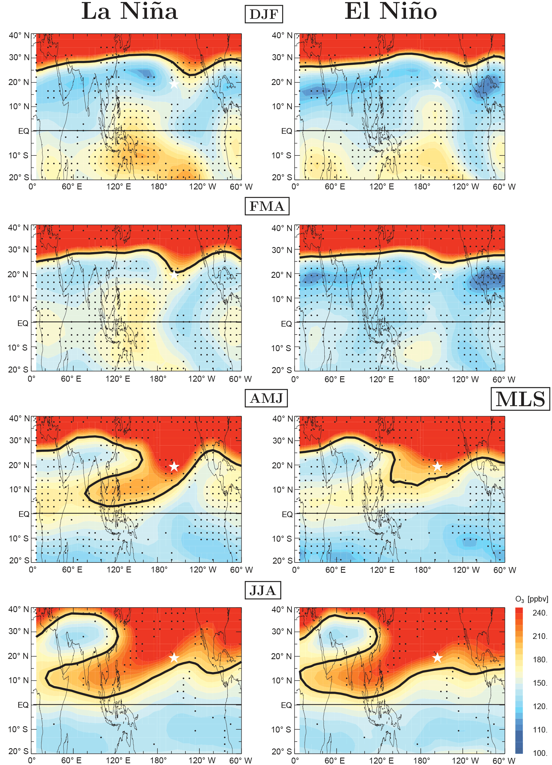
Figure 7Seasonal ozone climatology derived from MLS observations (2004–2015, version 4.2) at θ=380 K for La Niña and El Niño composites from winter to summer months (from top to bottom). Regions with statistically significant differences are marked by the black dots. The black isolines represent ozone of 185 ppbv, which mark the tropopause (see text).
The zonal mean of VP () is used to represent the Hadley circulation (Fig. 6a and b). Note that the peak values of VP are more than three times larger than . In winter, is positive in SH and negative in NH. The positive peaks represent the locations of rising air and correspond to the ITCZ. The negative peaks represent the locations of sinking air. The rising and sinking motions form the mean meridional Hadley circulation. This circulation is weaker after La Niña than after El Niño episodes, and the differences between the La Niña and El Niño composites decrease in summer.
The latitudes of positive peaks show that the rising motion is shifted southwards after El Niño winters compared to La Niña winters. Correspondingly, the ITCZ is located around 4 and 6∘ S for the La Niña and El Niño composites. Figure 6c shows the difference between La Niña and El Niño composites. The upwelling and downwelling after El Niño are much stronger than after La Niña from DJF to MAM. The difference is smaller after AMJ. To check the statistical significance of such differences, the average rising intensity of the Hadley circulation, which is located in the tropics (from 20∘ S to 20∘ N), is calculated (Fig. 6d). The values after El Niño winters are higher than after La Niña winters, especially from DJF to MAM as noted before. The mean difference is about 2×10⁵ m2 s−1, and is insignificant starting from April.
So far we have investigated the influence of ENSO anomalies on the atmospheric circulation, especially on the mean horizontal flow quantified in terms of the SF (Fig. 2) and VP (Fig. 5). Such changes in the atmospheric circulation will also affect the distribution of atmospheric constituents (Randel et al., 2009; Ziemke et al., 2015). Ozone is a sensitive indicator of transport properties in the UTLS region due to its strong vertical and horizontal gradients and its relatively long chemical lifetime. Furthermore, in the sub- and extratropics around the subtropical jet, the ozone distribution is mainly determined by transport rather than by chemistry. In this section, we quantify the impact of ENSO anomalies on the mean ozone distribution based on MLS satellite data, CLaMS simulations and SHADOZ ozonesonde data.
In particular, we now investigate the influence of ENSO on the isentropic in-mixing of high stratospheric ozone values into the TTL (Konopka et al., 2010). In the following, the ozone isoline at the tropopause is used to quantify the effect of isentropic in-mixing at θ=380 K. Thouret et al. (2006) estimated the monthly mean climatological ozone concentration at the tropopause based on MOZAIC measurements. They found a maximum value in May (120 ppbv) and a minimum value in November (65 ppbv). Here, the isoline of 120 ppbv is used as the ozone boundary for CLaMS composites to obtain a conservative estimate of stratospheric influence. MLS ozone has a high bias of ∼ 40 % at 100 hPa in the tropics (Livesey et al., 2017) and even by as much as ∼ 70 % inside the ASM anticyclone (Yan et al., 2016). Therefore, the isoline of 185 ppbv is used as a proxy for the tropopause in the MLS composites.
4.1 MLS composites
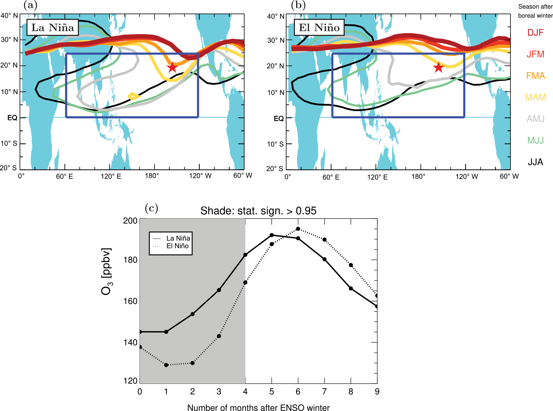
Figure 8(a, b) Isolines of MLS ozone (185 ppbv, black lines in Fig. 7) approximating the tropopause at θ=380 K for different seasons following La Niña (a) and El Niño (b) winters from DJF (red) to JJA (black). (c) The mean concentration of ozone from the blue domain in the top panel (0∘–25∘ N, 60∘ E–120∘ W) marking the region of strongest ENSO-related differences in in-mixing .
Figure 7 shows MLS ozone mixing ratio distributions at θ=380 K from winter to summer after La Niña and El Niño winters. The ozone isoline at the tropopause is represented by the black solid line. During DJF and FMA, the El Niño composite is more zonally symmetric compared to La Niña. This is consistent with the less disturbed subtropical jets after El Niño winters as discussed in the last section. The region of enhanced in-mixing can be recognized as a tongue of high ozone which emerges around 120∘ W, 30∘ N during DJF and is shifted in the following months to the west until the ASM anticyclone forms.
During AMJ, this feature of in-mixing is much more pronounced for the La Niña than for the El Niño composite. This may be related to the differences in the developing process of the ASM anticyclone between La Niña and El Niño shown in Fig. 2. The mean anticyclone in AMJ is in the very first phase after El Niño, while the ASM anticyclone develops more quickly after La Niña and the ozone distribution is affected by a stronger ASM anticyclone during this period. The largest pattern difference between La Niña and El Niño ozone composites occurs during this period, while the SF shows the largest pattern difference in winter (Fig. 2, top). Ozone in-mixing anomalies seem to be delayed compared to the distribution of SF.
The black dots in Fig. 7 provide information about regions with statistically significant differences between La Niña and El Niño composites. We can see that the differences exist almost everywhere, especially in the regions of strong in-mixing described above. During the mature phase of the ASM anticyclone (JJA), the number of black dots decrease strongly, but there is still a region of significant in-mixing differences on the ozone tongue as well as on the extratropical side of the tropopause. We will return to this point later. Ozone values in the centre of the ASM anticyclone are lower after La Niña than after El Niño in JJA, which is consistent with the similar differences in the SF (cf. Fig. 2).

Figure 9Zonally averaged (10∘–130∘ E) time series of MLS ozone at θ=380 K (version 4.2; for more details see Santee et al., 2017) over the course of these 3 representative years (a–c) 2008 (after La Niña winter), 2009 (a normal year) and 2010 (after El Niño winter).
The isolines of ozone representing the tropopause are combined together in Fig. 8a and b to illustrate the pattern of the seasonality of the ENSO-related differences in in-mixing. To quantify such differences, the mean concentration inside the blue domain 0∘–25∘ N, 60∘ E–120∘ W is calculated and shown in Fig. 8c. The grey shading highlights the seasons with statistically significant differences between La Niña and El Niño composites, which are from DJF to AMJ. The average results inside the in-mixed region attest that ozone concentration after El Niño is about 16 ppbv lower than after La Niña from winter (DJF) to early summer (AMJ). The difference is a manifestation of the influence of stronger Hadley and BD circulations and weaker in-mixing after El Niño than after La Niña on the horizontal distribution of ozone around the tropopause (Randel et al., 2009; Calvo et al., 2010; Konopka et al., 2016). Starting from summer, the difference in ozone distribution between El Niño and La Niña is statistically insignificant. Starting in JJA, the concentration of in-mixed ozone after El Niño years is even higher than after La Niña years.
To better understand such statistical differences, now we investigate the MLS observations in more detail for three example years which are representative of typical El Niño, La Niña and neutral conditions. Following the method described in Santee et al. (2017), in Fig. 9 we plot the time series of the zonally averaged ozone (10∘–130∘ E) at 380 K during 2008 (i.e. after La Niña), 2009 (i.e. during a neutral year) and 2010 (i.e. after El Niño). Over the course of these 3 representative years, the differences in ozone between the equator and ∼ 30∘ N mainly result from different intensities of in-mixing and the BD circulation. Specifically, the ozone mixing ratios after El Niño winter (2010) are much lower than after La Niña winter (2008) or even during a normal year (2009), with a negative anomaly persisting from January to June, supporting our statistical results in Figs. 7 and 8. The isentropic intrusions transport less ozone from high latitudes to the tropics following El Niño winters.
However, there is more in-mixed ozone in 2010 than in 2008 and 2009 from June to September. This could be a consequence of the differences in the BD circulation (stronger after El Niño than after La Niña winters), which may cause higher ozone values in the northern extratropics and, consequently, stronger isentropic gradients of ozone after El Niño winters. It means that under El Niño conditions, transport of ozone-rich air from the extratropics to the tropics is inhibited during winter and spring by the strong subtropical jet, but transport to the tropics may occur later in summer when the subtropical jet is weaker. We will come back to this point in Sect. 5.
4.2 In-mixing from CLaMS
As discussed in Konopka et al. (2016, Fig. 5), CLaMS reproduces the ENSO anomalies in ozone observed by MLS fairly well. However, at the time of writing the MLS composites cover only 11 years with very few strong El Niño and La Niña events. Using CLaMS ozone, we are able to extend our period to 37 years from 1979 to 2015 and obtain statistically more robust results.

Figure 11Composites of the ozonesonde measurements from SHADOZ in Hilo, Hawaii 19.43∘ N, 155.04∘ W during 1998–2015. Black and red lines represent the seasonal mean profiles for La Niña and El Niño composites. The shading indicates the standard deviation of the mean. The dotted and dashed lines represent the results for subcomposites defined by the westerly and easterly phases of the QBO.
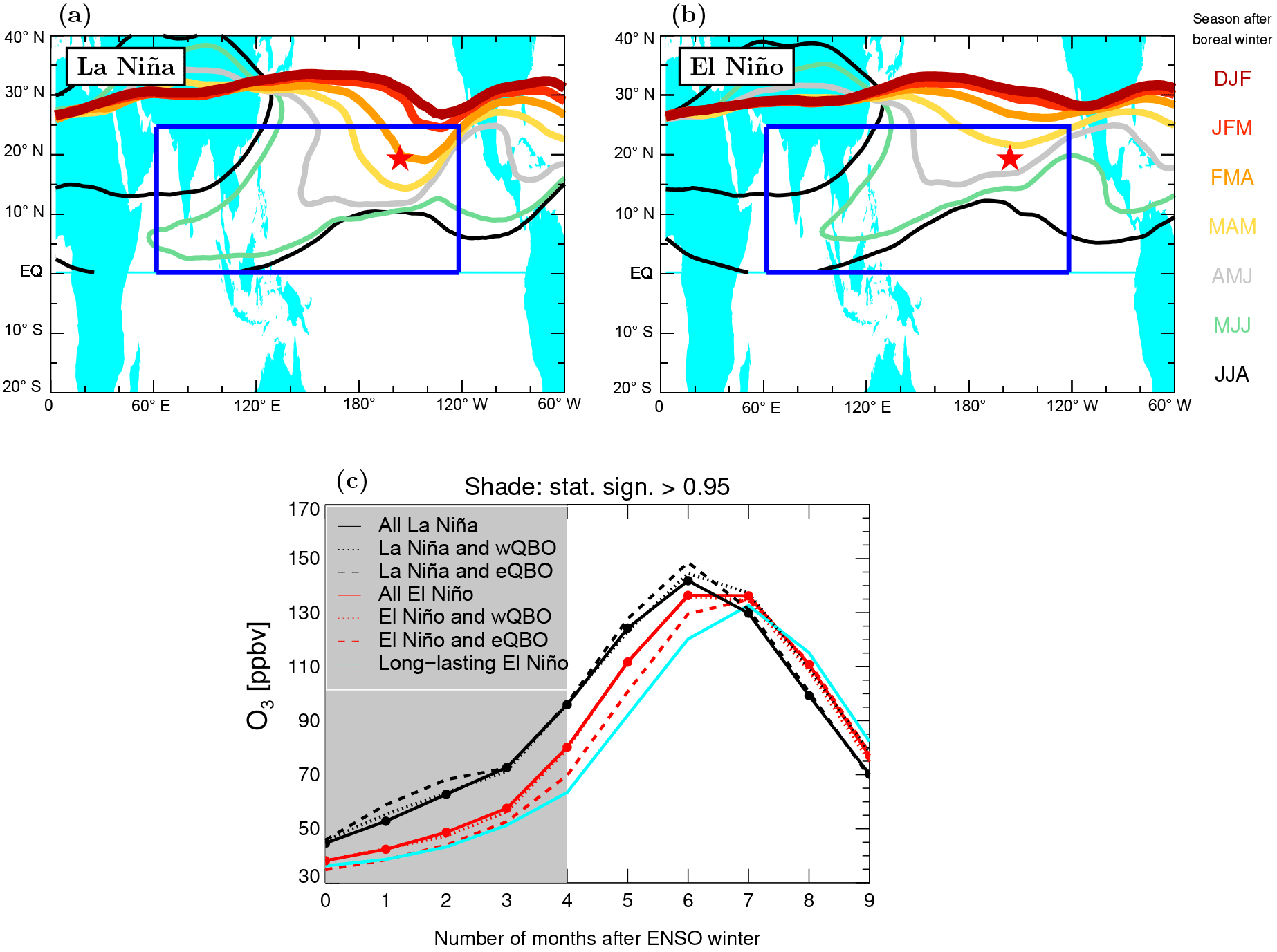
Figure 10 (top) shows the same type of distribution as Fig. 8 (top) but for 37 years of CLaMS ozone simulations and with the tropopause defined by the ozone isoline with 120 ppbv. The ozone concentrations from CLaMS simulations are about 50 ppbv lower than MLS measurements at θ=380 K, in part because of the zero ozone boundary condition at the ground, but they show similar patterns to MLS ozone. The CLaMS ozone distributions also show in-mixing activity over the eastern and central Pacific in subsequent months following La Niña winters, with more zonally symmetric features during months following El Niño. The signatures of in-mixing over the tropical Pacific are much stronger after the onset of the ASM anticyclone (AMJ) for both composites and extend deeper into the tropics after La Niña than after El Niño winters. The differences disappear in JJA.
The largest difference between the ENSO composites exists around the eastern flank of the ASM anticyclone. To quantify this difference from CLaMS simulations, the mean concentrations in the blue domain are calculated (i.e. in the same way as for MLS) and are shown as solid black and red lines in Fig. 10c for La Niña and El Niño composites (the results for the long-lasting El Niño years and for the subcomposites related to the different QBO phases are also shown and will be discussed in Sect. 5). As for the MLS composites, the CLaMS results show a similar pattern with less in-mixed ozone from El Niño winters to early summer and more in-mixed ozone in the late summer and autumn, although statistically significant differences can only be found until AMJ (grey shading). The ozone concentration after El Niño is about 12 ppbv lower than after La Niña. This difference obtained from CLaMS simulations for the time period 1979–2015 is slightly smaller than from MLS measurements for the time period 2004–2015.
4.3 In-mixing from SHADOZ
MLS measurements and CLaMS simulations as described above provide the ENSO-related differences in the horizontal distribution of ozone. The vertical influence of ENSO anomalies on the ozone distribution near the tropopause can also be inferred from the ozonesonde data obtained at the SHADOZ station in Hilo, Hawaii 19.43∘ N, 155.04∘ W (marked with a star in Figs. 2, 7, 8 and 10) from 1998 to 2015. Hilo is located in the central Pacific at the edge of the climatological position of the anticyclone in winter (see Fig. 2). The air over Hilo is strongly affected by the meridional disruption of the subtropical jet from winter (DJF) to early summer (AMJ) following La Niña winters, while it is within the tropics following El Niño winters.
The resolution of the SHADOZ ozone profiles is not the same for the whole period, so the data are degraded to the vertical resolution of 200 m for all years to calculate the ENSO composites introduced in Sect. 2.
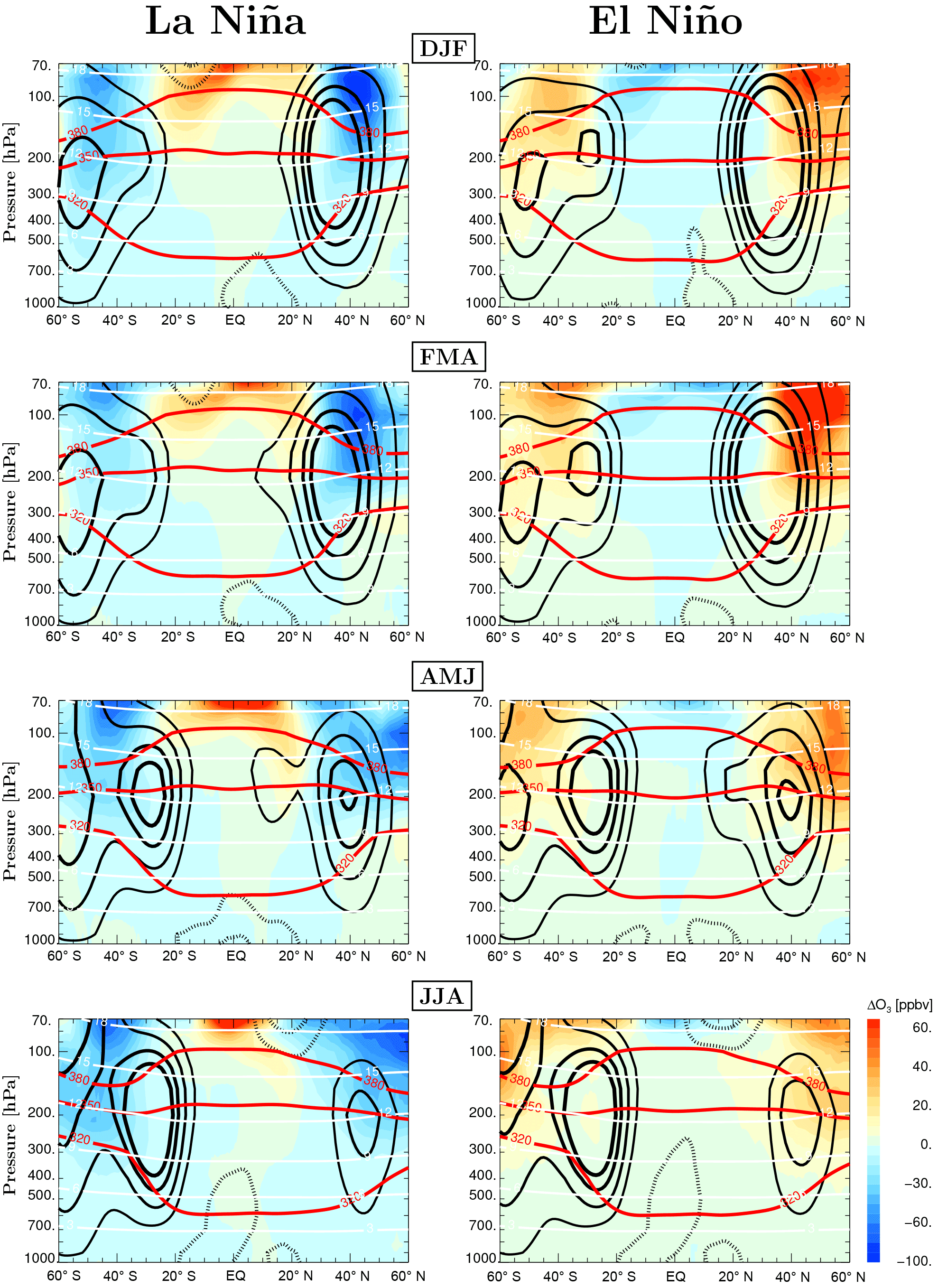
Figure 12The anomalies of zonally averaged ozone in the western and central Pacific (120∘ E, 120∘ W) from DJF to JJA based on CLaMS simulations covering 1979–2015. The solid and dashed lines are the zonal means of the westerlies (10, 17, 24 and 30 m s−1) and easterlies (−5, −10 and −20 m s−1). Red and white lines represent potential temperature (K) and geopotential height (km).
Figure 11 shows the ENSO-related seasonal variation in ozone with altitude over Hilo (red and black solid profiles), as well as their variability due to the QBO phase (dotted and dashed lines), which will be discussed in the next section.
The mean ozone profiles during and after El Niño show a characteristic S-shaped structure for all the seasons, with the lowest value near the surface, a maximum near 6 km, a minimum near 12–13 km, and a subsequent increase toward stratospheric values. The minimum ozone concentrations at ∼ 12–13 km are located at the level of main convective outflow and are therefore caused by uplift of tropospheric air (Folkins et al., 2002; Thompson et al., 2012). On the other hand, the ozone profiles from La Niña winters do not show such a minimum. On average, the ozone concentration for La Niña is about 44 ppbv higher than for El Niño from 9 to 18 km in DJF (top left). The ozone concentration differences between La Niña and El Niño during FMA and AMJ (top right and bottom left) are smaller, with mean values around 38 and 20 ppbv. Finally, there is no clear difference between these two composites during JJA (bottom right).
The results from SHADOZ indicate that the air masses are more affected by in-mixing following La Niña years, and that this effect is not only confined to the region around 380 K (≈ 15 km) but can be diagnosed throughout the whole UTLS region. Especially in winter, ENSO-related anomalies in the ozone profile are quite large (from 9 to 21 km) compared to other seasons. The influence lasts from winter (DJF) to early summer (AMJ) but vanishes during JJA. Interestingly, the ENSO anomaly of in-mixing changes polarity in the middle troposphere below 9 km. We discuss this point in the following section.
The ENSO anomaly induces two types of variability in the global ozone distribution: on the one hand, the stronger Hadley/BD circulation during and after El Niño winters transports less ozone into the TTL and more ozone in the extratropical lower stratosphere and, consequently, stronger latitudinal gradients of ozone on all isentropes in the UTLS region have to be expected (Randel et al., 2009; Calvo et al., 2010; Konopka et al., 2016). On the other hand, a less disturbed subtropical jet after El Niño more effectively suppresses the isentropic in-mixing of ozone into the tropics during winter and spring (this effect was extensively shown in this paper), while during late summer and autumn higher ozone values, although less frequently, can be in-mixed into the TTL.
The latter effect can be seen in the MLS observations at θ=380 K (Fig. 9) and are mainly caused by isentropic in-mixing around the eastern flank of the ASM anticyclone. This effect can also be inferred from our statistical analysis of the enhanced mean ozone values in the blue region discussed in Fig. 8. The values shown in Figs. 8 and 10 for MLS and CLaMS suggest that during late summer and autumn the in-mixed ozone is higher after El Niño than after La Niña winters, although we cannot prove the statistical robustness of this result. In addition, all the SHADOZ mean profiles around 3–9 km (Fig. 11) show higher ozone for El Niño than for La Niña composites.
To discuss this point in more detail, Fig. 12 shows from top to bottom the seasonal results of the zonal mean (120∘ E–120∘ W) ozone anomalies after La Niña and El Niño from the surface to 70 hPa as derived from the respective CLaMS composites. The depicted ozone anomalies are mainly due to changes in the Hadley/BD circulation, with the largest negative (positive) changes in the TTL and positive (negative) changes in the lower extratropical stratosphere mainly in the NH following El Niño (La Niña) winters. Although the largest ozone anomalies can be found in DJF and FMA, their absolute values weaken in the following months, especially in the tropics. In addition, the positive anomaly in the north of the subtropical jets (black lines in Fig. 12) under El Niño conditions propagates downwards into the middle troposphere, mainly in the NH.
We conclude that enhanced tropical upwelling in DJF and FMA following El Niño transports ozone-poor air from the surface to the TTL. Likewise, the enhanced downwelling poleward of the subtropical jets following El Niño transports ozone-rich air from the stratosphere to the sub- and extratropical middle troposphere. The higher ozone as observed by MLS at θ=380 K during late summer 2010 (Fig. 9) as well as the higher ozone in the middle troposphere below 9 km in Hilo during DJF and FMA following El Niño (Fig. 11) may be partially related to the isentropic transport of ozone-rich air from the stratosphere. While in the first case, the isentropic transport happens above the jet, mainly on the eastern flank of the ASM anticyclone, in the second case the isentropic pathway of transport is related to the isentropes below the jet, i.e. to the θ surfaces between 320 and 340 K (Newell et al., 1999; Thouret et al., 2001; Hayashi et al., 2008; Pan et al., 2015).
Inspired by the work of Chowdary et al. (2016) showing decreasing Indian summer monsoon rainfall after long-lasting El Niño events, episodes which last until the autumn or over the whole year following the El Niño winters are now selected (i.e. the years 1982, 1987 and 1992 listed in Table 1). Here, we investigate whether their mean influence on the atmospheric circulation and on the ozone distribution, although not statistically significant, will increase the El Niño-related effects derived in the previous sections. Table 2 shows the peak values of SF, VP and the Hadley circulation found inside the blue domains in Figs. 2, 5 and 6.
Table 2List of the maximum strength of the NH anticyclone (SF in 106 m2 s−1), Walker circulation (VP in 105 m2 s−1) and Hadley circulation (HC in 105 m2 s−1) after La Niña, El Niño and long-lasting El Niño found inside the blue domains in Figs. 2, 5 and 6.
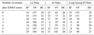
Indeed, SF, VP and the Hadley circulation averaged over these 3 years show the strongest anomalies if compared to all El Niño years. In particular, the ASM anticyclone is weaker and the Hadley circulation is stronger for most considered months following the long-lasting El Niño winters. The onset date of the ASM after long-lasting El Niños is even slightly later than after the other El Niño winters (Fig. 3). Accordingly, the ozone concentrations in the tropics are less disturbed by isentropic intrusions from the subtropics. Consequently, the lowest ozone concentrations are detected in the blue domain in Fig. 10 until the end of summer, at which time ozone following long-lasting El Niños switches to having the highest values in early autumn (cyan line in Fig. 10). This indicates that if El Niño does not decay until the following summer, its influence on the ASM anticyclone and ozone will last longer.
Neu et al. (2014) found that the superposition of El Niño and easterly QBO phase increases ozone flux from the stratosphere into the troposphere, resulting in enhanced tropospheric ozone values in midlatitudes. The opposite effect occurs for the combination of La Niña and westerly QBO phase. Motivated by this study, we investigate how the QBO phase affects our results. Table 1 shows that La Niña winters are almost equally affected by westerly and easterly QBO phases, while during El Niño the westerly QBO phase occurs more often. To quantify the potential influence of the QBO phase, we compare the difference between La Niña and El Niño subcomposites defined by the westerly and easterly phases. The CLaMS results in the blue rectangle at 380 K (Fig. 10c) show that the ozone concentration after La Niña events is higher than after El Niño events during both phases of the QBO, but their difference is larger during the easterly than during the westerly QBO phase. Similarly, the SHADOZ ozone data (Fig. 11) show that the ozone concentration after La Niña events is higher (lower) than after El Niño events in the UTLS (middle troposphere) during both phases of the QBO, while the respective subcomposites show larger differences during the easterly than during the westerly phase. This indicates that our results on the ENSO effects are robust, but the difference will be enhanced (weakened) during the easterly (westerly) phase of the QBO.
ENSO typically shows the strongest signal in boreal winter, but it can affect the atmospheric circulation and constituent distributions until the next autumn. To quantify the influence of ENSO on the atmosphere from a dynamical perspective, the stream function (SF) and the velocity potential (VP) are introduced. SF and VP represent the divergence-free and the rotation-free parts of the horizontal wind field, respectively. The results show that the subtropical jets after El Niño winters are more zonally symmetric than after La Niña winters. Furthermore, the meridional disruption of the subtropical jets during El Niño are weaker compared to La Niña winters. The anticyclonic circulation in the tropics following El Niño is weaker than following La Niña. The strength of the ASM anticyclone after El Niño is slightly weaker than after La Niña in early boreal summer, and the onset date in El Niño years is about half a month later than in La Niña years. VP after El Niño is weaker than after La Niña from winter to early summer because of the weaker Walker circulation in El Niño years. The Hadley circulation after El Niño is much stronger than after La Niña from winter to spring.
The anomalies in the atmospheric circulation caused by ENSO also affect the distribution of atmospheric composition. MLS satellite measurements (2004–2015) and CLaMS simulations (1979–2015) are used to analyse the influence of ENSO on the ozone distribution in the vicinity of the tropopause (380 K). The results from CLaMS simulations show similar patterns to the MLS measurements. In both, ozone patterns after La Niña winters and springs show in-mixing over the eastern and central Pacific, while the ozone patterns after El Niño winters and springs are more zonally symmetric. The in-mixing difference between La Niña and El Niño is striking during the onset of the ASM anticyclone (AMJ). Intrusions from the high-latitude stratosphere reach much deeper into the tropics after La Niña winters than after El Niño winters. This indicates that the ozone anomaly lags behind the atmospheric circulation anomaly in El Niño and La Niña winters by about 4 months. Based on the ozonesonde data from SHADOZ (1998–2015) in Hilo, Hawaii, the vertical impact of ENSO on the ozone distribution is investigated. The well-known vertical S-shaped structure only exists in the ozone profiles following El Niño but not La Niña from winter to early summer. The ozone concentration in the UTLS after El Niño is lower than after La Niña from DJF to AMJ. Our results demonstrate that the air masses over Hilo following La Niña encounter stronger (weaker) in-mixing in the UTLS (middle troposphere) compared to El Niño.
Weaker in-mixing and stronger Hadley circulation due to El Niño cause lower ozone mixing ratios in the tropical UTLS compared to La Niña from winter to early summer. However, the in-mixed ozone following El Niño winters may become higher in the subtropical middle troposphere as well as in the TTL in late summer and autumn. This effect is related to a stronger Hadley/BD circulation after El Niño compared to La Niña, which may cause higher ozone values in the extratropics and, consequently, stronger isentropic and meridional gradients of ozone after El Niño winters. The duration and intensity of the El Niño-related anomalies are amplified only if the long-lasting episodes are considered. The ENSO-related anomalies are enhanced (weakened) during the easterly (westerly) phase of the QBO.
The stream function, velocity potential and CLaMS model data may be requested from the authors (x.yan@fz-juelich.de or p.konopka@fz-juelich.de). The ENSO MEI index data can be obtained from the website http://www.esrl.noaa.gov/psd/enso/mei/ (last access: 6 June 2018). The QBO data were freely downloaded from http://www.cpc.ncep.noaa.gov/data/indices/qbo.u50.index (last access: 6 June 2018). The OLR data are available at the website https://www.esrl.noaa.gov/psd/data/gridded/data.interp_OLR.html (last access: 6 June 2018). The MLS version 4.2 data can be obtained from the MLS website https://mls.jpl.nasa.gov. The SHADOZ ozonesonde data are available at the website http://croc.gsfc.nasa.gov/shadoz (last access: 6 June 2018).
The authors declare that they have no conflict of interest.
This work was supported by the Strategic Priority Research Program of the
Chinese Academy of Sciences, grant no. XDA2006010203, the National Natural
Science Foundation of China, grant no. 91337214, 41675040 and the
International Postdoctoral Exchange Fellowship Program 2015 under grant no.
20151011. The European Centre for Medium-Range Weather Forecasts (ECMWF)
provided meteorological analysis for this study. OLR and ENSO MEI index data
are provided by NOAA. Ozonesonde data are provided through the SHADOZ
database. Work at the Jet Propulsion Laboratory, California Institute of
Technology, was carried out under a contract with the National Aeronautics
and Space Administration. We would like to thank Suvarna Fadnavis for some
discussions which motivated us to do this work. The stream function and
velocity potential are calculated based on the method from Hiroshi L. Tanaka.
Excellent programming support was provided by Nicole Thomas.
The article processing charges for this open-access
publication were covered by a Research
Centre
of the Helmholtz Association.
Edited by:
Martin Dameris
Reviewed by: three anonymous referees
Bannister, R. N., O'Neill, A., Gregory, A. R., and Nissen, K. M.: The role of the south-east Asian monsoon and other seasonal features in creating the “tape-recorder” signal in the Unified Model, Q. J. R. Meteorol. Soc., 130, 1531–1554, 2004. a
Bjerknes, J.: Atmospheric teleconnections from the equatorial Pacific, Mon. Weather. Rev., 97, 163–172, 1969. a, b
Calvo, N., Garcia, R. R., Randel, W. J., and Marsh, D.: Dynamical mechanism for the increase in tropical upwelling in the lowermost tropical stratosphere during warm ENSO events, J. Atmos. Sci., 67, 2331–2340, https://doi.org/10.1175/2010JAS3433.1, 2010. a, b, c
Chen, P.: Isentropic cross-tropopause mass exchange in the extratropics, J. Geophys. Res., 100, 16661–16673, 1995. a
Chowdary, J. S., Harsha, H. S., Gnanaseelan, C., Srinivas, G., Parekh, A., Pillai, P., and Naidu, C. V.: Indian summer monsoon rainfall variability in response to differences in the decay phase of El Niño, Clim. Dynam., 48, 2707–2727, https://doi.org/10.1007/s00382-016-3233-1, 2016. a
Dee, D. P., Uppala, S. M., Simmons, A. J., Berrisford, P., Poli, P., Kobayashi, S., Andrae, U., Balmaseda, M. A., Balsamo, G., Bauer, P., Bechtold, P., Beljaars, A. C. M., van de Berg, L., Bidlot, J., Bormann, N., Delsol, C., Dragani, R., Fuentes, M., Geer, A. J., Haimberger, L., Healy, S. B., Hersbach, H., Holm, E. V., Isaksen, L., Kallberg, P., Koehler, M., Matricardi, M., McNally, A. P., Monge-Sanz, B. M., Morcrette, J.-J., Park, B.-K., Peubey, C., de Rosnay, P., Tavolato, C., Thepaut, J.-N., and Vitart, F.: The ERA-Interim reanalysis: configuration and performance of the data assimilation system, Q. J. R. Meteorol. Soc., 137, 553–597, https://doi.org/10.1002/qj.828, 2011. a
Dethof, A., O'Neill, A., Slingo, J. M., and Smit, H. G. J.: A mechanism for moistening the lower stratosphere involving the Asian summer monsoon, Q. J. R. Meteorol. Soc., 556, 1079–1106, 1999. a
Dunkerton, T. J.: Evidence of meridional motion in the summer lower stratosphere adjacent to monsoon regions, J. Geophys. Res., 100, 16675–16688, 1995. a
Evans, J. L. and Allan, R. J.: El Nino/southern oscillation modification to the structure of the monsoon and tropical cyclone activity in the Australasian region, Int. J. Climatol., 12, 611–623, 1992. a
Folkins, I., Braun, C., Thompson, A. M., and Witte, J.: Tropical ozone as an indicator of deep convection, J. Geophys. Res.-Atmos., 107, 13–1–ACH 13–10, https://doi.org/10.1029/2001JD001178, 2002. a
Fu, R., Hu, Y., Wright, J. S., Jiang, J. H., Dickinson, R. E., Chen, M., Filipiak, M., Read, W. G., Waters, J. W., and Wu, D. L.: Short circuit of water vapor and polluted air to the global stratosphere by convective transport over Tibetian Plateau, P. Natl. Acad. Sci. USA, 103, 5664–5669, 2006. a
Fueglistaler, S., Bonazzola, M., Haynes, P. H., and Peter, T.: Stratospheric water vapor predicted from the Lagrangian temperature history of air entering the stratosphere in the tropics, J. Geophys. Res., 110, D08107, https://doi.org/10.1029/2004JD005516, 2005. a
Garfinkel, C. I., Hurwitz, M. M., Oman, L. D., and Waugh, D. W.: Contrasting Effects of Central Pacific and Eastern Pacific El Nino on stratospheric water vapor, Geophys. Res. Lett., 40, 4115–4120, https://doi.org/10.1002/grl.50677, 2013. a
Gettelman, A., Hoor, P., Pan, L. L., Randel, W. J., Hegglin, M. I., and Birner, T.: The extratropical upper troposphere and lower stratosphere, Rev. Geophys., 49, RG3003, https://doi.org/10.1029/2011RG000355, 2011. a
Gill, A. E.: Some simple solutions for heat-induced tropical circulation, Q. J. R. Meteorol. Soc., 106, 447–462, 1980. a, b
Hayashi, H., Kita, K., and Taguchi, S.: Ozone-enhanced layers in the troposphere over the equatorial Pacific Ocean and the influence of transport of midlatitude UT/LS air, Atmos. Chem. Phys., 8, 2609–2621, https://doi.org/10.5194/acp-8-2609-2008, 2008. a
Haynes, P. and Shuckburgh, E.: Effective diffusivity as a diagnostic of atmospheric transport, 2, Troposphere and lower stratosphere, J. Geophys. Res., 105, 22795–22810, 2000. a
Highwood, E. J. and Hoskins, B. J.: The tropical tropopause, Q. J. R. Meteorol. Soc., 124, 1579–1604, 1998. a, b
Holton, J. R., Haynes, P., McIntyre, M. E., Douglass, A. R., Rood, R. B., and Pfister, L.: Stratosphere-troposphere exchange, Rev. Geophys., 33, 403–439, 1995. a
Hope, A. C. A.: A Simplified Monte Carlo Significance Test Procedure, J. Roy. Stat. Soc. B. Met., 30, 582–598, 1968. a
Ju, J. and Slingo, J.: The Asian summer monsoon and ENSO, Q. J. R. Meteorol. Soc., 121, 1133–1168, 1995. a, b
Kawamura, R.: A Possible Mechanism of the Asian Summer Monsoon-ENSO Coupling, J. Meteorol. Soc. Jpn., 76, 1009–1027, 1998. a
Konopka, P., Steinhorst, H.-M., Grooß, J.-U., Günther, G., Müller, R., Elkins, J. W., Jost, H.-J., Richard, E., Schmidt, U., Toon, G., and McKenna, D. S.: Mixing and Ozone Loss in the 1999–2000 Arctic Vortex: Simulations with the 3-dimensional Chemical Lagrangian Model of the Stratosphere (CLaMS), J. Geophys. Res., 109, D02315, https://doi.org/10.1029/2003JD003792, 2004. a
Konopka, P., Grooß, J.-U., Günther, G., Ploeger, F., Pommrich, R., Müller, R., and Livesey, N.: Annual cycle of ozone at and above the tropical tropopause: observations versus simulations with the Chemical Lagrangian Model of the Stratosphere (CLaMS), Atmos. Chem. Phys., 10, 121–132, https://doi.org/10.5194/acp-10-121-2010, 2010. a, b
Konopka, P., Ploeger, F., Tao, M., and Riese, M.: Zonally resolved impact of ENSO on the stratospheric circulation and water vapor entry values, J. Geophys. Res.-Atmos., 121, 11486–11501, 2016. a, b, c, d, e, f, g, h
Krüger, K., Tegtmeier, S., and Rex, M.: Long-term climatology of air mass transport through the Tropical Tropopause Layer (TTL) during NH winter, Atmos. Chem. Phys., 8, 813–823, https://doi.org/10.5194/acp-8-813-2008, 2008. a
Kunze, M., Braesicke, P., Langematz, U., and Stiller, G.: Interannual variability of the boreal summer tropical UTLS in observations and CCMVal-2 simulations, Atmos. Chem. Phys., 16, 8695–8714, https://doi.org/10.5194/acp-16-8695-2016, 2016. a
Liess, S. and Geller, M. A.: On the relationship between QBO and distribution of tropical deep convection, J. Geophys. Res., 117, D03108, https://doi.org/10.1029/2011JD016317, 2012. a
Livesey, N. J., Read, W. G., Wagner, P. A., Froidevaux, L., Lambert, A., Manney, G. L., Valle, L. F. M., Pumphrey, H. C., Santee, M. L., Schwartz, M. J., Wang, S., Fuller, R. A., Jarnot, R. F., Knosp, B. W., and Martinez, E.: Version 4.2x Level 2 data quality and description document, available at: https://mls.jpl.nasa.gov/data/v4-2_data_quality_document.pdf (last access: 6 June 2018), 2017. a
Matsuno, T.: Quasi-geostrophic motopns in the equatorial area, J. Meteorol. Soc. Jpn., 44, 25–42, 1966. a
McKenna, D. S., Konopka, P., Grooß, J.-U., Günther, G., Müller, R., Spang, R., Offermann, D., and Orsolini, Y.: A new Chemical Lagrangian Model of the Stratosphere (CLaMS): 1. Formulation of advection and mixing, J. Geophys. Res., 107, 4309, https://doi.org/10.1029/2000JD000114, 2002. a
McPhaden, M. J.: Playing hide and seek with El Nino, Nat. Clim. Change, 5, 791–795, 2015. a, b
McPhaden, M. J., Zebiak, S. E., and Glantz, M. H.: ENSO as an integrating concept in Earth science, Science, 314, 1740–1745, 2006. a
Moron, V. and Gouirand, I.: Seasonal modulation of the El Niño-southern oscillation relationship with sea level pressure anomalies over the North Atlantic in October–March 1873–1996, Int. J. Climatol., 23, 143–155, https://doi.org/10.1002/joc.868, 2003. a, b
Müller, S., Hoor, P., Bozem, H., Gute, E., Vogel, B., Zahn, A., Bönisch, H., Keber, T., Krämer, M., Rolf, C., Riese, M., Schlager, H., and Engel, A.: Impact of the Asian monsoon on the extratropical lower stratosphere: trace gas observations during TACTS over Europe 2012, Atmos. Chem. Phys., 16, 10573–10589, https://doi.org/10.5194/acp-16-10573-2016, 2016. a
Neu, J. L., Flury, T., Manney, G. L., Santee, M. L., Livesey, N. J., and Worden, J.: Tropospheric ozone variations governed by changes in stratospheric circulation, Nat. Geosci., 7, 340–344, https://doi.org/10.1038/ngeo2138, 2014. a
Newell, R. E., Thouret, V., Cho, J. Y. N., Stoller, P., Marenco, A., and Smit, H. G.: Ubiquity of quasi-horizontal layers in the troposphere, Nature, 398, 316–319, 1999. a
Pan, L. L., Honomichl, S. B., Randel, W. J., Apel, E. C., Atlas, E. L., Beaton, S. P., Bresch, J. F., Hornbrook, R., Kinnison, D. E., Lamarque, J. F., Saiz-Lopez, A., Salawitch, R. J., and Weinheimer, A. J.: Bimodal distribution of free tropospheric ozone over the tropical western Pacific revealed by airborne observations, Geophys. Res. Lett., 42, 7844–7851, 2015. a
Park, M., Randel, W. J., Gettelman, A., Massie, S. T., and Jiang, J. H.: Transport above the Asian summer monsoon anticyclone inferred from Aura Microwave Limb Sounder tracers, J. Geophys. Res.-Atmos., 112, D16309, https://doi.org/10.1029/2006JD008294, 2007. a
Park, M., Randel, W. J., Emmons, L. K., Bernath, P. F., Walker, K. A., and Boone, C. D.: Chemical isolation in the Asian monsoon anticyclone observed in Atmospheric Chemistry Experiment (ACE-FTS) data, Atmos. Chem. Phys., 8, 757–764, https://doi.org/10.5194/acp-8-757-2008, 2008. a
Philander, S., Holton, J., and Dmowska, R.: El Nino, La Nina, and the Southern Oscillation, 46, International Geophysics, Academic Press, Cambridge, 1989. a
Ploeger, F., Konopka, P., Müller, R., Fueglistaler, S., Schmidt, T., Manners, J. C., Grooß, J.-U., Günther, G., Forster, P. M., and Riese, M.: Horizontal transport affecting trace gas seasonality in the Tropical Tropopause Layer (TTL), J. Geophys. Res., 117, D09303, https://doi.org/10.1029/2011JD017267, 2012. a
Ploeger, F., Günther, G., Konopka, P., Fueglistaler, S., Müller, R., Hoppe, C., Kunz, A., Spang, R., Grooß, J.-U., and Riese, M.: Horizontal water vapor transport in the lower stratosphere from subtropics to high latitudes during boreal summer, J. Geophys. Res., 118, 8111–8127, https://doi.org/10.1002/jgrd.50636, 2013. a
Ploeger, F., Riese, M., Haenel, F., Konopka, P., Müller, R., and Stiller, G.: Variability of stratospheric mean age of air and of the local effects of residual circulation and eddy mixing, J. Geophys. Res., 120, 716–733, https://doi.org/10.1002/2014JD022468, 2015. a
Ploeger, F., Konopka, P., Walker, K., and Riese, M.: Quantifying pollution transport from the Asian monsoon anticyclone into the lower stratosphere, Atmos. Chem. Phys., 17, 7055–7066, https://doi.org/10.5194/acp-17-7055-2017, 2017. a
Pommrich, R., Müller, R., Grooß, J.-U., Konopka, P., Ploeger, F., Vogel, B., Tao, M., Hoppe, C. M., Günther, G., Spelten, N., Hoffmann, L., Pumphrey, H.-C., Viciani, S., D'Amato, F., Volk, C. M., Hoor, P., Schlager, H., and Riese, M.: Tropical troposphere to stratosphere transport of carbon monoxide and long-lived trace species in the Chemical Lagrangian Model of the Stratosphere (CLaMS), Geosci. Model Dev., 7, 2895–2916, https://doi.org/10.5194/gmd-7-2895-2014, 2014. a
Pumphrey, H. C., Glatthor, N., Bernath, P. F., Boone, C. D., Hannigan, J. W., Ortega, I., Livesey, N. J., and Read, W. G.: MLS measurements of stratospheric hydrogen cyanide during the 2015–2016 El Niño event, Atmos. Chem. Phys., 18, 691–703, https://doi.org/10.5194/acp-18-691-2018, 2018. a
Randel, W. J. and Park, M.: Deep convective influence on the Asian summer monsoon anticyclone and associated tracer variability observed with Atmospheric Infrared Sounder (AIRS), J. Geophys. Res., 111, D12314, https://doi.org/10.1029/2005JD006490, 2006. a
Randel, W. J., Garcia, R. R., Calvo, N., and Marsh, D.: ENSO influence on zonal mean temperature and ozone in the tropical lower stratosphere, Geophys. Res. Lett., 36, L15822, https://doi.org/10.1029/2009GL039343, 2009. a, b, c, d
Randel, W. J., Park, M., Emmons, L., Kinnison, D., Bernath, P., Walker, K. A., Boone, C., and Pumphrey, H.: Asian Monsoon Transport of Pollution to the Stratosphere, Science, 328, 611–613, https://doi.org/10.1126/science.1182274, 2010. a
Rolf, C., Vogel, B., Hoor, P., Afchine, A., Günther, G., Krämer, M., Müller, R., Müller, S., Spelten, N., and Riese, M.: Water vapor increase in the lower stratosphere of the Northern Hemisphere due to the Asian monsoon anticyclone observed during the TACTS/ESMVal campaigns, Atmos. Chem. Phys., 18, 2973–2983, https://doi.org/10.5194/acp-18-2973-2018, 2018. a
Roxy, M. K., Ritika, K., Terray, P., Murtugudde, R., Ashok, K., and Goswami, B. N.: Drying of Indian subcontinent by rapid Indian Ocean warming and a weakening land-sea thermal gradient, Nature Commun., 6, 7423, https://doi.org/10.1038/ncomms8423, 2015. a
Santee, M. L., Manney, G. L., Livesey, N. J., Froidevaux, L., Schwartz, M. J., and Read, W. G.: Trace gas evolution in the lowermost stratosphere from Aura Microwave Limb Sounder measurements, J. Geophys. Res., 116, D18306, https://doi.org/10.1029/2011JD015590, 2011. a
Santee, M. L., Manney, G. L., Livesey, N. J., Schwartz, M. J., Neu, J., and Read, W. G.: A comprehensive overview of the climatological composition of the Asian summer monsoon anticyclone based on 10 years of Aura Microwave Limb Sounder measurements, J. Geophys. Res., 122, 5491–5514, https://doi.org/10.1002/2016JD026408, 2017. a, b, c
Scaife, A. A., Butchart, N., Jackson, D. R., and Swinbank, R.: Can changes in ENSO activity help to explain increasing stratospheric water vapor?, Geophys. Res. Lett., 30, ASC 2–1–ASC 2–4, https://doi.org/10.1029/2003GL017591, 2003. a
Tanaka, H. L., Ishizaki, N., and Kitoh, A.: Trend and interannual variability of Walker, monsoon and Hadley circulations defined by velocity potential in the upper troposphere, Tellus A, 56, 250–269, 2004. a, b, c, d
Thompson, A. M., Witte, J. C., Smit, H. G. J., Oltmans, S. J., Johnson, B. J., Kirchhoff, V. W. J. H., and Schmidlin, F. J.: Southern Hemisphere Additional Ozonesondes (SHADOZ) 1998–2004 tropical ozone climatology: 3. Instrumentation, station-to-station variability, and evaluation with simulated flight profiles, J. Geophys. Res., 112, 1297–1300, https://doi.org/10.1029/2005JD007042, 2007. a
Thompson, A. M., Miller, S. K., Tilmes, S., Kollonige, D. W., Witte, J. C., Oltmans, S. J., Johnson, B. J., Fujiwara, M., Schmidlin, F. J., Coetzee, G. J. R., Komala, N., Maata, M., bt Mohamad, M., Nguyo, J., Mutai, C., Ogino, S.-Y., Da Silva, F. R., Leme, N. M. P., Posny, F., Scheele, R., Selkirk, H. B., Shiotani, M., Stübi, R., Levrat, G., Calpini, B., Thouret, V., Tsuruta, H., Canossa, J. V., Vömel, H., Yonemura, S., Diaz, J. A., Tan Thanh, N. T., and Thuy Ha, H. T.: Southern Hemisphere Additional Ozonesondes (SHADOZ) ozone climatology (2005–2009): Tropospheric and tropical tropopause layer (TTL) profiles with comparisons to OMI-based ozone products, J. Geophys. Res.-Atmos., 117, 1297–1300, 2012. a
Thouret, V., Cho, J. Y. N., Evans, M. J., Newell, R. E., Avery, M. A., Barrick, J. D. W., Sachse, G. W., and Gregory, G. L.: Tropospheric ozone layers observed during PEM-Tropics B, J. Geophys. Res., 106, 32527–32538, 2001. a
Thouret, V., Cammas, J.-P., Sauvage, B., Athier, G., Zbinden, R., Nédélec, P., Simon, P., and Karcher, F.: Tropopause referenced ozone climatology and inter-annual variability (1994–2003) from the MOZAIC programme, Atmos. Chem. Phys., 6, 1033–1051, https://doi.org/10.5194/acp-6-1033-2006, 2006. a
Vogel, B., Günther, G., Müller, R., Grooß, J.-U., Afchine, A., Bozem, H., Hoor, P., Krämer, M., Müller, S., Riese, M., Rolf, C., Spelten, N., Stiller, G. P., Ungermann, J., and Zahn, A.: Long-range transport pathways of tropospheric source gases originating in Asia into the northern lower stratosphere during the Asian monsoon season 2012, Atmos. Chem. Phys., 16, 15301–15325, https://doi.org/10.5194/acp-16-15301-2016, 2016. a, b
Walker, G. T.: Correlation in seasonal variations of weather, VIII: A preliminary study of world weather, vol. 24, Mem. Indian Meteorol. Dep., print book, national government publication, english edn., 1923. a
Wang, C. and Picaut, J.: Understanding ENSO physics – A review, in: Earth's Climate: The Ocean-Atmosphere Interaction, edited by: Wang, C., Xie, S.-P., and Carton, J. A., Geoph. Monog. Series, 147, 21–38, 2004. a
Wang, H. J., Cunnold, D. M., Thomason, L. W., Zawodny, J. M., and Bodeker, G. E.: Assessment of SAGE version 6.1 ozone data quality, J. Geophys. Res., 105, 4691, https://doi.org/10.1029/2002JD002418, 2002. a, b
Wang, X., Jiang, X., Yang, S., and Li, Y.: Different impacts of the two types of El Niño on Asian summer monsoon onset, Environ. Res. Lett., 8, 044053, https://doi.org/10.1088/1748-9326/8/4/044053, 2013. a
Waugh, D. W. and Polvani, L. M.: Climatology of intrusions into the tropical upper troposphere, Geophys. Res. Lett., 27, 3857–3860, 2000. a
Wolter, K.: The Southern Oscillation in surface circulation and climate over the tropical Atlantic, Eastern Pacific, and Indian Oceans as captured by cluster analysis., J. Clim. Appl. Meteor., 26, 540–558, 1987. a
Wolter, K. and Timlin, M. S.: El Niño/Southern Oscillation behaviour since 1871 as diagnosed in an extended multivariate ENSO index (MEI.ext), Int. J. Climatol., 31, 1074–1087, https://doi.org/10.1002/joc.2336, 2011. a
Wright, J. S., Fu, R., Fueglistaler, S., Liu, Y. S., and Zhang, Y.: The influence of summertime convection over Southeast Asia on water vapor in the tropical stratosphere, J. Geophys. Res., 116, D12302, https://doi.org/10.1029/2010JD015416, 2011. a
Yan, X., Wright, J. S., Zheng, X., Livesey, N. J., Vömel, H., and Zhou, X.: Validation of Aura MLS retrievals of temperature, water vapour and ozone in the upper troposphere and lower-middle stratosphere over the Tibetan Plateau during boreal summer, Atmos. Meas. Tech., 9, 3547–3566, https://doi.org/10.5194/amt-9-3547-2016, 2016. a
Zhang, Z. and Krishnamurti, T. N.: A Generalization of Gill's Heat-Induced Tropical Circulation, J. Atmos. Sci., 53, 1045–1052, 2006. a
Ziemke, J. R., Douglass, A. R., Oman, L. D., Strahan, S. E., and Duncan, B. N.: Tropospheric ozone variability in the tropics from ENSO to MJO and shorter timescales, Atmos. Chem. Phys., 15, 8037–8049, https://doi.org/10.5194/acp-15-8037-2015, 2015. a