the Creative Commons Attribution 4.0 License.
the Creative Commons Attribution 4.0 License.
 | 06 Jun 2018
The influence of 14CO2 releases from regional nuclear facilities at the Heidelberg 14CO2 sampling site (1986–2014)
Matthias Kuderer
Samuel Hammer
Ingeborg Levin
Atmospheric Δ14CO2 measurements are a well-established tool to estimate the regional fossil-fuel-derived CO2 component. However, emissions from nuclear facilities can significantly alter the regional Δ14CO2 level. In order to accurately quantify the signal originating from fossil CO2 emissions, a correction term for anthropogenic 14CO2 sources has to be determined. In this study, the HYSPLIT atmospheric dispersion model has been applied to calculate this correction for the long-term Δ14CO2 monitoring site in Heidelberg. Wind fields with a spatial resolution of 2.5∘ × 2.5∘, 1∘ × 1∘, and 0.5∘ × 0.5∘ show systematic deviations, with coarser resolved wind fields leading to higher mean values for the correction. The finally applied mean Δ14CO2 correction for the period from 1986–2014 is 2.3 ‰ with a standard deviation of 2.1 ‰ and maximum values up to 15.2 ‰. These results are based on the 0.5∘ × 0.5∘ wind field simulations in years when these fields were available (2009, 2011–2014), and for the other years they are based on 2.5∘ × 2.5∘ wind field simulations, corrected with a factor of 0.43. After operations at the Philippsburg boiling water reactor ceased in 2011, the monthly nuclear correction terms decreased to less than 2 ‰, with a mean value of 0.44 ± 0.32 ‰ from 2012 to 2014.


Evaluation of the perturbation of atmospheric 14CO2 by nuclear bomb tests in the middle of the last century has given very useful insight into carbon cycle dynamics (e.g. Levin and Hesshaimer, 2000). Today this artificial spike has almost equilibrated with the fast exchanging carbon reservoirs, and the currently observed global Δ14CO2 trend (Δ14CO2 being the relative deviation of the 14C∕C ratio in atmospheric carbon dioxide from standard material in per mill (‰); Stuiver and Polach, 1977) is almost exclusively due to the ongoing input of 14C-free fossil fuel CO2 into the atmosphere (Levin et al., 2010; Graven, 2015). This long-term trend can potentially be used to estimate the global input of fossil fuel CO2 into the atmosphere. However, the uncertainty in this estimate is still large (ca. 30 %; Levin et al., 2010) due to the uncertainty in the large 14CO2 disequilibrium fluxes from biosphere and ocean, as well as artificial 14C sources. On the continental scale, however, atmospheric Δ14CO2 measurements provide a powerful and the only direct and quantitative tool for estimating the regional fossil fuel component. The Δ14CO2 measurements at a polluted station allow separating fossil-fuel-derived regional CO2 enhancements relative to a clean reference level from those originating from biospheric fluxes if the Δ14CO2 level at the reference site is also known (Levin et al., 2003; Turnbull et al., 2009). However, on that local to regional scale (several tens of kilometres), 14CO2 emissions from nuclear facilities, such as boiling water reactors, can significantly contaminate atmospheric Δ14CO2. The 14C signals from such point sources are well detectable in their immediate neighbourhood in atmospheric CO2 (and CH4) (e.g. Levin et al., 1992; Uchrin et al., 1998; Povinec et al., 2009) and also in plant samples (Levin et al., 1988). The 14CO2 “plumes” from point sources normally quickly disperse at distances of some tens of kilometres (Pasquill, 1961; Turner, 1970). But if a sampling station is located in the catchment of such 14CO2 point sources, special care is required to accurately quantify the Δ14CO2 contamination and correct for it to estimate reliable fossil fuel CO2 values (e.g. Levin et al., 2003).
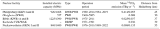
Table 1Nuclear facilities in the surroundings of Heidelberg. Reactor type (BWR: boiling water reactor, PWR: pressurized water reactor), installed electrical power, and the average annual 14CO2 emissions during their respective periods of operation up to 2014, as well as the distance to the Heidelberg sampling site are given. Different reactor blocks are separated by a slash. RR are research reactors and RP is the research reprocessing plant (WAK) of the Karlsruhe Research Center (FZK). After the operation period, further emissions occur during the decommissioning of the facilities (data taken from BfS 1986—2015).
Here we present results from HYSPLIT dispersion modelling (Draxler and Hess, 1998) of 14CO2 emissions from five nuclear installations in the less than 60 km neighbourhood of our long-term Δ14CO2 monitoring site in Heidelberg. We apply the HYSPLIT model for the period of 1986–2014 with available wind fields of 2.5∘ × 2.5∘, 1∘ × 1∘, and 0.5∘ × 0.5∘ resolution. Using reported 14CO2 emission rates, these model estimates for the Heidelberg sampling site allow us to correct for the local 14CO2 contaminations from nuclear facilities (Kuderer, 2016). Our model results, however, turn out to strongly depend on the resolution of the wind field used for the calculation. We discuss this important finding and present the currently most reliable corrections of our long-term Δ14CO2 measurements.
2.1 Site description
The Heidelberg monitoring site is located on the university campus in the outskirts of Heidelberg, a medium sized city in the Upper Rhine valley in southwestern Germany (49∘25′ N, 8∘41′ E, 116 m a.s.l., see Fig. 1). From 1986–2001, CO2 samples for Δ14C analysis have been collected from the roof of the former building of the Institut für Umweltphysik (INF 366), and from 2001 to present from the new building about 500 m to the east (INF 229). At both locations, air was sampled from about 25–30 m a.g.l. The small difference in location of the two sampling sites is not relevant when estimating the nuclear 14CO2 contamination with HYSPLIT.
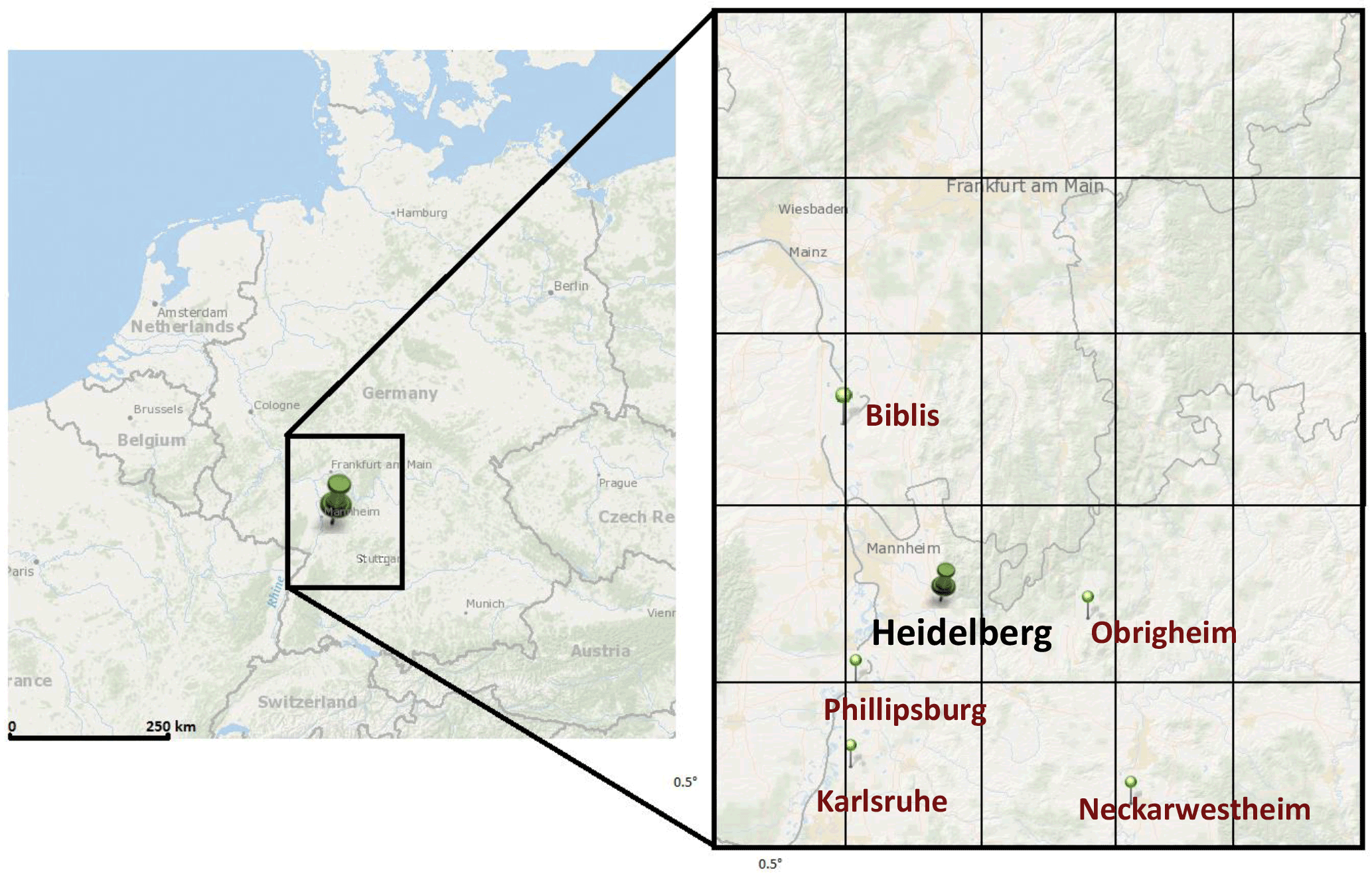
Figure 1Map of the Heidelberg sampling site in southwest Germany. The locations of the five nearest nuclear facilities are shown in the enlargement. This enlargement corresponds to the size of the 2.5∘ × 2.5∘ wind field grid. The 0.5∘ × 0.5∘ wind field resolution is indicated by the grid in the enlargement.
Five nuclear installations with reported 14CO2 emissions are found at distances between 25 and 55 km from the Heidelberg station. Figure 1 shows their locations; details of reactor type, installed electrical output, period of operation, distance from the Heidelberg station, and mean reported 14CO2 emission during their operation up to 2014 are listed in Table 1. As the prevailing winds in the Upper Rhine valley are from the southwest, Philippsburg (KKP I and II) is the most important source of potential 14CO2 contamination in Heidelberg. Philippsburg I is the only boiling water reactor (BWR) with its major 14C emissions being 14CO2, whereas pressurized water reactors (PWR) emit 14C mainly as 14CH4 (Kunz, 1985). All other nuclear installations except for Neckarwestheim II (GKN II) emit less than 15 % of Philippsburg I. Neckarwestheim, however, is located to the southeast of Heidelberg in the Neckar valley at a distance of 55 km, so that its relative contribution to the total 14CO2 contamination is only less than 10 % (see Table 3).
2.2 14CO2 sampling and analysis
Two-week and, for limited periods, also one-week integrated large-volume samples of atmospheric CO2 were collected from the roof of the institute's buildings by quantitative chemical absorption in basic sodium hydroxide (NaOH) solution, as described by Levin et al. (1980). Except for the first few years, samples were collected only during the night (from 19:00 to 07:00 CET, Central European Time) in order to avoid CO2 contamination from local traffic. Moving the institute to a new building in the year 2000 required parallel CO2 sampling at both the old and the new sampling locations on the Heidelberg University campus, in order to quantify possible differences and then allow combining the data sets from the two locations about 500 m apart. As the new building is located closer to the Heidelberg city centre, slightly lower Δ14C values (on average by 0.8 ‰) were found at the new location over the more than 1-year overlapping period from late 2000 to early 2002. The results obtained from samples collected until 2002 at INF 366 at about 25 m a.g.l. were adjusted accordingly, and are now comparable with those obtained at the current sampling location at INF 229 at about 30 m a.g.l. (for details of this comparison and correction, see Levin et al., 2008).
14CO2 samples were processed in the Heidelberg 14C laboratory by acidification of the NaOH solution in a vacuum system. The extracted CO2 was subsequently purified over charcoal. The 14C∕C ratio was then measured by low-level counting (Kromer and Münnich, 1992). All results are presented here as 13C-corrected Δ14C deviations from the international reference standard (oxalic acid) in per mill. They are corrected for decay to the date of CO2 sampling (Stuiver and Polach, 1977). Note that Stuiver and Polach (1977) refer to this 14C notation as Δ not Δ14C; however, in order to be consistent with other atmospheric radiocarbon literature we stick to using Δ14C instead of Δ. The precision of Δ14C values was of the order of 4–5 ‰ in the 1980s and 1990s, 3–4 ‰ in the 2000s, and 2–3 ‰ thereafter.
2.3 Reported 14CO2 emissions from nuclear facilities in the surroundings of Heidelberg
According to the German Atomic Energy Act (Strahlenschutzverordnung, 2001), emissions of radioactive substances from nuclear facilities with the exhaust air must be monitored and reported quarterly to regional and federal authorities. The Bundesamt für Strahlenschutz (BfS, German Federal Office for Radiation Protection), releases yearly reports on radioactive emissions from all German reactors and research facilities; here the 14CO2 emissions are reported separately from other radioactive substances. These BfS reports are available for the years 1986–2014 (BfS, 1986–2015). For Philippsburg I and II higher resolution, i.e. monthly, emission data are available (Kernkraftwerk Philippsburg, personal communication, 2013); these monthly data were used in this work to estimate the 14CO2 contamination in Heidelberg.
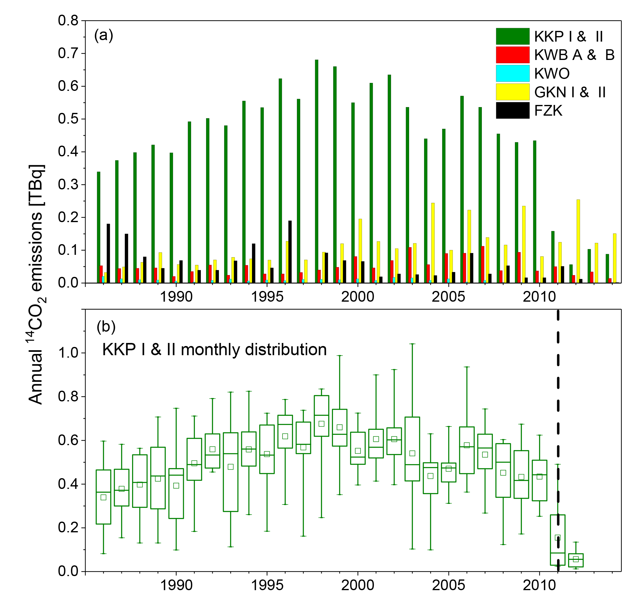
Figure 214CO2 emissions from nuclear facilities: annual mean emissions from all facilities (a) and box plots of the distribution of monthly values from Philippsburg (KKP I and II, b); the boxes include 50 % of all months of the year with the horizontal bar indicating the mean and the square indicating the median value of the year. The whiskers show the minimum and maximum monthly values of the individual years. The dashed line indicates the shutdown of Philippsburg I shortly after the Fukushima accident.
Figure 2a shows annual 14CO2 emissions from 1986–2014 for all five facilities listed in Table 1, while Fig. 2b shows the distribution of monthly emissions from Philippsburg I and II for the years 1986–2012. Note the huge variability in monthly emissions, which can differ from month to month by more than a factor of 2. No seasonal variation nor any relation to particular maintenance activities was observed. Graven and Gruber (2011) estimated mean emission factors of 0.06 TBq 14CO2 GWa−1 for PWRs and 0.51 TBq 14CO2 GWa−1 for BWRs. However, from our emission data and corresponding power production reports, we do see large differences from these emission factors and for PWRs no correlation at all, as displayed in Fig. 3. Moreover, keeping in mind the huge month-to-month variability in 14CO2 emissions from Philippsburg (Fig. 2b), this underlines the necessity for reliable high-resolution 14CO2 emission data from nuclear installations if accurate corrections shall be applied to atmospheric Δ14CO2 observations for fossil fuel CO2 estimates.
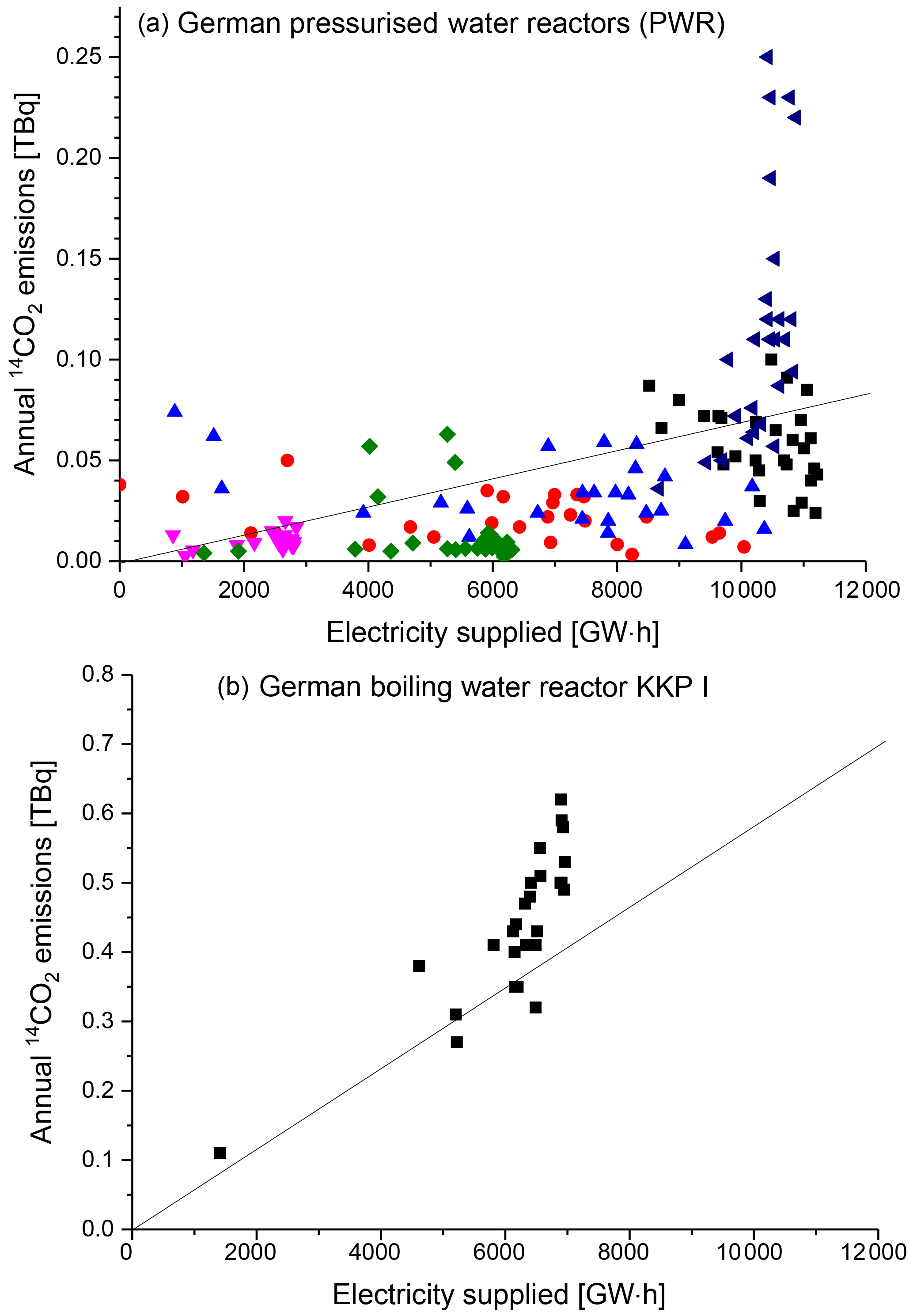
Figure 3Relationship between annual 14CO2 emissions from Pressurized Water Reactors (a) and the Boiling Water Reactor Philippsburg I (b) and their annual electricity supplied. The solid lines show the specific emission factors reported by Graven and Gruber (2011).
2.4 The HYSPLIT model
The Hybrid Single-Particle Lagrangian Integrated Trajectory model (HYSPLIT) from NOAA offers a variety of services ranging from computing simple air parcel trajectories up to complex dispersion simulations (Draxler and Hess, 1998). During the simulations, virtual particles are emitted at the source location and advected to the new particle position, described by the position vector P, using the input wind velocity vector field V:
The advection equation is solved with a dynamic time step Δt, demanding that the advective displacement is smaller than the size of a grid cell (Draxler, 1999). Equation (1) is solved numerically by integrating the velocity vector over time, making use of the trapezoidal rule, i.e. averaging the velocity vectors at the initial position V(P,t) and first-guess position , of the particle. To account for atmospheric dispersion, the particles are displaced stochastically (Eqs. 2a and b):
and
where the turbulent velocity components U′ and W′ are estimated from the standard deviations σ of the horizontal or respective vertical velocity components (Fay et al., 1995). For more details, see Stein et al. (2015) and references therein.
The HYSPLIT model was run here in the forward mode with an internal spatial resolution of 0.05∘ × 0.05∘ and an internal time step fixed by the stability ratio 0.75, i.e. the time step is chosen such that the maximal advective displacement is smaller than 0.75 times the grid size. For every nuclear facility location, a separate run has been conducted with a constant emission rate. Due to the small distance between 14C sources and the measurement station Heidelberg, simulations were limited to 48 h, where each run consisted of a 24 h period, with 2500 particles being emitted every hour, followed by 24 h of sole propagation of the particles. Thus, for each day, the simulated nuclear 14C activity included the actual emissions of this day arriving at the sampling site and the propagated emissions from the day before. This could potentially lead to loss of particles, which arrive at the measurement site more than 24–48 h after the release; but for an extended reference period, only a minor effect has been observed. Note that typical travel times from the nuclear power plants to Heidelberg are of the order of 6–12 h. The HYSPLIT model computes for every hour the particle concentration in every grid box, which gives a dilution factor f (see Eq. 3), describing how much the point source emissions are diluted over the respective grid. This dilution factor is strongly depending on the prevailing meteorological conditions. All relevant control parameters of the different runs are listed in Table 2.
Table 2Control parameters of the HYSPLIT runs and used wind field data for 14CO2 contamination estimates for the different nuclear facilities.
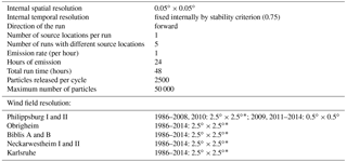
* The HYSPLIT results obtained with 2.5∘ × 2.5∘ wind fields have been corrected with a factor of 0.43
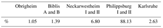
Table 3Relative average Δ14Cnuclear contribution in Heidelberg from 1986 to spring 2011 (shutdown of Philippsburg I).
2.5 Wind fields
Previous studies have shown that HYSPLIT calculations are sensitive to the meteorological input data (e.g. Cabello et al., 2008; Lin et al., 2015). Here we used three different wind velocity fields that have a horizontal resolution of 2.5∘ × 2.5∘, 1∘ × 1∘, and 0.5∘ × 0.5∘. The GDAS (Global Data Assimilation System) assimilates meteorological observations in numerical weather prediction models and archives the results. The one degree fields (GDAS1) are available since 2005 and the half degree fields (GDAS0p5) since 2008. GDAS1 and GDAS0p5 also differ, besides the horizontal, in the vertical resolution (Lin et al., 2015). The NCEP/NCAR (National Centers for Environmental Prediction/National Center for Atmospheric Research) reanalysis provides atmospheric analyses with a spatial resolution of 2.5∘ × 2.5∘, using historical data from 1948 onwards. All three wind fields are readily available at ftp://arlftp.arlhq.noaa.gov/pub/archives/, last access: 29 March 2016.
2.6 Estimation of Δ14Cnuclear
The 14C signal at the sampling site (Δ14Cnuclear) originating from 14CO2 emissions from each nuclear facility is calculated by scaling the meteorological dilution factor f (s m−3) at the measurement station obtained from the HYSPLIT simulation with the time-varying emission strength Q (Bq s−1) of the source. This specific 14C activity is converted (according to its definition from Stuiver and Polach, 1977) into Δ14Cnuclear in per mill according to Eq. (3)
with the molar volume at standard atmospheric temperature and pressure (STP) Vm=24.465 mole m−3, molar mass of carbon MC=12 g mole−1, mole fraction of CO2, , and specific activity of the 14C standard a=0.238 Bq gC−1.
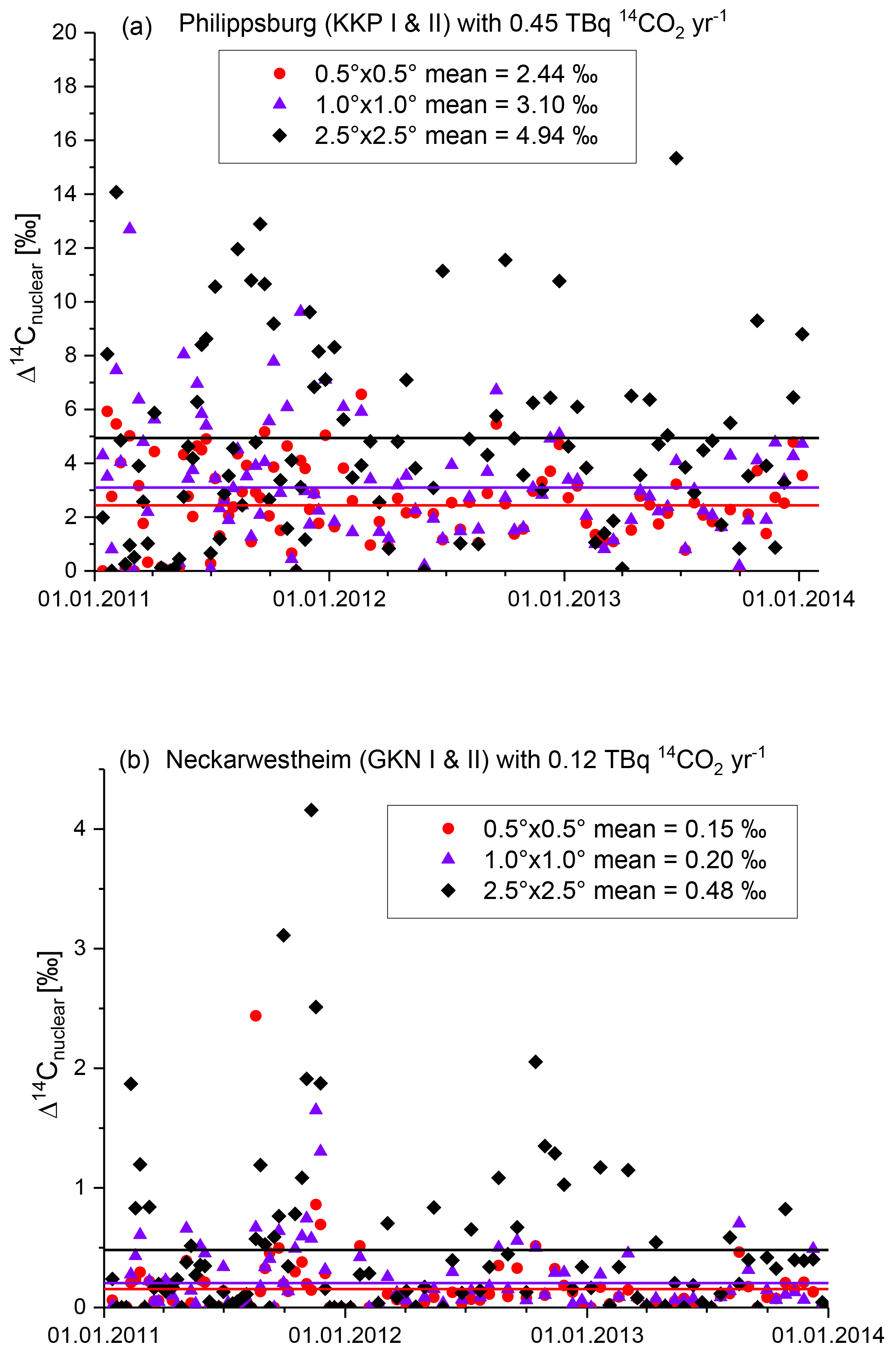
Figure 4(a) Calculated Δ14Cnuclear contributions from Philippsburg with assumed constant 14CO2 emissions using the three wind fields with different resolution. (b) Same as (a), showing the contributions from Neckarwestheim.
3.1 Δ14Cnuclear estimates using wind fields of different resolutions
Figure 4a shows 2-weekly (i.e. sampling period) integrated HYSPLIT-estimated Δ14Cnuclear contributions in Heidelberg for 2011–2013, originating from assumed constant 14CO2 emissions from Philippsburg of 0.45 TBq yr−1 (corresponding to the long-term average emission from this facility). The different symbols distinguish the results when using the three different wind fields, i.e. with resolution of 2.5∘ × 2.5∘ (black diamonds), 1∘ × 1∘ (blue triangles), and the highest resolution of 0.5∘ × 0.5∘ (red circles). The 2-week integrated Δ14Cnuclear signals vary between 0 and 16 ‰ for the coarse resolution wind field, and show on average lower signals when using the higher resolved wind fields. There are, however, also situations when we obtain lower contamination signals with the coarse resolution wind field than with the higher resolved fields. The 1∘ × 1∘ wind field also yields, on average, slightly higher Δ14Cnuclear signals from Philippsburg than the highest resolution (0.5∘ × 0.5∘) wind field, but the differences between those two are often only marginal. Looking at the contributions from the Neckarwestheim reactors (GKN I and II; Fig. 4b), we also estimate the largest Δ14Cnuclear signals with the low-resolution wind field, while the highest resolution wind field yields the smallest signals. The mean ratio between the contamination signals estimated with the highest resolution wind field and those estimated with the 2.5∘ × 2.5∘ resolution field is 0.43. We consider the results from the higher resolution wind fields more reliable to calculate Δ14Cnuclear than those with the coarse resolution field (see discussion below). We can further see that the contributions from Neckarwestheim 14CO2 emissions on the Heidelberg Δ14CO2 signal are, on average, about 1 order of magnitude smaller than those from Philippsburg and, thus, with an average Δ14Cnuclear of less than 0.2 ‰, almost negligible.
3.2 Estimation of Δ14Cnuclear in Heidelberg from all five nuclear installations
Owing to its source strength and proximity to Heidelberg, Philippsburg I is the dominant contributor to the nuclear contamination at our sampling site. Therefore, and considering the high month-to-month variability in emissions (Fig. 2b), it is important to use monthly-resolved emission data to estimate the Δ14Cnuclear signals originating from this facility. The other four nuclear installations are secondary contributors permitting the use of annual average 14CO2 emission rates in absence of higher temporally resolved emission data. For each source location, the HYSPLIT model was run for every calendar day separately covering the period 1986–2014.
For the Philippsburg reactor site, the following meteorological data has been used (Table 2): For 1986–2008 and 2010, we used the 2.5∘ × 2.5∘ fields, for 2009 and 2011–2014 the 0.5∘ × 0.5∘ fields. For the other four source locations (Obrigheim, Biblis A and B, Neckarwestheim 1 and 2, and Karlsruhe), the 2.5∘ × 2.5∘ wind field data have been used for the entire period 1986–2014 in order to save computing time. All coarse grid dilution factors were then corrected with a factor of 0.43 as an attempt to account for the effect of underestimating atmospheric dispersion in coarse grid simulations. This factor was obtained from the comparison made for the 3-year period 2011–2013 at Philippsburg and Neckarwestheim (Fig. 4). The average relative contributions to the total Δ14Cnuclear signal for all facilities are listed in Table 3. The largest correction terms for a 2-week sampling period originating from Philippsburg I and II were 15.2 ‰, from Neckarwestheim I and II it was 3.3 ‰, and from Biblis A and B it was 1.1 ‰. From the other two facilities, they were always smaller than 1 ‰.
The individual uncorrected Heidelberg Δ14CO2 data are displayed in Fig. 5a together with the individual total Δ14Cnuclear corrections Fig. 5b. In the years before the Philippsburg I shutdown, about 1 % of all corrections were above 10 ‰ and less than 2 % above 5 ‰. The mean correction was 2.3 ‰ with a standard deviation of 2.1 ‰. After the shutdown of the BWR Philippsburg I, the largest 14CO2 source before 2011, Δ14Cnuclear decreased to less than 2 ‰, with a mean value of 0.44 ± 0.32 ‰ from 2012 to 2014. It is therefore feasible to only apply an average correction of this size to the Heidelberg measurements of all subsequent years.
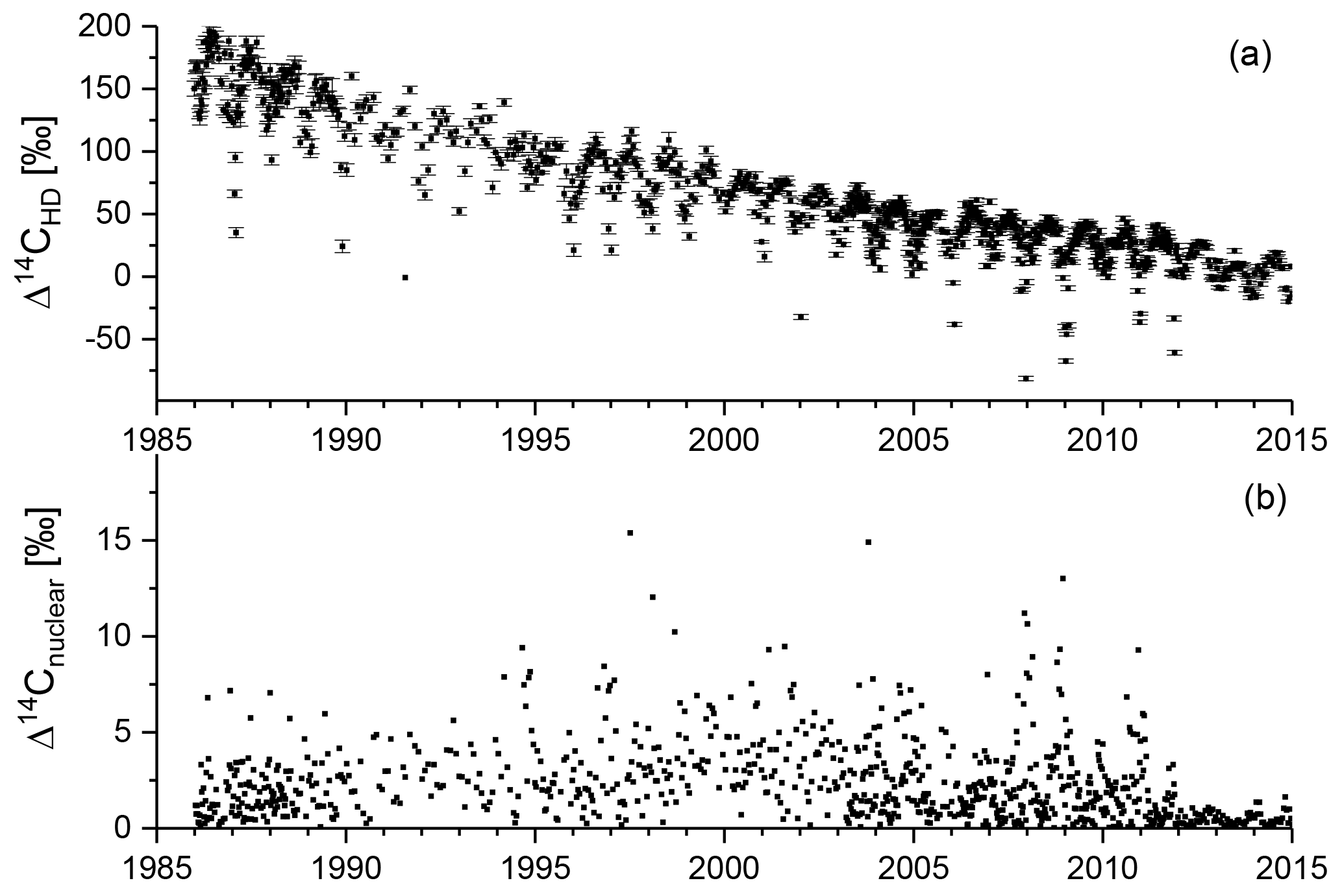
Figure 5(a) Results of Δ14CO2 measurements in Heidelberg (uncorrected); (b) nuclear contribution from all installations in Heidelberg (note expanded Δ14C scale).
3.3 Uncertainty in estimated Δ14Cnuclear
The uncertainty in our Δ14Cnuclear estimates originates from uncertainties in emission data and uncertainties in the HYSPLIT model transport. From comparison with results based on the differently resolved wind fields (Fig. 4), we find the largest deviations between the 2.5∘ × 2.5∘ and the 1∘ × 1∘ fields while the average differences between the two finer resolved wind fields are of the order of 30 %, they can, however, be as large as a factor of 2 for individual 2-week periods. The uncertainty in the measured monthly emission data is probably less than 10–20 % and thus small if compared to the uncertainty in the model transport (although sub-monthly variability in the emissions may also contribute to the uncertainty in the Δ14Cnuclear estimates). For the contributions from nuclear installations where only annual average emission data were available to us, the uncertainty in emissions is estimated to be 30 %. As the contribution from all four installations except Philippsburg contribute on average only 12 % (Table 3), this uncertainty is small compared to the transport uncertainty in the contributions from Philippsburg. We, therefore, estimate the typical uncertainty in individual total Δ14Cnuclear signals to be less than 35 %. It is worth noting from Fig. 4a and b that the variability of Δ14Cnuclear is larger for the 2.5∘ × 2.5∘ wind field calculations than would be expected from the mean differences between the fine and the coarse resolution wind field simulations. Therefore, applying a simple correction factor of 0.43 on all values estimated for the years 1986–2008 and 2010 with the 2.5∘ × 2.5∘ wind field adds variability and uncertainty to the Δ14Cnuclear corrections, which is, however, not possible to quantify with the currently available information.
Our HYSPLIT estimates of 14CO2 contaminations from nuclear facilities in the catchment area of Heidelberg showed large differences when using wind fields of different resolution. The calculated mean contamination was approximately twice as large when using the coarse resolution 2.5∘ × 2.5∘ wind field compared to the two higher resolution fields. Previous studies have shown that meteorological coarse grid reanalyses can be well suited to capture synoptic-scale dynamical processes, but biases in surface wind speeds may be introduced as reanalysis data are not well adapted to reproduce transient strong wind events occurring at the mesoscale and generating a large sub-grid scale variability (Largeron et al., 2015). These can arise in HYSPLIT trajectory calculations, which are the basis for concentration simulations, when the air mass passes through areas with complicated topography and meteorological patterns that are on a smaller scale than the data resolution (Su et al., 2015). Another and possibly more important factor is that atmospheric dispersion is included in the model by using the standard deviation of the interpolated velocity field. Linearly interpolating the coarse wind field to the internal HYSPLIT grid (here 0.05∘ × 0.05∘) leads to a less variable velocity field compared to initially starting with a fine grid. This generates more distinct plume shapes in coarse grid simulations (Kuderer, 2016). Therefore, using the coarse wind field may underestimate the effect of atmospheric dispersion, leading to high values when the plume directly passes the measurement point. We expect this to occur frequently in the case of the Philippsburg 14CO2 plume, where the source lies in the main wind direction at rather short distance from the measurement point. This effect may explain the occasionally high Δ14Cnuclear values estimated for a number of sampling periods before 2009 (Fig. 5b), which are not seen in the measured uncorrected data (Fig. 5a). In the case of Neckarwestheim, this explanation does not hold. However, here we also consider the results obtained with the finest resolution wind field as more accurate. Neckarwestheim lies in the hilly Neckar valley with a complex topography, which is probably better represented by the finer resolution wind fields. Overall, we expect the HYSPLIT estimates that are based on higher resolution wind fields to provide more realistic results, in particular as the topography around Heidelberg is not flat. We therefore correct the HYSPLIT results obtained with the 2.5∘ × 2.5∘ wind fields for the earlier years when high-resolution wind fields (0.5∘ × 0.5∘) are not available. Note, however, that this first rough correction comes with additional uncertainty and variability (see above).
In an earlier study by Levin et al. (2003), Philippsburg I and II were considered as the sole sources for the nuclear contamination at the Heidelberg sampling site. A Gaussian plume model (Turner, 1970) with a constant mean dispersion factor had been applied there to calculate Δ14Cnuclear as a first approximation, but using the same monthly 14CO2 emissions as in the present study. The mean nuclear signal estimated by Levin et al. (2003) was Δ14Cnuclear ‰ ranging from 0.2 to 10 ‰ for monthly mean values. This earlier estimate of 14CO2 contamination is approximately twice the value obtained with the HYSPLIT model and the high-resolution wind fields. Graven and Gruber (2011) used the TM3 model with a spatial resolution of 1.8∘ × 1.8∘ and estimated for 2005 a total Δ14Cnuclear of 2.1 (1.1–3.7) ‰ for the Heidelberg grid cell. Their estimate is in agreement with our results for that year (2.1 ± 1.6 ‰) obtained with the 2.5∘ × 2.5∘ resolution wind field corrected by the factor of 0.43. As in the present study, Graven and Gruber (2011) also included 14C contributions from other nuclear installations in their estimates. However, their assumed emissions from the Philippsburg I reactor were estimated with the average emission factor for BWR, which is about 20 % smaller than the measured value for 2005 used in our estimate. They also mention that their Eulerian model may have underestimated the true contamination due to its coarse resolution, which would dilute point source emissions over a large grid in an Eulerian approach.
These comparisons with earlier studies indicate that more work and higher resolution models and wind fields are needed to reduce the uncertainty in the 14CO2 contamination estimates from nuclear installations at measurement sites where Δ14CO2 observations shall be used to precisely determine the regional fossil fuel CO2 component. Currently, we have to take into account a model transport uncertainty of about 1–2 ‰ in the estimated Δ14Cnuclear contamination, if the measurement site is located closer than about 30 km downwind from a nuclear facility, which has a 14CO2 emission rate of about 0.5 TBq yr−1 similar to the Philippsburg I boiling water reactor with 1 MWe power production. Other reactor types, such as the Canadian CANDU reactors may have significantly larger emission rates (Graven and Gruber, 2011; Vogel et al., 2013); the uncertainty in corresponding Δ14Cnuclear estimates in their close neighbourhood may then be considerably larger.
The limited temporal resolution of 14CO2 emission rates from nuclear installations cause additional uncertainty in the Δ14Cnuclear estimates, as generally only annual mean emissions are reported. Graven and Gruber (2011) assume that 14CO2 emissions are proportional to the annual power production. However, the present study on the influence from German reactors on the Heidelberg measurement site does not fully support this finding. Figure 3 does not show significant correlations between annual 14CO2 emissions and corresponding electricity supply. Therefore, assuming emission factors as suggested by Graven and Gruber (2011) will add considerable uncertainty to the Δ14Cnuclear estimates, which may be as large as the uncertainties estimated here for the wind-field-based model transport error.
Overall, we conclude that careful investigation of potential 14CO2 emissions in the catchment of sampling sites is required when using Δ14CO2 observations for fossil fuel CO2 estimates. The differences in our HYSPLIT modelling results, when based on differently resolved wind fields together with the findings from earlier studies, suggest that current Δ14Cnuclear estimates may be wrong by a factor of 2. Therefore, careful investigations with high-resolution models must be performed at all stations where 14C-based fossil fuel CO2 measurements are conducted. Based on our simulations, the shutdown of Philippsburg I in 2011, if not accounted for in the Δ14Cnuclear correction, would have masked a fossil fuel CO2 signal of 1 ppm, corresponding to 10 % of the average total fossil fuel CO2 signal in Heidelberg. Therefore, we plan similar studies for the European ICOS atmospheric station network (https://www.icos-ri.eu/icos-stations-network, last access: 5 June 2018). The basis must be high-resolution 14CO2 emissions data from nuclear facilities, which need to be made available for these investigations if contamination estimates are to be accurate.
Data will be available from the Heidelberg University data depository under https://heidata.uni-heidelberg.de/dataverse/carbon (https://doi.org/10.11588/data/RYRDZQ).
IL and SH have designed the study. MK made the HYSPLIT model calculations and evaluated the data. IL prepared the manuscript with support from MK and SH.
The authors declare that they have no conflict of interest.
The authors gratefully acknowledge the NOAA Air Resources Laboratory (ARL)
for providing the HYSPLIT transport and dispersion model used in this
publication. We would especially like to thank Bernd Kromer and the staff of the
Heidelberg 14C laboratory for their careful work analysing the
14CO2 samples, and Ute Karstens for helpful discussions on the
manuscript. Financial support came from a number of agencies in Germany and
Europe. These are the Heidelberg Academy of Sciences, the German Ministries
for the Environment, Education and Science, and Transportation and
Digital Infrastructure, as well as the German Umweltbundesamt and the European
Commission, Brussels. We acknowledge financial support by Deutsche
Forschungsgemeinschaft within the funding programme Open Access Publishing,
by the Baden-Württemberg Ministry of Science, Research and the Arts, and
by Ruprecht-Karls-Universität Heidelberg.
Edited by: Thomas Röckmann
Reviewed by: Jocelyn Turnbull
and one anonymous referee
BfS: Umweltradioaktivität und Strahlenbelastung: Jahresberichte, Bundesamt für Strahlenschutz (BfS), Bundesministerium für Umwelt, Naturschutz, Bau und Reaktorsicherheit (BMBU), available at: http://nbn-resolving.de/urn:nbn:de:0221-2017072814305 (last access: 20 March 2016), 1986–2015.
Cabello, M., Orza, J. A. G., Galiano, V., and Ruiz, G.: Influence of meteorological input data on backtrajectory cluster analysis – a seven-year study for southeastern Spain, Adv. Sci. Res., 2, 65–70, https://doi.org/10.5194/asr-2-65-2008, 2008.
Draxler, R.: HYSPLIT4 user's guide. Technical report, NOAA ARL. NOAA Air Resources Laboratory, Silver Spring, MD, 1999.
Draxler, R. R. and Hess, G. D.: An Overview of the HYSPLIT_4 modeling system for trajectories, dispersion and deposition, Aust. Met. Mag., 47, 295–308, 1998.
Fay, B., Glaab, H., Jacobsen, I., and Schrodin, R.: Evaluation of Eulerian and Lagrangian atmospheric transport models at the Deutscher Wetterdienst using anatex surface tracer data, Atmos. Environ., 29, 2485–2497, 1995.
Graven, H.: Impact of fossil fuel emissions on atmospheric radiocarbon and various applications of radiocarbon over this century, P. Natl. Acad. Sci. USA, 112, 9542–9545, 2015.
Graven, H. D. and Gruber, N.: Continental-scale enrichment of atmospheric 14CO2 from the nuclear power industry: potential impact on the estimation of fossil fuel-derived CO2, Atmos. Chem. Phys., 11, 12339–12349, https://doi.org/10.5194/acp-11-12339-2011, 2011.
Kromer, B. and Münnich, K. O.: CO2 gas proportional counting in Radiocarbon dating – review and perspective, in: Radiocarbon after four decades, edited by: Taylor, R. E., Long, A., and Kra, R. S., Springer-Verlag, New York, 184–197, 1992.
Kuderer, M.: Influence of nuclear power plants to the radiocarbon budget in Heidelberg and trajectory-based sampling, Master-Thesis, Universität Heidelberg, 2016.
Kunz, C.: Carbon-14 discharge at three light-water reactors, Health Phys., 49, 25–35, 1985.
Largeron, Y., Guichard, F., Bouniol, D., Couvreux, F., Kergoat, L., and Marticorena, B.: Can we use surface wind fields from meteorological reanalyses for Sahelian dust emission simulations?, Geophys. Res. Lett., 42, 2490–2499, 2015.
Levin, I. and Hesshaimer, V.: Radiocarbon – a unique tracer of global carbon cycle dynamics, Radiocarbon, 42, 69–80, 2000.
Levin, I., Münnich, K. O., and Weiss, W.: The effect of anthropogenic CO2 and 14C sources on the distribution of 14CO2 in the atmosphere, Radiocarbon, 22, 379–391, 1980.
Levin, I., Kromer, B., Barabas, M., and Münnich, K. O.: Environmental distribution and long-term dispersion of reactor 14CO2 around two German nuclear power plants, Health Phys., 54, 149–156, 1988.
Levin, I., Bösinger, R., Bonani, G., Francey, R. J., Kromer, B., Münnich, K. O., Suter, M., Trivett, N. B. A., and Wölfli, W.: Radiocarbon in atmospheric carbon dioxide and methane: global distribution and trends, in: Radiocarbon After Four Decades: An Interdisciplinary Perspective, edited by: Taylor, R. E., Long, A., and Kra, R. S., Springer-Verlag, New York, 503–517, 1992.
Levin, I., Kromer, B., Schmidt, M., and Sartorius, H.: A novel approach for independent budgeting of fossil fuels CO2 over Europe by 14CO2 observations, Geophys. Res. Lett., 30, 2194, https://doi.org/10.1029/2003GL018477, 2003.
Levin, I., Hammer, S., Kromer, B., and Meinhardt, F.: Radiocarbon Observations in Atmospheric CO2: Determining Fossil Fuel CO2 over Europe using Jungfraujoch Observations as Background, Sci. Total. Environ., 391, 211–216, https://doi.org/10.1016/j.scitotenv.2007.10.019, 2008.
Levin, I., Naegler, T., Kromer, E., Diehl, M., Francey, R. J., Gomez-Pelaez, A. J., Schäfer, A., Steele, L. P., Wagenbach, D., Weller, R., and Worthy, D. E.: Observations and modelling of the global distribution and long-term trend of atmospheric 14CO2, Tellus, 62B, 26–46, https://doi.org/10.1111/j.1600-0889.2009.00446.x, 2010.
Lin, S., Zibing, Y., Fung, J. C. H., and Lau, A. K. H.: A comparison of HYSPLIT backward trajectories generated from two GDAS datasets, Sci. Total. Environ., 506–507, 527–537, https://doi.org/10.1016/j.scitotenv.2014.11.072, 2015.
Pasquill, F.: The estimation of the dispersion of windborne material, Meteorol. Mag., 90, 1063, 33–49, 1961.
Povinec, P. P., Chudý, M., Šivo, A., Šimon, J., Holý, K., and Richtáriková, M.: Forty years of atmospheric radiocarbon monitoring around Bohunice nuclear power plant, Slovakia, J. Environ. Radioactiv., 100, 125–130, 2009.
Stein, A., Draxler, R., Rolph, G., Stunder, B., Cohen, M., and Ngan, F.: NOAA's hysplit atmospheric transport and dispersion modeling system, B. Am. Meteorol. Soc., 96, 2059–2077, https://doi.org/10.1175/BAMS-D-14-00110.1, 2015.
Strahlenschutzverordnung: § 47, available at: https://www.jurion.de/Gesetze/StrlSchV-1/47 (last access: 29 March 2016), 2001.
Stuiver, M. and Polach, H.: Discussion: Reporting of 14C Data, Radiocarbon, 3, 355–363, 1977.
Su, L., Yuan, Z., Fung, J. C., and Lau, A. K.: A comparison of HYSPLIT backward trajectories generated from two GDAS datasets, Sci. Total Environ., 506–507, 527–537, 2015.
Turnbull, J., Rayner, P., Miller, J., Naegler, T., Ciais, P., and Cozic, A.: On the use of 14CO2 as a tracer for fossil fuel CO2: Quantifying uncertainties using an atmospheric transport model, J. Geophys. Res., 114, D22302, https://doi.org/10.1029/2009JD012308, 2009.
Turner, D. B.: Workbook of atmospheric dispersion estimates, Publication No. AP-26, U.S. Environ. Prot. Agency, Raleigh, 1970.
Uchrin, G., Hertelendi, E., Volent, G., Slavik, O., Morávek, J., Kobal, I., and Vokal, B.: 14C measurements at PWR-type nuclear power plants in three middle European countries, Radiocarbon, 40, 439–446, 1998.
Vogel, F., Levin, I., and Worthy, D. E. J.: Implications of using parameterized nuclear power plant emissions of 14CO2 on deriving reliable estimates of fossil fuel CO2 from atmospheric observations, in: Proceedings of the 21st International Radiocarbon Conference, edited by: Jull, A. J. T. and Hatté, C., Radiocarbon, 55, 1556–1572, 2013.