the Creative Commons Attribution 3.0 License.
the Creative Commons Attribution 3.0 License.
Global soil consumption of atmospheric carbon monoxide: an analysis using a process-based biogeochemistry model
Licheng Liu
Shaoqing Liu
Hella van Asperen
Mari Pihlatie
Carbon monoxide (CO) plays an important role in controlling the oxidizing capacity of the atmosphere by reacting with OH radicals that affect atmospheric methane (CH4) dynamics. We develop a process-based biogeochemistry model to quantify the CO exchange between soils and the atmosphere with a 5 min internal time step at the global scale. The model is parameterized using the CO flux data from the field and laboratory experiments for 11 representative ecosystem types. The model is then extrapolated to global terrestrial ecosystems using monthly climate forcing data. Global soil gross consumption, gross production, and net flux of the atmospheric CO are estimated to be from −197 to −180, 34 to 36, and −163 to −145 Tg CO yr−1 (1 Tg = 1012 g), respectively, when the model is driven with satellite-based atmospheric CO concentration data during 2000–2013. Tropical evergreen forest, savanna and deciduous forest areas are the largest sinks at 123 Tg CO yr−1. The soil CO gross consumption is sensitive to air temperature and atmospheric CO concentration, while the gross production is sensitive to soil organic carbon (SOC) stock and air temperature. By assuming that the spatially distributed atmospheric CO concentrations (∼ 128 ppbv) are not changing over time, the global mean CO net deposition velocity is estimated to be 0.16–0.19 mm s−1 during the 20th century. Under the future climate scenarios, the CO deposition velocity will increase at a rate of 0.0002–0.0013 mm s−1 yr−1 during 2014–2100, reaching 0.20–0.30 mm s−1 by the end of the 21st century, primarily due to the increasing temperature. Areas near the Equator, the eastern US, Europe and eastern Asia will be the largest sinks due to optimum soil moisture and high temperature. The annual global soil net flux of atmospheric CO is primarily controlled by air temperature, soil temperature, SOC and atmospheric CO concentrations, while its monthly variation is mainly determined by air temperature, precipitation, soil temperature and soil moisture.


Carbon monoxide (CO) plays an important role in controlling the oxidizing capacity of the atmosphere by reacting with OH radicals (Logan et al., 1981; Crutzen, 1987; Khalil and Rasmussen, 1990; Prather et al., 1995; Prather and Ehhalt, 2001). CO in the atmosphere can directly and indirectly influence the fate of critical greenhouse gases such as methane (CH4) and ozone (O3) (Tan and Zhuang, 2012). Although CO itself absorbs only a limited amount of infrared radiation from the Earth, the cumulative indirect radiative forcing of CO may be even larger than that of the third powerful greenhouse gas, nitrous oxide (N2O, Myhre et al., 2013). Current estimates of global CO emissions from both anthropogenic and natural sources range from 1550 to 2900 Tg CO yr−1, which are mainly from anthropogenic and natural direct emissions and from the oxidation of methane and other volatile organic compounds (VOCs) (Prather et al., 1995; Khalil et al., 1999; Bergamaschi et al., 2000; Prather and Ehhalt, 2001; Stein et al., 2014). Chemical consumption of CO by atmospheric OH and the biological consumption of CO by soil microbes are two major sinks of the atmospheric CO (Conrad, 1988; Lu and Khalil, 1993; Yonemura et al., 2000; Whalen and Reeburgh, 2001).
Soils are globally considered as a major sink for CO due to microbial activities (Whalen and Reeburgh, 2001; King and Weber, 2007). A diverse group of soil microbes including carboxydotrophs, methanotrophs and nitrifiers are capable of oxidizing CO (King and Weber, 2007). Annually, 10–25 % of total earth surface CO emissions were consumed by soils (Sanhueza et al., 1998; King, 1999a; Chan and Steudler, 2006). Potter et al. (1996) reported the global soil consumption to be from −50 to −16 Tg CO yr−1 (negative values represent the uptake from the atmosphere to soil), by using a single-box model over the upper 5 cm of soils. All existing estimates have large uncertainties and range from −640 to −16 Tg CO yr−1 (Sanhueza et al., 1998; King, 1999b; Bergamaschi et al., 2000). Similarly, the estimates of CO dry deposition velocities also have large uncertainties and range from 0 to 4.0 mm s−1; here, positive values represent deposition to soils (King, 1999a; Castellanos et al., 2011). Soils also produce CO mainly via abiotic processes such as thermal degradation and photo-degradation of organic matter or plant materials (Conrad and Seiler, 1985; Tarr et al., 1995; Schade and Crutzen, 1999; Derendorp et al., 2011; Lee et al., 2012; van Asperen et al., 2015; Fraser et al., 2015; Pihlatie et al., 2016), except for a few cases of anaerobic formation. Photo-degradation is identified as radiation-dependent degradation due to absorbing radiation (King et al., 2012). Thermal degradation is identified as the temperature-dependent degradation of carbon in the absence of radiation and possibly oxygen (Derendorp et al., 2011; Lee et al., 2012; van Asperen et al., 2015; Pihlatie et al., 2016). These major soil CO production processes, together with soil CO consumption processes, have not been adequately considered in global soil CO budget estimates.
To date, most top–down atmospheric models have applied a dry deposition scheme based on the resistance model of Wesely (1989). Such schemes provided a wide range of dry deposition velocities (Stevenson et al., 2006). Only a few models (MOZART-4, Emmons et al., 2010; CAM-chem, Lamarque et al., 2012) have extended their dry deposition schemes with a parameterization for CO and H2 uptake through oxidation by soil microbes, following the work of Sanderson et al. (2003), which was based on extensive measurements from Yonemura et al. (2000). Potter et al. (1996) developed a bottom–up model to simulate CO consumption and production at the global scale. Their model is a single-box model that only considers the top 5 cm depth of soil and does not have explicit microbial factors, and therefore might have underestimated CO consumption (Potter et al., 1996; King, 1999a). Current bottom–up CO modeling approaches are mostly based on a limited number of CO in situ observations or laboratory studies to quantify regional and global soil consumption (Potter et al., 1996; Sanhueza et al., 1998; Khalil et al., 1999; King, 1999a; Bergamaschi et al., 2000; Prather and Ehhalt, 2001). To our knowledge, no detailed process-based model of soil–atmospheric exchange of CO has been published in the last 15 years. One reason is that there is an incomplete understanding of biological processes of uptake (King and Weber, 2007; Vreman et al., 2011; He and He, 2014; Pihlatie et al., 2016). Another reason is that there is a lack of long-term CO flux measurements for different ecosystem types to calibrate and evaluate the models. CO flux measurements are mostly from short-term field observations or laboratory experiments (e.g., Conrad and Seiler, 1985; Funk et al., 1994; Tarr et al., 1995; Zepp et al., 1997; Kuhlbusch et al., 1998; Moxley and Smith, 1998; Schade et al., 1999; King and Crosby, 2002; Varella et al., 2004; Lee et al., 2012; Bruhn et al., 2013; van Asperen et al., 2015). The first study to report long-term and continuous field measurements of CO flux over grasslands using a micrometeorological eddy covariance (EC) method is Pihlatie et al. (2016).
To improve the quantification of the global soil CO budget for the period 2000–2013 and the CO deposition velocity for the 20th and 21st centuries, this study developed a CO dynamics module (CODM) embedded in a process-based biogeochemistry model, the Terrestrial Ecosystem Model (TEM) (Zhuang et al., 2003, 2004, 2007). The CODM was then calibrated and evaluated using laboratory experiments and field measurements for different ecosystem types. The atmospheric CO concentration data from MOPITT (Gille, 2013) were used to drive model simulations from 2000 to 2013. A set of century-long simulations of 1901–2100 were also conducted using the atmospheric CO concentrations estimated with an empirical function (Badr and Probert, 1994; Potter et al., 1996). Finally, the effects of multiple forcings on the global CO consumption and production, including the changes in climate and atmospheric CO concentrations at the global scale, were evaluated with the model.
2.1 Overview
We first developed a soil CO dynamics module (CODM) on a daily time step that considers (1) the soil–atmosphere CO exchange and diffusion process between soil layers, (2) the consumption by soil microbial oxidation, (3) the production by soil chemical oxidation, and (4) the effects of temperature, soil moisture, soil CO substrate and surface atmospheric CO concentration on these processes. Second, we used the observed soil temperature and moisture to evaluate the TEM hydrology module and the soil thermal module in order to estimate soil physical variables. Then we used the data from laboratory experiments and CO flux measurements to parameterize the model using the Shuffled Complex Evolution (SCE-UA) method (Duan et al., 1993). Finally, the model was extrapolated to the globe at a 0.5∘ by 0.5∘ resolution. We conducted three sets of model experiments to investigate the impact of climate and atmospheric CO concentrations on soil CO dynamics: (1) simulations for 2000–2013 with MOPITT satellite atmospheric CO concentration data; (2) simulations for 1901–2100 with constant atmospheric CO concentrations estimated from an empirical function and the historical climate data (1901–2013) and three future climate scenarios (2014–2100); and (3) eight sensitivity simulations by increasing and decreasing (a) constant CO surface concentrations by 30 %, (b) SOC by 5 %, (c) precipitation by 20 % and (d) air temperature by 3∘C for each pixel, respectively, while holding other forcing data as they were, during 1999–2000.
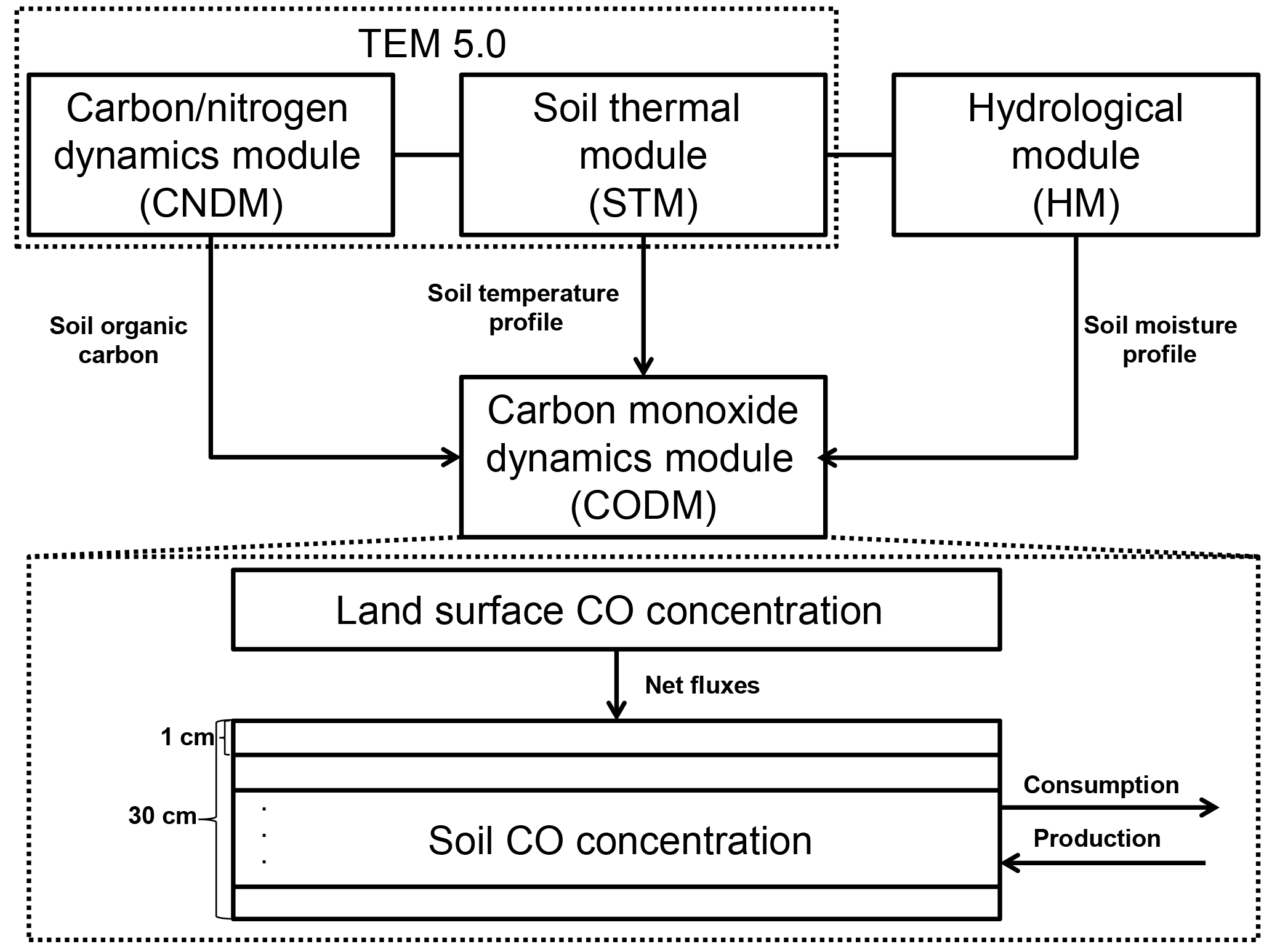
Figure 1The model framework includes a carbon and nitrogen dynamics module (CNDM), a soil thermal module (STM) from Terrestrial Ecosystem Model (TEM) 5.0 (Zhuang et al., 2001, 2003), a hydrological module (HM) based on a land surface module (Bonan, 1996; Zhuang et al., 2004), and a carbon monoxide dynamics module (CODM). The detailed structure of CODM includes land surface CO concentration as the top boundary and 30 1 cm thick layers (in total, 30 cm) where consumption and production take place.
2.2 Carbon monoxide dynamics module (CODM)
Embedded in the TEM (Fig. 1), the CODM is mainly driven by (1) soil organic carbon availability based on a carbon and nitrogen dynamics module (CNDM) (Zhuang et al., 2003); (2) a soil temperature profile from a soil thermal module (STM) (Zhuang et al., 2001, 2003); and (3) a soil moisture profile from a hydrological module (HM) (Bonan, 1996; Zhuang et al., 2004). The net exchange of CO between the atmosphere and soil is determined by the mass balance approach (net flux = total production – total oxidation – total soil CO concentration change). According to previous studies, we separated active soils (top 30 cm) for CO consumption and production into 1 cm thickness layers (King, 1999a, b; Whalen and Reeburgh, 2001; Chan and Steudler, 2006). Between the soil layers, the changes in CO concentrations were calculated as
where C(ti) is the CO concentration (mg m−3) in layer i and at time t. z is the depth of the soil (m). D(t,i) is the diffusion coefficient (m2 s−1) for layer i. P(t,i) is the CO production rate (mg m−3 s−1) and O(t,i) is the CO consumption rate (mg m−3 s−1). D(t,i) is calculated using the method from Potter et al. (1996), which is a function of soil temperature, soil texture and soil moisture. The upper boundary condition is the atmospheric CO concentration, which is estimated with an empirical function of latitude (Potter et al., 1996) or directly measured by the MOPITT satellite during 2000–2013. The lower boundary condition is assumed to have no diffusion exchange with the layer underneath. This partial differential equation (PDE) is solved using the Crank–Nicolson method for a less time-step-sensitive solution.
The CO consumption was modeled in unsaturated soil pores as
where Vmax is the ecosystem-specific maximum oxidation rate and was estimated previously ranging from 0.3 to 11.1 µg CO g−1 h−1 for different ecosystems (Whalen and Reeburgh, 2001). fi represents the effects of soil CO concentration C(t,i), temperature T(t,i) and moisture M(t,i) on the CO soil consumption. Considering the CO consumption as the result of microbial activities, we calculated f1(C(t,i)), f2(T(t,i)) and f3(M(t,i)) in a similar way to Zhuang et al. (2004):
where f1(C(t,i)) is a multiplier that enhances the oxidation rate with increasing soil CO concentrations using a Michaelis–Menten function with a half-saturation constant kCO, and their values were previously estimated ranging from 5 to 51 µl CO l−1 for different ecosystems (Whalen and Reeburgh, 2001); f2(T(t,i)) is a multiplier that enhances the CO oxidation rate with increasing soil temperature using a Q10 function with Q10 coefficients (Whalen and Reeburgh, 2001). Tref is the reference temperature; units are ∘C (Zhuang et al., 2004, 2013). f3(M(t,i)) is a multiplier to estimate the biological limiting effect that diminishes the CO oxidation rates if the soil moisture is not at an optimum level (Mopt). Mmin, Mmax and Mopt are the minimum, maximum and optimum volumetric soil moisture of oxidation reaction, respectively. Equation (2b) will overestimate the CO consumption at high temperature because in reality the CO consumption will decrease when temperature is higher than optimum temperature, while f2 will keep increasing with rising temperature. However, the CO consumption is constrained by the CO production, and Eq. (1) is used to represent this constraint.
We modeled the CO production rate (P(t,i)) as a process of chemical oxidation constrained by the soil organic carbon (SOC) decay (Conrad and Seiler, 1985; Potter et al., 1996; Jobbagy and Jackson, 2000; van Asperen et al., 2015):
where Pr(t,i) is a reference soil CO production rate which has been normalized to the rate at reference temperature (the production rate at temperature (t,i) divided by the production rate at the reference temperature), which is affected by soil moisture and soil temperature (Conrad and Seiler, 1985; van Asperen et al., 2015). ESOC is an estimated nominal CO production factor of 3.5 ± 0.9 × 10⁻⁹ mg CO m−2 s−1 per g SOC m−2 (to 30 cm soil depth) (Potter et al., 1996). CSOC(t) is a SOC content (mg m−2), which is provided by a CNDM in the TEM. FSOC is a constant fraction of top 30 cm SOC compared to the total amount of SOC, which is 0.33 for shrubland areas, 0.42 for grassland areas and 0.50 for forest areas, respectively (Jobbagy and Jackson, 2000). Pr(t,i) was calculated as
where Eq. (3a) is derived from the Arrhenius equation for chemical reactions and normalized using the reference temperature PTref. Earef∕R is the reference activation energy divided by gas constant R; units are K. f4(M(t,i)) is the multiplier that reduces activation energy using a regression approach based on the laboratory experiment of moisture influences on CO production (Conrad and Seiler, 1985). PMref is the reference volumetric soil moisture, ranging from 0.01 to 0.5 volume volume−1 (v v−1). We assumed the thermal degradation to be the main CO producing process due to a lack of photo-degradation data and it being hard to distinguish photo-degradation from observations. In order to reduce the bias from the thermal degradation to the total abiotic degradation, Eq. (3a) is parameterized by comparing with the total production rate. For instance, Pr(t,i) calculation can perfectly fit the experiment results in Van Asperen et al. (2015) with proper PTref (18 ∘C), Earef∕R (14 000 K), and PMref (0.5 v v−1).
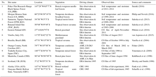
Table 1Model parameterization sites for the thermal and hydrology modules (site nos. 1–4) and for the CODM (site nos. 5–13).
The CO deposition velocity was modeled in the same way as Eq. (19.1) in Seinfeld and Pandis (1998):
where vd is the CO deposition velocity (mm s−1). Fnet is the model estimated CO net flux rate (mg CO m−2 day−1). CCO,air is the CO surface concentration (ppbv). CCO,air can be MOPITT CO surface concentration data or the derived CO surface concentrations using the same method as Potter et al. (1996). Positive values of vd represent soil uptake (deposition from air to soils) and negative values represent soil emissions.

Figure 2Evaluation of thermal and hydrology module at four sites: (a) Boreal evergreen needleleaf forests; (b) temperate deciduous broadleaf forests. (1) shows the soil temperature comparison between the model simulations (gray line) and observations (black line) and (2) shows the soil moisture comparison between the model simulations (gray line) and observations (black line). Specifically, the volumetric soil moisture is converted from the water content reflectometry (WCR) probe output period using an empirical calibration function of Bourgeau-Chavez et al. (2012) for the 5–30 cm layer. Some of them resulted in calculations of values greater than 100 % volumetric soil moisture (VSM) in the Nakai et al. (2013) study. Our model estimated high VSM (close to 80 %) is due to top 10 cm moss in the model, which has a saturation VSM of 0.8. Evaluation of the thermal and hydrology module at four sites: (c) tropical moist forest, (d) tropical forest–savanna. (1) shows the soil temperature comparison between the model simulations (gray line) and observations (black line) and (2) shows the soil moisture comparison between the model simulations (gray line) and observations (black line).
2.3 Model parameterization and extrapolation
The model parameterization was conducted in two steps: (1) thermal and hydrology modules embedded in the TEM were revised, calibrated and evaluated by running a model driven by corresponding local meteorological or climatic data at four representative sites, including boreal forest, temperate forest, tropical forest and savanna (Table 1, site nos. 1 to 4, Fig. 2) to minimize model–data mismatch in terms of soil temperature and moisture. (2) The CODM module was parameterized by running the TEM for observational periods driven with the corresponding local meteorological or climatic data at each reference site (Table 1, Fig. 3), and using the Shuffled Complex Evolution Approach in the R language (SCE-UA-R) (Duan et al., 1993) to minimize the difference between the simulated and observed net CO flux. Eleven parameters including kCO, Vmax, Tref, Q10, Mmin, Mmax, Mopt, ESOC, Earef∕R, PMref and PTref were optimized (Table 2). FSOC was not involved in the calibration process. Parameter priors were decided based on previous studies (Conrad and Seiler, 1985; King, 1999b; Whalen and Reeburgh, 2001; Zhuang et al., 2004). The SCE-UA-R was used for site nos. 6, 8, 10, 11 (Table 1). In parameter ensemble simulations, we have run 50 times SCE-UA-R with 10 000 maximum loops for each site, and all of them have reached a stable state before the end of the loops. For wetlands, the only available data for calibration are from site no. 12. We used the trial-and-error method to make the simulated results in the range of observed flux rates, with a 10 % tolerance. For tropical sites, since the tropical savanna vegetation type is treated as a combination type of tropical forest and grassland in our simulations, we first used site no. 13 to set priors to fit the experiment results with a 10 % tolerance and then evaluated it by running our model and comparing it with the site no. 7 results. Site nos. 9 and 5 were used to evaluate our model results for temperate forest and grassland. Besides the observed climatic and soil property data, we used the ERA-Interim reanalysis data from the European Centre for Medium-Range Weather Forecasts (ECMWF) (Dee et al., 2011), AmeriFlux observed meteorology data (US-Dk3, Novick et al., 2016; CA-Man, Amiro, 2016) and reanalysis climatic data from the Climatic Research Unit (CRU, Harris et al., 2013) to fill the missing environmental data. To sum up, parameters for various ecosystem types in Table 2 were the final results of our parameterization. Model parameterization was conducted for ecosystem types including boreal forest, temperate coniferous forest, temperate deciduous forest, and grassland using SCE-UA-R. In contrast, for tropical forest and wet tundra, we used a trial-and-error method to adjust parameters to allow the model simulation to best fit the observed data. Due to limited data availability, we assumed temperate evergreen broadleaf forests have the same parameters as temperate deciduous forest ecosystems.
Table 2Ecosystem-specific parameters in the CODMa.
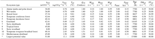
a kCO is the half-saturation constant for soil CO concentration; Vmax is the specific maximum CO oxidation rate; Tref is the reference temperature to account for the soil temperature effects on the CO consumption; Q10 is the ecosystem-specific Q10 coefficient to account for soil temperature effects on the CO consumption; Mmin, Mmax, and Mopt are the minimum, optimum, and maximum volumetric soil moisture of oxidation reaction to account for soil moisture effects on the CO consumption; ESOC is an estimated nominal CO production factor, similar to Potter et al. (1996) (10−4 mg CO m−2 d−1 per g SOC m−2); FSOC is a constant fraction of top 20 cm SOC compared to the total amount of SOC to account for SOC effects on the CO production; Earef∕R is the ecosystem-specific activation energy divided by a gas constant to account for the reaction rate of production; PMref is the reference moisture to account for soil temperature effects on the CO production; PTref is the reference temperature to account for soil temperature effects on the CO production.
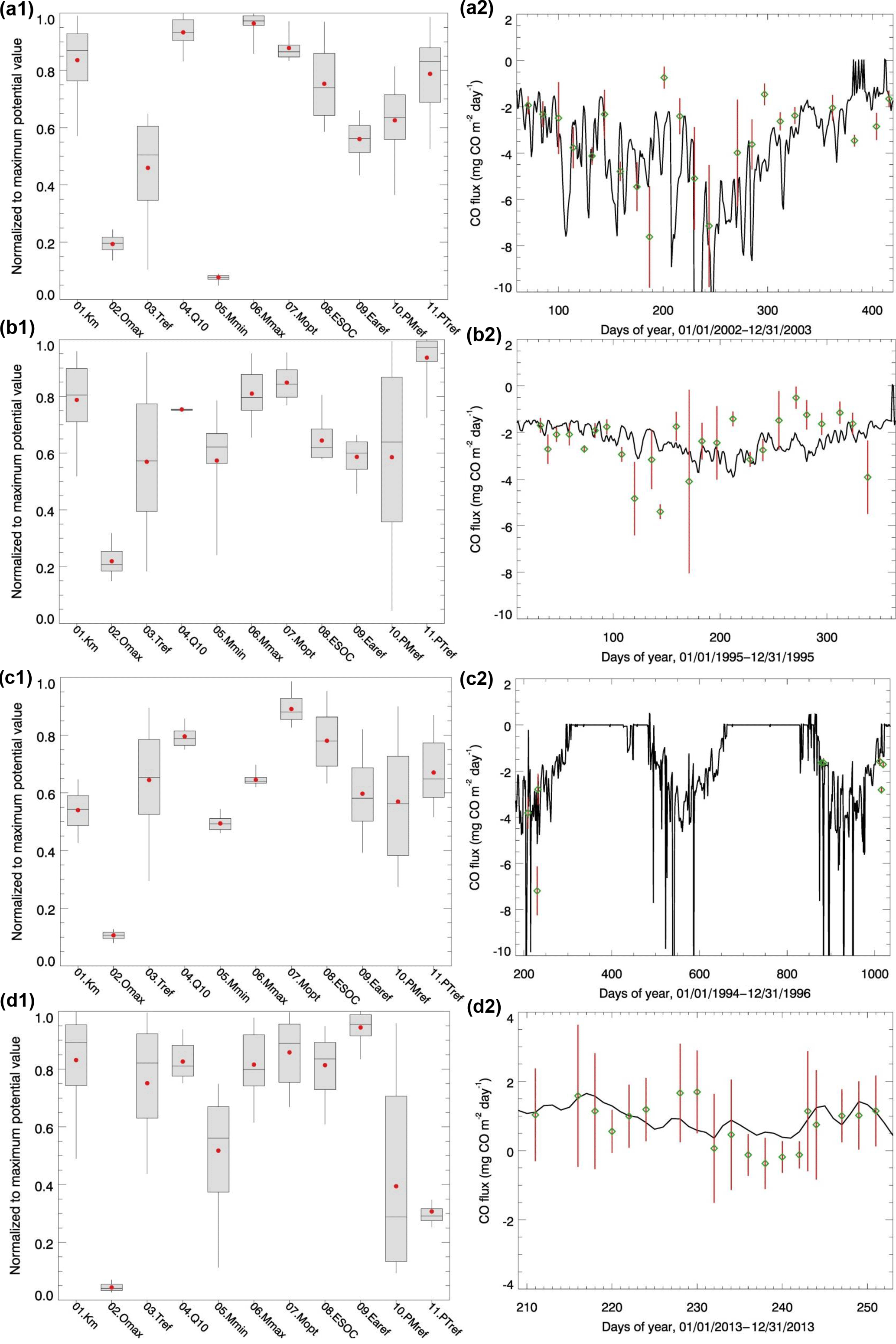
Figure 3Parameter ensemble experiment results: each parameter has 50 calibrated values generated from running SCE-UA-R 50 times independently. Parameters are normalized to their largest potential values described in Table 2. (a1) and (a2) are temperate coniferous forest normalized parameter distribution boxplots and CO flux comparisons between the model simulations (solid line, using the mean value of parameters) and observations (green diamond; red lines represent the error bar, site no. 8), respectively. For each box, line top, box top, horizontal line inside box, box bottom and line bottom represent maximum, third quartile, median, first quartile and minimum of 50 parameter values. Red dot represents the mean value of 50 parameter values. (b1) and (b2) are plots for temperate deciduous forest (site no. 11). Parameter ensemble experiment results: each parameter has 50 calibrated values generated from running SCE-UA-R 50 times independently. Parameters are normalized to their largest potential values described in Table 2. (c1) and (c2) are boreal forest normalized parameter distribution boxplots and CO flux comparisons between the model simulations (solid line, using the mean value of parameters) and observations (green diamond; red lines represent the error bar, site no. 12), respectively. For each box, line top, box top, horizontal line inside box, box bottom and line bottom represent maximum, third quartile, median, first quartile and minimum of 50 parameter values. Red dot represents the mean value of 50 parameter values. (d1) and (d2) are for grassland (site no. 6). Grassland observation data are the sum of hourly observations, so the error bar represents the standard deviation.
2.4 Data organization
To get the spatially and temporally explicit estimates of the CO consumption, production and net flux at the global scale, we used the data of land cover, soils, climate and leaf area index (LAI) from various sources at a spatial resolution of 0.5∘ latitude × 0.5∘ longitude to drive the TEM. The land cover data include the potential vegetation distribution (Melillo et al., 1993) and soil texture (Zhuang et al., 2003), which were used to assign vegetation- and texture-specific parameters to each grid cell.

Figure 4Historical global land surface (excluding the Antarctic area and ocean area) mean climate, and simulated global mean soil moisture, soil temperature and SOC for the period 1901–2013.
For the simulation of the period 1901–2013, the monthly air temperature, precipitation, cloud fraction and vapor pressure data sets from CRU were used to estimate the soil temperature, soil moisture and SOC with the TEM (Fig. 4). The monthly LAI data from the TEM were required to simulate soil moisture (Zhuang et al., 2004). During this time period, we used an empirical function of latitude which was derived from the observed latitudinal distribution of tropospheric carbon monoxide (Badr and Probert, 1994) to calculate the static CO surface concentration distribution (Eq. 7, Potter et al., 1996):
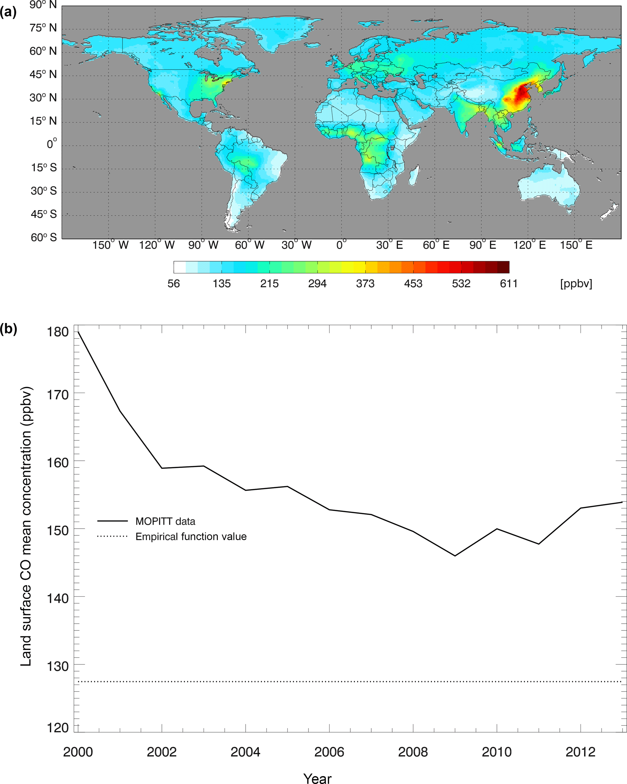
Figure 5CO surface concentration data from the MOPITT satellite (ppbv): (a) the global mean CO surface concentrations from MOPITT during 2000–2013; (b) the CO annual surface concentrations from both MOPITT and empirical functions (Potter et al., 1996).
where CCO,air is the derived surface CO concentration (ppbv), and L represents latitudes with negative degrees for the Southern Hemisphere and positive degrees for the Northern Hemisphere. We also used the atmospheric CO data from the MOPITT satellite during 2000–2013 (Fig. 5). We averaged day-time and night-time monthly mean values of CO surface level 3 retrieval data (variables mapped on 0.5∘ latitude × 0.5∘ longitude grid scales with a monthly time step, Gille, 2013) to represent the CO surface concentration level in each month. The pixels with missing values were filled with the average values of those pixels that were inside 1.5 times of the distance between the missing-value pixel and the nearest pixel with values. These global mean values shown in Fig. 5 do not include ocean surfaces; thus, there are differences between our surface CO concentration results and Yoon and Pozzer's (2014) report in 2014, which is as low as 99.8 ppb. From 2014 to 2100, we used the Intergovernmental Panel on Climate Change (IPCC) future climate scenarios from Representative Concentration Pathways (RCPs) climate forcing data sets RCP2.6, RCP4.5 and RCP8.5 (Fig. 6). RCP2.6, 4.5 and 8.5 data sets are future climate projections with anthropogenic greenhouse gas emission radiative forcings of 2.6, 4.5 and 8.5 W m−2, respectively, by 2100. Since RCPs did not have water vapor pressure data, we used the specific humidity and sea level air pressure from the RCPs and elevation of surface to estimate the monthly surface vapor pressure (Seinfeld and Pandis, 1998).
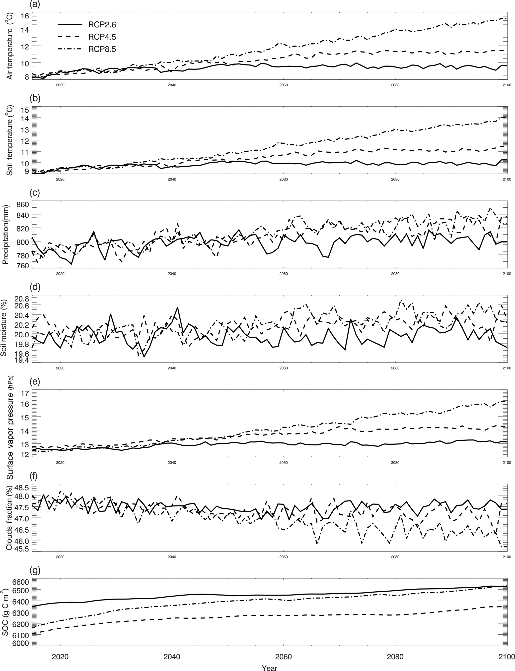
Figure 6Global land surface (excluding the Antarctic area and ocean area) mean climate from the RCP2.6, RCP4.5 and RCP8.5 data sets and simulated mean soil temperature, moisture and SOC: (a–g) are land surface air temperature (∘C), soil temperature (∘C), precipitation (mm), soil moisture (%), surface water vapor pressure (hpa), cloud fraction (%), and SOC (mg m−2), respectively.
2.5 Model experiment design
We conducted two sets of core simulations and eight sensitivity test simulations for a historical period. The two core sets of simulations were driven with the MOPITT CO surface concentration data for the period 2000–2013 (experiment E1) and with the spatially distributed CO surface concentrations assuming them as constant over time estimated from an empirical function of latitude for the period 1901–2100 (experiment E2), respectively. Specifically, in experiment E2 we used the CRU climate forcing for the historical period 1901–2013 and the climate data of RCP2.6, RCP4.5 and RCP8.5 for different future scenarios to examine the responses of CO flux to changing climates. Eight sensitivity simulations were driven with varying different forcing variables while keeping others as they were: (1) with constant CO surface concentrations ± 30 %, (2) SOC ± 5 %, (3) precipitation ± 20 % and (4) air temperature ± 3 ∘C for each pixel, respectively, during 1999–2000 (E3).
3.1 Site evaluation
Both the magnitude and variation of the simulated soil temperature and moisture from cold areas to warm areas compare well to the observations (Fig. 2). The magnitude of the simulated CO flux is comparable and correlated with the observations (R is about 0.5, p-value < 0.001, Fig. 3a2, b2, c2, d2). Estimated CO fluxes for different ecosystem types range from −28.4 to 1.7 mg CO m−2 day−1, and the root mean square error (RMSE) between simulation and observation at all sites is below 1.5 mg CO m−2 day−1. RMSE for site no. 7 is bigger than 2.0 mg CO m−2 day−1 when compared with transparent chamber observations. For the boreal forest site, we only had eight acceptable points in 1994 and 1996 (Fig. 3c2).
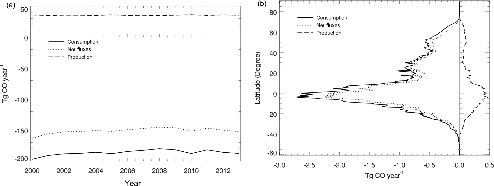
Figure 7Global mean soil CO consumption, production and net flux: (a) the annual time series during 2000–2013 and (b) the latitudinal distribution during 2000–2013.
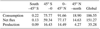
Table 3Regional soil CO consumption, net flux and production (Tg CO yr−1) during 2000–2013.
3.2 Global soil CO dynamics during 2000–2013
Using the MOPITT CO surface concentration data during 2000–2013 (E1), the estimated mean soil CO consumption, production and net flux (positive values indicate CO emissions from soils to the atmosphere) are from −197 to −180, 34 to 36 and −163 to −145 Tg CO yr−1, respectively (Fig. 7a). The consumption is about 4 times larger than the production. The annual consumption and net flux trends follow the atmospheric CO concentration trends (Figs. 5b, 7a), with a small interannual variability (< 10 %). The latitudinal distributions of the consumption, production and net fluxes share the same spatial pattern. Around 20∘ S–20∘ N and 20–60∘ N are the largest and second largest areas for production and consumption, while the 45∘ S–45∘ N area accounts for nearly 90 % of the total consumption and production (Fig. 7b, Table 3). The Southern Hemisphere and Northern Hemisphere have 41 and 59 % of the total consumption, and 47 and 53 % of the total production, respectively (Table 3). The highest rates of the consumption and production are located in areas close to the Equator, and the consumption from areas such as the eastern US, Europe and eastern Asia is also high (< −1000 mg m−2 yr−1) (Fig. 8a, b). Global soils serve as an atmospheric CO sink (Fig. 8c). Some areas, such as the western US and southern Australia, are CO sources, all of which are grasslands or experiencing dry climate. Tropical evergreen forests are the largest sinks, consuming 86 Tg CO yr−1, and tropical savanna and deciduous forest are the second and third largest sinks, consuming a total of 37 Tg CO yr−1 (Table 4). These three ecosystems account for 66 % of the total consumption. Tropical evergreen forests are also the largest source of soil CO production, producing 16 Tg CO yr−1, while tropical savanna has a considerable production of 6 Tg CO yr−1 (Table 4). Moreover, tropical areas, including forested wetlands, forested floodplain and evergreen forests, are most efficient for the CO consumption, ranging from −18 to −13 mg CO m−2 day−1. They are also most efficient for the CO production, at over 2 mg CO m−2 day−1 (Table 4, calculated by fluxes divided by area).
Table 4Annual total soil CO consumption, net flux and production in different ecosystems during 2000–2013 (E1) and mean CO deposition velocity in different ecosystems during 1901–2013 (E2).
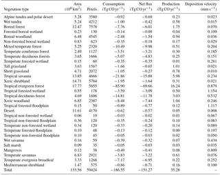

Figure 8Global annual mean soil CO fluxes (mg CO m−2 yr−1) during 2000–2013 using the MOPITT CO atmospheric surface concentration data.
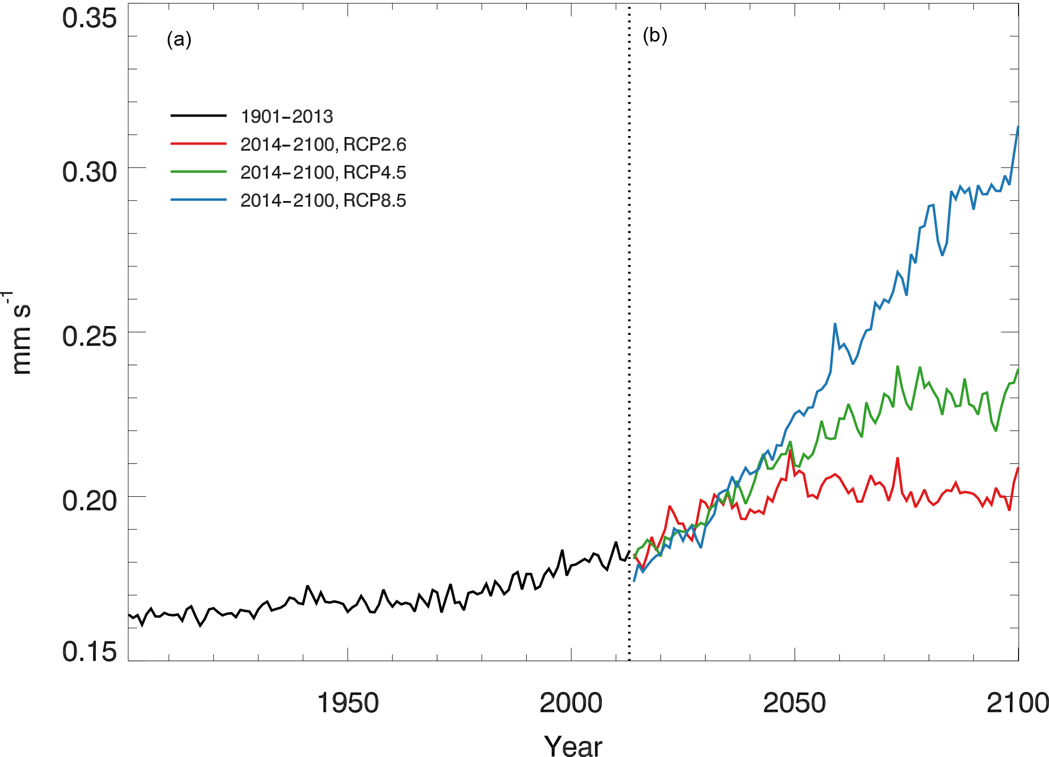
Figure 9Global mean annual time series of CO deposition velocity (mm s−1) using constant in time and spatially distributed CO concentration data during 1901–2013 (a) and under the future climate scenarios RCP2.6, RCP4.5 and RCP8.5 during 2014–2100 (b).
3.3 Global soil CO dynamics during 1901–2100
Using the constant CO surface concentration, the estimated global mean CO deposition velocities are 0.16–0.19 mm s−1 for the period 1901–2013. For the period 2014–2100, the deposition velocities are 0.18–0.21, 0.18–0.24 and 0.17–0.31 for the RCP2.6, 4.5 and 8.5 scenarios, respectively (Fig. 9). During 2014–2100, there are significant trends of increasing deposition velocities for nearly all scenarios (Fig. 9). The rates of increase are 0.0002, 0.0005 and 0.0013 mm s−1 yr−1, and will reach 0.20, 0.23 and 0.30 mm s−1 by the end of the 21st century for the RCP2.6, RCP4.5 and RCP8.5 scenarios, respectively (Fig. 9). These increasing trends are similar to the air temperature increasing trends (Fig. 6a). The global distribution patterns of the CO deposition velocity are similar to the net flux distribution for the period 2000–2013, but there are significant differences between the 1901–2013, RCP2.6, RCP4.5 and RCP8.5 scenarios (Fig. 10). The deposition velocities increase from the RCP2.6 to RCP8.5 and larger than that in the historical periods in areas near the Equator (Fig. 10). Areas near the Equator and eastern Asia become big sinks of the atmospheric CO, while the northeastern US becomes a small source in the 21st century (Fig. 10). Different vegetation types have a large range of the deposition velocity, from 0.008 to 1.154 mm s−1 (Table 4). The tropical forested wetland, tropical forested floodplain and tropical evergreen forest have the top three largest deposition velocities of 1.154, 1.117 and 0.879 mm s−1, respectively, while desert, short grasslands, and wet tundra have the smallest deposition velocities of 0.008, 0.010 and 0.015 mm s−1, respectively.
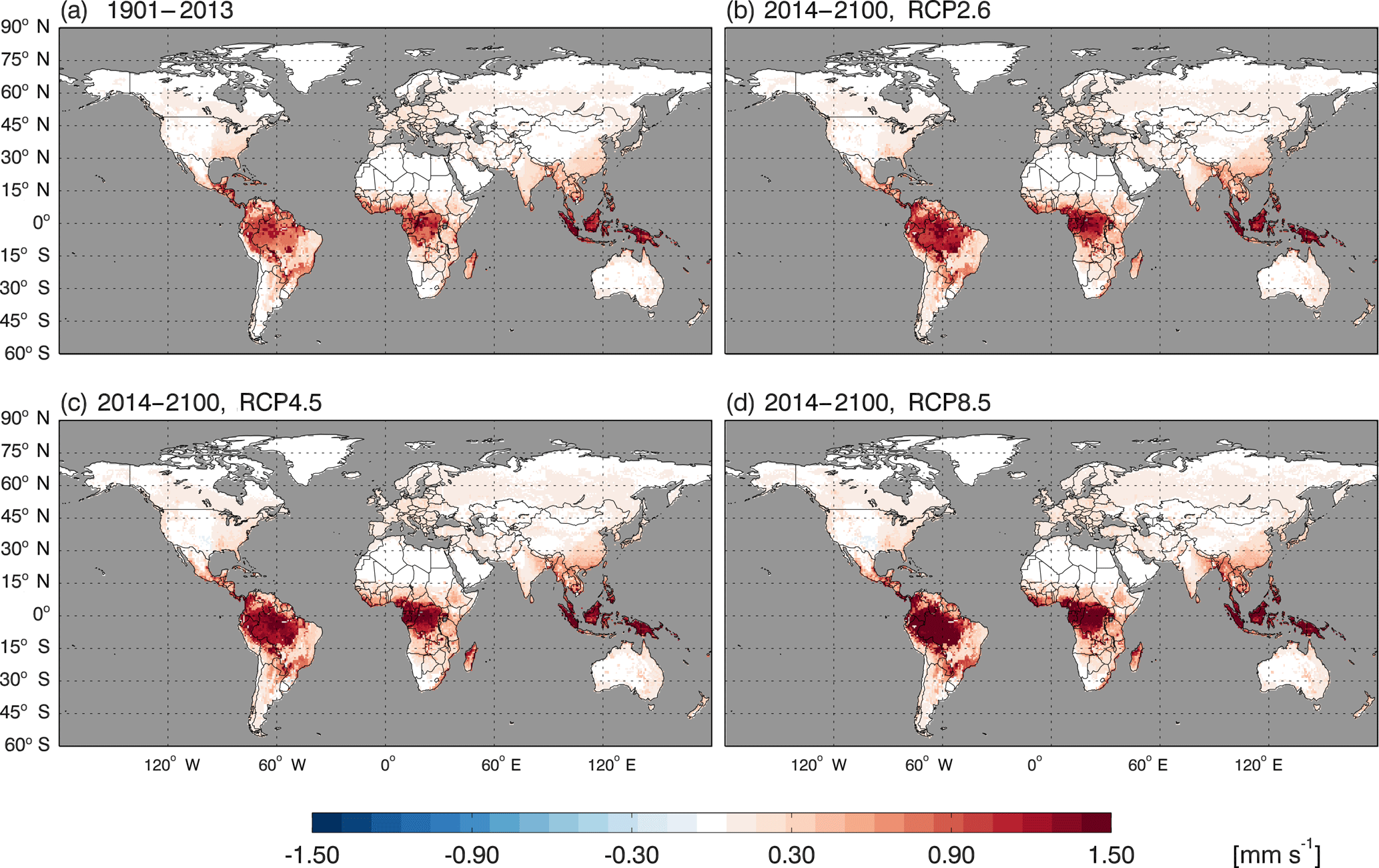
Figure 10Global annual mean CO deposition velocity using constant in time and spatially distributed CO concentration data (mm s−1) (a) during 1901–2013 and (b), (c), (d) under the future climate scenarios RCP2.6, RCP4.5 and RCP8.5 during 2014–2100, respectively.
3.4 Sensitivity test
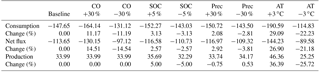
The soil CO consumption is most sensitive (changing 29 %) to air temperature, while the production is most sensitive to both air temperature (changing up to 36 %) and SOC (5 %). The net CO fluxes have similar sensitivities to the consumption. The annual CO consumption, production and net flux follow the change in air temperature (Table 5). In addition, a 30 % change in precipitation will not lead to large changes in the CO flux (< 3 %).
Table 5Sensitivity of the global CO consumption, net flux and production (Tg CO yr−1) to the changes in atmospheric CO, soil organic carbon (SOC), precipitation (Prec) and air temperature (AT).
4.1 Comparison with other studies
Previous studies estimated a wide range of the global CO consumption from −16 to −640 Tg CO yr−1. Our estimates are from −197 to −180 Tg CO yr−1 for 2000–2013 using the MOPITT satellite CO surface concentration data. Previous studies also provided a large range for the CO production from 0 to 7.6 mg m−2 day−1 (reviewed in Pihlatie et al., 2016). Our results showed the averaged CO production ranging from 0.01 to 2.29 mg m−2 day−1. The existing estimates of the CO deposition velocities for different vegetation types ranged from 0.0 to 4.0 mm s−1, while our simulations showed an averaged CO deposition velocity ranging from 0.006 to 1.154 mm s−1 for different vegetation types. The large uncertainty of these estimates is mainly due to different considerations of the microbial activities, the depth of the soil, and the parameters in the model. In contrast to the estimates of −57 to −16 Tg CO yr−1 which were based on the top 5 cm of soils (Potter et al., 1996), our estimates considered 30 cm soils, which were used in Whalen and Reeburgh (2001). In addition, we used a thinner layer division (1 cm for each layer) for the diffusion process, and used the Crank–Nicolson method to solve partial differential equations to avoid time step influences. We also included the microbial CO oxidation process to remove the CO from the soil and considered the effects of soil moisture, soil temperature, vegetation type and soil CO substrate on microbial activities. Our soil thermal, soil hydrology and carbon and nitrogen dynamics simulated in the TEM provided carbon substrate spatially and temporally for estimating the soil CO dynamics. Overall, although a few previous studies have examined the long-term impacts of climate, land use and nitrogen deposition on the CO dynamics (Chan and Steudler, 2006, Pihlatie et al., 2016), the global prediction of the soil CO dynamics still has a large uncertainty.
4.2 Major controls on soil CO dynamics
The sensitivity tests indicate that the consumption is normally much larger than the CO production, so that the former will determine the dynamics of the net flux (Table 5). The model being sensitive to air temperature explains the small increasing trends after the 1960s, the significant increasing trend in the 21st century and the large sinks over tropical areas (Table 5, Fig. 9). SOC did not directly influence the CO consumption. For instance, increasing SOC led to an increase in the soil CO substrate, implying that more CO in soils can be consumed. An extra 3 Tg CO yr−1 was taken up from the atmosphere to the soil in the sensitivity test when SOC increased by 5 % (Table 5), which will be discussed in detail in Sect. 4.3. CO surface concentrations will only influence the uptake rate and soil CO substrate concentrations, thus influencing the soil CO consumption rate.
Table 6Correlation coefficients between forcing variables (precipitation (Prec), air temperature (Tair), soil organic carbon (SOC), soil temperature (Tsoil), soil moisture (Msoil) and atmospheric CO (CO air)) and absolute values of consumption, production and net flux for different regions and the globe.
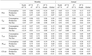
The annual CO consumption and net flux have a similar correlation coefficient with forcing variables and both are significantly correlated with air temperature, soil temperature SOC and atmospheric CO concentration (R>0.91 globally, Table 6). Increasing temperature will increase microbial activities, while more SOC will increase soil CO substrate level. The annual CO consumption and net flux have low correlations with annual precipitation and soil moisture, especially at 45∘ N–45∘ S (R<0.54, Table 6). The annual CO production is strongly correlated with annual mean SOC, air temperature and soil temperature (R<0.91), while it is less correlated with precipitation, soil moisture and atmospheric CO concentration. Meanwhile, the monthly CO consumption, production and net flux are well correlated with air temperature, soil temperature, precipitation, and soil moisture (R>0.69 globally, Table 6). The soil moisture is significantly influenced by temperature at a monthly time step since the increasing temperature would induce higher evapotranspiration. The monthly CO consumption, production and net flux have low correlations with SOC because it will not change greatly within a month.

Figure 11Global mean monthly time series of the MOPITT surface atmospheric CO concentration (ppbv) and soil CO consumption from model simulations E1 (Tg CO mon−1).
The R between the annual soil CO consumption and atmospheric CO concentration is 0.91 at the global scale because the atmospheric CO concentration, air temperature, and soil temperature dominate the annual consumption rate. At a monthly scale, this R is −0.48 because the global atmospheric CO concentrations are high in winter and low in summer, while the simulated soil CO consumption shows an opposite monthly variation (Table 6, Fig. 11), suggesting that other factors such as precipitation, air temperature, and soil temperature are major controls for the monthly CO fluxes.
4.3 Model uncertainties and limitations
There are a number of limitations, contributing to our simulation uncertainties. First, due to lacking long-period observational data of the CO flux and associated environmental factors, the model parameterization can only be conducted for four ecosystem types, including boreal forest, temperate coniferous forest, temperate deciduous forest, and grassland. Tropical forest calibration is only conducted using a very limited amount of laboratory experiment data, but tropical areas are hotspots for CO soil–atmosphere exchanges. Besides, the amount of tropical forest SOC for the top 30 cm can be very large according to observations. The TEM may underestimate the top 30 cm SOC, which will underestimate the production rates, especially in tropical regions. Tropical regions typically have high temperature during the whole year, which may result in overestimation of the CO consumption using Eq. (2b). The large deviation of model simulations to observations in tropical savanna (which is a mosaic of tropical forest and grassland ecosystems) may be due to using outside air temperature to represent inside air temperature of transparent chamber observations (Varella et al., 2004), and uncertain tropical forest parameterization. Second, we used the conclusion from van Asperen et al. (2015) and only considered the thermal-degradation process for the CO production in this study. The photo-degradation process and biological formation process were not considered due to a lack of understanding of these processes. Third, the static CO surface concentration derived from the empirical function is lower than the MOPITT CO surface concentration, which will lead to underestimation of CO deposition velocity during 1901–2100. Fourth, from the sensitivity test (Table 5) we notice that an increase in SOC by 5 % resulted in a net flux increase from the atmosphere to the soil by 2.57 %. The SOC increase enhanced CO production (Eq. 3), CO concentrations (Eq. 1), and CO oxidation (Eq. 2). When the change in total oxidation is larger than the difference between the change in total production and the change in total soil CO concentration (Eq. 1), the estimate of the net flux change is negative (from the atmosphere to soil) using a mass balance approach (Sect. 2.2), which leads to a 2.57 % increase in the net flux in our SOC sensitive test. This is due to the fact that CO production (Eq. 3) is calculated independently from oxidation (Eq. 2). This will not influence our general findings since SOC varies only slightly during our simulation periods, with a 3 % increase from 1900 to 2013 (Fig. 4d) and up to a 4 % increase from 2014 to 2100 (Fig. 6g). This model artifact that is apparent in the SOC sensitivity test can be alleviated using a very fine time step (e.g., 1 s), because in this case CO concentrations change only slightly within the short time. Therefore, when a short time step is used, the net flux roughly equals the difference between production and oxidation. If the change in production is bigger than the change in oxidation, the change in net flux will be positive, leading to a decrease in deposition to the soil. The downside is that running the model at a time step of 1 s will require a significantly large amount of computing time. Fifth, our model structure still has a large potential to improve. In this study we divided the top 30 cm soil into 30 layers (layer thickness dz = 1 cm), but a finer division will increase the accuracy (Fig. 12). We chose 1 cm thickness because if thicker than 1 cm, the model vertical CO concentration profile will deviate from reality and the diffusion process will be influenced significantly. If thinner than 1 cm, it will need much more computing time but will not have much improvement compared to the thickness set to 1 cm (Fig. 12a–e). We notice that the 30-layer division represents the soil CO concentration profile well, not only in the days of soil CO net uptake, but also in the days of CO net emission (Fig. 12c, f). Sixth, the Michaelis–Menten function (Eq. 2a) is used in this model and we notice that kCO is normally much larger than C(t,i) in those days of net soil uptake (over 10 times larger, Fig. 12). However, we cannot simplify Eq. (2b) to , because the CO concentrations in the soil can be larger than in the atmosphere in the days of net emissions and C(t,i) may be close to kCO, and then the simplified equation may lead to overestimation of CO oxidation (Fig. 12f). Finally, although we focused on natural ecosystems in this study, the land-use change, agriculture activity, and nitrogen deposition also affect the soil CO consumption and production (King and Crosby, 2002; Chan and Steudler, 2006). For instance, the soil CO consumption in agriculture ecosystems is from 0 to 9 mg CO m−2 day−1 in Brazil (King and Hungria, 2002). In this study, we used grassland or forest ecosystems to represent agriculture areas in the CODM module. Our future study will include these processes and factors.
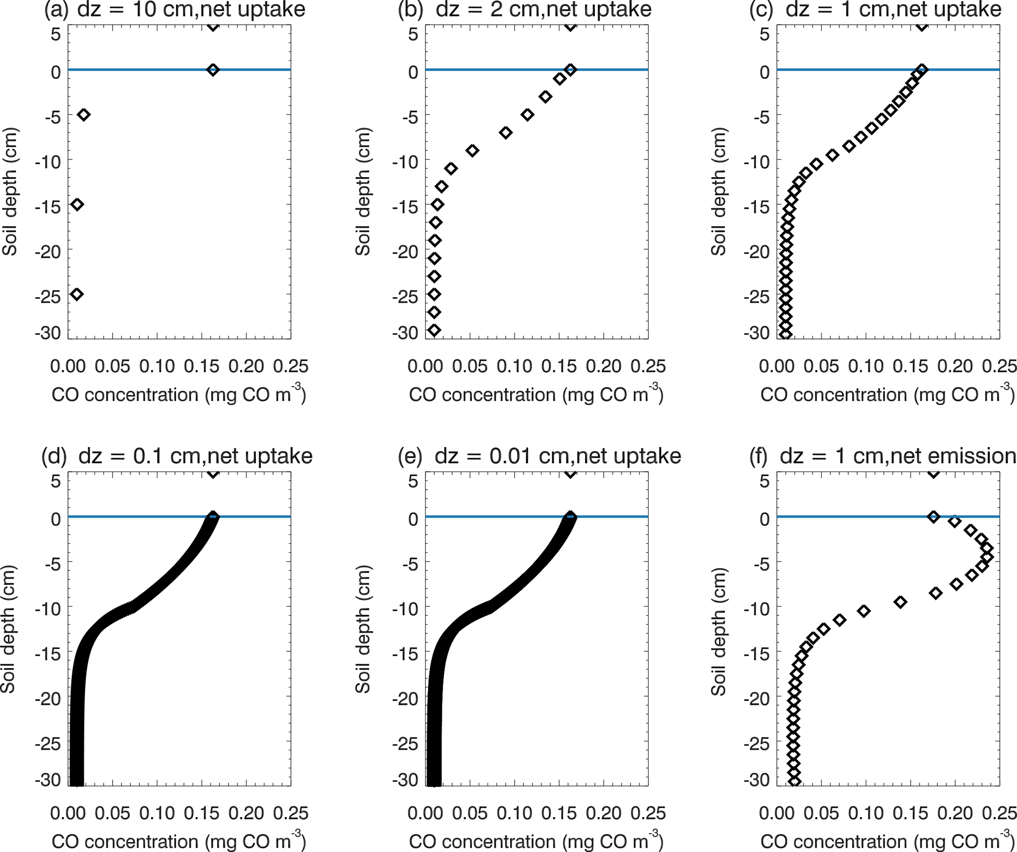
Figure 12Daily mean vertical soil CO concentration profiles of the top 30 cm. In the soil (depth < 0 cm), black diamonds represent the soil CO concentration (mg CO m−3). Above the surface (depth > = 0 cm), black diamonds represent the atmospheric CO concentration. (a), (b), (c), (d) and (e) are the results from the same day when soils are a net sink of CO, but using different layer thicknesses (dz = 10, 2, 1, 0.1 and 0.01 cm, respectively); (f) is the result from the day when soils are a net source of CO, with dz = 1 cm.
We analyzed the magnitude, spatial pattern, and controlling factors of the atmosphere–soil CO exchanges at the global scale for the 20th and 21st centuries using a process-based biogeochemistry model. Major processes include the atmospheric CO diffusion from the atmosphere to the soil and inside the soil of terrestrial ecosystems, microbial oxidation removal of CO, and CO production through chemical reaction. We found that air temperature and soil temperature play a dominant role in determining the annual soil CO consumption and production, while precipitation, air temperature, and soil temperature are the major controls for the monthly consumption and production. The atmospheric CO concentrations are important for annual CO consumption. We estimated that the global annual CO consumption, production and net fluxes for 2000–2013 are from −197 to −180, 34 to 36 and −163 to −145 Tg CO yr−1, respectively, when using the MOPITT CO surface concentration data. Tropical evergreen forest, savanna and deciduous forest areas are the largest sinks, accounting for 66 % of the total CO consumption, while the Northern Hemisphere consumes 59 % of the global total. During the 20th century, the estimated CO deposition velocity is 0.16–0.19 mm s−1. The predicted CO deposition velocity will reach 0.20–0.30 mm s−1 in the 2090s, primarily because of the increasing air temperature. The areas near the Equator, eastern Asia, Europe and the eastern US will become the hotspots of sinks because they have warm and moist soils. This study calls for long-period observations of CO flux for various ecosystem types and better projection of atmospheric CO surface concentrations from 1901 to 2100 to improve future estimates of global soil CO consumption. The effects of land-use change, agriculture activities, nitrogen deposition, photo-degradation and biological formation will also be considered to improve future quantification of soil CO fluxes.
All data used in this study are available from the authors upon request.
The authors declare that they have no conflict of interest.
This study is supported through projects funded to Qianlai
Zhuang by the Department of Energy
(DE-SC0008092 and DE-SC0007007) and the NSF Division of Information and
Intelligent Systems (NSF-1028291). The supercomputing resource is provided by
the Rosen Center for Advanced Computing at Purdue University. We acknowledge
Stephen C. Whalen for making the observational CO flux data available to this
study. We are also grateful to the University of Tuscia (dep. DIBAF), Italy,
and their affiliated members, for their help and the use of their field
data.
Edited by: Thomas
Röckmann
Reviewed by: Seiichiro Yonemura and one anonymous
referee
Amiro, B.: AmeriFlux CA-Man Manitoba – Northern Old Black Spruce (former BOREAS Northern Study Area) [Data set], AmeriFlux, University of Manitoba, https://doi.org/10.17190/amf/1245997, 2016.
Badr, O. and Probert, S. D.: Carbon monoxide concentration in the Earth's atmosphere, Appl. Energ., 49, 99–143, https://doi.org/10.1016/0306-2619(94)90035-3, 1994.
Bergamaschi, P., Hein, R., Heimann, M., and Crutzen, P. J.: Inverse modeling of the global CO cycle: 1. Inversion of CO mixing ratios, J. Geophys. Res.-Atmos., 105, 1909–1927, https://doi.org/10.1029/1999jd900818, 2000.
Bonan, G.: A Land Surface Model (LSM Version 1.0) for Ecological, Hydrological, and Atmospheric Studies: Technical Description and User's Guide, UCAR/NCAR, NCAR/TN-417+STR, https://doi.org/10.5065/d6df6p5x, 1996.
Bourgeau-Chavez, L. L., Garwood, G. C., Riordan, K., Koziol, B. W., and Slawski, J.: Development of calibration algorithms for selected water content reflectometry probes for burned and nonburned organic soils of Alaska, Int. J. Wildland Fire, 19, 961e975, https://doi.org/10.1071/wf07175, 2012.
Bruhn, D., Albert, K. R., Mikkelsen, T. N., and Ambus, P.: UV-induced carbon monoxide emission from living vegetation, Biogeosciences, 10, 7877–7882, https://doi.org/10.5194/bg-10-7877-2013, 2013.
Castellanos, P., Marufu, L. T., Doddridge, B. G., Taubman, B. F., Schwab, J. J., Hains, J. C., and Dickerson, R. R.: Ozone, oxides of nitrogen, and carbon monoxide during pollution events over the eastern United States: An evaluation of emissions and vertical mixing, J. Geophys. Res.-Atmos., 116, D16307, https://doi.org/10.1029/2010JD014540, 2011.
Chan, A. S. K. and Steudler, P. A.: Carbon monoxide uptake kinetics in unamended and long-term nitrogen-amended temperate forest soils, FEMS Microbiol. Ecol., 57, 343–354, https://doi.org/10.1111/j.1574-6941.2006.00127.x, 2006.
Conrad, R.: Biogeochemistry and ecophysiology of atmospheric CO and H2, Adv. Microb. Ecol., 10, 231–283, https://doi.org/10.1007/978-1-4684-5409-3_7, 1988.
Conrad, R. and Seiler, W.: Characteristics of abiological carbon monoxide formation from soil organic matter, humic acids, and phenolic compounds, Environ. Sci. Technol., Am. Chem. Soc. (ACS), 19, 1165–1169, https://doi.org/10.1021/es00142a004, 1985.
Crutzen, P. J. and Giedel, L. T.: A two-dimensional photochemical model of the atmosphere. 2: The tropospheric budgets of anthropogenic chlorocarbons CO, CH4, CH3Cl and the effect of various NOx sources on tropospheric ozone, J. Geophys. Res., 88, 6641–6661, https://doi.org/10.1029/JC088iC11p06641, 1983.
Crutzen, P. J.: Role of the tropics in atmospheric chemistry, The Geophysiology of Amazonia Vegetation Climate Interaction (Dickinson RE, ed.), 107–131, John Wiley, New York, 1987.
Dee, D. P., Uppala, S. M., Simmons, A. J., Berrisford, P., Poli, P., Kobayashi, S., and Vitart, F.: The ERA-Interim reanalysis: configuration and performance of the data assimilation system, Q. J. Roy. Meteorol. Soc., 137, 553–597, https://doi.org/10.1002/qj.828, 2011.
Derendorp, L., Quist, J. B., Holzinger, R., and Röckmann, T.: Emissions of H2 and CO from leaf litter of Sequoiadendron giganteum, and their dependence on UV radiation and temperature, Atmos. Environ., 45, 7520–7524, https://doi.org/10.1016/j.atmosenv.2011.09.044, 2011.
Duan, Q. Y., Gupta, V. K., and Sorooshian, S.: Shuffled complex evolution approach for effective and efficient global minimization, J. Optim. Theor. Appl., 76, 501–521, https://doi.org/10.1007/BF00939380, 1993.
Emmons, L. K., Walters, S., Hess, P. G., Lamarque, J.-F., Pfister, G. G., Fillmore, D., Granier, C., Guenther, A., Kinnison, D., Laepple, T., Orlando, J., Tie, X., Tyndall, G., Wiedinmyer, C., Baughcum, S. L., and Kloster, S.: Description and evaluation of the Model for Ozone and Related chemical Tracers, version 4 (MOZART-4), Geosci. Model Dev., 3, 43–67, https://doi.org/10.5194/gmd-3-43-2010, 2010.
Fisher, M. E.: Soil-atmosphere Exchange of Carbon Monoxide in Forest Stands Exposed to Elevated and Ambient CO2, Undergraduate Honors Thesis, University of North Carolina, Chapel Hill NC, available at: https://search.lib.unc.edu:443/search?R=UNCb4424718 (last access: 4 June 2018), 2003.
Fraser, W. T., Blei, E., Fry, S. C., Newman, M. F., Reay, D. S., Smith, K. A., and McLeod, A. R.: Emission of methane, carbon monoxide, carbon dioxide and short-chain hydrocarbons from vegetation foliage under ultraviolet irradiation, Plant, Cell Environ., 38, 980–989, https://doi.org/10.1111/pce.12489, 2015.
Funk, D. W., Pullman, E. R., Peterson, K. M., Crill, P. M., and Billings, W. D.: Influence of water table on carbon dioxide, carbon monoxide, and methane fluxes from Taiga Bog microcosms, Global Biogeochem. Cy., 8, 271–278, https://doi.org/10.1029/94GB01229, 1994.
Gille, J.: MOPITT Gridded Monthly CO Retrievals (Near and Thermal Infrared Radiances) – Version 6 [Data set], NASA Langley Atmospheric Science Data Center, https://doi.org/10.5067/TERRA/MOPITT/DATA301, 2013.
Harris, I., Jones, P. D., Osborn, T. J., and Lister, D. H.: Updated high-resolution grids of monthly climatic observations – the CRU TS3.10 Dataset, Int. J. Climatol., 34, 623–642, https://doi.org/10.1002/joc.3711, 2013.
He, H. and He, L.: The role of carbon monoxide signaling in the responses of plants to abiotic stresses, Nitric Oxide?: Biology and Chemistry/Official Journal of the Nitric Oxide Society, 42, 40–43, https://doi.org/10.1016/j.niox.2014.08.011, 2014.
Jobbagy, E. G. and Jackson, R.: The vertical Distribution of soil organic carbon and its relation to climate and vegetation, Ecol. Appl., 10:2(April), 423–436, https://doi.org/10.2307/2641104, 2000.
Khalil, M. A. K. and Rasmussen, R. A.: The global cycle of carbon monoxide: Trends and mass balance, Chemosphere, 20, 227–242, https://doi.org/10.1016/0045-6535(90)90098-E, 1990.
Khalil, M. A., Pinto, J., and Shearer, M.: Atmospheric carbon monoxide, Chemosphere - Global Change Science, Elsevier BV, doi:s1465-9972(99)00053-7, 1999.
King, G. M.: Characteristics and significance of atmospheric carbon monoxide consumption by soils, Chemosphere, 1, 53–63, https://doi.org/10.1016/S1465-9972(99)00021-5, 1999a.
King, G. M.: Attributes of Atmospheric Carbon Monoxide Oxidation by Maine Forest Soils, Appl. Environ. Microbiol., 65, 5257–5264, 1999b.
King, G. M.: Land use impacts on atmospheric carbon monoxide consumption by soils, Global Biogeochem. Cy., 14, 1161–1172, https://doi.org/10.1029/2000GB001272, 2000.
King, G. M. and Crosby, H.: Impacts of plant roots on soil CO cycling and soil-atmosphere CO exchange, Global Change Biol., 8, 1085–1093, https://doi.org/10.1046/j.1365-2486.2002.00545.x, 2002.
King, G. M. and Hungria, M.: Soil-atmosphere CO exchanges and microbial biogeochemistry of CO transformations in a Brazilian agricultural ecosystem, Appl. Environ. Microbiol., 68, 4480–4485, https://doi.org/10.1128/AEM.68.9.4480-4485.2002, 2002.
King, G. M. and Weber, C. F.: Distribution, diversity and ecology of aerobic CO-oxidizing bacteria, Nature Reviews, Microbiology, 5, 107–18, https://doi.org/10.1038/nrmicro1595, 2007.
King, J. Y., Brandt, L. A., and Adair, E. C.: Shedding light on plant litter decomposition: advances, implications and new directions in understanding the role of photodegradation, Biogeochem., 111, 57–81, https://doi.org/10.1007/s10533-012-9737-9, 2012.
Kuhlbusch, T. A., Zepp, R. G., Miller, W. L., and Burke, R. A. Jr.: Carbon monoxide fluxes of different soil layers in upland Canadian boreal forests, Tellus B, Informa UK Limited, 50, 353–365, https://doi.org/10.1034/j.1600-0889.1998.t01-3-00003.x, 1998
Lamarque, J.-F., Emmons, L. K., Hess, P. G., Kinnison, D. E., Tilmes, S., Vitt, F., Heald, C. L., Holland, E. A., Lauritzen, P. H., Neu, J., Orlando, J. J., Rasch, P. J., and Tyndall, G. K.: CAM-chem: description and evaluation of interactive atmospheric chemistry in the Community Earth System Model, Geosci. Model Dev., 5, 369–411, https://doi.org/10.5194/gmd-5-369-2012, 2012.
Lee, H., Rahn, T., and Throop, H.: An accounting of C-based trace gas release during abiotic plant litter degradation, Global Change Biol., 18, 1185–1195, https://doi.org/10.1111/j.1365-2486.2011.02579.x, 2012.
Logan, J. A., Prather, M. J., Wofsy, S. C., and McElroy, M. B.: Tropospheric chemistry – A global perspective, J. Geophys. Res., 86, 7210–7254, https://doi.org/10.1029/JC086iC08p07210, 1981.
Lu, Y. and Khalil, M. A. K.: Methane and carbon monoxide in OH chemistry: The effects of feedbacks and reservoirs generated by the reactive products, Chemosphere. Elsevier BV, 26, 641–655, https://doi.org/10.1016/0045-6535(93)90450-j, 1993.
Melillo, J. M., McGuire, A. D., Kicklighter, D. W., Moore, B., Vorosmarty, C. J., and Schloss, A. L.: Global climate change and terrestrial net primary production, Nature, 363, 234, 1993.
Moxley, J. M. and Smith, K. A.: Factors affecting utilisation of atmospheric CO by soils, Soil Biol. Biochem., 30, 65–79, https://doi.org/10.1016/S0038-0717(97)00095-3, 1998.
Myhre, G., Shindell, D., Bréon, F. M., Collins, W., Fuglestvedt, J., Huang, J., and Nakajima, T.: Anthropogenic and Natural Radiative Forcing. In: Climate Change 2013: The Physical Science Basis, Contribution of Working Group 1 to the Fifth Assessment Report of the Intergovernmental Panel on Climate Change, Table, 8, 714, 2013.
Nakai, T., Kim, Y., Busey, R. C., Suzuki, R., Nagai, S., Kobayashi, H., and Ito, A.: Characteristics of evapotranspiration from a permafrost black spruce forest in interior Alaska, Polar Sci., 7, 136–148, https://doi.org/10.1016/j.polar.2013.03.003, 2013.
Novick, K., Oishi, C., and Stoy, P.: AmeriFlux US-Dk3 Duke Forest – loblolly pine [Data set], AmeriFlux; Indiana University; Montana State University, USDA Forest Service, https://doi.org/10.17190/amf/1246048, 2016.
Philip, R. and Novick, K.: AmeriFlux US-MMS Morgan Monroe State Forest [Data set], AmeriFlux; Indiana University, https://doi.org/10.17190/AMF/1246080, 2016.
Pihlatie, M., Rannik, Ü., Haapanala, S., Peltola, O., Shurpali, N., Martikainen, P. J., Lind, S., Hyvönen, N., Virkajärvi, P., Zahniser, M., and Mammarella, I.: Seasonal and diurnal variation in CO fluxes from an agricultural bioenergy crop, Biogeosciences, 13, 5471–5485, https://doi.org/10.5194/bg-13-5471-2016, 2016.
Potter, C. S., Klooster, S. A., and Chatfield, R. B.: Consumption and production of carbon monoxide in soils: A global model analysis of spatial and seasonal variation, Chemosphere, 33, 1175–1193, https://doi.org/10.1016/0045-6535(96)00254-8, 1996.
Prather, M. and Ehhalt, D.: Atmospheric chemistry and greenhouse gases. Climate Change, 2001: The Scientific Basis, edited by: Houghton, J. T., Ding, Y., Griggs, D. J., Noguer, M., van der Linden, P. J., Dai, X., Maskell, K., and Johnson, C. A., 239–288, Cambridge University Press, Cambridge, UK, 2001.
Prather, M., Derwent, R., Ehhalt, D., Fraser, P., Sanheeza, E., and Zhou, X.: Other trace gases and atmospheric chemistry, Climate Change, 1994, Radiative Forcing of Climate Change, edited by: Houghton, J. T., Meira Filho, L. G., Bruce, J., Hoesung Lee, B. A., Callander, E., Haites, E., Harris, N., and Maskell, K., 76–126, Cambridge University Press, Cambridge, UK, 1995.
Saleska, S. R., Da Rocha, H. R., Huete, A. R., Nobre, A. D., Artaxo, P. E., and Shimabukuro, Y. E.: LBA-ECO CD-32 Flux Tower Network Data Compilation, Brazilian Amazon: 1999–2006, ORNL Distributed Active Archive Center, https://doi.org/10.3334/ORNLDAAC/1174, 2013.
Sanderson, M. G., Collins, W. J., Derwent, R. G., and Johnson, C. E.: Simulation of global hydrogen levels using a Lagrangian three-dimensional model, J. Atmos. Chem., 46, 15–28, https://doi.org/10.1023/A:1024824223232, 2003.
Sanhueza, E., Dong, Y., Scharffe, D., Lobert, J. M., and Crutzen, P. J.: Carbon monoxide uptake by temperate forest soils: The effects of leaves and humus layers, Tellus, B, 50, 51–58, https://doi.org/10.1034/j.1600-0889.1998.00004.x, 1998.
Schade, G. W. and Crutzen, P. J.: CO emissions from degrading plant matter (II). Estimate of a global source strength, Tellus B, 51, 909–918, https://doi.org/10.1034/j.1600-0889.1999.t01-4-00004.x, 1999.
Scharffe, D., Hao, W. M., Donoso, L., Crutzen, P. J., and Sanhueza, E.: Soil fluxes and atmospheric concentration of CO and CH4 in the northern part of the Guayana shield, Venezuela, J. Geophys. Res.-Atmos., 95, 22475–22480, https://doi.org/10.1029/JD095iD13p22475, 1990.
Seiler, W.: in: Environmental Biogeochemistry and Geomicrobiology, Methods, Metals and Assessment, edited by: Krumbein, W. E., Vol. 3, Ann Arbor Science, Ann Arbor, MI, 773–810, 1987.
Seinfeld, J. H. and Pandis, S. N.: Atmospheric Chemistry and Physics: From Air Pollution to Climate Change, Atmospheric Chemistry and Physics from Air Pollution to Climate Change Publisher New York NY Wiley 1998 Physical Description Xxvii 1326, A WileyInterscience Publication, ISBN0471178152, 51, 1–4, https://doi.org/10.1080/00139157.1999.10544295, 1998.
Stein, O., Schultz, M. G., Bouarar, I., Clark, H., Huijnen, V., Gaudel, A., George, M., and Clerbaux, C.: On the wintertime low bias of Northern Hemisphere carbon monoxide found in global model simulations, Atmos. Chem. Phys., 14, 9295–9316, https://doi.org/10.5194/acp-14-9295-2014, 2014.
Stevenson, D. S., Dentener, F. J., Schultz, M. G., Ellingsen, K., van Noije, T. P. C., Wild, O., and Szopa, S.: Multimodel ensemble simulations of present-day and near-future tropospheric ozone, J. Geophys. Res.-Atmos., 111, D08301, https://doi.org/10.1029/2005JD006338, 2006.
Suzuki, R.: AmeriFlux US-Prr Poker Flat Research Range Black Spruce Forest [Data set], AmeriFlux; Japan Agency for Marine-Earth Science and Technology, https://doi.org/10.17190/AMF/1246153, 2016.
Tan, Z. and Zhuang, Q.: An analysis of atmospheric CH4 concentrations from 1984 to 2008 with a single box atmospheric chemistry model, Atmos. Chem. Phys. Discuss., 12, 30259–30282, https://doi.org/10.5194/acpd-12-30259-2012, 2012.
Tarr, M. A., Miller, W. L., and Zepp, R. G.: Direct carbon monoxide photoproduction from plant matter, J. Geophys. Res., 100, 11403, https://doi.org/10.1029/94JD03324, 1995.
van Asperen, H., Warneke, T., Sabbatini, S., Nicolini, G., Papale, D., and Notholt, J.: The role of photo- and thermal degradation for CO2 and CO fluxes in an arid ecosystem, Biogeosciences, 12, 4161–4174, https://doi.org/10.5194/bg-12-4161-2015, 2015.
Varella, R. F., Bustamante, M. M. C., Pinto, A. S., Kisselle, K. W., Santos, R. V., Burke, R. A., and Viana, L. T.: Soil fluxes of CO2, CO, NO, and N2O from an old pasture and from native Savanna in Brazil, Ecol. Appl., 14(4 SUPPL.), 221–231, https://doi.org/10.1890/01-6014, 2004.
Vreman, H. J., Wong, R. J., and Stevenson, D. K.: Quantitating carbon monoxide production from heme by vascular plant preparations in vitro, Plant Physiol. Biochem., 49, 61–68, https://doi.org/10.1016/j.plaphy.2010.09.021, 2011.
Wesely, M. L.: Parameterization of surface resistances to gaseous dry deposition in regional-scale numerical models, Atmos. Environ. (1967), Elsevier BV, 23, 1293–1304, https://doi.org/10.1016/0004-6981(89)90153-4, 1989.
Whalen, S. C. and Reeburgh, W. S.: Carbon monoxide consumption in upland boreal forest soils, Soil Biol. Biochem., 33, 1329–1338, https://doi.org/10.1016/S0038-0717(01)00038-4, 2001.
Yonemura, S., Kawashima, S., and Tsuruta, H.: Carbon monoxide, hydrogen, and methane uptake by soils in a temperate arable field and a forest, J. Geophys. Res., 105, 14347, https://doi.org/10.1029/1999JD901156, 2000.
Yoon, J. and Pozzer, A.: Model-simulated trend of surface carbon monoxide for the 2001–2010 decade, Atmos. Chem. Phys., 14, 10465–10482, https://doi.org/10.5194/acp-14-10465-2014, 2014.
Zepp, R. G., Miller, W. L., Tarr, M. A., Burke, R. A., and Stocks, B. J.: Soil-atmosphere fluxes of carbon monoxide during early stages of postfire succession in upland Canadian boreal forests, J. Geophys. Res.-Atmos., 102, 29301–29311, https://doi.org/10.1029/97jd01326, 1997.
Zhuang, Q., Romanovsky, V. E., and McGuire, A. D.: Incorporation of a permafrost model into a large-scale ecosystem model: Evaluation of temporal and spatial scaling issues in simulating soil thermal dynamics, J. Geophys. Res., 106, 33649, https://doi.org/10.1029/2001JD900151, 2001.
Zhuang, Q., McGuire, A. D., Melillo, J. M., Clein, J. S., Dargaville, R. J., Kicklighter, D. W., and Hobbie, J. E.: Carbon cycling in extratropical terrestrial ecosystems of the Northern Hemisphere during the 20th century: A modeling analysis of the influences of soil thermal dynamics, Tellus B, 55, 751–776, https://doi.org/10.1034/j.1600-0889.2003.00060.x, 2003.
Zhuang, Q., Melillo, J. M., Kicklighter, D. W., Prinn, R. G., McGuire, A. D., Steudler, P. A., and Hu, S.: Methane fluxes between terrestrial ecosystems and the atmosphere at northern high latitudes during the past century: A retrospective analysis with a process-based biogeochemistry model, Global Biogeochem. Cy., 18, GB3010, https://doi.org/10.1029/2004GB002239, 2004.
Zhuang, Q., Melillo, J. M., McGuire, A. D., Kicklighter, D. W., Prinn, R. G., Steudler, P. A., and Hu, S.: Net emissions of CH4 and CO2 in Alaska: Implications for the region's greenhouse gas budget, Ecol. Appl., 17, 203–212, https://doi.org/10.1890/1051-0761(2007)017[0203:NEOCAC]2.0.CO;2, 2007.
Zhuang, Q., Chen, M., Xu, K., Tang, J., Saikawa, E., Lu, Y., and McGuire, A. D.: Response of global soil consumption of atmospheric methane to changes in atmospheric climate and nitrogen deposition, Global Biogeochem. Cy., 27, 650–663, https://doi.org/10.1002/gbc.20057, 2013.