IOP1 took place on the night of 24–25 November 2014 and was measured at the Met Office field site at Cardington, UK (52.1015^∘ N, 0.4159^∘ W). Widespread radiation fog formed across much of the country and remained stable for much of the night before becoming adiabatic later. IOP1 was one of the cleanest examples of local fog development observed during LANFEX, with no evidence that advective or non-local processes were significant (this has been tested in single-column model simulations with and without advective forcing; not shown). A detailed set of research-grade observations are available from the Cardington site, including a 50 m flux tower, radiosonde launches, a cloud droplet probe flown on a tethered balloon and standard surface and subsurface measurements (see Price et al., 2018, for more details).

The NWP model considered in this paper is the Met Office Unified Model, specifically the 1.5 km horizontal grid-length UKV model. Details of this model and some discussion of its ability to forecast fog can be found in Boutle et al. (2016), although several aspects of the model dynamics (Wood et al., 2014), turbulence (Boutle et al., 2014b) and cloud microphysics (Boutle et al., 2014a) parameterisations have been significantly upgraded. For the simulations presented, the model is initialised from its own analysis at 12:00 UTC on 24 November 2014 and is free-running after this, forced only at the boundaries by data from the Met Office global model (Walters et al., 2017b). The model contains 70 vertical levels, 6 of which are below 150 m and the lowest of which are at 2.5 m for horizontal winds and 5 m for temperature and humidity. As discussed in Clark et al. (2008), the model contains a single-species prognostic aerosol, which is used in the diagnosis of near-surface visibility, and converted to cloud droplet number (Wilkinson et al., 2013; Osborne et al., 2014) for use in the radiation and microphysical parameterisations, i.e. the first and second indirect effects.

To understand the physical processes leading to the observed behaviour, we also consider simulations using UCLALES–SALSA (Tonttila et al., 2017) as a process model. This model comprises an LES model coupled to a detailed, interactive, aerosol–cloud microphysics model and has been used previously to investigate the role aerosols play in the development of radiation fog (Maalick et al., 2016). Within the LES model, aerosol is partitioned into 10 bins covering the size range 3 nm to 10 µm. Water condensation onto aerosol particles is calculated by numerically solving the condensation equation at every time step and grid point. Thus we are able to explicitly simulate how radiative cooling and turbulence affect the water saturation ratio and how this affects the size of the aerosol particles. If aerosol becomes activated (i.e. its size exceeds the critical size given by Köhler theory), it is transferred into a separate sectional cloud droplet model, with bin sizes matching those of the dry cloud condensation nuclei and diagnosed wet sizes, typically between 0.7 and 50 µm. Thus we do not employ any traditional parameterisation of activation commonly used in other models but instead simulate the actual supersaturation and growth of aerosol particles into droplets. Comparisons with a more detailed parcel model (Kokkola et al., 2008) demonstrate that this growth is solved with good accuracy for a range of air parcels and updraught velocities.

For the simulations presented, the LES is initialised at 17:00 UTC with a radiosonde profile and forced at the surface throughout the simulation with the observed surface temperatures. This ensures that the simulation remains close to the observations throughout, avoiding the large uncertainties in the land-surface model discussed by Maronga and Bosveld (2017). In this case, the surface fluxes are very small and typically negative; therefore feedbacks from the land to atmosphere are not expected to play a great role (although this will not always be the case, particularly when fluxes are larger and positive). The domain size is 500 × 500 m in the horizontal with a 4 m grid-length and 700 m in the vertical with a 1.5 m grid-length below 150 m, above which a stretching factor of 1.05 is applied. The time step is variable but is typically around 0.25 s after the turbulence has formed. As such, the cloud activation within turbulent updraughts is well resolved, occurring on the timescale of a few seconds. The aerosol distribution was initialised with 1000 cm⁻³ number concentration of Aitken-mode aerosols (mean diameter 0.05 µm), 100 cm⁻³ accumulation-mode aerosols (mean diameter 0.15 µm) and 2 cm⁻³ coarse-mode aerosols (mean diameter 1 µm), each following a log-normal distribution with standard deviation of 2. Sadly, direct observations of aerosol concentrations were not available for this case, but this distribution is representative of the clean air typically found at Cardington. Several different aerosol concentrations were tested and we briefly discuss the sensitivity to this choice in the conclusions. During the simulations, water condensation on cloud droplets is explicitly calculated, and collision processes between differently sized hydrometeors are also accounted for. Because radiation fog is relatively thin, and there is no real precipitation formation, the autoconversion is turned off in the model. Instead, hydrated aerosol particles and cloud droplets are allowed to sediment onto the surface. Full details can be found in Tonttila et al. (2017) and references within.

The observations (Fig. 1a) showed a drop in visibility to ≈1 km as haze and patchy fog formed just before 18:00 UTC, followed by the continuous onset of thicker fog just after 20:00 UTC as the visibility dropped to near 100 m. The fog persisted for approximately 12 h throughout the night, clearing at around 08:00 UTC the following morning.

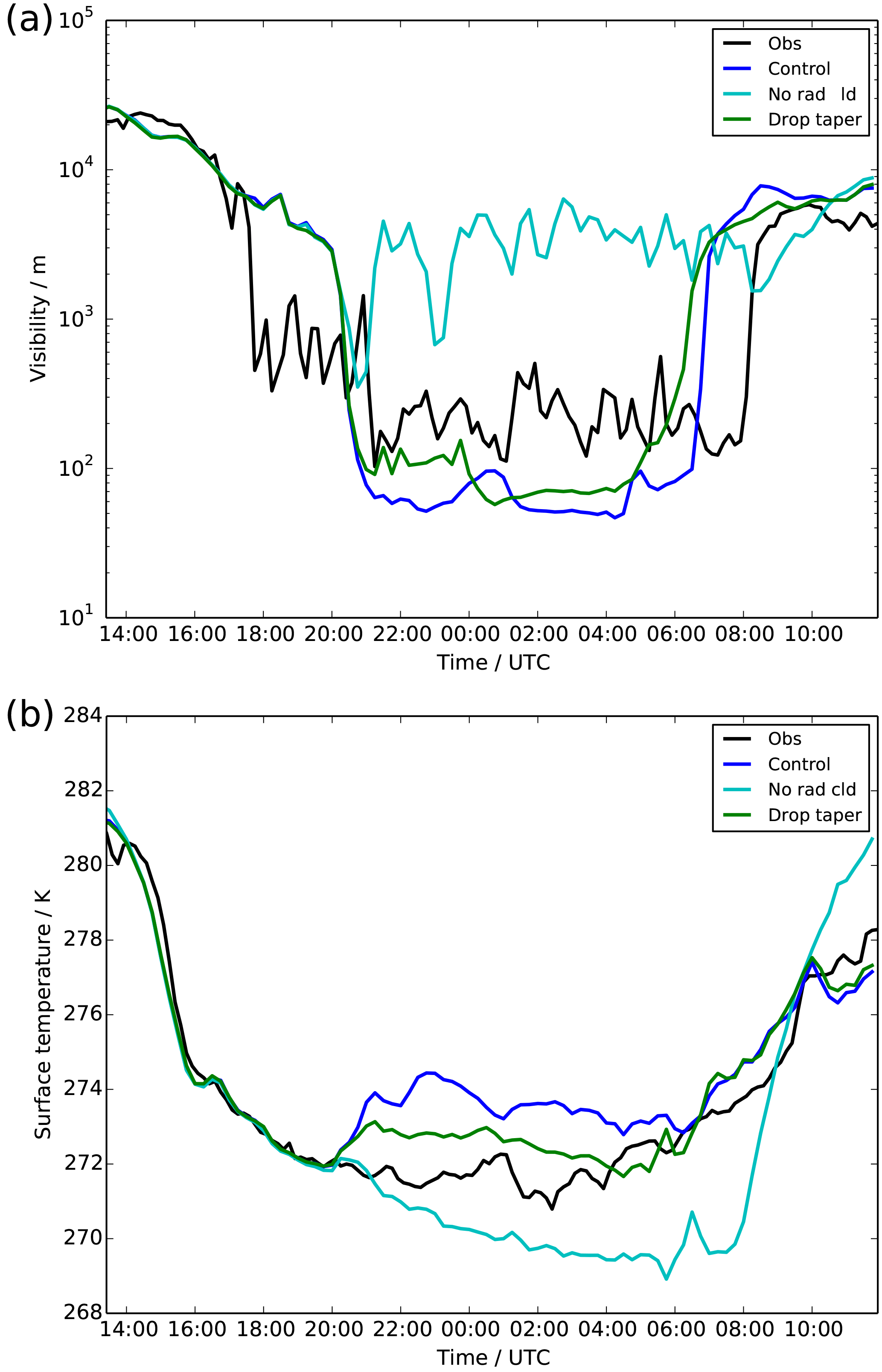
Figure 1Time series of observations (black) and UKV experiments: control (blue), radiatively inactive cloud (cyan) and modified droplet number (green), showing (a) visibility and (b) grass-surface temperature.

Download

The control UKV shows a very good simulation of the pre-fog conditions, tracing the observed surface temperature (Fig. 1b) almost perfectly until the onset of fog at 20:00 UTC. The model then shows a sharp drop in median visibility, down to <100 m, at approximately the same time that the observations show a drop in visibility to similar values. The model also produced non-zero probabilities of visibility <1 km from 18:00 UTC; therefore it appears that the onset of fog, particularly the timing, is reasonably well reproduced in this model. However, after the onset of fog, there are noticeable differences between the model and observations. The model shows a 2 K increase in surface temperature immediately after the onset of fog, something which is not apparent in reality. It also appears that the fog is too thick in the model, with visibilities close to 60 m, compared with 200 m in the observations. The dissipation of fog also occurs about 1–1.5 h too early, although this is due to a bank of mid-level cloud arriving at the location too early in the model. The cloud causes an increase in downwelling long-wave radiation, which directly heats the surface and fog layer, causing its dissipation. In reality, it is difficult to determine whether it was the presence of this cloud or the onset of downwelling short-wave radiation after sunrise (08:00 UTC) which caused dissipation, as both occurred at approximately the same time.

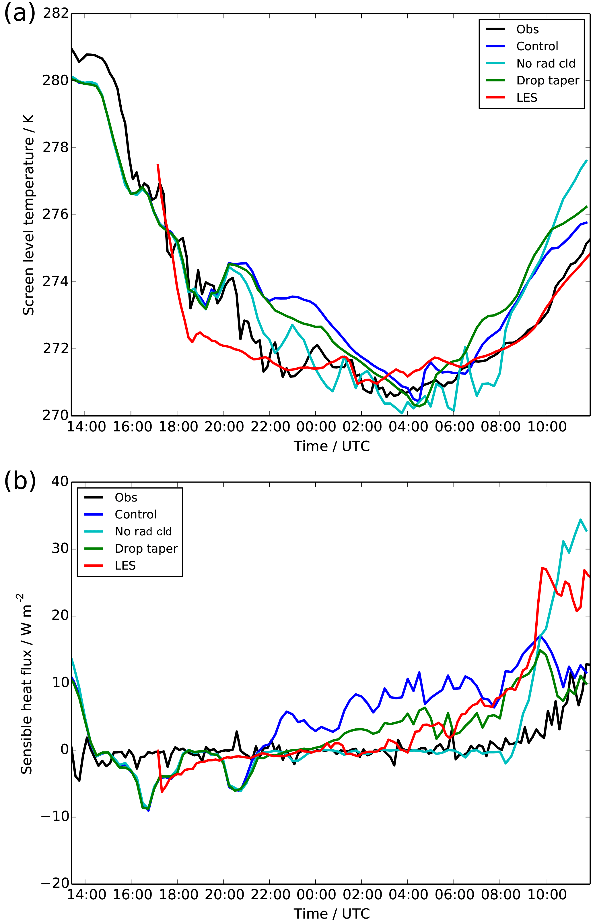
Figure 2Time series of observations (black), LES (red) and UKV experiments: control (blue), radiatively inactive cloud (cyan) and modified droplet number (green), showing (a) screen (1.5 m) temperature and (b) surface sensible heat flux.

Download

Figure 2 shows the screen temperature and surface sensible heat flux from the UKV simulation. The sharp rise in surface temperature after the onset of fog leads to a positive sensible heat flux being formed throughout the night. Although modest in size (10 W m⁻²), it is in clear contrast to the observations which remain near zero throughout, and drives a warming of the screen temperature, which therefore remains warmer than the observations. Figure 3 shows the effect this has throughout the boundary layer. The positive heat flux exists through the lowest 50 m of the atmosphere before dropping to zero at what is likely to be the boundary layer top. The observations, by contrast, show a near-zero flux throughout the depth of the boundary layer. The consequence of this for the temperature profiles is that reality maintains a stable boundary layer, whilst the model has a well-mixed temperature profile indicative of an unstable boundary layer.

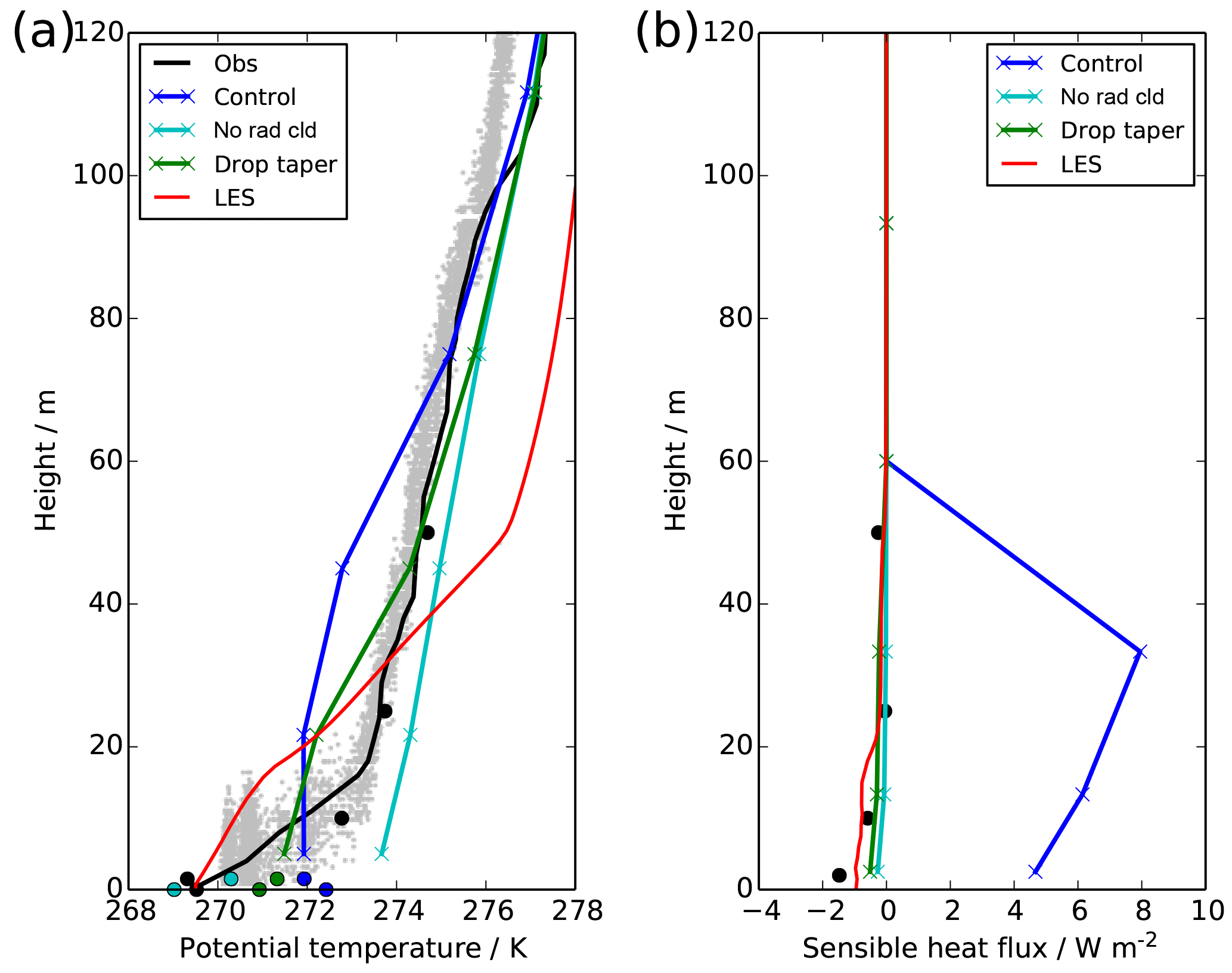
Figure 3Profiles at 22:30 UTC showing observations (mast: black circles, radiosonde: black line, tethered balloon: grey dots), LES (red) and UKV experiments: control (blue), radiatively inactive cloud (cyan) and modified droplet number (green), showing (a) potential temperature and (b) sensible heat flux. Model profiles show model-level data (crosses) and diagnosed screen and surface-level temperature (filled circles).

Download

To understand what is going wrong in the model, it is useful to consider the typical evolution of a real-world radiation fog event, such as this one. Long-wave radiative cooling of the land surface gives rise to a stable boundary layer profile, and a thin fog will form within this profile when the relative humidity reaches 100 %. Initially this fog will only interact weakly with the environment, allowing the surface and air temperature to continue to cool and the fog to thicken. It will take several hours for the fog to start to develop turbulent behaviour of its own. At this point, long-wave radiative cooling from the fog top will generate negatively buoyant air parcels, which will descend throughout the fog layer and generate turbulence. Long-wave emission from the fog layer will also act to heat the surface, which is now “insulated” from the clear sky by the fog layer, and this in turn will maintain its temperature or even allow it to warm, generating a positive surface sensible heat flux. Upward heat flux from the soil is also a significant contributor to surface heating once the surface net radiation has reached near zero (Duynkerke, 1999). The combination of these processes is what leads to the development of a well-mixed fog layer, but this process normally takes many hours. However, the model appears to be simulating this process almost instantaneously – mature, well-mixed fog is formed within an hour of fog onset.

The radiative effect of the fog appears to be a key feature in the process; therefore as a sensitivity test we turn off the radiative effect of any fog which forms in the model (i.e. by setting the absorption and scattering coefficients for condensed water to zero, denoted “No Rad Cld”), shown in Figs. 1–3. The screen temperature and sensible heat flux now show a very good agreement with observations, although the surface temperature is now far too cold and no appreciable fog layer actually forms; i.e. the visibility remains quite high. This demonstrates that the radiative feedback is very important in both the development of the fog and in maintaining the surface temperature. Although fog does form due to the temperature dropping and relative humidity reaching 100 %, the lack of any enhanced radiative cooling from the fog itself prevents further development and thickening of the fog. There are also differences in the temperature structure between the model and observations. The layer of enhanced cooling near the surface is ≈20 m deep in reality, whereas it sits entirely below the lowest model level in the model. This means that the gradient is much sharper, explaining the colder surface temperature for given (and approximately correct) free atmospheric temperatures and screen-level temperature. It is unclear whether this is a consequence of the fog interaction or the model vertical resolution, as discussed in Vosper et al. (2013).

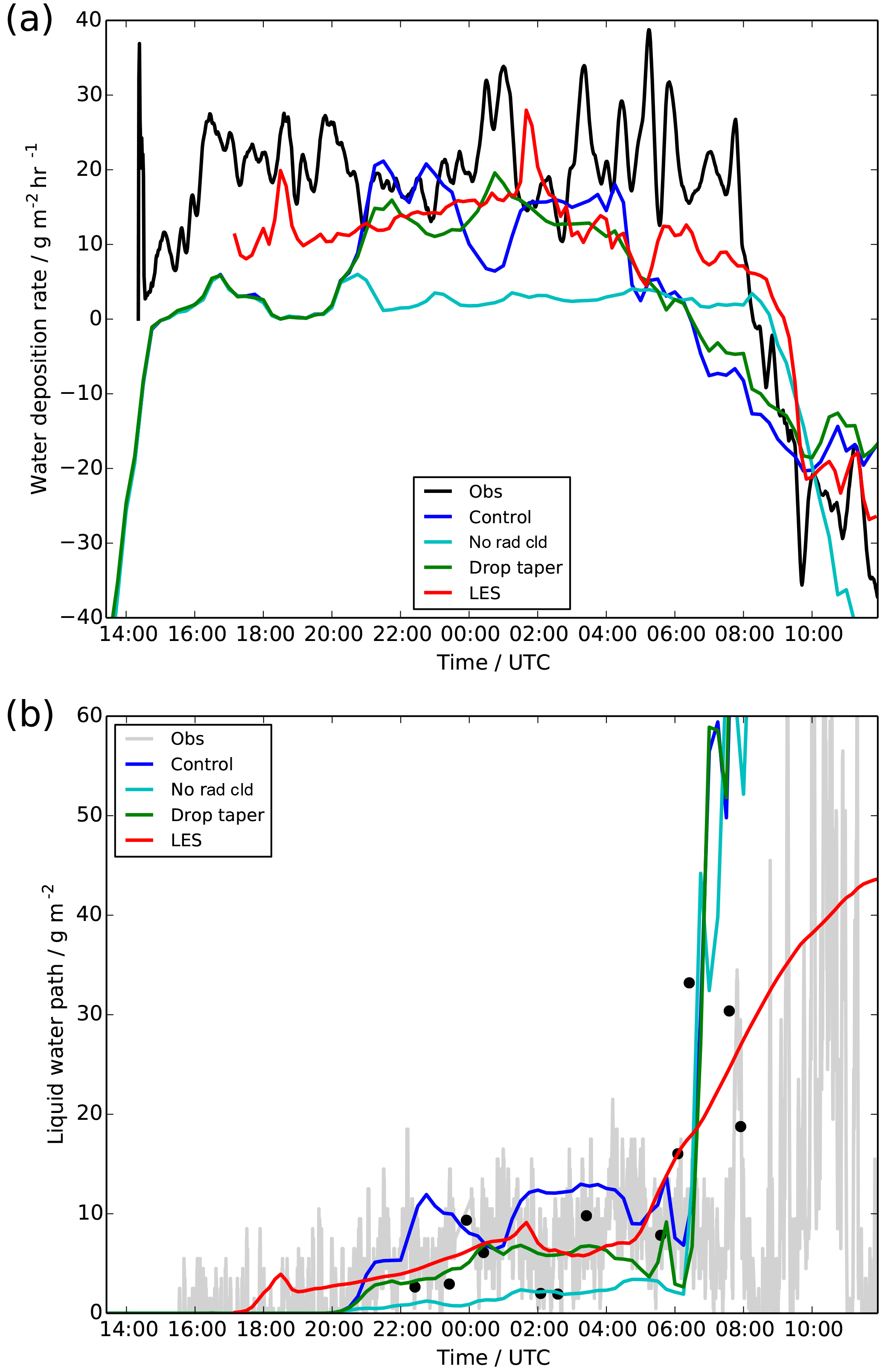
Figure 4Time series of (a) surface water deposition rate, and (b) liquid water path, showing observations (a black; b tethered balloon: black dots, radiometer: grey line), LES (red) and UKV experiments: control (blue), radiatively inactive cloud (cyan) and modified droplet number (green).

Download

Whilst having radiatively inactive fog is clearly unrealistic, the differences in temperature and heat-flux evolution from the control simulation suggests that perhaps the fog is too radiatively active. Guedalia and Bergot (1994) showed that errors in the development of radiation fog can be caused by errors in dew deposition – depositing too little dew onto the surface leaves too much condensed water in the atmosphere, which in turn has too strong a radiative effect. Figure 4a shows observations of dew deposition from the instrument described in Price and Clark (2014) in comparison to the model. During the main period analysed (20:00 to 04:00 UTC) the control simulation is in reasonable agreement with the observations – it is at the lower end of the observational range but certainly within the uncertainty of the instrument. Before 20:00 UTC, the control simulation underestimates the deposition, and this is likely to be due to hygroscopic absorption, a process not accounted for in the model's surface latent heat flux parameterisation, as discussed in Price and Clark (2014). There is also very shallow and inhomogeneous fog present in reality at this time, which is not simulated by the model, as it is only several metres deep and thus below the first model level, but it will contribute to the observed deposition rate. The radiatively inactive fog, by contrast, shows almost no deposition throughout the simulation, and this is due to the fact that no appreciable fog layer forms in the simulation, and the dominant (model) process leading to surface dew deposition is sedimentation of condensed water onto the surface.

Hence the dew deposition may be slightly underestimated in the control simulation, but the effect of this will only become significant if it, in turn, leads to a significant overestimate in the condensed water content. Figure 4b shows the liquid water path (LWP) and Fig. 5a a profile through the fog layer from the tethered balloon. The profile shows the kind of variability which exists in the fog depth and water content and is not indicative of any fog development between the two observation times. The control simulation is in reasonable agreement with the observations for much of the night, although generally at the higher end of observed variability. The radiatively inactive fog is clearly too thin when compared to all available observations. Hence it appears that errors in dew deposition and the evolution of the condensed water content are not the main causes of error in the radiative effect of fog. However, the radiative effect of fog is not only controlled by the liquid water content but also by the number of cloud droplets and therefore their size. Figure 5b shows that the number of droplets observed from the tethered balloon is significantly lower than those predicted by the model.

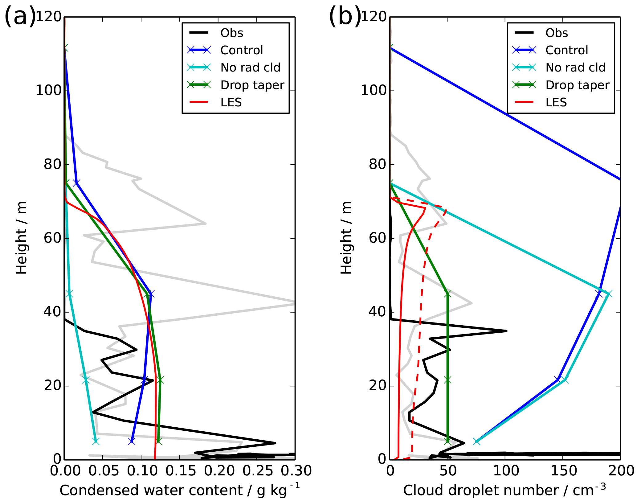
Figure 5Profiles at 00:30 UTC showing observations (00:00 UTC: grey, 00:30 UTC: black), LES (red) and UKV experiments: control (blue), radiatively inactive cloud (cyan) and modified droplet number (green), showing (a) cloud liquid water content and (b) cloud droplet number concentration. For the LES droplet number, we show only the activated droplets (solid) and all particles >2 µm (dashed).

Download

The model parameterisation (Wilkinson et al., 2013) uses a fixed value of 75 cm⁻³ for the droplet concentration at the lowest model level, tapering up to a value determined by the concentration of aerosol (Osborne et al., 2014) at 150 m. This tapering process is a pragmatic attempt at representing the fact that cloud droplet numbers in fog tend to be lower than those observed higher up in the atmosphere (Gultepe et al., 2009; Price, 2011). However, it appears that it is failing to represent some key features. The droplet numbers in fog are believed to be low because, despite the abundance of aerosol near the surface from which cloud droplets could form, the lack of any appreciable updraughts in the near-surface stable boundary layer results in weak supersaturations. This prevents the aerosol from being activated and therefore only relatively few aerosol droplets become hydrated. The observations also show the droplet numbers to be approximately constant throughout the fog layer, whilst the model's (imposed) profile increases quickly with height from its surface value, due to the large value diagnosed higher up from the aerosol concentration.

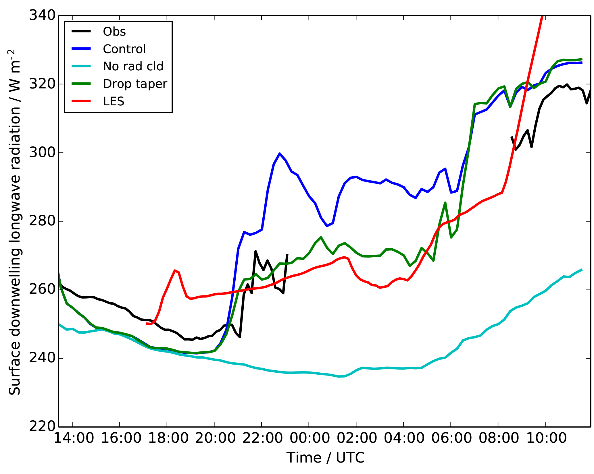
Figure 6Time series of surface downwelling long-wave radiation, showing observations (black), LES (red) and UKV experiments: control (blue), radiatively inactive cloud (cyan) and modified droplet number (green).

Download

The abundance of small cloud drops in the model will increase the cloud absorptivity, making the fog optically thicker and more radiatively important. This will drive stronger radiative cooling from the fog top, enhancing the turbulence and causing the development of well-mixed fog. It will also increase the downwelling long-wave radiation at the surface, which will in turn heat the surface and drive a positive sensible heat flux. However, observations of downwelling long-wave radiation (Fig. 6) are not available for much of the night due to ice formation on the dome of the radiometer rendering the measurements unusable. The initial rise in downwelling long-wave radiation (between 20:30 and 23:00 UTC, before the ice formed) is representative of the fog, and it would not be unreasonable to assume that values remained near 270 W m⁻² throughout the night, perhaps increasing slightly as the fog developed. Therefore the model would appear to have excessive downwelling long-wave radiation, but at this point we shall appeal to the additional information that can be provided by the LES model to support this conclusion.

Figures 2–6 also showed results from the LES, which generally appear to be in good agreement with the observations, demonstrating that the LES is a representative proxy for reality. They also confirm that the low cloud droplet number (Fig. 5b) is responsible for a much lower downwelling long-wave radiation (Fig. 6) than is simulated by the UKV. The LES also provides the opportunity to explore the mechanisms leading to cloud droplet activation (or lack thereof) in the fog and therefore to suggest improvements to the NWP model.

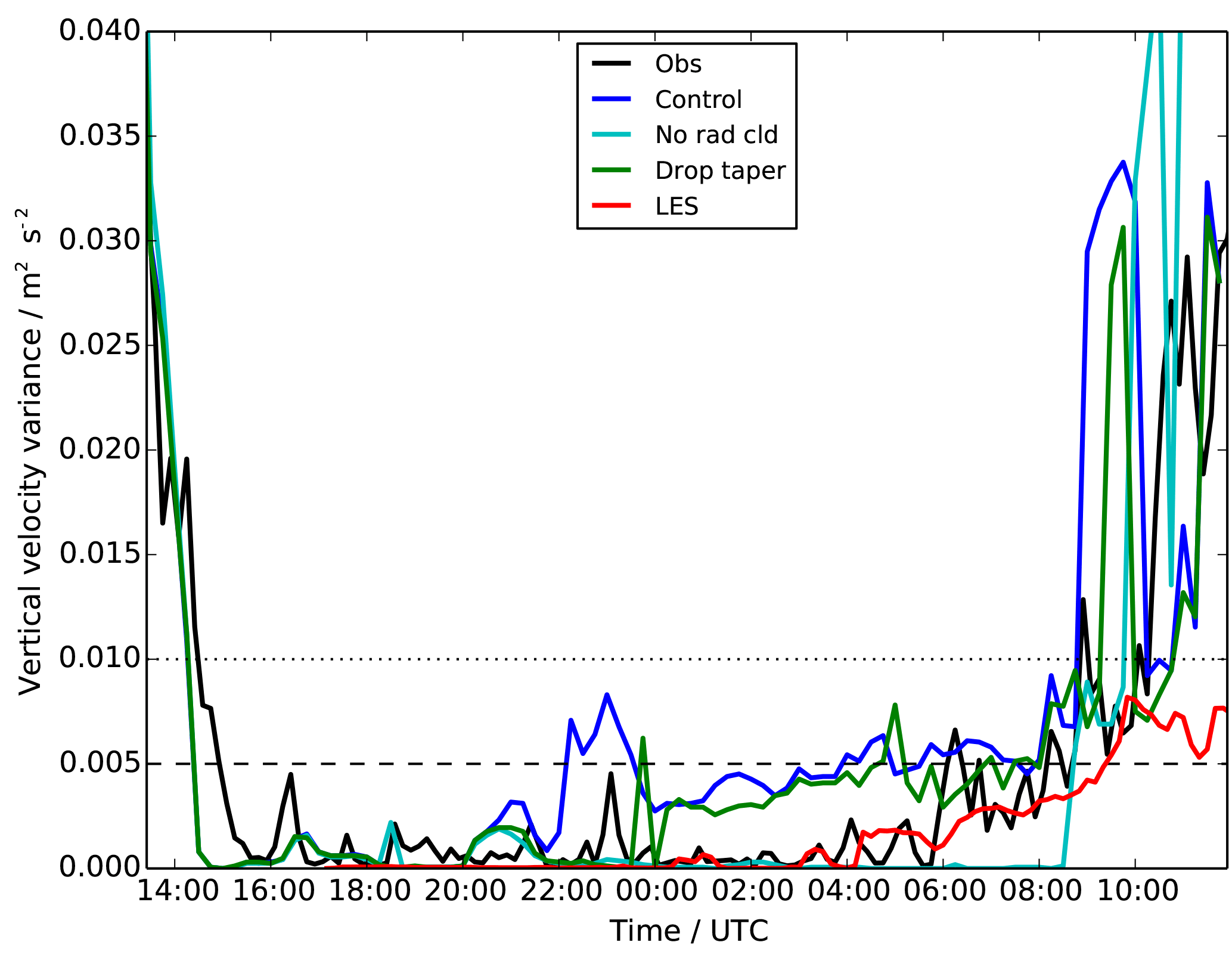
Figure 7Time series of vertical velocity variance at screen level (2 m), showing observations (black), LES (red) and UKV experiments: control (blue), radiatively inactive cloud (cyan) and modified droplet number (green). Also shown are the Price et al. (2018) value above which fog will not form (dashed) and the minimum value used in most activation parameterisations (dotted).

Download

Figure 7 shows the near-surface vertical velocity variance, which is very low in the observations and all models. Indeed it is safely below the 0.005 m² s⁻² suggested in Price et al. (2018) for the threshold value above which fog will not form. What this implies is that the peak updraught speed driving aerosol activation is very low, typically <0.1 ms⁻¹. This is much lower than the typical updraught speeds found in “normal” clouds (i.e. those which do not contain a rigid surface at their lower boundary). Because most models do not prognose or diagnose supersaturation, most aerosol activation parameterisations (e.g. Ghan et al., 1997; Morrison and Gettelman, 2008; West et al., 2014) link this updraught speed directly to the number of activated droplets. However, these parameterisations were not developed in the weak updraught regime of radiation fog, instead typically imposing a minimum updraught velocity or standard deviation of 0.1 ms⁻¹ or higher. Therefore, if any schemes like this are used to simulate aerosol activation in fog, they will systematically overestimate the amount of aerosol activation and therefore the cloud droplet number, with inevitable consequences such as those discussed in Sect. 3.

For fog formation, updraughts are obviously not the only process that will activate aerosol and lead to the formation of cloud droplets. The fundamental process which drives activation is the ambient supersaturation, driven by adiabatic cooling, which can be driven by updraughts but in fog is also driven by direct cooling of the atmosphere. The observed cooling rate during the first few hours of fog formation (Fig. 2a) is 1 K h⁻¹, which would be equivalent to an updraught speed of 0.04 ms⁻¹ assuming a temperature lapse rate of 6.5 K km⁻¹. This is still significantly below the 0.1 ms⁻¹ minimum used for aerosol activation (even when added to the observed turbulent vertical velocities), demonstrating that typical parameterisations do not even indirectly represent the physical processes or amount of aerosol activation correctly. Further work is clearly warranted to develop schemes which are appropriate for this regime.

Figure 8Time–height contour plot from the LES showing water vapour supersaturation with respect to the saturation vapour pressure over liquid water.

Download

Figure 8 shows the supersaturation as predicted by the LES throughout the simulation. The first point to note is that the values are very low, <0.1 %, which is much lower than values typically found in clouds (0.3–1 %, Ghan et al., 1997; 0.2–1.5 %, Spracklen et al., 2011). Low supersaturation values are also supported by earlier observations in different fog campaigns. For example, in the ParisFog campaign in France, the maximum effective supersaturation was found to be less than 0.05 %, with the average activation diameter of particles between 350 and 450 nm (Hammer et al., 2014). Similar findings were also obtained in the Po Valley, Italy, highlighting the role of aerosol chemical composition (Gilardoni et al., 2014).

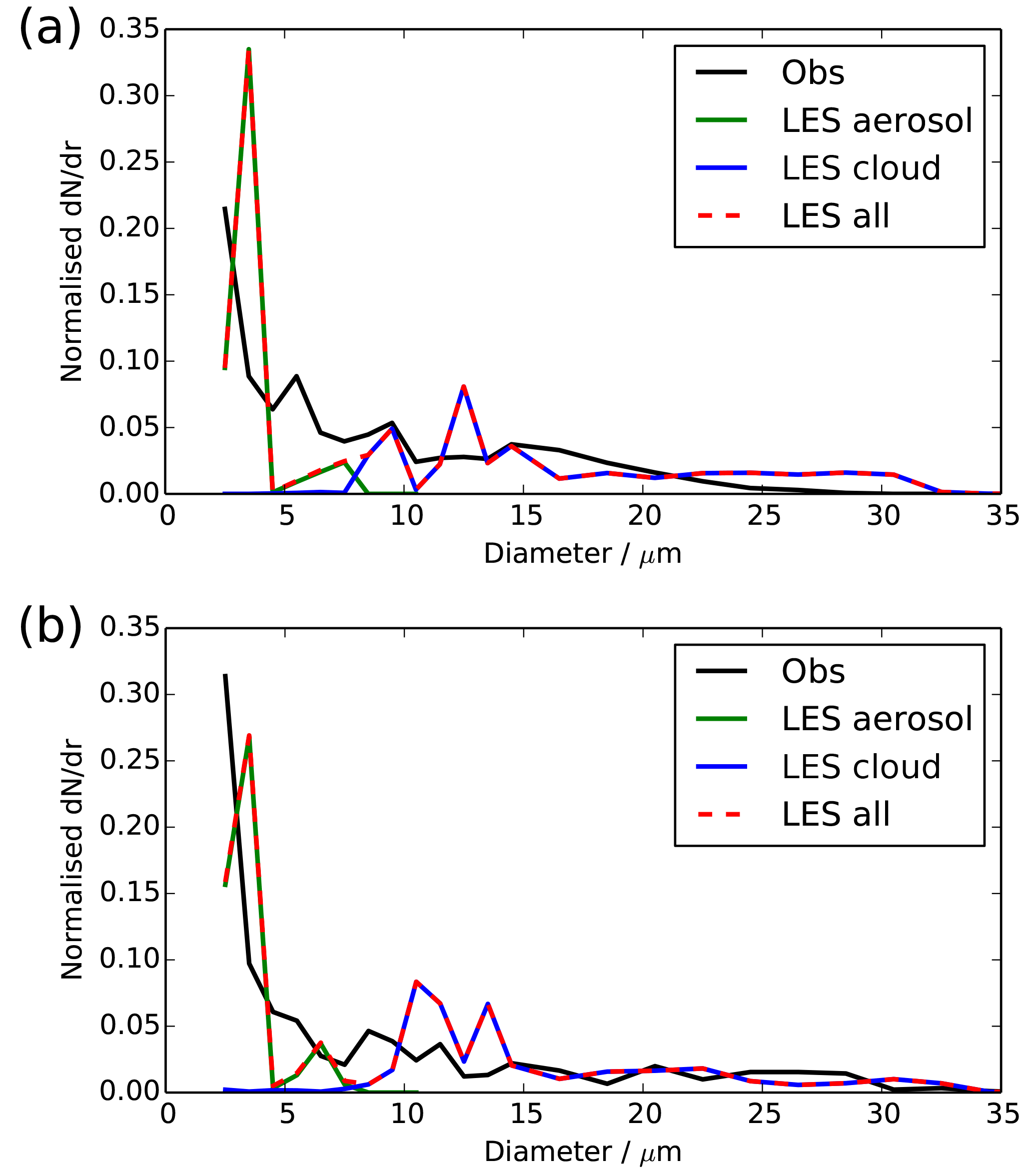
Figure 9Cloud droplet size spectra at (a) 00:30 UTC and (b) 03:30 UTC, showing observations (black) and LES (red). For the LES, we also show the number of activated drops (blue) and number of aerosol particles (green).

Download

These low supersaturation values explain the very low levels of aerosol activation and therefore low cloud droplet number values. Figure 9 shows the size spectra of particles >2 µm, which shows that there are large numbers of very small particles (<5 µm) in both the observations and LES. It is likely that these particles are not activated cloud drops, but large aerosol particles which have absorbed water and swollen in size. We note here that we have excluded the lowest (1–2 µm) bin of the cloud droplet probe from our analysis to avoid potential noise issues with large, dry aerosol affecting the numbers. Because of the low supersaturation and therefore high activation diameter, hydrated aerosol particles within fog can grow larger than micrometre in size and can contribute up to 68 % of total light scattering during different fog periods (Hammer et al., 2014; Elias et al., 2015). However, most of these hydrated particles are still too small to considerably affect interaction with long-wave radiation after fog has developed. This explains how the visibility can become so low, and yet the fog remains optically thin and the boundary layer stable.

The LES allows us to analyse this further, because we can break the size spectra into their contributions from hydrated particles which are still in the LES aerosol classes and particles which have been activated into the LES cloud droplet classes, i.e. exceeded the critical size given by Köhler theory. As shown in Fig. 9, almost all particles in the LES with diameter <6 µm are wet aerosol, and only those with diameter >6 µm are activated cloud drops. This distinction can also be seen in profiles of the cloud droplet number (Figs. 5b and 10b), where we have shown both the LES results for all particles >2 µm (as measured by the cloud droplet probe) and only those which are activated cloud drops. There is approximately a factor of 2 difference between these two estimates of cloud droplet number, with the all-particle estimate comparing best with the observations. In the simulation, aerosol is assumed to be composed of ammonium sulfate, which might be more hygroscopic than the actual aerosol observed during IOP1. Less hygroscopic aerosol would have a lower growth factor within fog, and thus the transition from hydrated aerosol to activated fog droplets would be seen at a smaller diameter. However, less hygroscopic aerosol would also activate less efficiently, thus increasing the critical dry diameter of activating particles. Thus we are confident that the small droplets seen in the observations are not fully activated but are significantly hydrated aerosol. This suggests that many observational estimates of fog droplet number, particularly in clean air masses, could actually be overestimating the number of activated droplets (i.e. those that are radiatively important in the long wave).

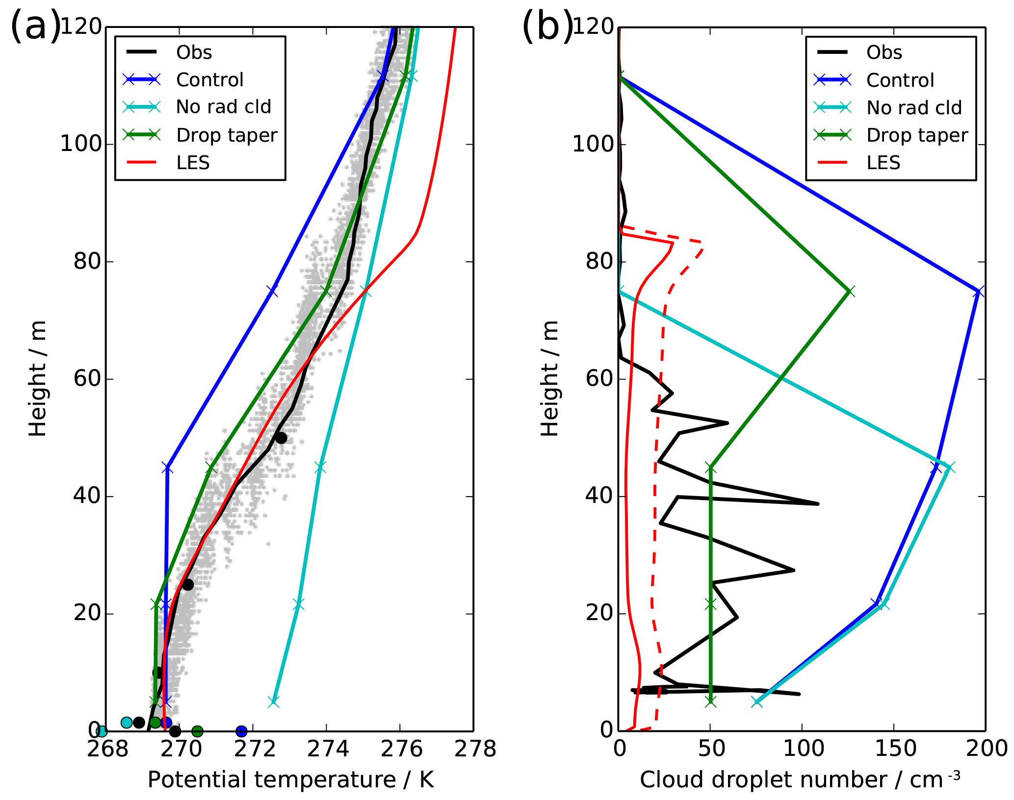
Figure 10Profiles at 03:30 UTC showing observations, LES (red) and UKV experiments: control (blue), radiatively inactive cloud (cyan) and modified droplet number (green), showing (a) potential temperature and (b) cloud droplet number concentration. Model profiles show model-level data (crosses) and diagnosed screen and surface-level temperature (filled circles). For the LES droplet number, we show only the activated droplets (solid) and all particles >2 µm (dashed).

Download

The supersaturation and turbulence levels remain remarkably constant throughout the night (up to 04:00 UTC), resulting in a cloud droplet number concentration which also remains reasonably constant throughout the night (Figs. 5b and 10b). This implies that the downwelling long-wave radiation (and optical depth) of the fog is mainly driven by its physical depth, which grows throughout the night (see Fig. 8). The growth of the fog layer leads to a gradual but continuous increase in the downwelling long-wave radiation throughout the night (Fig. 6), with the exception of a small decrease around 02:00 UTC. This occurs because of a sharp decrease in the background specific humidity (not shown) at around 80 m, and therefore the fog growth is temporarily inhibited due to the entrainment of this drier air. This gradual rise in the downwelling long-wave radiation is responsible for the surface temperature ceasing to cool by 02:00 UTC and slowly warming throughout the rest of the night, which in turn drives a slow transition towards a well-mixed fog layer.

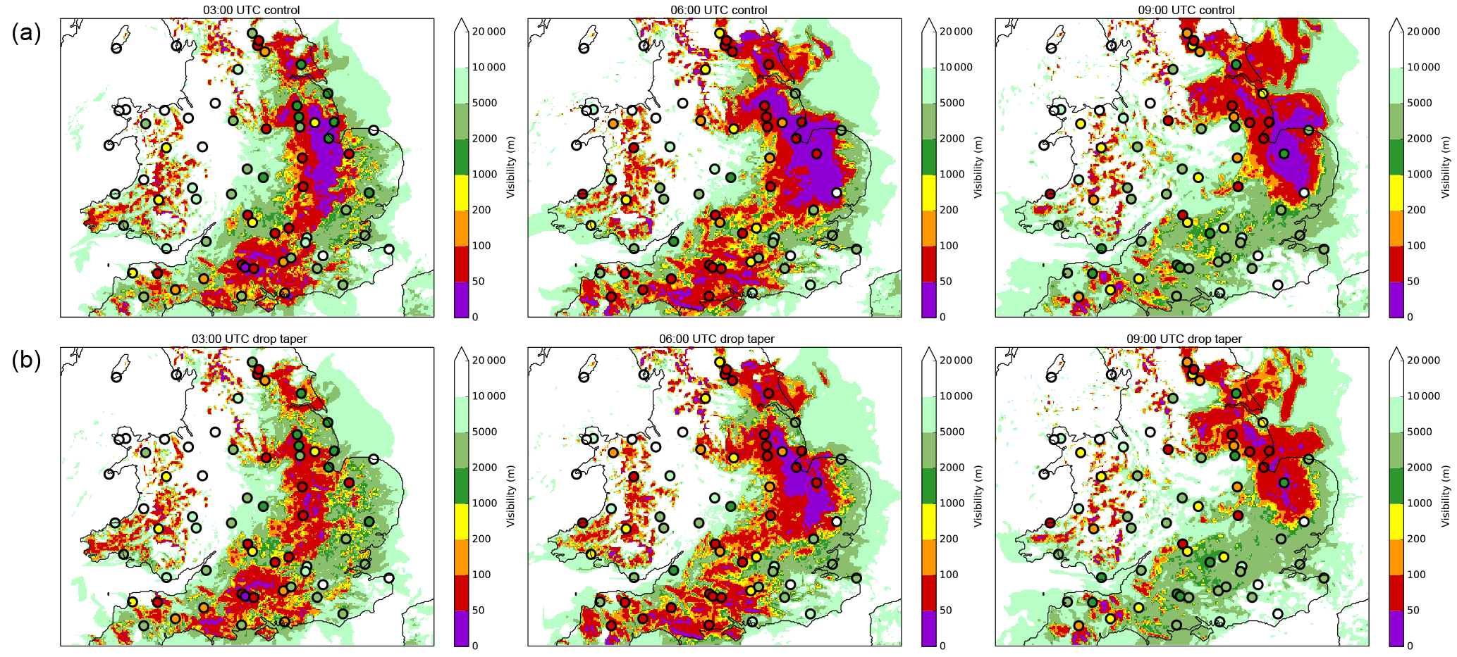
Figure 11Visibility forecasts from 00:00 UTC on 10 February 2015 at 3 h intervals from the UKV control (a) and with modified droplet number (b). Filled circles show observations.

Download

Figure 10 shows that by 03:30 UTC, the surface is warmer than the near surface and the lowest 20 m of the atmosphere is well mixed, with the top portion of the fog layer remaining stable. It is interesting to note that once the fog becomes adiabatic, the mixed layer temperature is very similar to that predicted by the control NWP model, although the NWP model mixed layer is much deeper because it has been developing for many hours. This can also be seen by the convergence of screen temperature in all models around 04:00 UTC in Fig. 2a. After this time, the updraught speeds within the fog begin to grow, leading to increased droplet activation and a rise the observed and LES cloud droplet numbers. Figure 9b shows a small secondary peak in the size spectra around 10 µm, developing due to the increasing turbulence, and the evolution of the spectra and cloud droplet numbers after this point is very similar to that already reported in Price (2011) and Tonttila et al. (2017); hence we do not focus on it here. The well-mixed layer continues to grow throughout the night, until the entire fog layer is well mixed and turbulent by 08:00 UTC.

To test whether improving the representation of aerosol activation would improve the simulation of fog in the NWP model, we make a simple adjustment to the cloud droplet profile used in the UKV (denoted “Drop Taper”). Instead of tapering from a fixed value (75 cm⁻³) at the surface to the aerosol-dependent value at 150 m, we keep the droplet number fixed throughout the lowest 50 m of the atmosphere, before tapering towards the aerosol value above this. This is motivated by the observations and LES results, which show that the cloud droplet number is reasonably uniform throughout the fog layer. We also reduce the fixed value used in the lowest 50 m to 50 cm⁻³, which is more representative of the observations, although still possibly too high. Clearly this choice is likely to be location and case specific and requires some adjustments for more polluted locations as discussed in Jayakumar et al. (2018). A universal parameterisation would require some link to aerosol.

Figures 1–7 and 10 show the results from this simulation and demonstrate that improvement is possible. The downwelling long-wave radiation (Fig. 6) now remains much lower throughout the night, which allows the surface to remain cool and the sensible heat flux to remain near zero (Fig. 2). The model can maintain a stable atmospheric temperature profile for the early part of the night (Fig. 3a), and eventually it transitions to a well-mixed profile (Fig. 10a). Therefore, it would appear that by having a realistic estimate of cloud droplet numbers in fog we can significantly improve NWP fog simulations.

The mechanisms by which this improvement occur are twofold. Firstly, the reduced cloud droplet number increases the bulk sedimentation rate, which is calculated via Stokes Law (Wilkinson et al., 2013). This increases the rate at which condensed water is removed from the fog layer onto the surface, physically thinning the fog layer, i.e. the LWP is reduced. This is shown in Fig. 4, where the LWP is approximately halved, yet the water deposition rate (which is almost entirely droplet settling) is largely unchanged. Secondly, the increased effective radius, which comes from reducing the cloud droplet number, reduces the cloud absorptivity to upwelling long-wave radiation (Slingo and Schrecker, 1982). This allows more radiation to be emitted to space, reducing the effectiveness of the fundamental process by which radiation fog develops – long-wave emission from the fog itself (Fig. 6), which is proportional to the absorption. Cooling from the fog top is less efficient at turbulence production, and downwelling long-wave radiation from the fog is less efficient at heating the surface (and thus enabling surface-driven turbulence to form). Both of these processes inhibit the transition to well-mixed fog. The radiatively inactive cloud experiment is an extreme example of this effect.

Given the simple nature of the aerosol representation in the UKV and the current method of calculating cloud droplet numbers from this, the solution proposed above may actually be a suitable candidate for operational NWP implementation over the UK. To evaluate this, we run a month-long trial of the full data assimilation and forecast system for February 2015 with four forecasts per day (00:00, 06:00, 12:00, 18:00 UTC), each 36 h in length. This represented a typical UK winter, comprising periods of high pressure with calm, potentially foggy conditions, and periods of westerly flow bringing low-pressure frontal systems across the country. The headline result is a small improvement across all measures of forecast skill (wind speed, temperature, cloud cover, precipitation, visibility). One of the more interesting changes was a non-negligible improvement in screen temperature forecasts. Despite the fact that there were only relatively few foggy days during the month, the screen temperature error (similar to Fig. 2a) is so great when fog is present, that improvements to this can be seen in the mean temperature error across the entire month.

The main improvements, however, are seen in surface visibility forecasts, such as those shown in Fig. 11. The figure shows a widespread fog event over central and southern England on 10 February 2015. The fog onset occurs around 01:00 UTC in the observations, and both forecasts reproduce this reasonably well. However, once the fog is formed in the control simulation, it is instantly thick, well-mixed fog with visibilities <50 m, symptomatic of the problems discussed in Sect. 3. This is not observed in reality, with many stations reporting visibilities nearer to 100 m. The control simulation maintains these low visibilities throughout the night as the fog moves across the country. By 09:00 UTC, the fog is dissipating in most places in reality, whilst the model retains a large area of thick fog with very low visibility.

With the revised droplet taper, the onset and dissipation phases of the fog event are improved. The fog onset is slower, with visibilities around 100 m forecast at 03:00 UTC, in general agreement with the observations. By 06:00 UTC, the fog has thickened, becoming well mixed and with visibilities in places falling below 50 m. Whilst this is still too thick compared to the observations, it is certainly much better than the control. By 09:00 UTC, the fog has started to dissipate in the model, with visibilities rising, again in better agreement with the observations.

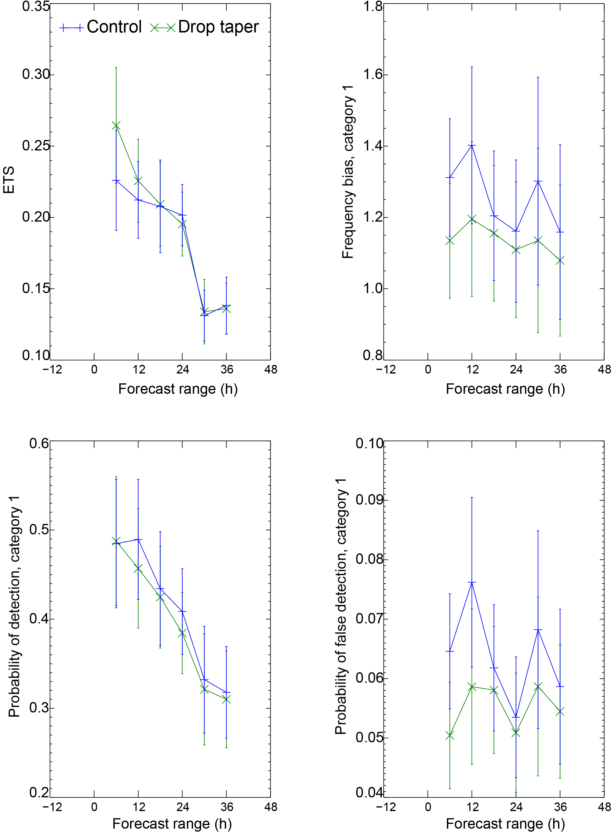
Figure 12NWP model verification of visibility from 5 February to 5 March 2015 utilising all observations and forecasts (4 per day) over UK land areas. Panels show the equitable threat score (ETS), frequency bias, probability of detection and probability of false detection, for a visibility threshold of 200 m, from the UKV control (blue) and with modified droplet number (green).

Download

Figure 12 provides more quantitative support for these conclusions, presenting categorical verification of all forecasts in the trial period against all available surface observations. Following Mason (2003), we define a 2 × 2 contingency table such that a is the number of hits, b is the number of false alarms, c is the number of misses and d is the number of correct negatives. We then determine the equitable threat score (ETS) as $(a-X)/(a-X+b+c)$ where $X=(a+b)(a+c)/(a+b+c+d)$, the frequency bias as $(a+b)/(a+c)$, probability of detection (hit rate) as $a/(a+c)$ and the probability of false detection (false alarm rate) as $b/(a+b)$. Perfect scores are 1 for the ETS, frequency bias and probability of detection, and 0 for the probability of false detection. In Fig. 12 we consider the 200 m threshold for visibility, although results are similar at other thresholds (e.g. 1 km). As shown, the control simulation was overforecasting low-visibility events, with a frequency bias >1 and a probability of false detection >0. Including the modified drop taper has clearly improved both of these metrics. Importantly, it has done this without significantly degrading the probability of detection, which remains largely unchanged, and therefore the ETS is improved. These results are consistent with the main results from IOP1 and the case study from this trial period is presented in Fig. 11. The control simulation produces fog which is too thick, too fast and tends to persist for too long; i.e. it overforecasts. By improving the droplet numbers, this behaviour is improved and can be seen in the statistical analysis.

Therefore, although not a panacea, the changes presented here certainly present a useful improvement in fog modelling and highlight that an accurate representation of aerosol and its interaction with fog are key challenges for NWP. Future work should look to link the near-surface droplet number to aerosol for a more complete and globally universal solution.

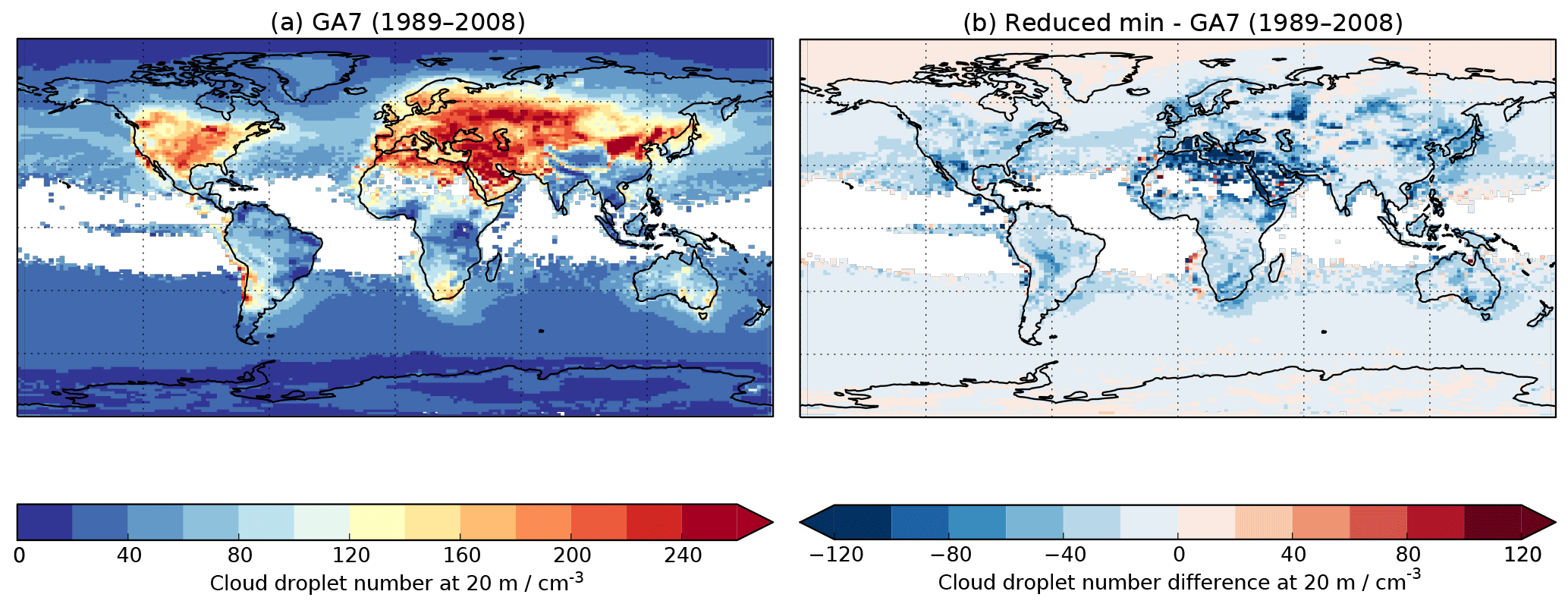
Figure 13(a) 20-year mean cloud droplet number concentration at the lowest model level (20 m) from an atmosphere only simulation of HadGEM3-GA7. (b) The difference from this when reducing the minimum updraught speed used for aerosol activation from 0.1 to 0.01 ms⁻¹.

Download

All data used in this study are available from the authors upon request.

The authors declare that they have no conflict of interest.