2.1 Model setup and data

The data used in this study were obtained from a recent regression-based RSM study conducted in the Beijing–Tianjin–Hebei (BTH) region in China. One baseline scenario and 1100 brute-force controlled scenarios were performed using the Community Multiscale Air Quality Modeling System (CMAQ) (version 5.0.1) in a 12 × 12 km domain over the BTH region. We used the same meteorological conditions for those multiple scenarios and only the emissions were changed in different scenarios. The details of the Weather Research and Forecasting–CMAQ model and emissions were described in a previous study (Zhao et al., 2016). We used the SAPRC99 gas-phase chemistry module (Carter, 2003) and the sixth-generation CMAQ aerosol model (AERO6) (Appel et al., 2013) with the treatment of organic aerosols replaced with the 2D-VBS (two-dimensional volatility basis set) framework (Zhao et al., 2015b, 2017). The simulation period is January and July in 2014 to represent winter and summer, respectively. The emission data were developed by Tsinghua University based on a bottom-up method with a high spatial and temporal resolution (Zhao et al., 2016).

The responses of O₃ (daily 1 h maxima) and PM_2.5 (daily 24 h average) to the emissions of five groups of precursors, namely NO_x, SO₂, NH₃, VOC + intermediate VOC (denoted as “VOCs”) and primary organic aerosol (POA) from five regions, namely Beijing, Tianjin, northern Hebei (denoted as “HebeiN”), eastern Hebei (denoted as “HebeiE”) and southern Hebei (denoted as “HebeiS”) were analyzed. The O₃ and PM_2.5 concentrations were analyzed in urban areas of prefecture-level cities in the five target regions (Zhao et al., 2017). The performance of the model system was evaluated in our previous paper (Zhao et al., 2017; Xing et al., 2017a), which suggested acceptable CMAQ model performance that meets the recommended benchmark in the comparison with ground-observed concentrations, as well as acceptable performance of the regression-based RSM with mean normalized errors within 3 %.

In the regression-based RSM developed previously, the system supports the investigation of different emission changes for five precursors in five regions (i.e., extended RSM, ERSM described in Zhao et al., 2015a and Xing et al., 2017a). In this study, for simplification, the pf-RSM was built on the simultaneous change in one or all regions (i.e., controls separately in an individual region, or jointly controls in all five regions with the same control ratio). However, the pf-RSM can be extended to pf-ERSM following the same structure as the regression-based ERSM but using polynomial functions for PM_2.5, O₃ and precursors.

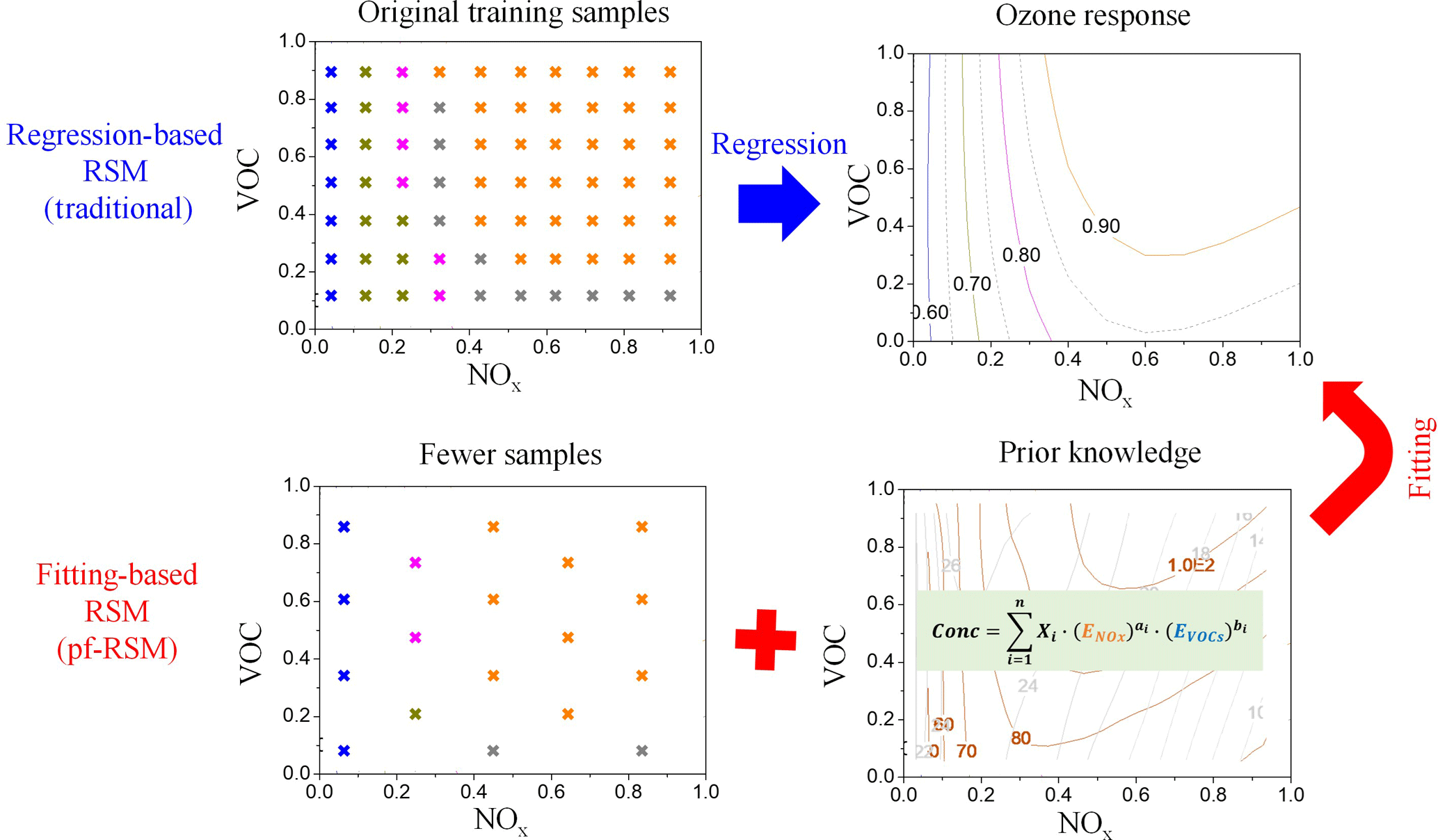
Figure 1Schematic plot of comparison between the traditional RSM (regression-based) and the RSM with a polynomial function (denoted as “pf-RSM”, fitting-based).

Download

2.2 Development of the pf-RSM

In general, tropospheric O₃ and PM_2.5 concentrations are contributed to by its sources and sinks through a series of atmospheric processes, such as horizontal or vertical advection and diffusion, gas-phase chemistry, and deposition. The nonlinear behavior in each of these processes contributes to the nonlinearity in the responses of concentrations to precursor emissions. Similar responsive functions can be expected across regions and time. For example, a universal ozone isopleth diagram developed using the empirical kinetic modeling approach of the U.S. Environmental Protection Agency (Gipson et al., 1981) represents the general O₃ responsiveness to NO and VOC concentrations. A fitting-based model was developed to simplify the O₃ responsiveness to precursor emissions by using a general formulation (Heyes, et al., 1996). The simplified formulation of concentrations to emissions can be easily applied to optimize control strategies (Heyes et al., 1997), which is a great advantage over the regression-based model. Moreover, with the fitting-based RSM, the inclusion of a prior knowledge of pollutant responses to emissions might substantially reduce the case number required to build the RSM (see Fig. 1).

In this study, the prior knowledge of pollutant responses to emissions was characterized as a series of polynomial functions by the previous developed regression-based RSM. The accuracy of the regression-based RSM in representing the nonlinearity in pollutant response to emissions has been examined thoroughly using different methods including cross validation, out-of-sample validation and isopleth validation in previous studies (Xing et al., 2011, 2017a; Wang et al., 2011; Zhao et al., 2015, 2017). The relationship among pollutant responses to emissions followed by the basic chemical functions and physical laws is implicitly represented in the regression-based RSM. In this study, however, we adopted a linear combination of polynomial bases (i.e., 1, x, x², x³…) to explicitly parameterize the pollutant responses to emissions. The coefficients of the function were estimated by fitting the function with training samples selected brute-force to match with the regression-based RSM prediction (i.e., isopleth validation) and the CMAQ simulations (i.e., out-of-sample validation). The flow scheme of the development of the pf-RSM is displayed in Fig. 2. The structure of the polynomial function to be fitted is expressed as follows:

where ΔConc is the response of O₃ and PM_2.5 concentrations (i.e., change to the baseline concentration), and the concentration value can be hourly, monthly or annual averages at either a single grid cell or aggregated grids in the target region; $E_{{\mathrm{NO}}_x}$, $E_{{\mathrm{SO}}_{\mathrm{2}}}$, $E_{{\mathrm{NH}}_{\mathrm{3}}}$, E_VOCs and E_POA are the change ratios of NO_x, SO₂, NH₃, VOCs and POA emissions, respectively, related to the baseline (i.e., baseline = 0); $a_i,b_i,c_i,d_i$ and e_i represent the nonnegative integer powers of $E_{{\mathrm{NO}}_x}$, $E_{{\mathrm{SO}}_{\mathrm{2}}}$, $E_{{\mathrm{NH}}_{\mathrm{3}}}$, E_VOCs and E_POA, respectively; X_i is the coefficient of the term i. ΔConc is calculated from a polynomial function of five variables ($E_{{\mathrm{NO}}_x}$, $E_{{\mathrm{SO}}_{\mathrm{2}}}$, $E_{{\mathrm{NH}}_{\mathrm{3}}}$, E_VOCs, E_POA). The number of terms (n), coefficients (X_i) and degrees (a_i, b_i, c_i, d_i, e_i) of each term were determined using the following steps.

2.2.1 Degree examination

First, the degrees of the five variables were determined individually by fitting the responsive function with a polynomial of a single indeterminate plot (Fig. 3). The PM_2.5 responses to the change in each precursor emission estimated using the RSM were fitted by a series of polynomials of a single indeterminate plot with different orders from the first (linear) to the fifth degree, as shown in following functions (similar to Eq. 1):

$$\begin{array}{}\text{(2)}& {\displaystyle }\mathrm{\Delta }\text{Conc}=\sum _{i=\mathrm{1}}^a{A}_i\cdot {\left(E_{\text{P}}\right)}^i,\end{array}$$

where ΔConc is the response of O₃ and PM_2.5 concentrations to changes in individual precursor emissions; E_P is the change ratio of one precursor (the subscript “P” can represent NO_x, SO₂, NH₃, VOCs or POA) emission related to the baseline; A_i is the coefficient of term i; and the superscript a is the degree of precursor P, which determined the order of the best fitting polynomials.

Table 1Degree of variables in the polynomial function of response to emission changes.

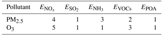
^* $E_{{\mathrm{NO}}_x}$, $E_{{\mathrm{SO}}_{\mathrm{2}}}$, $E_{{\mathrm{NH}}_{\mathrm{3}}}$, E_VOCs and E_POA is the change ratio of NO_x, SO₂, NH₃, VOCs and POA emissions, respectively.

Download Print Version | Download XLSX

Figure 2Flow scheme of pf-RSM development.

Download

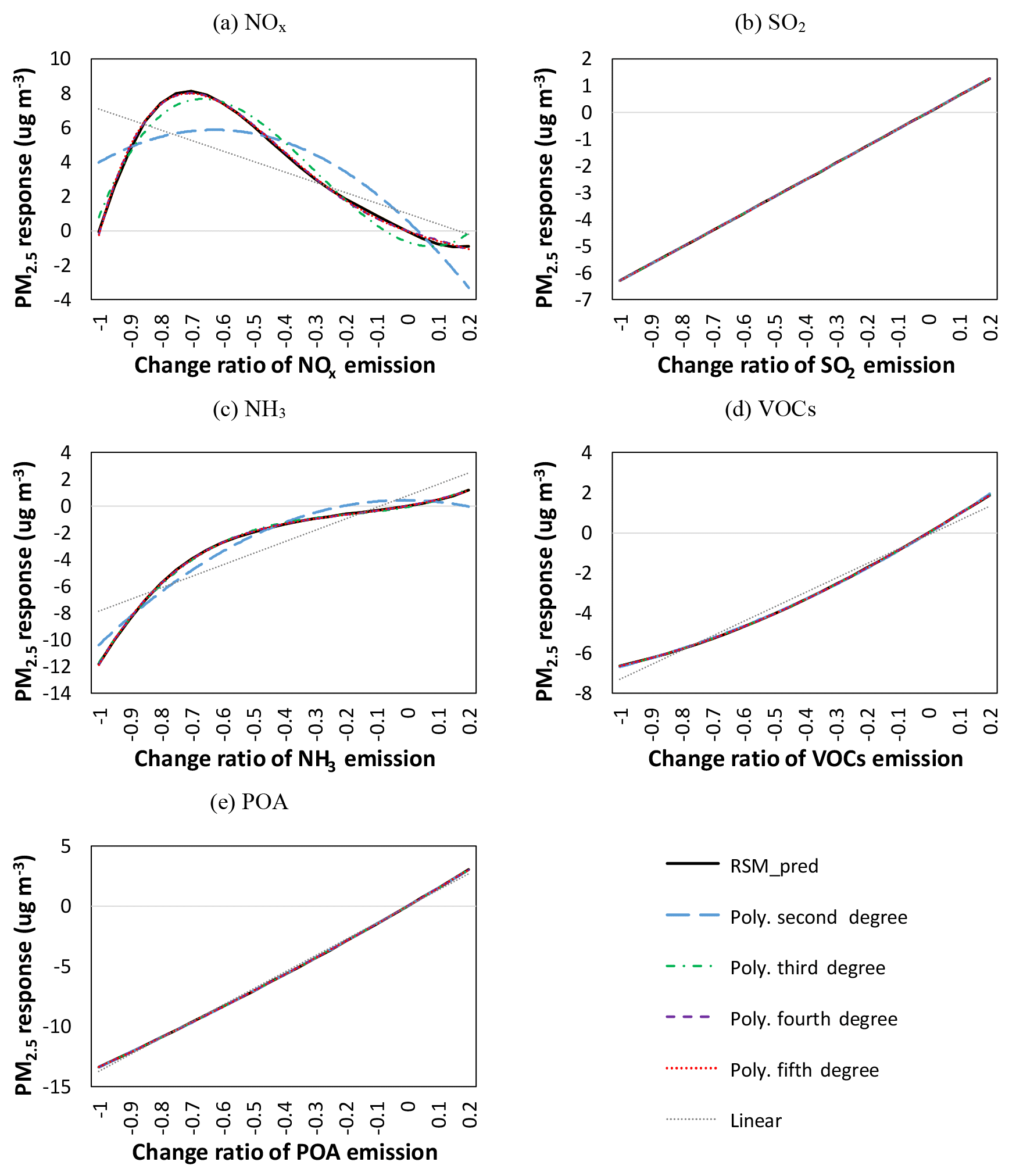
Figure 3Fitting the PM_2.5 responsive function with a polynomial of a single indeterminate plot.

Download

Figure 3a presents PM_2.5 responses to changes in NO_x, showing that PM_2.5 responses cannot be well fitted with polynomials of the order lower than 3. Better performance is shown in fitting with a fourth-order polynomial (R = 0.999, MeanFE = 0.2) than with a third-order polynomial (R = 0.987, MeanFE = 0.6). Thus the degree of NO_x to PM_2.5 should be 4. By contrast, PM_2.5 responses to changes in SO₂ (Fig. 3a) can be well fitted linearly; thus, the degree of SO₂ to PM_2.5 is 1. The degrees of five precursors to O₃ and other pollutants were also examined, and the results are summarized in Table 1. Highly nonlinear responses were found for both O₃ and PM_2.5 to the NO_x, VOC and NH₃ emissions. That might be associated with the strong nonlinearity in the atmospheric oxidation reactions and aerosol thermodynamics which are parameterized with the SAPRC99 gas-phase chemistry module and the AERO6 with 2D-VBS module, respectively, in CMAQ used in this study.

2.2.2 Term selection

The correlation among variables (i.e., product term) was determined in pairs by fitting the responsive function with a polynomial of a two-indeterminate isopleth, expressed as follows:

$$\begin{array}{}\text{(3)}& {\displaystyle }\mathrm{\Delta }\text{Conc}=\sum _{i=\mathrm{1}}^b{B}_i\cdot {\left(E_{{\text{P}}_{\mathrm{1}}}\right)}^{a_i^{\mathrm{1}}}\cdot {\left(E_{{\text{P}}_{\mathrm{2}}}\right)}^{a_i^{\mathrm{2}}},\end{array}$$

where ΔConc is the response of O₃ and PM_2.5 concentrations to changes in individual precursor emissions; $E_{{\text{P}}_{\mathrm{1}}}$ and $E_{{\text{P}}_{\mathrm{2}}}$ are the change ratios of two precursor (P₁ and P₂ can represent any two of NO_x, SO₂, NH₃, VOCs or POA) emissions related to the baseline; B_i is the coefficient of product term i; $a_i^{\mathrm{1}}$ and $a_i^{\mathrm{2}}$ are the degrees of precursors P₁ and P₂, respectively; and the superscript b is the number of total interaction terms between P₁ and P₂ (i.e., $a_i^{\mathrm{1}}$ multiplied by $a_i^{\mathrm{2}})$.

The product term $E_{{\text{P}}_{\mathrm{1}}}{E}_{{\text{P}}_{\mathrm{2}}}$ represents the interaction between P₁ and P₂. If no such interaction occurs, the product term $E_{{\text{P}}_{\mathrm{1}}}{E}_{{\text{P}}_{\mathrm{2}}}$ is 0. The interaction examination was conducted by comparing predicted responses to joint changes in two precursor emissions between with-interaction Eq. (4) and no-interaction Eq. (5).

$$\begin{array}{ll}\text{(4)}& {\displaystyle }& {\displaystyle }\mathrm{\Delta }\text{Conc}=\sum _{i=\mathrm{1}}^a{A}_i\cdot {\left(E_{{\text{P}}_{\mathrm{1}}}\right)}^i+\sum _{j=\mathrm{1}}^{a^{\prime }}{A}_j{}^{\prime }\cdot {\left(E_{{\text{P}}_{\mathrm{2}}}\right)}^j{\displaystyle }& {\displaystyle }+\sum _{i=\mathrm{1}}^b{B}_i\cdot {\left(E_{{\text{P}}_{\mathrm{1}}}\right)}^{a_i^{\mathrm{1}}}\cdot {\left(E_{{\text{P}}_{\mathrm{2}}}\right)}^{a_i^{\mathrm{2}}}\\ \text{(5)}& {\displaystyle }& {\displaystyle }\mathrm{\Delta }\text{Conc}=\sum _{i=\mathrm{1}}^a{A}_i\cdot {\left(E_{{\text{P}}_{\mathrm{1}}}\right)}^i+\sum _{j=\mathrm{1}}^{a^{\prime }}{A}_j{}^{\prime }\cdot {\left(E_{{\text{P}}_{\mathrm{2}}}\right)}^j\end{array}$$

If responses calculated using Eq. (5) are equal or approximate to those calculated using Eq. (4), no interactions between P₁ and P₂ would occur (i.e., the product term $E_{{\text{P}}_{\mathrm{1}}}{E}_{{\text{P}}_{\mathrm{2}}}$ is 0). If responses are not equal or approximate to each other, interactions between P₁ and P₂ cannot be overlooked. However, we wanted to limit the number of terms in the polynomial function; thus, we did not include all interaction terms between P₁ and P₂ in the function. Instead, we gradually selected interaction terms between P₁ and P₂ from Eq. (3) until the responses matched with those calculated using Eq. (4).

Figure 4Term selections for PM_2.5 and O₃ in the polynomial function.

Download

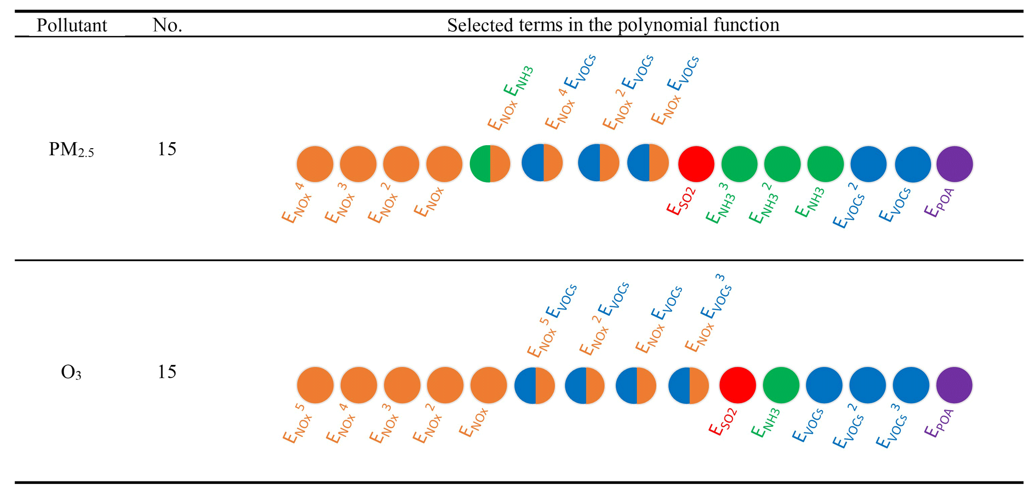
An example was shown in Supplement Fig. S1, which presents PM_2.5 responses to joint changes in NO_x and NH₃ emissions in July. The PM_2.5 response calculated using Eq. (4) (with all interaction terms) was consistent with that estimated using the regression-based RSM. The PM_2.5 response calculated using Eq. (5) (with no interaction terms) exhibited a noticeable discrepancy compared with those calculated using Eq. (4) and estimated using the regression-based RSM. With one selected interaction term, the PM_2.5 response exhibited a substantial improvement compared with that calculated using Eq. (4), thereby indicating interactions between NO_x and NH₃ emissions for PM_2.5. The results of term selections for both O₃ and PM_2.5 are summarized in Fig. 4. The interaction terms of NO_x and VOCs are included for both pollutants. SO₂ and POA did not interact with other species.

2.2.3 Sampling optimization

Training samples were generated to fit the polynomial function for each pollutant. To minimize the number of CTM simulations (one simulation scenario represents one training sample), the number of training samples needed to be as small as possible, but greater than the number of terms (i.e., unknown coefficients) in the polynomial function. Our previous study (Xing et al., 2011) suggested that samples generated through uniform methods, such as Latin hypercube sampling (LHS) and a Hammersley quasi-random sequence sample (HSS), could provide even distributions for individual sources. However, additional marginal processing is recommended for its ability to improve the performance of prediction at margins.

Sensitivity analysis of the number and distributions of training samples was conducted in this study. Groups of 20, 30, 40 or 50 training samples were sampled using uniformly distributed HSS. Additional marginal processing was conducted using a power function (n=2) from uniformly distributed HSS on the samples, expressed as follows:

$$\begin{array}{}\text{(6)}& {\displaystyle }\mathrm{\text{TX}}=\left\{\begin{array}{ll}{\left({\displaystyle \frac{X-a}{b-a}}\right)}^{\mathrm{2}}\times \mathrm{2}\times \left(b-a\right)+a,& X\le a+{\displaystyle \frac{b-a}{\mathrm{2}}}\\ \left[\mathrm{1}-{\left({\displaystyle \frac{b-X}{b-a}}\right)}^{\mathrm{2}}\times \mathrm{2}\right]\times \left(b-a\right)+a,& X>a+{\displaystyle \frac{b-a}{\mathrm{2}}}\end{array}\right.,\end{array}$$

where X is sampled from a uniformly distributed HSS in section [a, b] (in this study we selected [0, 1.2], which denotes that emission changes were from all controlled to a 20 % increase) and TX represents the samples after the marginal processing.

Table 2Out-of-sample dataset for validation.

Download Print Version | Download XLSX

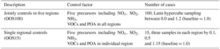
The training samples were predicted using the regression-based RSM and subsequently used to fit the polynomial function for all pollutants. We selected two datasets as out of sample to validate the fitting polynomial function, i.e., jointly controls in five regions (denoted as “OOS100”) and single regional controls (denoted as “OOS15”) (see Table 2). The control matrixes of these two datasets are provided in the Supplement (Table S1). The method of leave-one-out cross validation (LOOCV) was used to examine whether the statistical polynomial regression was overfitting. The definition of LOOCV is to use a single sample from the original datasets as the validation data, and the remaining sample as the training data to build pf-RSM.

The predictive performance of the pf-RSM was evaluated using five statistical indices, namely the mean normalized error (MeanNE), maximal normalized error (MaxNE), mean fractional error (MeanFE), maximal fractional error (MaxFE) and correlation coefficient (R), each calculated as follows:

$$\begin{array}{}\text{(7)}& {\displaystyle }& {\displaystyle }\text{MeanNE}={\displaystyle \frac{\mathrm{1}}{N}}{\sum }_{i=\mathrm{1}}^N{\displaystyle \frac{\left|M_i-O_i\right|}{O_i}}\text{(8)}& {\displaystyle }& {\displaystyle }\text{MaxNE}=max\left({\displaystyle \frac{\left|M_i-O_i\right|}{O_i}}\right)\text{(9)}& {\displaystyle }& {\displaystyle }\text{MeanFE}={\displaystyle \frac{\mathrm{1}}{N}}{\sum }_{i=\mathrm{1}}^N{\displaystyle \frac{\left|M_i-O_i\right|}{M_i+O_i}}\times \mathrm{2}\text{(10)}& {\displaystyle }& {\displaystyle }\text{MaxFE}=max\left({\displaystyle \frac{\left|M_i-O_i\right|}{M_i+O_i}}\times \mathrm{2}\right)\text{(11)}& {\displaystyle }& {\displaystyle }R=\sqrt{{\displaystyle \frac{\left[{\sum }_{i=\mathrm{1}}^N\left(M_i-\stackrel{\mathrm{‾}}{M}\right)\left(O_i-\stackrel{\mathrm{‾}}{O}\right)\right]}{{\sum }_{i=\mathrm{1}}^N{\left(M_i-\stackrel{\mathrm{‾}}{M}\right)}^{\mathrm{2}}{\sum }_{i=\mathrm{1}}^N{\left(O_i-\stackrel{\mathrm{‾}}{O}\right)}^{\mathrm{2}}}}},\end{array}$$

where M_i and O_i are the pf-RSM-predicted and CMAQ-simulated value of the ith data in the series, which can be a series of days, grid cells or control cases, and $\stackrel{\mathrm{‾}}{M}$ and $\stackrel{\mathrm{‾}}{O}$ are the average pf-RSM-predicted and CMAQ-simulated value over the series.

2.3 Indicators for representing nonlinearity in responses to precursor emissions

In our previous RSM studies, indicators representing the nonlinearity of O₃ and PM_2.5 responses to precursor emissions have been defined as the peak ratio (PR) for O₃ (Xing et al., 2011) and flex ratio (FR) for PM_2.5 (Wang et al., 2011), respectively.

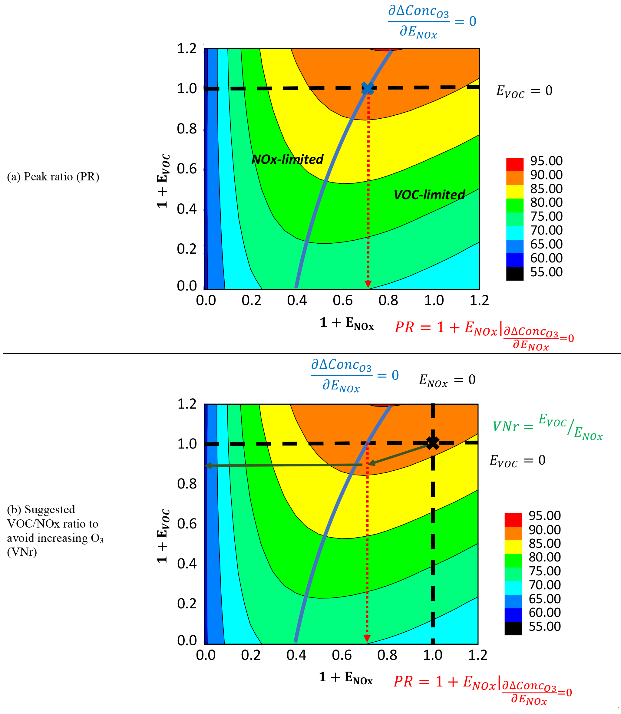
Figure 5Definition of peak ratio (PR) and suggested VOC ∕ NO_x ratio basing on the 2-D isopleths of O₃ sensitivity to NO_x and VOC emission changes (an example in Beijing in July).

Download

For O₃, the PR is the NO_x emissions that produce maximum O₃ concentrations under baseline VOC emissions (see in Fig. 5a). A PR lower than 1 (i.e., baseline) indicates that the baseline condition is VOC limited; in all other cases, the baseline condition is NO_x limited.

The previous calculations for the PR were performed through a looping procedure in the RSM statistical system, which is not straightforward. One advantage of the pf-RSM is that the PR can be directly calculated from the polynomial function as follows:

where $\frac{\partial \mathrm{\Delta }{\text{Conc}}_{{\mathrm{O}}_{\mathrm{3}}}}{\partial E_{{\mathrm{NO}}_x}}$ is the first derivation of the ${\text{Conc}}_{{\mathrm{O}}_{\mathrm{3}}}$ response to $E_{{\mathrm{NO}}_x}$.

In addition, we can further quantify how much simultaneous control of VOC is required to avoid increasing O₃ from the NO_x controls under VOC-limited conditions (see in Fig. 5b). The suggested VOC controls can be represented as the ratio of VOC to NO_x (denoted VNr), which can be calculated as follows:

where $\frac{\partial \mathrm{\Delta }{\text{Conc}}_{{\mathrm{O}}_{\mathrm{3}}}}{\partial E_{{\mathrm{NO}}_x}}$ is the first derivation of the ${\text{Conc}}_{{\mathrm{O}}_{\mathrm{3}}}$ response to $E_{{\mathrm{NO}}_x}$ when $E_{\text{VOC}}=X\times E_{{\mathrm{NO}}_x}$.

For PM_2.5, here we defined the FR as the NH₃ emission ratio at the flex nitrate (or PM_2.5) concentrations (i.e., when the second derivation of the function of concentration sensitivities to NH₃ emissions is zero) under baseline NO_x emissions (see in Fig. 6a). A FR greater than 1 indicates that the baseline condition is NH₃ poor (i.e., large sensitivity of PM_2.5 to NH₃); in all other cases, the baseline condition is NH₃ rich (small sensitivity of PM_2.5 to NH₃). The values of FR also suggest the transition point between two schemes.

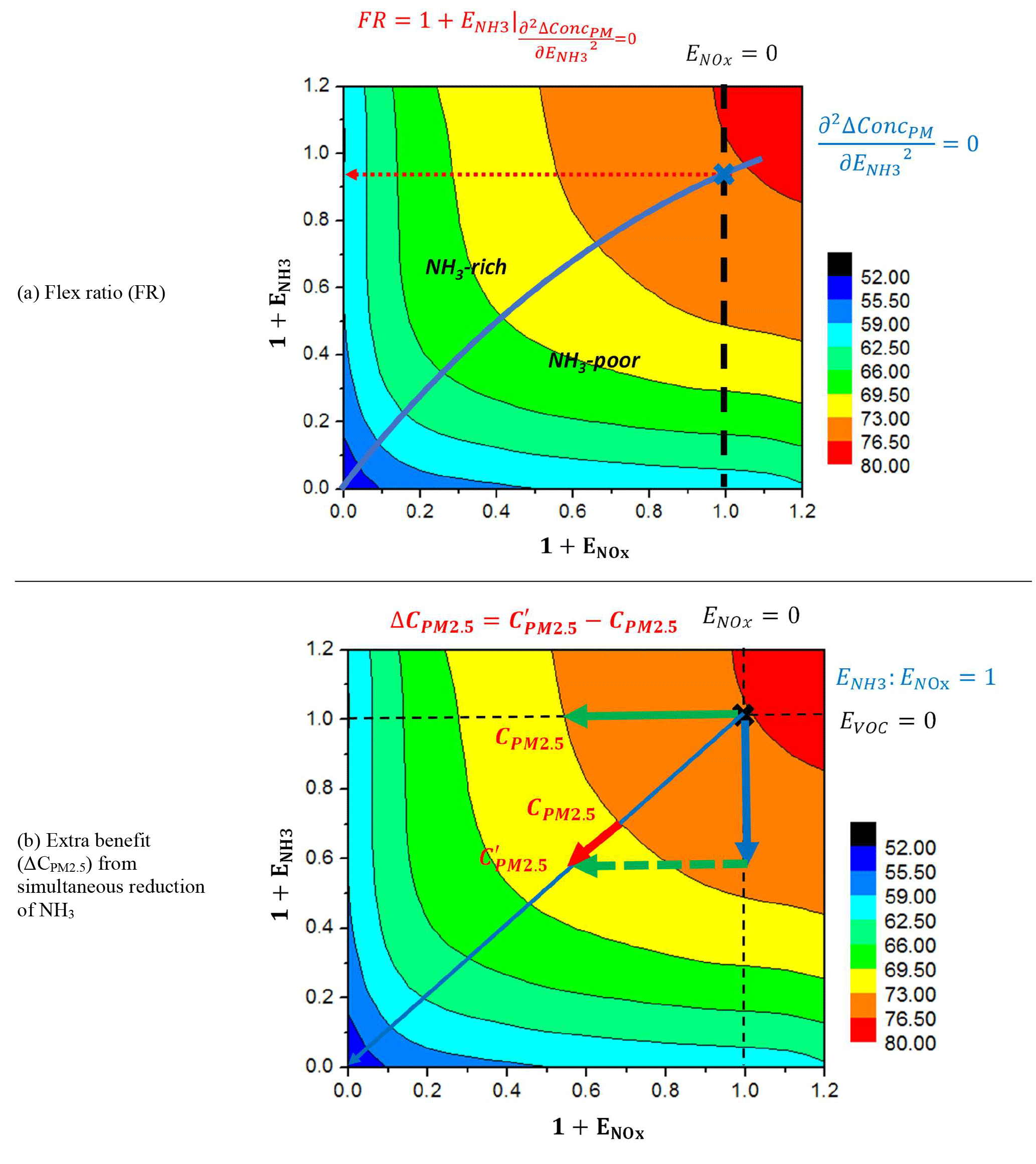
Figure 6Definition of flex ratio (FR) and extra benefit from simultaneous reduction of NH₃ basing on the 2-D isopleths of PM_2.5 sensitivity to NO_x and NH₃ emission changes (an example in Beijing in July).

Download

Similarly, the FR can be directly calculated from the polynomial function as follows:

where $\frac{{\partial }^{\mathrm{2}}\mathrm{\Delta }{\text{Conc}}_{\text{PM}}}{\partial {E_{{\mathrm{NH}}_{\mathrm{3}}}}^{\mathrm{2}}}$ is the second derivation of the Conc_PM response to $E_{{\mathrm{NH}}_{\mathrm{3}}}$.

Further, we can quantify the extra benefit in PM_2.5 reductions (denoted as ΔC) from simultaneous reduction of NH₃ along with the control of NO_x (see in Fig. 6b), which can be calculated as follows:

where $\frac{\partial \mathrm{\Delta }{\text{Conc}}_{{\text{PM}}_{\mathrm{2.5}}}}{\partial E_{{\mathrm{NO}}_x}}{\mathrm{|}}_{E_{{\mathrm{NH}}_{\mathrm{3}}}=E_{{\mathrm{NO}}_x}}$ is the first derivation of the ${\text{Conc}}_{{\text{PM}}_{\mathrm{2.5}}}$ response to $E_{{\mathrm{NO}}_x}$ when $E_{{\mathrm{NH}}_{\mathrm{3}}}=E_{{\mathrm{NO}}_x}$; $\frac{\partial \mathrm{\Delta }{\text{Conc}}_{{\text{PM}}_{\mathrm{2.5}}}}{\partial E_{{\mathrm{NO}}_x}}{\mathrm{|}}_{E_{{\mathrm{NH}}_{\mathrm{3}}}=\mathrm{0}}$ is the first derivation of the ${\text{Conc}}_{{\text{PM}}_{\mathrm{2.5}}}$ response to $E_{{\mathrm{NO}}_x}$ when $E_{{\mathrm{NH}}_{\mathrm{3}}}=\mathrm{0}$.

The PR and FR are the results of $\mathrm{1}+E_{{\mathrm{NO}}_x}$ and $\mathrm{1}+E_{{\mathrm{NH}}_{\mathrm{3}}}$, respectively, corresponding to the extreme value point and inflexion point of ${\text{Conc}}_{{\mathrm{O}}_{\mathrm{3}}}$ and Conc_PM, respectively, in section [a, b] (i.e., [0, 1.2] in this study). The ratios of VOC to NO_x and ΔC were estimated for the five regions in BTH.

3.1 Sensitivity analysis on training sample number and distribution

Table 3 summarizes the performance of the pf-RSM with different training samples for predicting PM_2.5 and O₃. For out-of-sample validation (i.e., OOS100 and OOS15), good agreement was observed in all cases. Even with 20 training samples (only five more than the number of terms in the polynomial function), the MeanNE and MeanFE were lower than 3.1 and 1.5 %, respectively, and the MaxNE and MaxFE were lower than 15.1 and 7.0 %, respectively. The R values were greater than 0.8. The performance improved with an increase in training sample number. When 50 training samples were selected, the MeanNE and MeanFE were lower than 1.7 and 0.8 %, respectively, and the MaxNE and MaxFE were lower than 8.7 and 4.2 %, respectively. The R values were greater than 0.94.

Additional marginal processing improved the performance of PM_2.5 and O₃ prediction by reducing the maximal errors rather than the mean errors. In all cases, the MaxNE and MaxFE in O₃ decreased from 12.4 and 5.8 % to 5.5 and 2.7 %, respectively. The MaxNE and MaxFE in PM_2.5 slightly decreased from 15.1 and 6.98 % to 15.0 and 6.97 %, respectively.

To meet the criteria of MeanNE within 2 % and MaxNE within 10 % (i.e., uncertainty of pf-RSM), which is comparable to the performance of previous regression-based RSMs, the use of 40 training samples with marginal processing (to improve boundary conditions) is recommended.

Similar results are found in the cross validation (i.e., LOOCV), as the performance in pf-RSM gets better along with the increase in sample numbers. Basically, the statistics of cross validation are in the same order as shown in out-of-sample validations (OOS100 and OOS15), except for the case of 20 training samples with marginal processing (worse performance due to underfitting problem). One interesting finding is that the pf-RSM with marginal processing exhibits worse performance than that with an even sampling method in cross validation. That is because the samples with marginal processing are located closer to margin areas where it is more difficult to predict (Xing et al., 2011). This also implies that the samples with marginal processing have better representation of the variability. Nevertheless, the results of validations suggest the pf-RSM with the current number of samples is not overfitted, and the number of training samples selected in fitting the system is recommended to be 40 training samples with marginal processing.

One kind of visual comparison, i.e., isopleth validation of the pf-RSM with different training samples was conducted, and its details are shown in the Supplement (Fig. S2–S9). The performance of the pf-RSM with less than 40 training samples exhibited a noticeable discrepancy (i.e., spatial pattern of the response under the controls) compared with that of the regression-based RSM. Such discrepancy is caused by the underfitting issue, implying that the number of training samples is not large enough to capture the nonlinearity in the model system. The issue can be addressed by adding more training samples to fit the model. The 40 training samples presented good agreement with the predictions of the regression-based RSM. An improved sampling method is also important for reducing the biases. We can see that additional marginal processing also improved the performance of the pf-RSM.

3.2 Application of the polynomial function at different locations and times

First, we applied the pf-RSM in each grid cell in the simulated domain. The base case and 40 controlled scenarios simulated by the CMAQ model (41 training samples in total) were used to fit the function of each grid cell. Two out-of-sample CMAQ cases (i.e., Case 1: moderate control with $E_{{\mathrm{NO}}_x}$, $E_{{\mathrm{SO}}_{\mathrm{2}}}$, $E_{{\mathrm{NH}}_{\mathrm{3}}}$, E_VOCs and E_POA $=-$49, −45, −20, −64 and −20 % respectively; Case 2: strict control with $E_{{\mathrm{NO}}_x}$, $E_{{\mathrm{SO}}_{\mathrm{2}}}$, $E_{{\mathrm{NH}}_{\mathrm{3}}}$, E_VOCs and E_POA $=-$76, −79, −81, −83 and −73 %, respectively) were used to validate the performance of the pf-RSM. These two scenarios are selected from the OOS100 to represent two kinds of emission levels, moderate and strict, for the purpose of analyzing the pf-RSM performance under different locations and times. Please note that the validation results might slightly change if we change the scenarios; however, the performance should be similar to the two we presented here (see comparison with the other nine cases shown in Fig. S10).

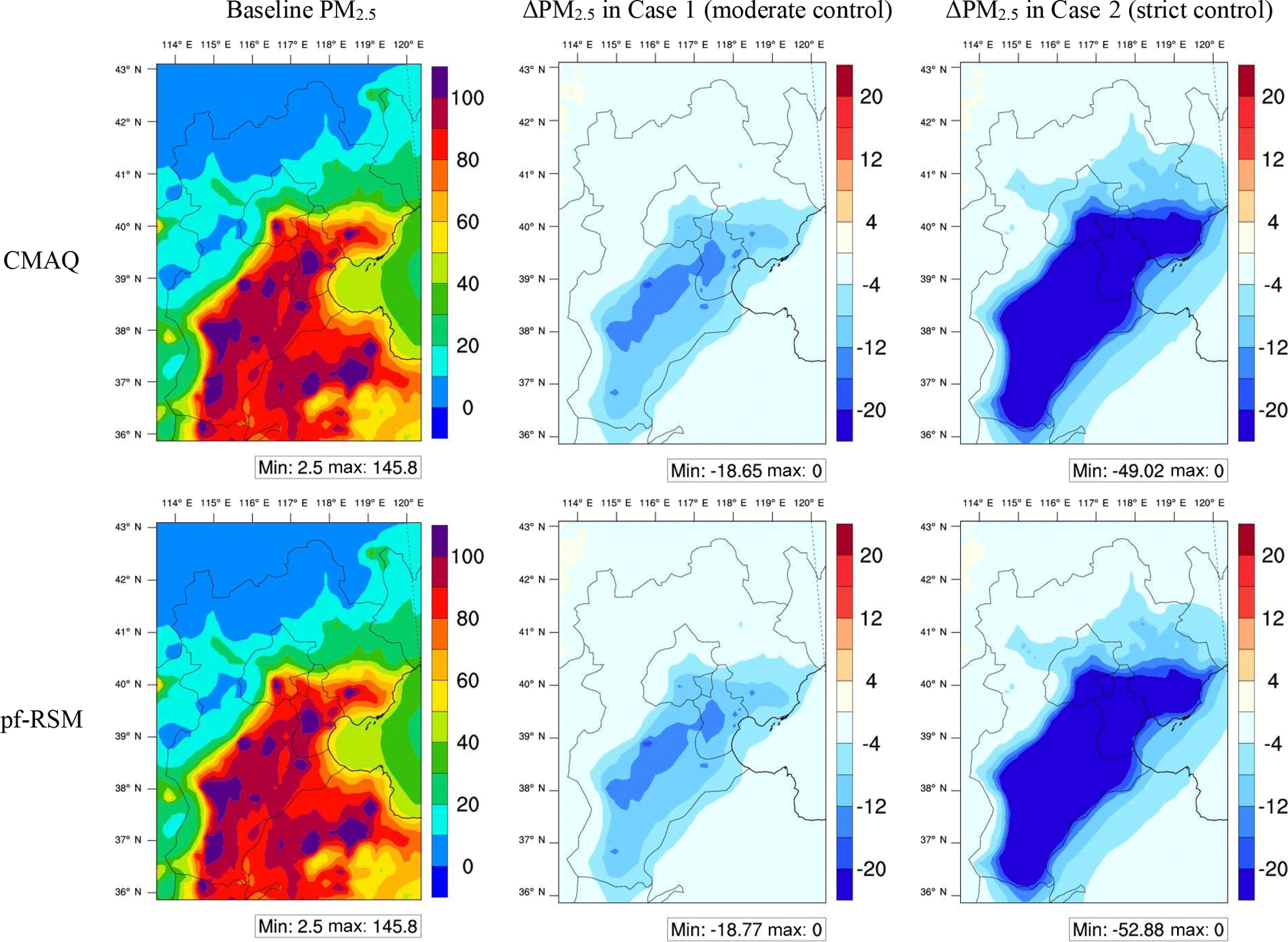
Figure 7Spatial distribution of CMAQ-simulated and pf-RSM-predicted PM_2.5 in the baseline and PM_2.5 responses in two control scenarios (monthly averages in January 2014, unit: µg m⁻³, $E_{{\mathrm{NO}}_x}$, $E_{{\mathrm{SO}}_{\mathrm{2}}}$, $E_{{\mathrm{NH}}_{\mathrm{3}}}$, E_VOCs and E_POA in Case 1 and Case 2 are −49, −45, −20, −64, and −20 and −76, −79, −81, −83, and −73 %, respectively).

Download

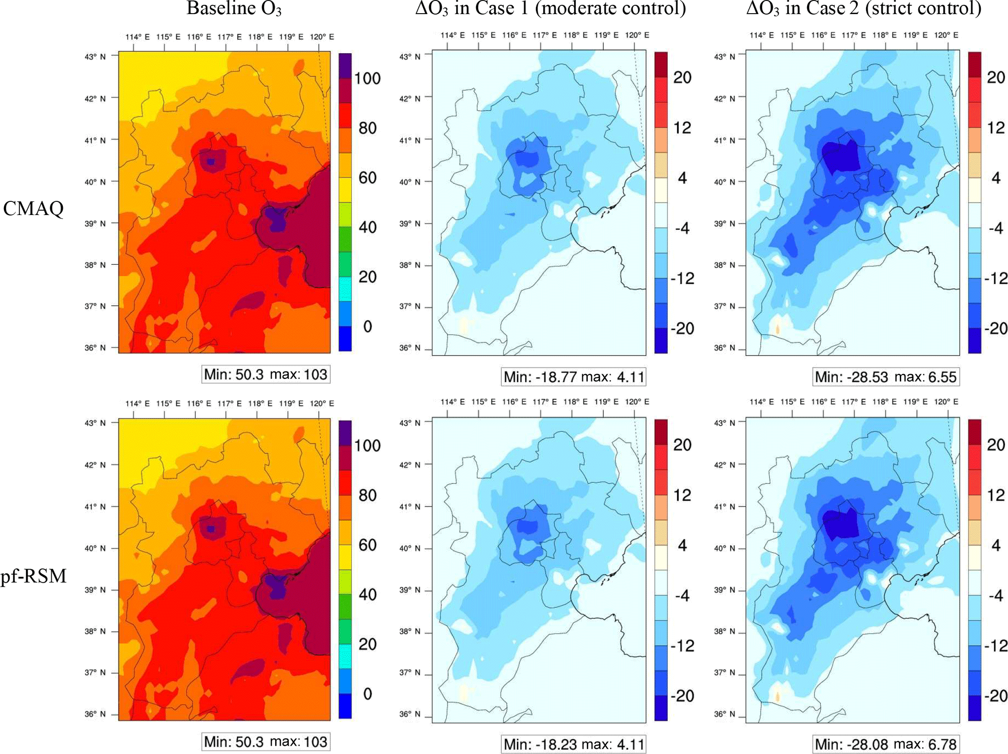
Figure 8Spatial distribution of CMAQ-simulated and pf-RSM-predicted O₃ in baseline and O₃ responses in two control scenarios (monthly averages of daily 1 h maxima O₃ in July 2014, unit: ppb, $E_{{\mathrm{NO}}_x}$, $E_{{\mathrm{SO}}_{\mathrm{2}}}$, $E_{{\mathrm{NH}}_{\mathrm{3}}}$, E_VOCs and E_POA in Case 1 and Case 2 are −49, −45, −20, −64, and −20 and −76, −79, −81, −83, and −73 %, respectively).

Download

Figures 7 and 8 present the spatial distribution of CMAQ-simulated and pf-RSM-predicted PM_2.5 and O₃ in the baseline and their responses in two control scenarios. PM_2.5 predictions by the pf-RSM exhibited the same values in the baseline scenario as those simulated by the CMAQ model because the ΔConc is 0 with no perturbations in emissions; Eq. (1). With the reduction of emissions in the two control cases, the PM_2.5 and O₃ concentrations were reduced substantially in the CMAQ and pf-RSM predictions. The pf-RSM and CMAQ made very similar predictions for both cases, with normalized errors all within 5.6 % for PM_2.5 and 2.0 % for O₃ across the domain.

The performance of PM_2.5 and O₃ prediction in the pf-RSM across grid cells was summarized in Table S2. Larger errors were shown in Case 2 than in Case 1 because of relatively poor performance at the margin areas, where emissions were greatly controlled (Xing et al., 2011). Under moderate control condition (i.e., Case 1), smaller errors were observed in polluted regions for PM_2.5 and O₃ because of larger denominators (i.e., a high concentration). However, under strict control conditions (i.e., Case 2), larger errors were evident in more polluted regions, particularly for PM_2.5, indicating that the biases due to marginal effects were more prevalent in polluted regions.

Second, we applied the pf-RSM to each day in two simulated months (i.e., January and July, 2014). The same 41 training samples and two additional CMAQ cases were used to fit and validate the pf-RSM on each day.

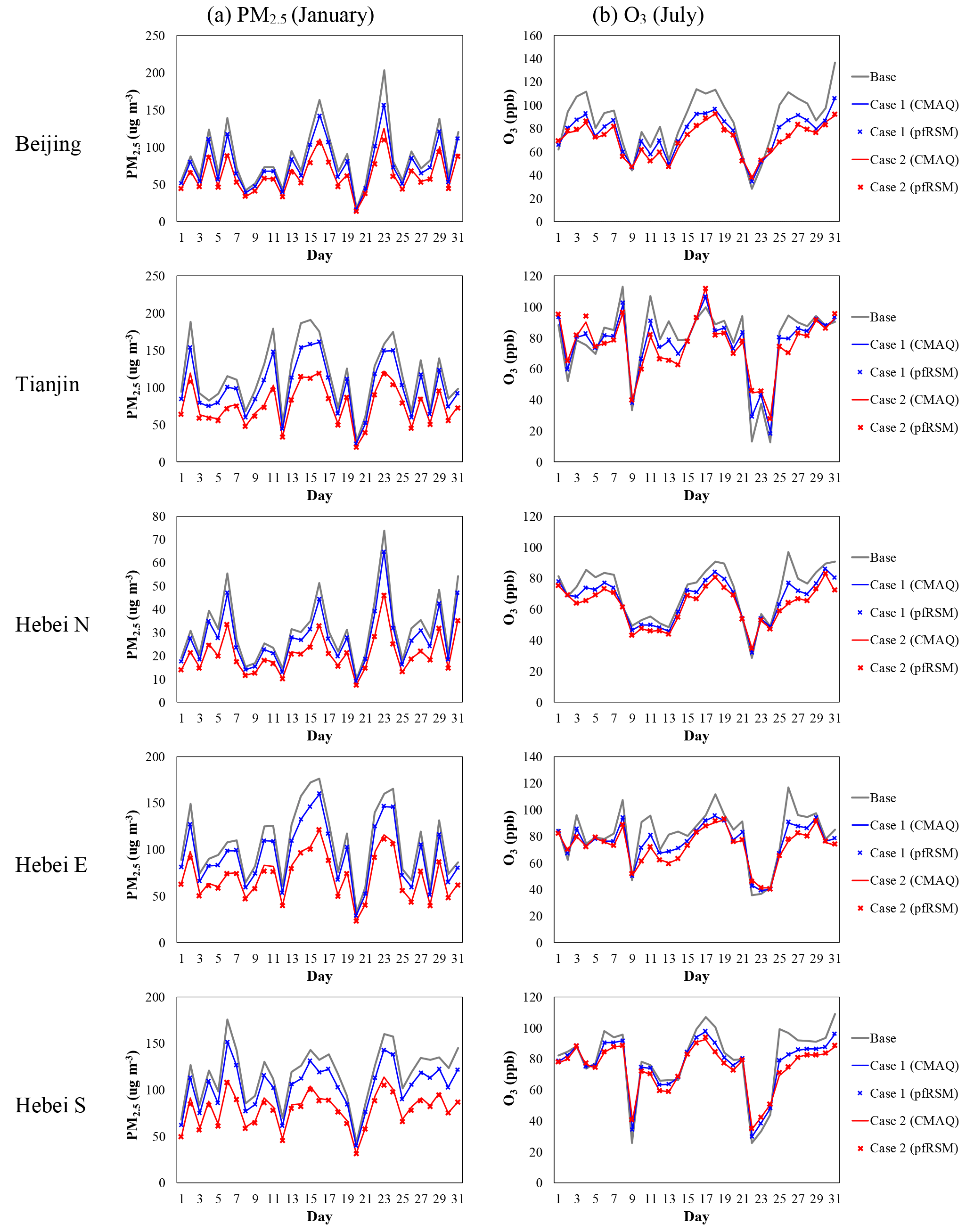
Figure 9Daily series of CMAQ-simulated and pf-RSM-predicted daily averaged PM_2.5 in January and daily 1 h maxima O₃ in July 2014 in the baseline and two control scenarios ($E_{{\mathrm{NO}}_x}$, $E_{{\mathrm{SO}}_{\mathrm{2}}}$, $E_{{\mathrm{NH}}_{\mathrm{3}}}$, E_VOCs and E_POA in Case 1 and Case 2 are −49, −45, −20, −64, and −20 and −76, −79, −81, −83, and −73 %, respectively).

Download

The daily series of the CMAQ-simulated and pf-RSM-predicted 24 h averaged PM_2.5 and 1 h maxima O₃ in the baseline and two control scenarios are shown in Fig. 9. The day-to-day variability in O₃ depends on the budget of O₃ source and sink influenced by meteorological variables including actinic flux, temperature, humidity and precipitation, etc. Generally, the pf-RSM-predicted daily PM_2.5 and O₃ concentrations matched with CMAQ model simulations fairly well, with normalized errors within 12.7 and 6.5 % for PM_2.5 and O₃, respectively. Substantial reductions in PM_2.5 were observed in Case 2, in which strict controls were applied. Noticeable biases were observed on 23 January when PM_2.5 levels were high in Beijing and HebeiS. The meteorological conditions will also play an important role in the effectiveness of emission controls. Reductions in O₃ were noticeable in both control cases, particularly on days when O₃ levels were high. However, increases in O₃ were observed on 21–23 July (precipitation event occurred across North China Plain), after the controls were applied and when O₃ levels were low. This can be explained by the O₃ chemistry scheme being at a strong VOC-limited conditions on days with low O₃ levels, resulting in enhanced O₃ from NO_x controls (Xing et al., 2011). Thus, the emission controls usually become less effective under unfavorable meteorological conditions for O₃ production. The pf-RSM also reproduced increases in O₃ on those days.

Table 3Performance of PM_2.5 and O₃ prediction using pf-RSM with different training samples.

¹PM_2.5 and O₃ responses are calculated based on monthly averaged concentrations for averages of urban sites. ² LOOCV: “leave-one-out cross validation” in which a single sample from the original datasets is used as the validation data, and the remaining samples as the training data to build pf-RSM.

Download Print Version | Download XLSX

The performance of PM_2.5 and O₃ prediction in the pf-RSM throughout the simulation period was summarized in Table S3. The MeanNEs for PM_2.5 and O₃ were within 3.7 and 1.3 %, respectively. Larger errors were evident in Case 2 than in Case 1 because of poor performance at margin areas, where emissions are greatly controlled (Xing et al., 2011). These biases in Case 2 became larger on more polluted days, particularly for PM_2.5, suggesting that marginal biases were more evident during polluted period.

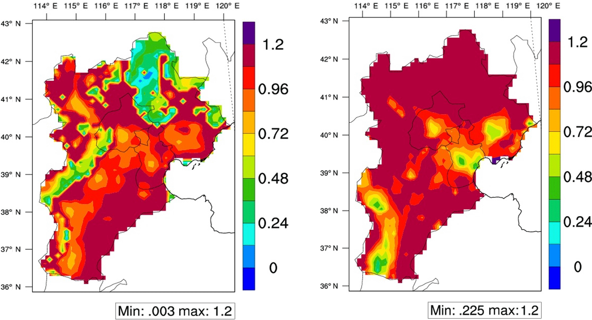
Figure 10Spatial distribution of the indicators for PM_2.5 (flex ratio, FR) in January and O₃ chemistry (peak ratio, PR) in July 2014.

Download

3.3 Quantification of nonlinearities in control effectiveness for reducing PM_2.5 and O₃

The nonlinearity in the pollution response to emissions leads to an either enhanced or reduced effectiveness of emission controls. In previous studies, the concept of NH₃-limited/NH₃-poor and NO_x-/VOC-limited conditions was used widely to demonstrate the influence of NH₃ and VOC on effectiveness of NO_x controls for reducing PM_2.5 and O₃, respectively. However, some key questions were not well addressed, such as what percentage of NO_x or NH₃ is overabundant and what percentage of VOC needs to be reduced simultaneously to avoid increased O₃. In this study, the newly developed pf-RSM explicitly represents the response, and the enhanced effectiveness can be easily quantified. The indicators defined in Sect. 2.3 can be used to quantify the nonlinear effectiveness of emission control for reducing PM_2.5 and O₃. The FR values across grid cells were calculated using Eq. (14) for PM_2.5 chemistry in January (Fig. 10a). Most of the study regions exhibited FR values lower than 1, suggesting strong NH₃-rich conditions. These results are consistent with those of previous studies (Liu et al., 2010; Wang et al., 2011). Larger FR values (slightly lower than 1.0) were shown in the central and southern regions (i.e., Beijing, Tianjin and HebeiS) than in other regions, suggesting that the PM_2.5 concentrations were sensitive to both NO_x and NH₃ controls, possibly because of the high SO₂ and NO_x emissions in Beijing, Tianjin and HebeiS (Zhao et al., 2016), which led to the high consumption of NH₃ neutralized with H₂SO₄ and HNO₃, as well as high PM_2.5 concentrations (Fig. 5).

Table 4 summarized the indicators at urban areas of prefecture-level cities in the five target regions. In both January and July, most of the urban areas (except strong NH₃-poor conditions in HebeiN in July) present NH₃-rich condition with a FR from 0.75 to 0.95 (Table 4), implying NH₃ is sufficiently abundant to neutralize extra nitric acid produced by an additional 5–35 % (i.e., =1 ∕ FR-1) of NO_x emissions. The result is consistent with our previous study (Wang et al., 2011), which reported that NH₃ is sufficiently abundant to neutralize extra nitric acid produced by an additional 25 % of NO_x emissions in the North China Plain based on a traditional regression-based RSM study. The extra benefit in PM_2.5 reductions from simultaneous reduction of NH₃ along with the control of NO_x was estimated to be 0.04–0.15 µg m⁻³ PM_2.5 per 1 % reduction of NH₃. A larger benefit in PM_2.5 reductions by simultaneous reduction of NH₃ was found in July when the NH₃-rich conditions were not as strong as in January.

Table 4Estimation of indicators that represent the nonlinear control effectiveness for reducing PM_2.5 and O₃ in the Beijing–Tianjin–Hebei region.

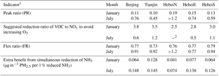
¹ Indicators are calculated based on monthly averaged concentrations at urban areas of prefecture-level cities in the five target regions. ² Since the PR is larger than 1.2 in HebeiN, the NO_x control will always lead to a reduction in O₃.

Download Print Version | Download XLSX

The PR values for O₃ chemistry in July were calculated using Eq. (12), as shown in Fig. 10b. Different PR values were observed in urban and downwind areas. That is consistent with the findings of previous studies (Xing et al., 2011), which used a traditional regression-based RSM and found that the PR changes from 0.8 to 1.2 as the distance from the city center increases. Smaller PRs (0.4–0.8, see Table 4) were evident in urban areas (i.e., megacities such as Beijing, Tianjin, Shijiazhuang and Tangshan), where NO_x emissions are saturated, resulting in strong VOC-limited conditions. Our results are consistent with the observational studies that use an indicator to identify the O₃ chemistry. For example, Liu et al. (2016) studied the ratios of HCHO over NO₂ from the satellite retrievals and found that local ozone production in urban Beijing is VOC limited when there are no substantial changes in NO_x emission in 2015. Chou et al. (2009) found that the Beijing urban area was a VOC-limited region based on the observation of NO, NO_x and NO_y at the Peking University site from 15 August to 11 September in 2006. Jin and Holloway (2015) calculated the ratio of HCHO to NO₂ from the OMI instrument aboard the Aura satellite and found the O₃ production is more likely to be VOC limited over urban areas and NO_x limited over rural and remote areas in China from 2005 to 2013.

The PR values calculated in this study also indicate that the control of NO_x (with less than 20–60 % reduction, = 1 − PR) could result in an increase in O₃; however, O₃ would decrease with substantial control of NO_x (with greater than 20–60 % reduction). To avoid increasing O₃ during the transition from VOC-limited to NO_x-limited conditions, a simultaneous VOC reduction by 0.5–1.2 times the rate of NO_x reduction is recommended. Stronger VOC-limited conditions are found in January, while O₃ concentration is considerably lower than in July. However, the strong VOC-limited conditions in January will also lead to a considerable disbenefit of NO_x reduction for PM_2.5 controls (see the isopleth plot of PM_2.5 response to NO_x and NH₃ emission changes in Fig. S6, also found in Zhao et al., 2017) because the enhanced atmospheric oxidation ability from reducing NO_x under VOC-limited conditions will facilitate the formation of secondary aerosols. Therefore simultaneous VOC reduction can help avoid such increase of PM_2.5 associated with NO_x controls under strong VOC-limited condition in January. Notably, the O₃ discussed in this paper refers to the monthly averages of daily 1 h maximum values. The PR values varied considerably between the clean and polluted days, suggesting mostly NO_x-limited conditions during polluted periods, which are usually subject to a more severe O₃ burden (Xing et al., 2011). Nevertheless, the control of NO_x emissions is critical for reducing regional O₃ and PM_2.5; however, it is recommended to simultaneously reduce VOC and NH₃ emissions along with NO_x reduction to avoid the risk of increasing O₃ and gain extra benefit in PM_2.5 reduction.