the Creative Commons Attribution 4.0 License.
the Creative Commons Attribution 4.0 License.
 | 01 Jun 2018
Impact of high-resolution a priori profiles on satellite-based formaldehyde retrievals
Vijay Natraj
Seoyoung Lee
Hyeong-Ahn Kwon
Rokjin Park
Joost de Gouw
Gregory Frost
Jhoon Kim
Jochen Stutz
Michael Trainer
Catalina Tsai
Carsten Warneke
Formaldehyde (HCHO) is either directly emitted from sources or produced during the oxidation of volatile organic compounds (VOCs) in the troposphere. It is possible to infer atmospheric HCHO concentrations using space-based observations, which may be useful for studying emissions and tropospheric chemistry at urban to global scales depending on the quality of the retrievals. In the near future, an unprecedented volume of satellite-based HCHO measurement data will be available from both geostationary and polar-orbiting platforms. Therefore, it is essential to develop retrieval methods appropriate for the next-generation satellites that measure at higher spatial and temporal resolution than the current ones. In this study, we examine the importance of fine spatial and temporal resolution a priori profile information on the retrieval by conducting approximately 45 000 radiative transfer (RT) model calculations in the Los Angeles Basin (LA Basin) megacity. Our analyses suggest that an air mass factor (AMF, a factor converting observed slant columns to vertical columns) based on fine spatial and temporal resolution a priori profiles can better capture the spatial distributions of the enhanced HCHO plumes in an urban area than the nearly constant AMFs used for current operational products by increasing the columns by ∼ 50 % in the domain average and up to 100 % at a finer scale. For this urban area, the AMF values are inversely proportional to the magnitude of the HCHO mixing ratios in the boundary layer. Using our optimized model HCHO results in the Los Angeles Basin that mimic the HCHO retrievals from future geostationary satellites, we illustrate the effectiveness of HCHO data from geostationary measurements for understanding and predicting tropospheric ozone and its precursors.
- Article
(5070 KB) -
Supplement
(3063 KB) - BibTeX
- EndNote


Formaldehyde (HCHO) is directly released to the atmosphere from sources that include motor vehicles, industrial activities, prescribed burnings, and wildfires. HCHO is one of the hazardous air pollutants (HAPs) – that are harmful to human health – defined by the US Environmental Protection Agency (see US EPA, 2015a, for more information). More importantly, HCHO is chemically produced during volatile organic compound (VOC) oxidation processes (Wolfe et al., 2016) and is therefore correlated with major chemical species formed during photochemical smog episodes (e.g., ozone, O3). Because of the close relationship between HCHO and its VOC precursors, the ratio of satellite HCHO columns to nitrogen dioxide (NO2) columns has been suggested as an indicator of photochemical regimes; i.e., the ratio determines VOC-limited (or sensitive) or NOx-limited (or sensitive) regimes of O3 formation in a certain location and season (Martin et al., 2004a; Jin et al., 2017). In the presence of NOx, HCHO can be a major source of hydroxyl radical (OH), the most important chemical species in the troposphere initiating photochemical chain reactions. The chemical lifetime of HCHO with respect to loss by OH reaction and photolysis is several hours (Warneke et al., 2011). HCHO is highly soluble and may contribute to aqueous chemical processes in clouds and precipitation in the atmosphere and in bodies of water at the Earth's surface (Barth et al., 2007; Luecken et al., 2012).
Due to its importance to tropospheric chemistry, atmospheric chemists and the environmental remote sensing community have sought to produce high-quality tropospheric HCHO retrievals. Because of its weak absorption in the ultraviolet (UV) spectral region, HCHO is regarded as one of the most difficult species to retrieve from satellite-based radiance observations in the UV–visible (UV-VIS) spectral region (e.g., GOME/GOME-2, SCIAMACHY, OMI, and OMPS; see Martin et al., 2004b; Zhu et al., 2016, for references). In addition, large uncertainties in satellite trace gas retrievals based on UV-VIS spectral measurements arise from the calculation of the air mass factor (AMF), which converts the slant column density of a trace gas to its vertical column values by considering the vertical sensitivity of the observations (AMF = slant column/vertical column, Palmer et al., 2001; Boersma et al., 2004; Lorente et al., 2017). Therefore, it is important to identify factors affecting the accuracy of HCHO retrievals and to find a method to reduce these uncertainties.
Palmer et al. (2001) expressed the AMF as a vertical integral of the product of scattering weight functions and normalized vertical profile shapes of trace gases that vary with atmospheric heights. The scattering weight function can be precalculated in a lookup table using radiative transfer (RT) model simulations, while the a priori profiles are generally derived from a three-dimensional chemical transport model. This formulation has been widely used to derive operational trace gas retrieval products (e.g., González Abad et al., 2015; De Smedt et al., 2018).
In this study, we examine the role of trace gas vertical profile shapes on HCHO retrievals in the Los Angeles (LA) Basin megacity. The HCHO retrievals from existing polar-orbiting satellites were investigated and utilized in previous studies (e.g., Palmer et al., 2001; Millet et al., 2008; Stavrakou et al., 2015; González Abad et al., 2015; Zhu et al., 2016); these studies focused on regions with large biogenic sources or showed large scale contrasts between land and ocean. Zhu et al. (2014) estimated the anthropogenic VOC emissions from large industrial complexes in Houston, Texas, by oversampling Ozone Monitoring Instrument (OMI) HCHO columns. In the near future, HCHO retrievals will be available from both geostationary (e.g., TEMPO, Fishman et al., 2012, and Zoogman et al., 2017; GEMS, Kim and the GEMS Team, 2012; Sentinel-4, Ingmann et al., 2012, and Veihelmann et al., 2015) and polar-orbiting (e.g., TROPOMI, Veefkind et al., 2012) platforms with much finer temporal and spatial resolutions, enabling satellite-based air quality studies at suburban to urban scales. HCHO retrievals at these scales may need a better strategy to deal with spatial and temporal variability in a priori vertical profiles of measured tracers than current methods that rely on profile shapes generated by coarse (horizontal grid resolutions of 1–3∘) global models. For example, Heckel et al. (2011) investigated the impacts of the spatial resolution of a priori profiles on NO2 retrievals in a coastal city (San Francisco, California), which highlighted the need for high-resolution a priori data to quantitatively probe tropospheric pollution in coastal regions and near localized sources such as power plants. Russell et al. (2011) also found non-negligible impacts of high spatial and temporal resolution terrain and profile inputs on the OMI NO2 retrievals. Kwon et al. (2017) emphasized the importance of using hourly varying HCHO AMF for geostationary satellite measurements in East Asia mainly due to temporal changes in aerosol chemical composition and vertical distributions.
In this study, we simulate fine-resolution (4 km × 4 km) vertical profiles for HCHO retrievals and investigate the spatiotemporal variability of the HCHO AMF based on these profiles. We also show the usefulness of detailed spatial and temporal information on HCHO plume structures at an urban scale for interpreting the effectiveness of ozone pollution controls.
2.1 Aircraft and ground-based measurements
2.1.1 NOAA WP-3 aircraft observations
During the California Nexus of Air Quality and Climate Change (CalNex) campaign, the NOAA WP-3 aircraft performed 20 research flights mainly over the Los Angeles Basin (LA Basin) and the Central Valley in California during May and June 2010 (see Ryerson et al., 2013, for more information). The main goals of CalNex were to quantify the emissions of greenhouse gases and ozone and aerosol precursors and to understand the chemical transformations and the transport of pollutants. The NOAA WP-3 aircraft was equipped with a large suite of gas phase and aerosol measurements. In this study, we use the HCHO measurement of a proton-transfer-reaction mass spectrometry (PTR-MS) instrument onboard the WP-3 aircraft (Warneke et al., 2011). Airborne HCHO measurements by PTR-MS are difficult due to a strong humidity dependency. The detection limit for HCHO with this instrument is between 100 pptv in the dry free troposphere and 300 pptv in the humid marine boundary layer. The PTR-MS HCHO measurements have been shown to agree with differential optical absorption spectroscopy (DOAS) observations (Stutz and Platt, 1997; Platt and Stutz, 2008) within the stated uncertainties. For comparison, the model results are first sampled at the times and locations of the observations. Then the PTR-MS measurement data onboard the P3 aircraft and the sampled model data are averaged at the model spatial resolution (horizontal and vertical) to allow one-to-one comparison of the observations and model results.
2.1.2 UCLA long-path DOAS data in Pasadena during CalNex
UCLA's long-path (LP)-DOAS instrument (Stutz and Platt, 1997; Platt and Stutz, 2008) is located on the California Institute of Technology (Caltech) campus on the roof of the Millikan Library at 35 m a.g.l. (above ground level). Four retro-reflectors are situated northeast of the main instrument in the mountains behind Altadena at 78, 121, 255, and 556 m a.g.l. The average distance between the LP-DOAS telescope and the reflectors is about 6 km. Spectral retrievals of HCHO mixing ratios were performed in the 324–346 nm wavelength range using a combination of a linear and nonlinear least squares fit, as described in Stutz and Platt (1996) and Alicke et al. (2002). Spectral absorption features of O3, NO2, HONO, O4, and HCHO were incorporated in the fitting procedure. The campaign-averaged statistical HCHO error in the DOAS measurements during CalNex was about 150 pptv (Warneke et al., 2011). In the present study, we use these ground-based DOAS data since vertical distribution information resulting from the four retroreflectors at different altitudes allows for comparison with the model results. The LP-DOAS data are averaged over the upper light path from 35 m a.g.l. (Millikan Library at Caltech) to 225 m a.g.l. (water tank in Altadena) and are averaged for 1 h prior to the comparison with the model results. The model values on the vertical levels corresponding to 35 to 225 m a.g.l. are averaged for the comparison with the LP-DOAS data. The model value from the 4 km × 4 km horizontal grid cell containing the Millikan Library at Caltech is selected for the comparison with the LP-DOAS observations.
2.1.3 The AQMD surface monitoring data
The hourly O3 data from the South Coast Air Quality Management District (AQMD) monitoring network (http://www.arb.ca.gov/aqmis2/aqdselect.php, last access: 28 May 2018) are utilized for the trend study. Details on standard procedures for maintaining and operating air monitoring stations and specific instrumentations are provided in the CARB air monitoring web manual (http://www.arb.ca.gov/airwebmanual/index.php, last access: 28 May 2018). The locations of the sites and the data are shown in the supporting information in Kim et al. (2016).
2.2 WRF-Chem model
We use version 3.4.1 of the Weather Research and Forecasting (WRF) model coupled with Chemistry (WRF-Chem, Grell et al., 2005). The model physical and chemical settings are the same as those used by Kim et al. (2016). The mother and the nested domains of the WRF-Chem model are the western US (12 km × 12 km horizontal resolution) and the state of California (4 km × 4 km horizontal resolution), respectively. The model has 60 vertical levels with ∼ 50 m thickness between vertical levels up to 4 km a.g.l., with coarser vertical resolution at higher levels. The first model level where mixing ratios of chemical species are calculated is ∼ 25 m. The simulation period is 26 April–17 July 2010. Meteorological initial and boundary conditions are based on NCEP Global Forecast System data. The MOZART (Model for OZone And Related chemical Tracers, http://www.acom.ucar.edu/wrf-chem/mozart.shtml, last access: 28 May 2018) (Emmons et al., 2010) global model results are used as initial and boundary conditions for the mother domain of WRF-Chem. Biogenic emissions are based on the Biogenic Emissions Inventory System (BEIS) version 3.13, with additional emissions from urban vegetation (Scott and Benjamin, 2003). The Noah land surface model, Yonsei University planetary boundary layer model, Lin microphysics scheme, and Grell–Devenyi ensemble cumulus parameterization (only for the mother domain) are adopted (see references in Kim et al., 2009). The chemical mechanism is based on the Regional Atmospheric Chemistry Mechanism (RACM) (Stockwell et al., 1997) with ∼ 30 reaction rate coefficients updated (Kim et al., 2009).
We adopt the NOx and CO emission estimates from Kim et al. (2016) that utilized the fuel-based approaches of McDonald et al. (2012, 2013, 2014). For VOC emissions, we used the emission estimates from the top-down approach employing ground-based observations in Pasadena, as described by Borbon et al. (2013), along with the US EPA NEI05 (US EPA, 2008; Kim et al., 2011, 2016) and NEI11 (US EPA, 2015b; Ahmadov et al., 2015) inventories. The HCHO model results using the top-down VOC emissions approach are the focus of this paper.
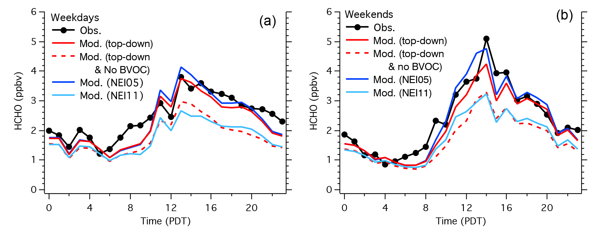
Figure 1Diurnal variations of ground-based observations (black filled circles with solid lines) of HCHO and the corresponding model simulations (lines without symbols) in Pasadena (34.1370∘ N, 118.1254∘ W) averaged for weekdays (a) and weekends (b) during May–June 2010. All model simulations utilized the fuel-based NOx and CO emissions in Kim et al. (2016). The red solid line shows the results utilizing the VOC emissions from the top-down approach in Borbon et al. (2013), the red dashed line denotes the same model settings represented by the red solid line (top-down approach) except for zero biogenic VOC (BVOC) emissions, the blue solid line represents the model results using the VOC emissions from NEI05 (as in Kim et al., 2016), and the light blue line shows the model output using the VOC emissions from NEI11.
2.3 VLIDORT radiative transfer model
We used the vector linearized discrete ordinate radiative transfer (VLIDORT) model (Spurr, 2006) to calculate a trace gas AMF by vertically integrating the product of the scattering weight function and the normalized vertical profile function of the trace gas, as described by Palmer et al. (2001). VLIDORT is a multiple-scattering discrete ordinates RT model for stratified atmospheres. It applies the pseudo-spherical approximation to solve for the multiple scattering of photons in a stratified atmosphere; diffuse scattering is evaluated in a plane-parallel medium, but solar attenuation is performed in a spherical atmosphere. Solar photon single scattering and viewing paths are treated precisely in a spherically curved atmosphere. Since VLIDORT is linearized, simultaneous generation of any number of analytically derived Jacobians with respect to profile quantities, column quantities, or surface properties is possible. We adopt the spectral resolution of 0.2 nm and a spectral range of 300.5–365.5 nm for our HCHO retrievals. The AMF presented in the paper is selected at 340 nm, similar to the Smithsonian Astrophysical Observatory (SAO) OMI formaldehyde retrieval (González Abad et al., 2015). Solar zenith angles are 52.8, 16.7, and 28.8∘ at 16:00, 19:00, and 22:00 UTC, respectively. Relative azimuth angles are 56.6, 15.5, and 246.1∘ at 16:00, 19:00, and 22:00 UTC, respectively. The viewing zenith angle in VLIDORT is 46.5∘. We assume a constant surface reflectance of 0.05 across the domain. For snow-covered mountain top and desert areas, the surface reflectivity can be larger than 0.05, which would increase the sensitivity of satellite HCHO observations to the surface and in turn would increase the AMF and further modify the spatial distribution of the AMF in southern California. The sensitivity of the HCHO AMF to the surface reflectivity for this area needs to be pursued in future study using data adequate for the TEMPO HCHO retrieval. Vertical profiles of HCHO, O3, NO2, SO2, and BrO mixing ratios were used as inputs to the VLIDORT simulations. We used the WRF-Chem model described above to generate profiles of HCHO, O3, NO2, and SO2, while for BrO, GEOS-Chem global model results were utilized.
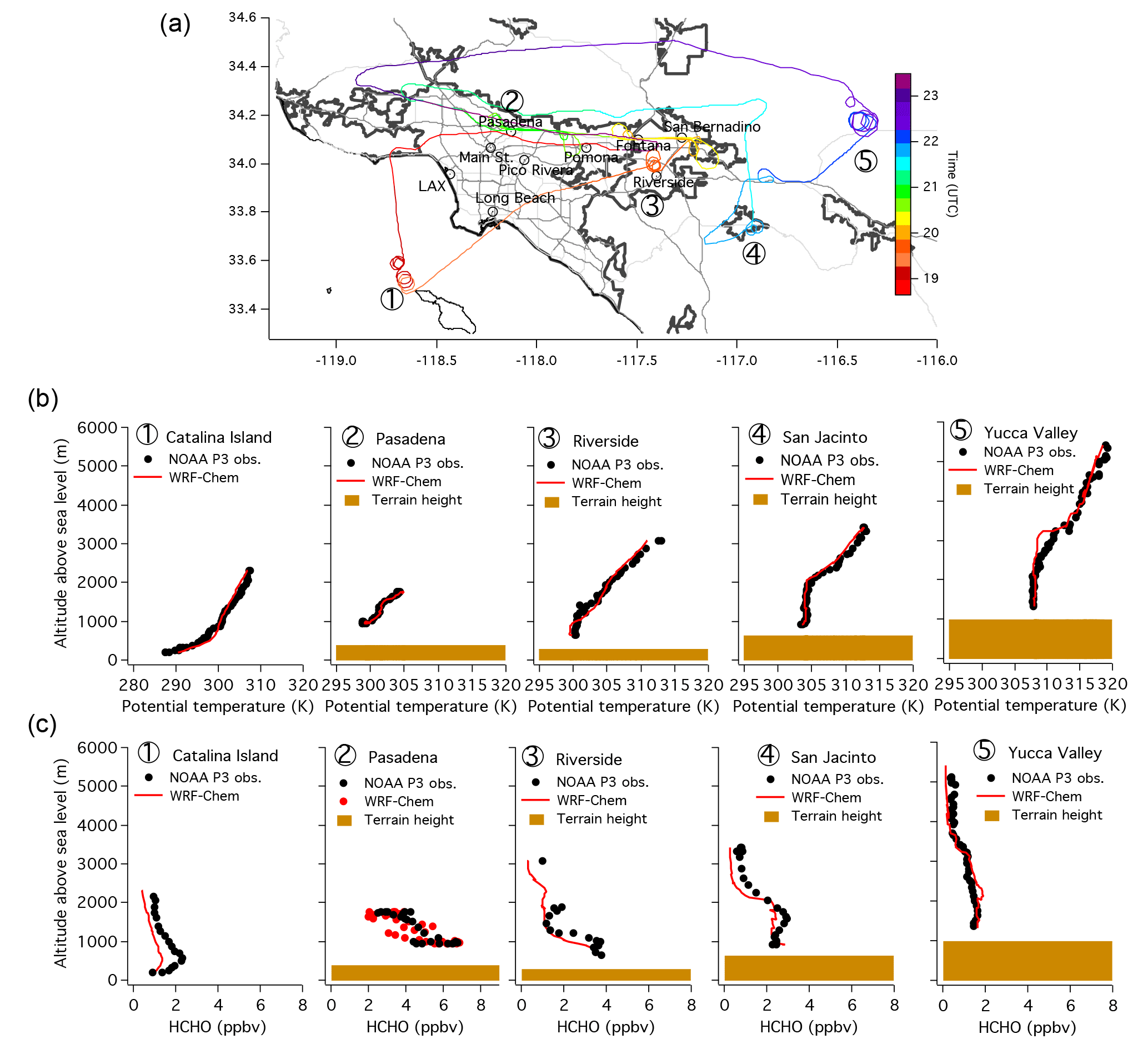
Figure 2The flight path of NOAA WP-3 (a) and the spatial distribution of vertical profiles of aircraft observed and model simulated potential temperature (b) and HCHO (c) in the LA Basin on 4 May 2010. The black filled circles and red solid lines/symbols represent the observations and model results, respectively.
3.1 Observed and simulated HCHO
In order to use the model HCHO profiles for AMF calculations and to explore impacts of fine-resolution a priori information on the retrievals, they should be reasonably good representations of the real atmospheric profiles. Therefore, we evaluate WRF-Chem HCHO simulations with the ground-based LP-DOAS data and aircraft PTR-MS observations. Figure 1 shows diurnal variations of the near-surface LP-DOAS HCHO observations and model results using various emission inventories on weekdays and weekends. The model results using either the top-down VOC emission estimates based on Borbon et al. (2013; red lines) and the NEI05 (Kim et al., 2016; blue lines) agree with the observations best. The model underestimates the LP-DOAS HCHO observations when we ignore the biogenic VOC emissions or adopt the most-up-to-date VOC inventory for year 2010 (NEI11, described in Ahmadov et al., 2015), with its lower anthropogenic alkene emissions than those from the NEI05 and top-down approaches. Maximum observed and modeled HCHO mixing ratios in Pasadena are about 4 ppbv during weekdays or 5 ppbv during weekends. During the weekends, faster photochemistry due to lower NOx emissions causes higher ozone and HCHO mixing ratios (Pollack et al., 2012; Kim et al., 2016).
Figure 2 shows the vertical profiles of potential temperature and HCHO mixing ratio from the aircraft observations and model results in the LA Basin on 4 May 2010. The potential temperature profiles in the model agree with the observations and help to characterize different vertical mixing regimes: a stable boundary layer near Catalina Island and the growth of the convective boundary layer from the LA urban cores eastward to the desert on the east side of the basin. Similarly, the WRF-Chem HCHO profiles are in good agreement with the WP-3 PTR-MS observations. The convective boundary layer develops mainly by buoyancy forcing during daytime and leads to well-defined boundary layer heights (or mixing heights) ranging from a few hundred meters to several kilometers and well-mixed vertical profiles of potential temperature and scalars. Meanwhile, stable boundary layers are characterized by a shallow boundary layer (boundary layer height of maximum a few hundred meters), a positive vertical gradient of potential temperature near the surface, and poorly mixed vertical profiles of scalars because of weak turbulent mixing that frequently occurs over the ocean or during nighttime. Overall, our model results agree with the observations from the aircraft and ground-based observations; therefore, it is reasonable to use the model HCHO profiles as inputs to VLIDORT and to examine the AMF results from this RT model.
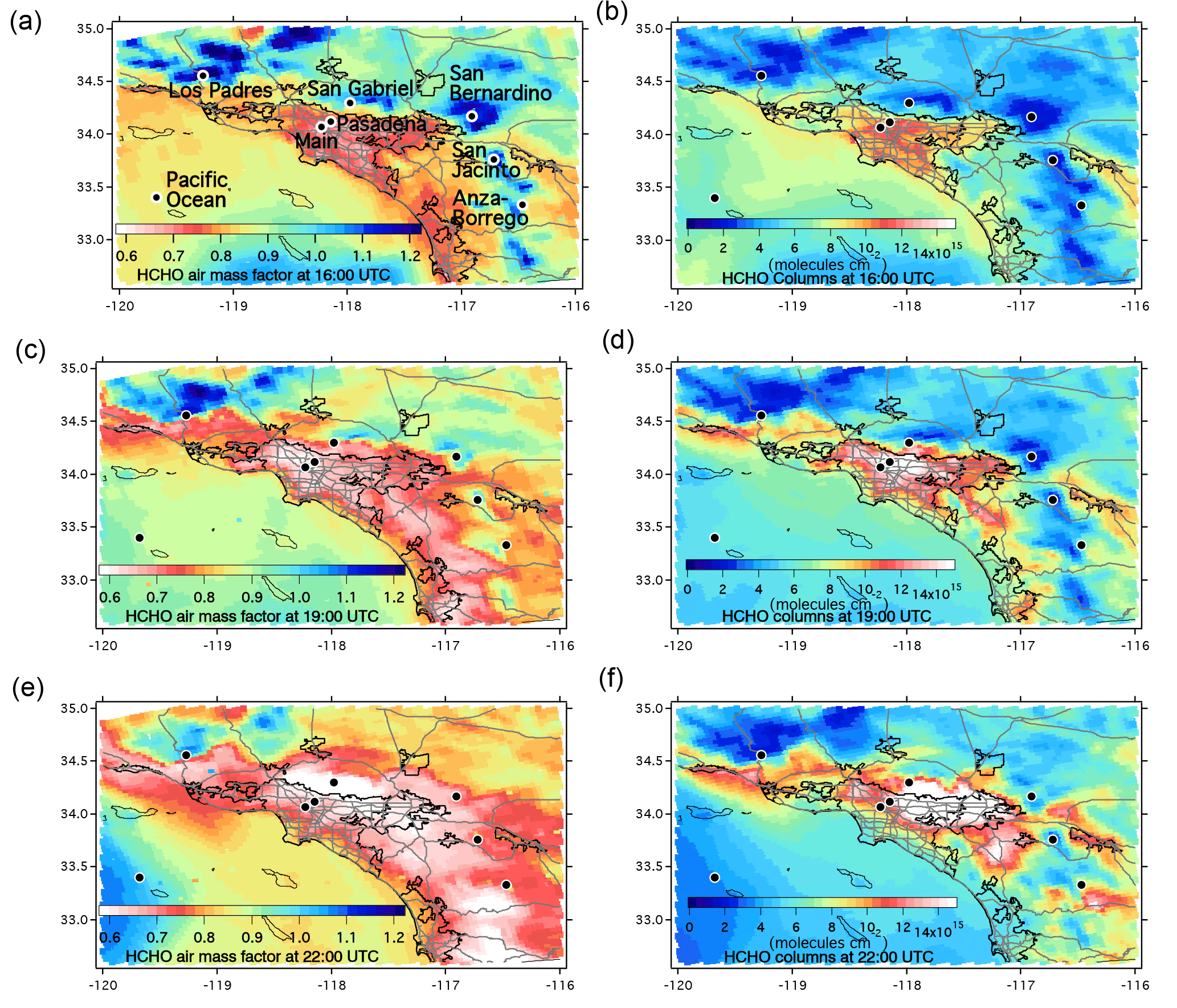
Figure 3The spatial distributions of air mass factors from the radiative transfer model calculations (a, c, e) and HCHO columns (b, d, f) in the LA Basin at 16:00 UTC (a, b), 19:00 UTC (c, d), and 22:00 UTC (e, f) on 4 May 2010. The black filled circles are included as points of further investigations, representing background, urban cores, and downwind regions.
3.2 Spatial distribution of the AMF and sensitivity to a priori profiles at different times of day
The spatial distribution of the VLIDORT HCHO AMF using the WRF-Chem profiles at 4 km × 4 km resolution at different times of day on 4 May 2010 is shown in Fig. 3. The AMF ranges from 0.6 to 1.2 within the LA Basin and in the nearby coastal areas. The AMF values are 0.6–0.7 in the urban cores. In contrast, for high mountains such as the Los Padres National Forest located in the northwestern part of the basin, the AMF is greater than 1. Above the Pacific Ocean near the coast, the AMF is about 0.9–1. These results are similar to the AMF calculations by Palmer et al. (2001); they obtained AMF = 0.71 in Tennessee, where high isoprene levels are seen in the boundary layer, and AMF = 1.1 over the North Pacific. The AMF values calculated by Palmer et al. (2001) resulted in Global Ozone Monitoring Experiment (GOME) measurements that were ∼ 35 % less sensitive to the HCHO column (or 35 % smaller total AMF) over Tennessee than over the North Pacific. Palmer et al. (2001) also noted small AMF values over California, which they attributed to a shallow boundary layer resulting from strong subtropical subsidence combined with a strong surface source of HCHO from biogenic hydrocarbons. Our study agrees with this finding, except that both anthropogenic and biogenic VOCs contribute to high formaldehyde in the LA Basin (Fig. 1). General features of the AMF distribution in the area do not change significantly when a constant surface pressure is used in the RT simulations (see Supplement Figs. S1 and S2). A total of 82 % (99 %) of the area shows the differences of the AMF less than 5 % (10 %). The direct influence of complex terrain height on the AMF is small. Similarly, the spatial pattern was not strongly affected by the currently available bottom-up emission inventory used to generate the WRF-Chem HCHO profiles in our study (see Supplement Figs. S1 and S2). A total of 95 % (98 %) of the area shows the differences of the AMF less than 5 % (10 %). The impact of the bottom-up emission inventory was larger in Barkley et al. (2012) when various isoprene emission inventories over tropical South America were included in the satellite HCHO retrievals: in general, the difference in the HCHO columns was ±20 % and for individual locations it was up to ±45 %. Thus, the role the bottom-up emission inventory play in the AMF calculation varies depending on the quality (accuracy) of the emission inventories and their impacts on the profile shapes.
As mentioned above, the most operational HCHO retrievals adopted global model results at roughly 1–3∘ grid size as a priori profile, which are ∼ 1000 times as large as the spatial resolution in our study (4 km × 4 km). For the domain of interest in this study, the global model has just a few profiles. Here we compare the AMF from global model results (2∘ latitude × 2.5∘ longitude resolution) as a priori in the SAO OMI formaldehyde retrieval (González Abad et al., 2015) with the AMF from this study for the LA Basin and discuss more on the spatial resolution effect. In contrast to the AMF in this study as in Fig. 3, the AMF in the SAO OMI formaldehyde retrieval does not vary much in the basin and is close to 1 (see Fig. S3 in the Supplement for details). The average of the AMF from the OMI SAO product for the domain (33.5–34.5∘ N, 117–118.5∘ W) is 1.12 while the same domain average of the AMF from this study is 0.76. If the AMF in this study is used, the HCHO column can increase by 47 % on the domain average (up to ∼ 100 % at a finer scale), compared with the OMI HCHO column. The vertical HCHO profile in the OMI SAO product is almost a constant in the domain while the model profile at 4 km × 4 km resolution varies substantially. We will discuss the spatial resolution effect on the intensity of HCHO plumes in depth later.
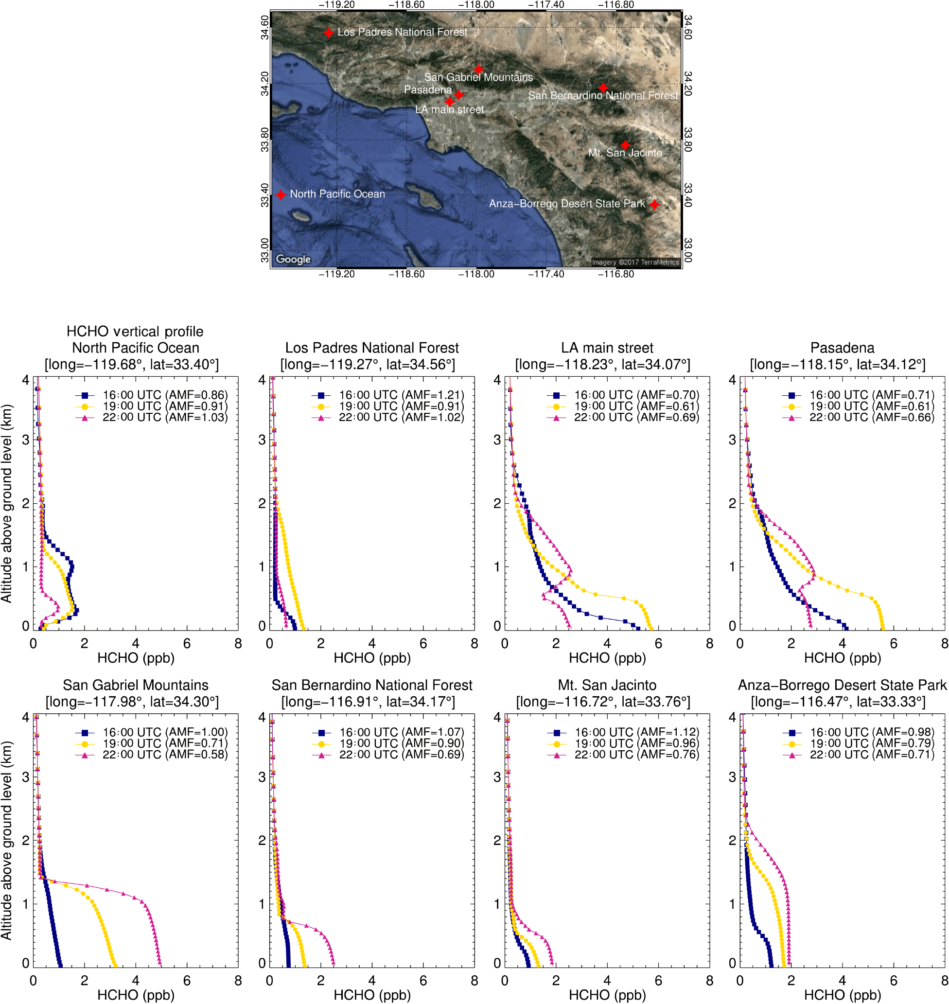
Figure 4Vertical profiles of HCHO are shown for various points of interest (red symbols on a Google map). Blue, orange, and magenta lines represent 16:00, 19:00, and 22:00 UTC (or 09:00, 12:00, 15:00 PDT), respectively, on 4 May 2010. The altitude above ground level is shown. The same plot with the unit of molecules cm−3 is shown in the Supplement.
Geostationary satellites such as TEMPO (Fishman et al., 2012; Zoogman et al., 2017), GEMS (Kim and the GEMS Team, 2012), and Sentinel-4 (Ingmann et al., 2012; Veihelmann et al., 2015) are expected to provide diurnally varying information about tropospheric pollution during daytime. It is, therefore, useful to investigate if diurnally varying a priori profile information is needed for accurate retrievals of satellite-based HCHO columns. Figure 3 shows the spatial distribution of the VLIDORT HCHO AMF using the WRF-Chem profiles at 16:00, 19:00, and 22:00 UTC (equivalent to 09:00, 12:00, 15:00 Pacific Daylight Time, PDT, respectively) and HCHO columns. Overall, similar patterns of the AMF distribution are shown at all times: low AMFs in the urban cores and high AMFs in the area of the Los Padres National Forest located in the northwestern region of the basin. However, there are noticeable diurnal changes in the AMFs over the high terrain east and northeast of downtown LA and over the Pacific Ocean near the coast, due to changing photochemical production and destruction and transport of HCHO throughout the day (Fig. 3). Overall, minimum AMF values are reduced between morning and afternoon as HCHO is photochemically produced. At 15:00 PDT, AMF values < 0.6 (the white shading in Fig. 3) occur in the mountainous regions, including the San Gabriel Mountains, San Bernardino National Forest, Mt. San Jacinto, and Anza-Borrego Desert State Park. Onshore transport of photochemically produced HCHO plumes from downtown LA to the mountains occurs in the afternoon (see HCHO columns in Fig. 3).
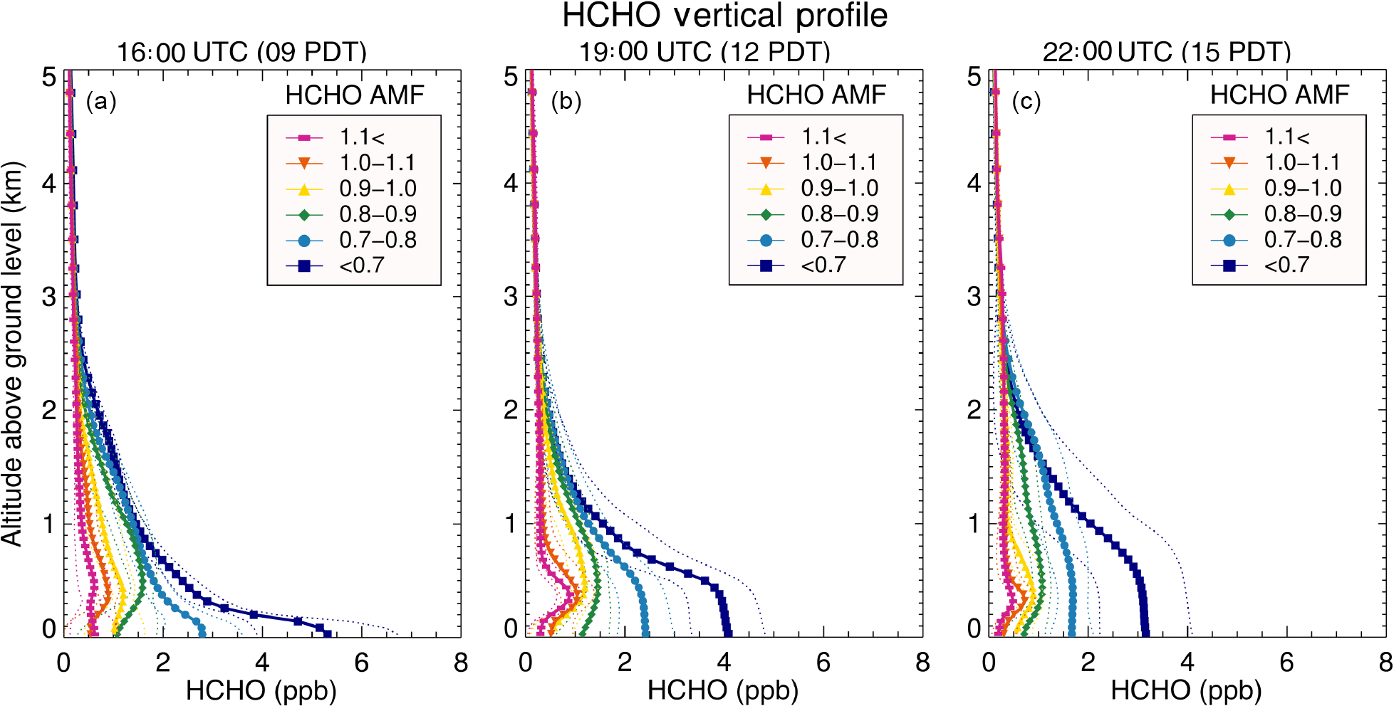
Figure 5Vertical profiles of HCHO averaged for the AMF value intervals (as in legends) at 16:00, 19:00, and 22:00 UTC (a–c) are displayed. Thick lines with symbols are for averages and thin dotted lines are for 1 standard deviation values. The altitude above ground level is shown. The same plot with the unit of molecules cm−3 is shown in the Supplement.
Figure 4 shows vertical distributions of the model HCHO mixing ratios at several locations in the LA Basin and the Pacific Ocean for the AMF values at different times of day (see Fig. S4 in the Supplement for the plots with number density unit, molecules cm−3). Over the Pacific Ocean, the HCHO mixing ratio is small near the surface and more abundant at higher altitudes. The AMF over the ocean increases with time from 0.86 at 09:00 PDT to 1.03 at 15:00 PDT as the HCHO mixing ratio decreases with time, probably due to transport of the plume from the ocean to the inland area (see Supplement Fig. S5 for detailed analyses). Over the land, the HCHO mixing ratio is higher in the boundary layer than in the free atmosphere. In the Los Padres National Forest, where the highest AMF (0.91–1.21) occurs, the boundary layer grows with time, but the mixing ratio of HCHO is small (< 1 ppbv). In Pasadena and at the LA Main St. site, the boundary layer heights and HCHO mixing ratios increase from 09:00 to 12:00 PDT. The maximum HCHO value in the boundary layer is about 6 ppbv. The HCHO in the boundary layer decreases at 15:00 PDT, but mixing ratios above the boundary layer (> 1 km) increase due to the upper-level easterly transport of the HCHO plumes. Consequently, the AMF decreases from 0.7 at 09:00 PDT to 0.6 at 12:00 PDT and then increases to 0.7 at 15:00 PDT, due to an enhanced sensitivity to increased upper-level HCHO mixing ratios. For these urban core sites, the HCHO AMF ranges from 0.6 to 0.7. In the San Gabriel Mountains, San Bernardino National Forest, and Mt. San Jacinto, the boundary layer height is well defined and shallow and does not change significantly throughout the day. However, the AMF values change substantially (decreasing by ∼ 40 %) throughout the day over these locations; this is likely because HCHO mixing ratios increase between morning and afternoon, mainly due to transport and formation of the plumes originating from urban core regions. The AMF at Anza-Borrego Desert State Park decreases with time from 0.96 at 09:00 PDT to 0.71 at 15:00 PDT due to increasing HCHO mixing ratios, in spite of the increase in boundary layer height. These findings highlight the importance of using time-varying, high-spatial-resolution a priori profile information for the accurate retrieval of geostationary HCHO measurements.
We extended this analysis in Fig. 5, where for ranges of the HCHO AMF (e.g., 1.0 < AMF < 1.1) across the model domain, the model HCHO profiles are averaged and plotted at the three times (09:00, 12:00, and 15:00 PDT; see Fig. S6 in the Supplement for the plots with number density unit, molecules cm−3). Each plot shows that the AMF values are smaller when the HCHO mixing ratios are higher near the surface. At 12:00 and 15:00 PDT, as expected, the profiles have more well-mixed shapes for deeper vertical layers. The dependence of the AMF value on the profile shape is similar at each time of day: the higher AMF is related to lower HCHO mixing ratios (or number densities) in the atmospheric boundary layer (up to 1–3 km a.g.l.). More quantitative analysis is shown below.
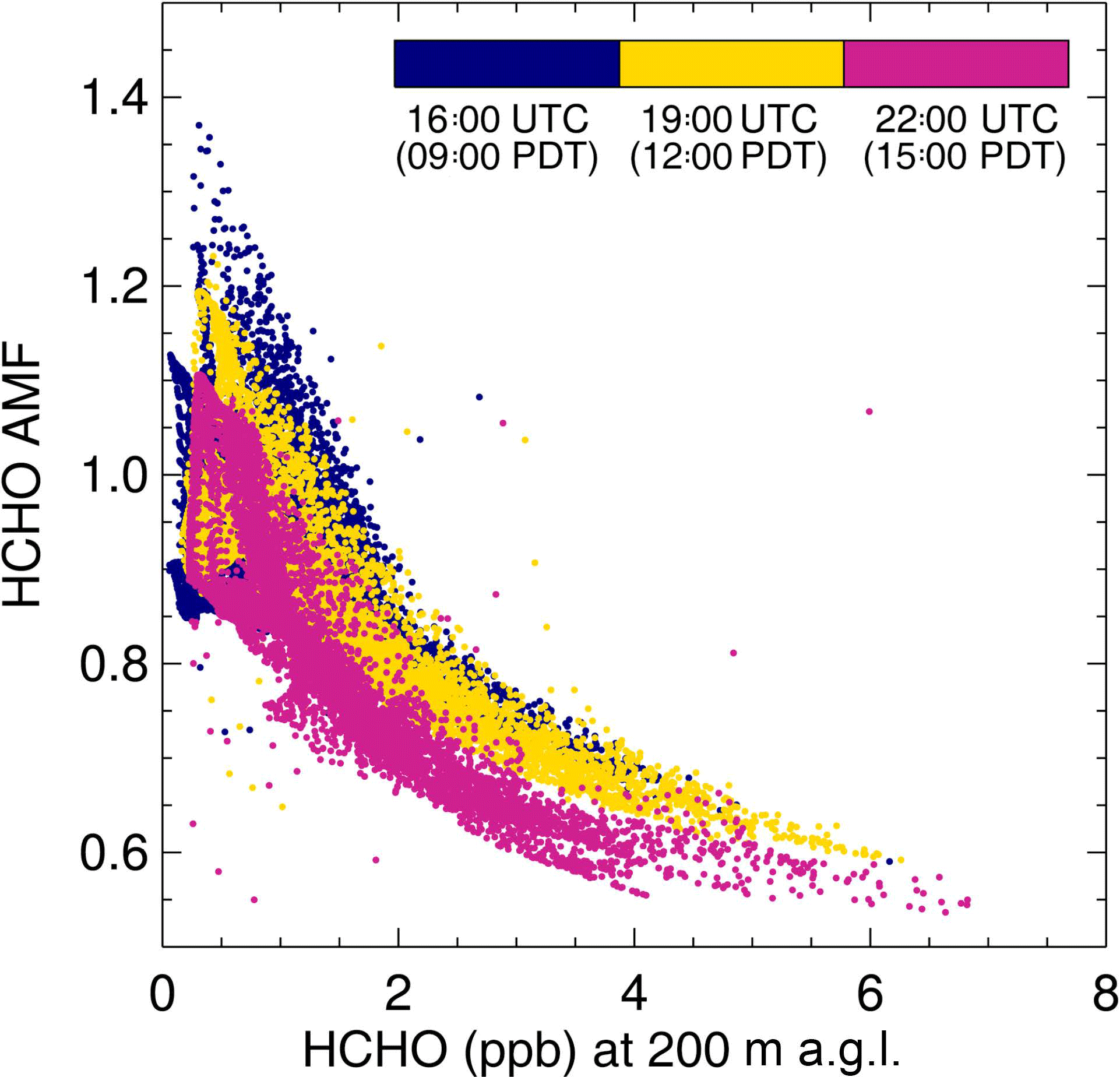
Figure 6The relationship between the AMF and model HCHO volume mixing ratio is demonstrated. Different colors denote different times. The HCHO mixing ratio at ∼ 200 m a.g.l. is plotted. The same plot with the unit of molecules cm−3 is shown in the Supplement.
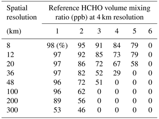
Using all available data points, we investigate the relationship between the AMF and the HCHO mixing ratio at 200 m in the boundary layer at different times of day in Fig. 6 (see Fig. S7 in the Supplement for the plots with number density unit, molecules cm−3). The plot illustrates that as the HCHO mixing ratio increases, the AMF decreases. At all times investigated, the AMF is anti-correlated with HCHO mixing ratio (or number density). Correlation coefficients between the AMF and HCHO mixing ratio are −0.68, −0.85, and −0.84 at 16:00 (09:00), 19:00 (12:00), and 22:00 (15:00) UTC (PDT). In general, AMF values decrease from morning to late afternoon. The AMF values are reduced substantially for the HCHO mixing ratio of 2, 3, and 4 ppb. Therefore, it is useful to examine if the HCHO mixing ratios of 2, 3, and 4 ppb or higher can be captured at coarser spatial resolutions. Figure 7 demonstrates a scatter of HCHO concentrations at 4 km × 4 km resolution on a coarser grid from 8 to 300 km. Here the values for coarse grids are generated from the spatial averages of the original model results at 4 km resolution in this study. A scatter of concentrations is getting larger at a spatial grid size ≥ 20 km. For example, the concentration at 4 km resolution varies from 1 to 6 ppb while that at 100 km resolution is about 2 ppb. Table 1 summarizes the efficiency of capturing the plumes that have greater HCHO mixing ratio than the reference values for each spatial grid resolution. Of particular importance are the reference values of 2, 3, and 4 ppb, for which the AMF is greatly reduced. Table 1 indicates that the grid size ≤ 12 km can capture the plumes of HCHO volume mixing ratio (VMR) > 4 or 5 ppb at 4 km by more than 70 %. If the grid size is 8 km, the plumes of 1–5 ppb are detected by ∼ 80 %. If the grid size is greater than 100 km, it does not capture the plume of VMR > 2 ppb at this urban location. Thus, the AMF using the coarse resolution ≥ 100 km is about 1 because of low concentration < 2 ppb. Currently the typical spatial resolution of regional-scale models for the viewing domain of the geostationary satellites (e.g., air quality forecast models for the US) is 12–30 km in each latitude and longitude direction. Our recommendation is to select the resolution as close as 4 km. Since the model simulation at 4 km resolution is computationally expensive for the current geostationary satellite viewing domain and all of the high-quality input data to the model are not readily available at this resolution (e.g., emission inventory), the model simulations at 8–12 km resolution are recommended to test and improve the model simulations and finally acquire the a priori profile for the next generation environmental geostationary satellite retrievals if computing resources are available.

Figure 7Comparison of HCHO mixing ratios at 4 km × 4 km resolution with mixing ratios at coarser resolutions of (a) 8 km × 8 km, (b) 12 km × 12 km, (c) 20 km × 20 km, (d) 36 km × 36 km, (e) 48 km × 48 km, (f) 100 km × 100 km, (g) 200 km × 200 km, and (h) 300 km × 300 km. The one-to-one line is shown in black.
Table 1Percentage (%) of intense HCHO plumes retained as the spatial resolution is changed from 4 km. Each column shows the fraction of the plumes retained at coarser resolutions. Here the plume is defined by the area in which the HCHO mixing ratio is greater than the reference HCHO volume mixing ratio (VMR) (1–6 ppb) at 4 km resolution. For example, the second column shows how much area at 8–200 km resolution has a HCHO VMR > 1 ppb when compared with the area with VMR > 1 ppb at 4 km resolution. Similarly, the last column shows how often a model HCHO VMR is greater than 6 ppb at 8–200 km resolution compared with the same plume of VMR > 6 ppb at 4 km resolution; all coarser resolutions (8–200 km) fail to capture this most intense plume. Only model HCHO results at 200 m above ground level at 19:00 UTC (12:00 PDT) are used. The areas with HCHO VMRs greater than 1, 2, 3, 4, 5, or 6 ppb are 92 800, 29 136, 12 832, 4256, 848, or 64 km2, respectively, in the original simulations at 4 km resolution. The area of the domain is 143 856 km2.
For UV-VIS retrievals, it is well known that the vertical profile shape affects the value of the AMF. Our study suggests a strong anti-correlation between the absolute concentration and the AMF: the AMF is low in the area of intense HCHO plumes. The changes in the absolute HCHO concentrations in the boundary layer (altitude < 1–3 km a.g.l.) strongly modify profile shapes, which in turn affect the AMF substantially. To understand the importance of the absolute magnitude of HCHO mixing ratios within the context of the mathematical formula of the AMF used, we examine shape factor, scattering weight function, and AMF quantitatively. According to Palmer et al. (2001), the AMF is expressed as
Here AMFG is a geometric air mass factor that is a function of solar zenith angle and satellite viewing angle, w(z) is a scattering weight that is associated with the sensitivity of the backscattered spectrum to the abundance of the absorber at altitude z, and Sz(z) is a vertical shape factor for the absorber representing a normalized vertical profile of number density. The vertical shape factor is defined as
where n(z) is the number density (molecules cm−3) at altitude z and Ωv is the vertical column density or column (molecules cm−2) of HCHO. In this paper, the AMF in Eq. (1) is vertically integrated to the top of the model domain that is roughly the top of the troposphere or above. Therefore, the AMF here is the tropospheric AMF. To understand the sensitivity of the AMF on the vertical distribution, we also define ΔAMFi, a discrete increment of the AMF for each model layer.
where i is an index representing the vertical grids, Δzi is the layer depth for the grid i, and .

Figure 8Vertical profiles of (a) shape factor and scattering weight and (b) ΔAMFi (discrete increment of the AMF) at the North Pacific Ocean, San Gabriel Mountains, and Anza-Borrego Desert State Park. Scattering weights multiplied by the geometric AMF are shown. Dashed lines and solid lines with symbols in the left panel denote the scattering weight and shape factor, respectively. Total (or tropospheric) AMF values are shown in legends in panel (b).
In Fig. 8, the vertical shape factor in Eq. (2), the scattering weight (multiplied by geometric AMF), and ΔAMFi are plotted as a function of height over the North Pacific Ocean, San Gabriel Mountains, and Anza-Borrego Desert State Park at 16:00, 19:00, and 22:00 UTC (see Fig. 4 for the locations of these sites). The differences in the shape factor over the North Pacific Ocean are clear at altitudes > ∼ 1000 m: the shape factor values at 22:00 UTC are larger than those at 16:00 and 19:00 UTC. In contrast, the HCHO column at 22:00 UTC is smaller than those at 16:00 and 19:00 UTC over the ocean (Fig. 4). As the column density value decreases, the shape factor above ∼ 1000 m becomes larger and causes higher ΔAMFi and (tropospheric) AMFs, because a column density value is used as a normalization parameter for a shape factor. In order words, the satellite measurement is more sensitive to the profile at 22:00 UTC than that at 16:00 UTC at this point over the Pacific Ocean.
For the San Gabriel Mountains site, the HCHO is confined below ∼ 1400 m at 16:00, 19:00, and 22:00 UTC (there are no significant changes in boundary layer height during this time period) and its mixing ratio increases with time (Fig. 4). The shape factor at 19:00 and 22:00 UTC is higher than that at 16:00 UTC below ∼ 1400 m altitude (Fig. 8, middle row). However, above this height, the shape factor and ΔAMFi decrease with time: both are largest at 16:00 UTC and smallest at 22:00 UTC. The tropospheric AMF follows ΔAMFi above ∼ 1400 m and also decreases with time from 1 to 0.58. Thus, the satellite measurement is more sensitive to the profile at 16:00 UTC than that at 22:00 UTC in this mountainous area. The plot over the San Gabriel Mountains area illustrates that not only boundary layer height, but also the absolute magnitude of HCHO influences the AMF value.
The Anza-Borrego Desert State Park represents an example of a case in which both boundary layer height and HCHO mixing ratio increase with time (Figs. 4 and 8, bottom row). In the case of the lowest boundary layer height (at 16:00 UTC), the AMF is largest (AMF = 0.98). When the boundary layer height is the highest among the three time periods (at 22:00 UTC), the AMF is smallest (AMF = 0.71). For Anza-Borrego Desert State Park, the total column or near-surface HCHO mixing ratio affect the shape factor, which in turn leads to an AMF that is inversely proportional to the total column or near surface HCHO mixing ratio. As shown in Fig. 8, the shape factor and ΔAMFi above the boundary layer decrease with time, which causes a decrease in the tropospheric AMF with time.
In summary, the absolute value of the column or near-surface mixing ratio of HCHO affects the shape factor as a normalization factor, in particular the value in the free troposphere (above boundary layer), which dominates the tropospheric AMF. When the HCHO mixing ratio is low in the boundary layer, the relative importance of the absorber in the free troposphere increases. Conversely, when the HCHO mixing ratio is high in the boundary layer, the relative importance of absorber in the free atmosphere decreases. Our result suggests that a representation of the HCHO AMF using accurate fine-resolution a priori profile information is critical to identify HCHO plumes and to place better constraints on VOC emissions.
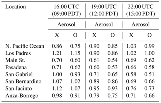
Although the focus of this paper is on the shape factor, we also investigate the impacts of aerosol loading on the AMF for the eight sites shown in Fig. 4. When the aerosol optical properties from the model results are incorporated in our RT model calculations, the AMF is reduced by ∼ 10 % at the N. Main St. and Pasadena sites and by <10 % at other sites (Table 2). The aerosol optical depth, single scattering albedo, and asymmetry factor calculated from the model results for the eight sites are about 0.5, 0.9, and 0.7, which is close to the values suggested as the most probable atmospheric conditions in the LA Basin (see Table 4 in Baidar et al., 2013). Because the model aerosol results were not thoroughly evaluated and optimized and only eight sites were tested, the analysis of aerosol impact in this study is limited. It is possible that some of the simulated aerosol components are overestimated, because the emission inventory is not fully up to date for primary aerosol emissions and aerosol precursor gases (e.g., overestimations of black carbon and SO2 by a least a factor of 3). Meanwhile, the AMF changes from the values at 16:00 UTC (09:00 PDT) due to diurnal variations in a priori profile shape range from −40 to 20 % (Table 2). It is likely that the impact of aerosols on the AMF is relatively small when compared with the impact of the profile shape factor examined in this study for the LA Basin. De Smedt et al. (2015) and Wang et al. (2017) also reported the importance of a priori profile shapes for an improvement of satellite-based HCHO retrievals in Beijing, Xianghe, and Wuxi in China. Kwon et al. (2017) demonstrated that the impact of aerosol loading on the HCHO AMF can be large over East Asia, in particular, for a case of Asian dust transport, in contrast to our study for the LA Basin.
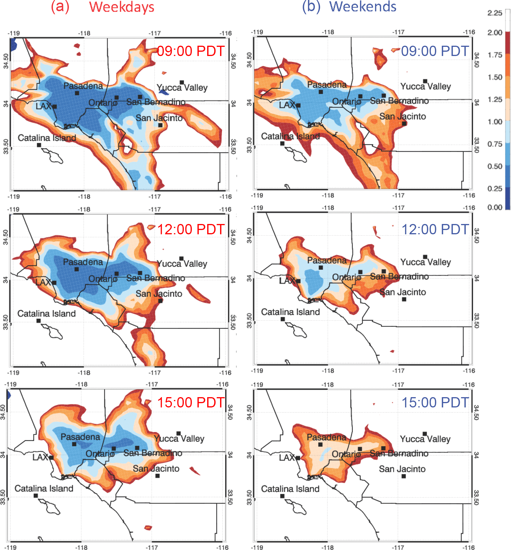
Figure 9Spatial distributions of the ratios of the model HCHO column to NO2 column during weekdays (a) and weekends (b) at 09:00, 12:00, and 15:00 PDT for May–June 2010. The light pink to red colored contours denote the area under the NOx-limited chemical regime.
Table 2Summary of air mass factors at eight locations at 16:00–22:00 UTC (09:00–15:00 PDT). The results without/with aerosols impacts are also shown.
3.3 Air quality application of fine-resolution geostationary HCHO columns
In this section, we illustrate the application of future geostationary HCHO retrievals to the study of air quality, by using the WRF-Chem HCHO columns as a proxy for satellite data. Figure 9 demonstrates the distribution of the ratio of HCHO to NO2 tropospheric vertical columns from the WRF-Chem model in the LA Basin at different times of day and on weekdays and weekends for May–June 2010. For more information about the model NO2 columns, refer to Kim et al. (2016).
Ratios of HCHO to NO2 columns provide critical information about chemical regimes relevant to controlling ozone pollution (Martin et al., 2004a; Jin et al., 2017). In Fig. 9, the light blue to blue contours (HCHO/NO2 < 1) represent VOC-sensitive (or VOC-limited) ozone production regimes, while the pink to the red contours (HCHO/NO2 > 1) denote NOx-sensitive regimes. During weekdays in 2010, most of the LA Basin is in the VOC-sensitive regime, where a reduction in NOx emissions can cause an increase in O3. In the late afternoon during weekends, the broad polluted area becomes NOx sensitive, so that NOx reductions lead to O3 decreases.
Figure 10 shows 2000–2010 trends in surface O3 from monitors in Pasadena and San Bernardino. During this decade, NOx emissions were decreasing in the LA Basin, largely due to better control of motor vehicle pollution (McDonald et al., 2012). On weekdays during this decade, there was not a declining trend in surface O3 in Pasadena, while O3 increased in San Bernardino. In contrast, on weekends, O3 decreased between 2000 and 2010 in both Pasadena and San Bernardino. These observed O3 trends are consistent with analyses of the ratio of HCHO to NO2 columns and their representation of VOC/NOx sensitivity, shown in Fig. 10. Baidar et al. (2015) found that the spatial extent and the trend of higher O3 during weekends than weekdays had decreased in the LA Basin because of the increased tendency of lower O3 during hot weekends, especially after the 2008 economic recession.
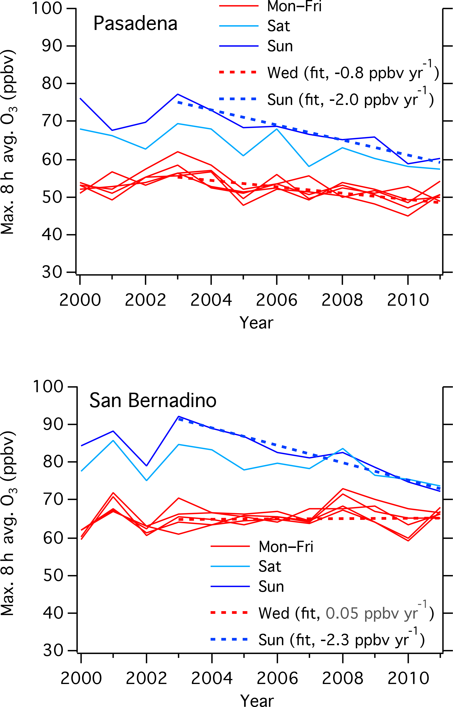
Figure 10Decadal O3 trends in Pasadena and San Bernardino during weekdays (red) and weekends (blue) are shown. The linear least square fits of O3 for Wednesday and Sunday are plotted in dashed lines.
The polar-orbiting satellite instruments that are currently available do not provide diurnally varying information on HCHO/NO2 columns and VOC/NOx sensitivities, because these measurements are made once a day in either the morning or early afternoon. The discussion above makes it clear that future geostationary satellite HCHO and NO2 columns will provide useful information about photochemical ozone regimes that could be used to evaluate pollution control policies.
Our tests of the sensitivity of the HCHO AMF to several factors confirm the importance of a priori HCHO profile shapes. Our study reveals that the AMF is very sensitive to the absolute HCHO mixing ratio (or number density) in the boundary layer. Therefore, the absolute magnitude of HCHO concentration in the boundary layer is an essential factor in determining the AMF. For the coastal LA Basin megacity studied in this work, the AMF values are inversely proportional to the magnitude of the HCHO mixing ratios in the boundary layer. Furthermore, the AMF over land is lower in the late afternoon (15:00 PDT) than in the morning (09:00 PDT), because of increasing HCHO mixing ratios throughout the day. Therefore, diurnal updates and fine spatial resolution a priori profile shapes are likely to improve the retrievals of satellite-based HCHO columns.
The spatial distributions of fine-scale model HCHO columns in the LA Basin show hotspots in downtown LA around noon and enhancement and transport of the plumes to the eastern part of the basin in the late afternoon. The ratio of HCHO to NO2 columns during weekdays and weekends provides information on the chemical regimes relevant to ozone formation at various locations and times in the basin. Future geostationary satellites (e.g., TEMPO) may provide similar information, which could be used to assess the effectiveness of existing pollution controls and could help in planning or revising air pollution control policies.
The WRF-Chem (Weather Research and Forecasting-Chemistry) model (Grell et al., 2005) used in this study is available at http://www2.mmm.ucar.edu/wrf/users/download/get_source.html (last access: 28 May 2018). We acknowledge use of the MOZART-4 global model output available at http://www.acom.ucar.edu/wrf-chem/mozart.shtml (last access: 28 May 2018). The CalNex field campaign data are available at http://www.esrl.noaa.gov/csd/projects/calnex/ (last access: 28 May 2018).
The supplement related to this article is available online at: https://doi.org/10.5194/acp-18-7639-2018-supplement.
The authors declare that they have no conflict of interest.
The NOAA Health of Atmosphere program, the NASA ROSES ACMAP (NNH14AX01I),
and the NASA GEO-CAPE mission pre-formulation study (NNH13AW31I) supported this
research. This subject was supported by the Korea Ministry of Environment (MOE) as the Public Technology Program based on
Environmental Policy (2017000160001). The authors thank Gonzalo González Abad and Kelly Chance at Harvard
SAO and Hyo-Jung Lee at Pusan National University.
Edited by: Michel Van Roozendael
Reviewed by: two anonymous referees
Ahmadov, R., McKeen, S., Trainer, M., Banta, R., Brewer, A., Brown, S., Edwards, P. M., de Gouw, J. A., Frost, G. J., Gilman, J., Helmig, D., Johnson, B., Karion, A., Koss, A., Langford, A., Lerner, B., Olson, J., Oltmans, S., Peischl, J., Pétron, G., Pichugina, Y., Roberts, J. M., Ryerson, T., Schnell, R., Senff, C., Sweeney, C., Thompson, C., Veres, P. R., Warneke, C., Wild, R., Williams, E. J., Yuan, B., and Zamora, R.: Understanding high wintertime ozone pollution events in an oil- and natural gas-producing region of the western US, Atmos. Chem. Phys., 15, 411–429, https://doi.org/10.5194/acp-15-411-2015, 2015.
Alicke, B., Platt, U., and Stutz, J.: Impact of nitrous acid photolysis on the total hydroxyl radical budget during the Limitation of Oxidant Production/Pianura Padana Produzione di Ozono study in Milan, J. Geophys. Res.-Atmos., 107, 8196, https://doi.org/10.1029/2000jd000075, 2002.
Baidar, S., Oetjen, H., Coburn, S., Dix, B., Ortega, I., Sinreich, R., and Volkamer, R.: The CU Airborne MAX-DOAS instrument: vertical profiling of aerosol extinction and trace gases, Atmos. Meas. Tech., 6, 719–739, https://doi.org/10.5194/amt-6-719-2013, 2013.
Baidar, S., Hardesty, R. M., Kim, S.-W., Langford, A. O., Oetjen, H., Senff, C. J., Trainer, M., and Volkamer, R.: Weakening of the weekend ozone effect over California's South Coast Air Basin, Geophys. Res. Lett., 42, 9457–9464, https://doi.org/10.1002/2015GL066419, 2015.
Barkley, M. P., Kurosu, T. P., Chance, K., De Smedt, I., Roozendael, M. V., Arneth, A., Hagberg, D., and Guenther, A.: Assessing sources of uncertainty in formaldehyde air mass factors over tropical South America: Implications for top-down isoprene emission estimates, J. Geophys. Res.-Atmos., 117, D13304, https://doi.org/10.1029/2011JD016827, 2012.
Barth, M. C. Kim,, S.-W., Skamarock, W. C., Stuart, A. L., Pickering, K. E., and Ott, L. E.: Simulations of the redistribution of formaldehyde, formic acid, and peroxides in the 10 July 1996 Stratospheric-Tropospheric Experiment: Radiation, Aerosols, and Ozone deep convection storm, J. Geophys. Res.-Atmos., 112, D13310, https://doi.org/10.1029/2006JD008046, 2007.
Boersma, K. F., Eskes, H. J., and Brinksma, E. J.: Error analysis for tropospheric NO2 retrieval from space, J. Geophys. Res.-Atmos., 109, D04311, https://doi.org/10.1029/2003JD003962, 2004.
Borbon, A., Gilman, J. B., Kuster, W. C., Grand, N., Chevaillier, S., Colomb, A., Dolgorouky, C., Gros, V., Lopez, M. Sarda-Esteve, R., Holloway, J., Stutz, J., Petetin, H., McKeen, S., Beekmann, M., Warneke, C., Parrish, D. D., and de Gouw, J. A.: Emission ratios of anthropogenic volatile organic compounds in northern mid-latitude megacities: Observations versus emission inventories in Los Angeles and Paris, J. Geophys. Res.-Atmos., 118, 2041–2057, https://doi.org/10.1002/jgrd.50059, 2013.
De Smedt, I., Stavrakou, T., Hendrick, F., Danckaert, T., Vlemmix, T., Pinardi, G., Theys, N., Lerot, C., Gielen, C., Vigouroux, C., Hermans, C., Fayt, C., Veefkind, P., Müller, J.-F., and Van Roozendael, M.: Diurnal, seasonal and long-term variations of global formaldehyde columns inferred from combined OMI and GOME-2 observations, Atmos. Chem. Phys., 15, 12519–12545, https://doi.org/10.5194/acp-15-12519-2015, 2015.
De Smedt, I., Theys, N., Yu, H., Danckaert, T., Lerot, C., Compernolle, S., Van Roozendael, M., Richter, A., Hilboll, A., Peters, E., Pedergnana, M., Loyola, D., Beirle, S., Wagner, T., Eskes, H., van Geffen, J., Boersma, K. F., and Veefkind, P.: Algorithm theoretical baseline for formaldehyde retrievals from S5P TROPOMI and from the QA4ECV project, Atmos. Meas. Tech., 11, 2395–2426, https://doi.org/10.5194/amt-11-2395-2018, 2018.
Emmons, L. K., Walters, S., Hess, P. G., Lamarque, J.-F., Pfister, G. G., Fillmore, D., Granier, C., Guenther, A., Kinnison, D., Laepple, T., Orlando, J., Tie, X., Tyndall, G., Wiedinmyer, C., Baughcum, S. L., and Kloster, S.: Description and evaluation of the Model for Ozone and Related chemical Tracers, version 4 (MOZART-4), Geosci. Model Dev., 3, 43–67, https://doi.org/10.5194/gmd-3-43-2010, 2010.
Fishman, J., Iraci, L. T., Al-Saadi, J., Chance, K., Chavez, F., Chin, M., Coble, P., Davis, C., DiGiacomo, P. M., Edwards, D., Eldering, A., Goes, J., Herman, J., Hu, C., Jacob, D. J., Jordan, C., Kawa, S. R., Key, R., Liu, X., Lohrenz, S., Mannino, A., Natraj, V., Neil, D., Newchurch, M., Pickering, K., Salisbury, J., Sosik, H., Subramaniam, A., Tzortziou, M., Wang, J., and Wang, M.: The United States' Next Generation of Atmospheric Composition and Coastal Ecosystem Measurements: NASA's Geostationary Coastal and Air Pollution Events (GEO-CAPE) Mission, B. Am. Meteorol. Soc., 93, 1547–1566, https://doi.org/10.1175/bams-d-11-00201.1, 2012.
González Abad, G., Liu, X., Chance, K., Wang, H., Kurosu, T. P., and Suleiman, R.: Updated Smithsonian Astrophysical Observatory Ozone Monitoring Instrument (SAO OMI) formaldehyde retrieval, Atmos. Meas. Tech., 8, 19–32, https://doi.org/10.5194/amt-8-19-2015, 2015.
Grell, G. A., Peckham, S. E., Schmitz, R., McKeen, S. A., Frost, G., Skamarock, W. C., and Eder, B.: Fully coupled “online” chemistry within WRF model, Atmos. Environ., 39, 6957–6975, https://doi.org/10.1016/j.atmosenv.2005.04.027, 2005.
Heckel, A., Kim, S.-W., Frost, G. J., Richter, A., Trainer, M., and Burrows, J. P.: Influence of low spatial resolution a priori data on tropospheric NO2 satellite retrievals, Atmos. Meas. Tech., 4, 1805–1820, https://doi.org/10.5194/amt-4-1805-2011, 2011.
Ingmann, P., Veihelmann, B., Langen, J., Lamarre, D., Stark, H., and Courreges-Lacoste, G. B.: Requirements for the GMES Atmosphere Service and ESA's implementation concept: Sentinels-4/5 and 5p., Remote Sens. Environ., 120, 58–69, 2012.
Jin, X., Fiore, A. M., Murray, L. T., Valin, L. C., Lamsal, L. N., Duncan, B., Folkert Boersma, K., De Smedt, I., González Abad, G., Chance, K., and Tonnesen, G. S.: Evaluating a space-based indicator of surface ozone-NOx-VOC sensitivity over midlatitude source regions and application to decadal trends, J. Geophys. Res., 122, 10439–10461, https://doi.org/10.1002/2017JD026720, 2017.
Kim, J. and the GEMS Team: GEMS (Geostationary Environment Monitoring Spectrometer) onboard the GeoKOMPSAT to Monitor Air Quality in high Temporal and Spatial Resolution over Asia-Pacific Region, Geophysical Research Abstracts Vol. 14, EGU2012-4051, 2012 EGU General Assembly, 22–27 April 2012, Vienna, Austria, 2012.
Kim, S.-W., Heckel, A., Frost, G. J., Richter, A., Gleason, J., Burrows, J. P., McKeen, S., Hsie, E.-Y., Granier, C., and Trainer, M.: NO2 columns in the western United States observed from space and simulated by a regional chemistry model and their implications for NOx emissions, J. Geophys. Res., 114, D11301, https://doi.org/10.1029/2008JD011343, 2009.
Kim, S.-W., McKeen, S. A., Frost, G. J., Lee, S.-H., Trainer, M., Richter, A., Angevine, W. M., Atlas, E., Bianco, L., Boersma, K. F., Brioude, J., Burrows, J. P., de Gouw, J., Fried, A., Gleason, J., Hilboll, A., Mellqvist, J., Peischl, J., Richter, D., Rivera, C., Ryerson, T., te Lintel Hekkert, S., Walega, J., Warneke, C., Weibring, P., and Williams, E.: Evaluations of NOx and highly reactive VOC emission inventories in Texas and their implications for ozone plume simulations during the Texas Air Quality Study 2006, Atmos. Chem. Phys., 11, 11361–11386, https://doi.org/10.5194/acp-11-11361-2011, 2011.
Kim, S.-W., McDonald, B. C., Baidar, S., Brown, S. S., Dube, B., Ferrare, R. A., Frost, G. J., Harley, R. A., Holloway, J. S., Lee, H.-J., McKeen, S. A., Neuman, J. A., Nowak, J. B., Oetjen, H., Ortega, I., Pollack, I. B., Roberts, J. M., Ryerson, T. B., Scarino, A. J., Senff, C. J., Thalman, R., Trainer, M., Volkamer, R., Wagner, N., Washenfelder, R. A., Waxman, E., and Young, C. J.: Modeling the weekly cycle of NOx and CO emissions and their impacts on O3 in the Los Angeles-South Coast Air Basin during the CalNex 2010 field campaign, J. Geophys. Res.-Atmos., 121, 1340–1360, https://doi.org/10.1002/2015JD024292, 2016.
Kwon, H.-A., Park, R. J., Jeong, J. I., Lee, S., González Abad, G., Kurosu, T. P., Palmer, P. I., and Chance, K.: Sensitivity of formaldehyde (HCHO) column measurements from a geostationary satellite to temporal variation of the air mass factor in East Asia, Atmos. Chem. Phys., 17, 4673–4686, https://doi.org/10.5194/acp-17-4673-2017, 2017.
Lorente, A., Folkert Boersma, K., Yu, H., Dörner, S., Hilboll, A., Richter, A., Liu, M., Lamsal, L. N., Barkley, M., De Smedt, I., Van Roozendael, M., Wang, Y., Wagner, T., Beirle, S., Lin, J.-T., Krotkov, N., Stammes, P., Wang, P., Eskes, H. J., and Krol, M.: Structural uncertainty in air mass factor calculation for NO2 and HCHO satellite retrievals, Atmos. Meas. Tech., 10, 759–782, https://doi.org/10.5194/amt-10-759-2017, 2017.
Luecken, D. J., Hutzell, W. T., Strum, M. L., and Pouliot, G. A.: Regional sources of atmospheric formaldehyde and acetaldehyde, and implications for atmospheric modeling, Atmos. Environ., 47, 477–490, 2012.
Martin, R. V., Fiore, A. M., and Donkelaar, A. V.: Space-based diagnosis of surface ozone sensitivity to anthropogenic emissions, Geophys. Res. Lett., 31, L06120, https://doi.org/10.1029/2004GL019416, 2004a.
Martin, R. V., Parrish, D. D., Ryerson, T. B., Nicks Jr., D. K., Chance, K., Kurosu, T. P., Jacob, D. J., Sturges, E. D., Fried, A., and Wert, B. P.: Evaluation of GOME satellite measurements of tropospheric NO2 and HCHO using regional data from aircraft campaigns in the southeastern United States, J. Geophys. Res., 109, D24307, https://doi.org/10.1029/2004JD004869, 2004b.
McDonald, B. C., Dallmann, T. R., Martin, E. W., and Harley, R. A.: Long-term trends in nitrogen oxide emissions from motor vehicles at national, state, and air basin scales, J. Geophys. Res., 117, D00V18, https://doi.org/10.1029/2012JD018304, 2012.
McDonald, B. C., Gentner, D. R., Goldstein, A. H., and Harley, R. A.: Long-term trends in motor vehicle emissions in U.S. urban areas, Environ. Sci. Technol., 46, 10022–10031, https://doi.org/10.1021/es401034z, 2013.
McDonald, B. C., McBride, Z. C., Martin, E. W., and Harley, R. A.: High-resolution mapping of motor vehicle carbon dioxide emissions, J. Geophys. Res.-Atmos., 119, 5283–5298, https://doi.org/10.1002/2013JD021219, 2014.
Millet, D. B., Jacob, D. J., Boersma, J. F., Fu, T.-M., Kurosu, T. P., Chance, K., Heald, C. L., and Guenther, A.: Spatial distribution of isoprene emissions from North America derived from formaldehyde column measurements by the OMI satellite sensor, J. Geophys. Res.-Atmos., 113, D02307, https://doi.org/10.1029/2007JD008950, 2008.
Palmer, P. I., Jacob, D. J., Chance, K., Martin, R. V., Spurr, R. J. D., Kurosu, T., Bey, I., Yantosca, R., Fiore, A., and Li, Q.: Air-mass factor formulation for differential optical absorption spectroscopy measurements from satellites and application to formaldehyde retrievals from GOME, J. Geophys. Res., 106, 17147–17160, 2001.
Platt, U. and Stutz, J.: Differential Optical Absorption Spectroscopy: Principles and Applications, Springer, Heidelberg, Germany, New York, USA, 2008.
Pollack, I. B., Ryerson, T. B., Parrish, D. D., Andrews, A. E., Atlas, E. L., Blake, D. R., Brown, S. S., Commane, R., Daube, B. C., de Gouw, J. A., Dube, W. P., Flynn, J., Frost, G. J., Gilman, J. B., Grossberg, N., Holloway, J. S., Kofler, J., Kort, E. A., Kuster, W. C., Lang, P. M., Lefer, B., Lueb, R. A., Neuman, J. A., Nowak, J. B., Novelli, P. C., Peischl, J., Perring, A. E., Roberts, J. M., Santoni, G., Schwarz, J. P. Spackman, J. R., Wagner, N. L., Warneke, C., Washenfelder, R. A., Wofsy, S. C., and Xiang, B.: Airborne and ground-based observations of a weekend effect in ozone, precursors, and oxidation products in the California South Coast Air Bain, J. Geophys. Res., 117, D00V05, https://doi.org/10.1029/2011JD016772, 2012.
Russell, A. R., Perring, A. E., Valin, L. C., Bucsela, E. J., Browne, E. C., Wooldridge, P. J., and Cohen, R. C.: A high spatial resolution retrieval of NO2 column densities from OMI: method and evaluation, Atmos. Chem. Phys., 11, 8543–8554, https://doi.org/10.5194/acp-11-8543-2011, 2011.
Ryerson, T. B., Andrews, A. E., Angevine, W. M., Bates, T. S., Brock, C. A., Cairns, B., Cohen, R. C., Cooper, O. R., de Gouw, J. A., Fehsenfeld, F. C., Ferrare, R. A., Fischer, M. L., Flagan, R. C., Goldstein, A. H., Hair, J. W., Hardesty, R. M., Hostetler, C. A., Jimenez, J. L., Langford, A. O., McCauley, E., McKeen, S. A., Molina, L. T., Nenes, A., Oltmans, S. J., Parrish, D. D., Pederson, J. R., Pierce, R. B., Prather, K., Quinn, P. K., Seinfeld, J. H., Senff, C. J., Sorooshian, A., Stutz, J., Surratt, J. D., Trainer, M., Volkamer, R., Williams, E. J., and Wofsy, S. C.: The 2010 California Research at the Nexus of Air Quality and Climate Change (CalNex) field study, J. Geophys. Res., 118, 5830–5866, https://doi.org/10.1002/jgrd.50331, 2013.
Scott, K. I. and Benjamin, M. T.: Development of biogenic volatile organic compounds emission inventory for the SCOS97-NARSTO domain, Supplement No. 2, Atmos. Environ., 37, S39–S49, 2003.
Spurr, R. J. D.: VLIDORT: A linearized pseudo-spherical vector discrete ordinate radiative transfer code for forward model and retrieval studies in multilayer multiple scattering media, J. Quant. Spectrosc. Ra., 102, 316–342, 2006.
Stavrakou, T., Müller, J.-F., Bauwens, M., De Smedt, I., Van Roozendael, M., De Mazière, M., Vigouroux, C., Hendrick, F., George, M., Clerbaux, C., Coheur, P.-F., and Guenther, A.: How consistent are top-down hydrocarbon emissions based on formaldehyde observations from GOME-2 and OMI?, Atmos. Chem. Phys., 15, 11861–11884, https://doi.org/10.5194/acp-15-11861-2015, 2015.
Stockwell, W. R., Kirchner, F., and Kuhn, M.: A new mechanism for regional atmospheric chemistry modeling, J. Geophys. Res., 102, 25847–25879, 1997.
Stutz, J. and Platt, U.: Numerical analysis and estimation of the statistical error of differential optical absorption spectroscopy measurements with least-squares methods, Appl. Optics, 35, 6041–6053, 1996.
Stutz, J. and Platt, U.: Improving long-path differential optical absorption spectroscopy with a quarts-fiber mode mixer, Appl. Optics, 36, 1105–1115, 1997.
US EPA: Documentation for the 2005 Mobile National Emissions Inventory, Version 2, Office of Air Quality and Planning and Standards, Emissions, Monitoring and Analysis Division, Emissions Inventory Group, Research Park Triangle, NC, USA, 2008.
US EPA: Technical Support Document EPA's 2011 National-scale Air Toxics Assessment, 2011 NATA TSD, avaialble at: https://www.epa.gov/sites/production/files/2015-12/documents/2011-nata-tsd.pdf (last access: 28 May 2018), 2015a.
US EPA: Office of Air Quality and Planning and Standards, Emissions, Monitoring and Analysis Division, Emissions Inventory Group, 2011 National Emissions Inventory, version 2, Technical Support Document, Research Park Triangle, NC, USA, 2015b.
Veefkind, J. P., Aben, I., McMullan, K., Forster, H., de Vries, J., Otter, G., Claas, J., Eskes, H. J., de Haan, J. F., Kleipool, Q., van Weele, M., Hasekamp, O., Hoogeveen, R., Landgraf, J., Snel, R., Tol, P. Ingmann, P., Voors, R., Kruizinga, B., Vink, R., Visser, H., and Levelt, P. F.: TROPOMI on the ESA Sentinel-5 Precursor: A GMES mission for global observations of the atmospheric composition for climate, air quality and ozone layer applications, Remote Sens. Environ., 120, 70–83, 2012.
Veihelmann, B., Meijer, Y., Ingmann, P., Koopman, R., Wright, N., Courreges-Lacoste, G. B., and Bagnasco, G.: The Sentinel-4 mission and its atmospheric composition products, in: Proceedings of the 2015 EUMETSAT Meteorological Satellite Conference, 21–25 September 2015, Toulouse, France, 2015.
Wang, Y., Beirle, S., Lampel, J., Koukouli, M., De Smedt, I., Theys, N., Li, A., Wu, D., Xie, P., Liu, C., Van Roozendael, M., Stavrakou, T., Müller, J.-F., and Wagner, T.: Validation of OMI, GOME-2A and GOME-2B tropospheric NO2, SO2 and HCHO products using MAX-DOAS observations from 2011 to 2014 in Wuxi, China: investigation of the effects of priori profiles and aerosols on the satellite products, Atmos. Chem. Phys., 17, 5007–5033, https://doi.org/10.5194/acp-17-5007-2017, 2017.
Warneke, C., Veres, P., Holloway, J. S., Stutz, J., Tsai, C., Alvarez, S., Rappenglueck, B., Fehsenfeld, F. C., Graus, M., Gilman, J. B., and de Gouw, J. A.: Airborne formaldehyde measurements using PTR-MS: calibration, humidity dependence, inter-comparison and initial results, Atmos. Meas. Tech., 4, 2345–2358, https://doi.org/10.5194/amt-4-2345-2011, 2011.
Wolfe, G. M., Kaiser, J., Hanisco, T. F., Keutsch, F. N., de Gouw, J. A., Gilman, J. B., Graus, M., Hatch, C. D., Holloway, J., Horowitz, L. W., Lee, B. H., Lerner, B. M., Lopez-Hilifiker, F., Mao, J., Marvin, M. R., Peischl, J., Pollack, I. B., Roberts, J. M., Ryerson, T. B., Thornton, J. A., Veres, P. R., and Warneke, C.: Formaldehyde production from isoprene oxidation across NOx regimes, Atmos. Chem. Phys., 16, 2597–2610, https://doi.org/10.5194/acp-16-2597-2016, 2016.
Zhu, L., Jacob, D. J., Mickley, L. J., Marais, E. A., Cohan, D. S., Yoshida, Y., Duncan, B. N., González Abad, G., and Chance, K. V.: Anthropogenic emissions of highly reactive volatile organic compounds in eastern Texas inferred from oversampling of satellite (OMI) measurements of HCHO columns, Environ. Res. Lett., 9, 114004, https://doi.org/10.1088/1748-9326/9/11/114004, 2014.
Zhu, L., Jacob, D. J., Kim, P. S., Fisher, J. A., Yu, K., Travis, K. R., Mickley, L. J., Yantosca, R. M., Sulprizio, M. P., De Smedt, I., González Abad, G., Chance, K., Li, C., Ferrare, R., Fried, A., Hair, J. W., Hanisco, T. F., Richter, D., Jo Scarino, A., Walega, J., Weibring, P., and Wolfe, G. M.: Observing atmospheric formaldehyde (HCHO) from space: validation and intercomparison of six retrievals from four satellites (OMI, GOME2A, GOME2B, OMPS) with SEAC4RS aircraft observations over the southeast US, Atmos. Chem. Phys., 16, 13477–13490, https://doi.org/10.5194/acp-16-13477-2016, 2016.
Zoogman, P., Liu, X., Suleiman, R. M., Pennington, W. F., Flittner, D. E., Al-Saadi, J. A., Hilton, B. B., Nicks, D. K., Newchurch, M. J., Carr, J. L., Janz, S. J., Andraschko, M. R., Arola, A., Baker, B. D., Canova, B. P., Chan Miller, C., Cohen, R. C., Davis, J. E., Dussault, M. E., Edwards, D. P., Fishman, J., Ghulam, A., González Abad, G., Grutter, M., Herman, J. R., Houck, J., Jacob, D. J., Joiner, J., Kerridge, B. J., Kim, J., Krotkov, N. A., Lamsal, L., Li, C., Lindfors, A., Martin, R. V., McElroy, C. T., McLinden, C., Natraj, V., Neil, D. O., Nowlan, C. R., O'Sullivan, E. J., Palmer, P. I., Pierce, R. B., Pippin, M. R., Saiz-Lopez, A., Spurr, R. J. D., Szykman, J. J., Torres, O., Veefkindz, J. P., Veihelmann, B., Wang, H., Wang, J., and Chance, K.: Tropospheric Emissions: Monitoring of Pollution (TEMPO), J. Quant. Spectrosc. Ra., 186, 17–39, https://doi.org/10.1016/j.jqsrt.2016.05.008, 2017.