the Creative Commons Attribution 4.0 License.
the Creative Commons Attribution 4.0 License.
 | 30 May 2018
Quantifying errors in surface ozone predictions associated with clouds over the CONUS: a WRF-Chem modeling study using satellite cloud retrievals
Young-Hee Ryu
Alma Hodzic
Jerome Barre
Gael Descombes
Patrick Minnis
Clouds play a key role in radiation and hence O3 photochemistry by modulating photolysis rates and light-dependent emissions of biogenic volatile organic compounds (BVOCs). It is not well known, however, how much error in O3 predictions can be directly attributed to error in cloud predictions. This study applies the Weather Research and Forecasting with Chemistry (WRF-Chem) model at 12 km horizontal resolution with the Morrison microphysics and Grell 3-D cumulus parameterization to quantify uncertainties in summertime surface O3 predictions associated with cloudiness over the contiguous United States (CONUS). All model simulations are driven by reanalysis of atmospheric data and reinitialized every 2 days. In sensitivity simulations, cloud fields used for photochemistry are corrected based on satellite cloud retrievals. The results show that WRF-Chem predicts about 55 % of clouds in the right locations and generally underpredicts cloud optical depths. These errors in cloud predictions can lead to up to 60 ppb of overestimation in hourly surface O3 concentrations on some days. The average difference in summertime surface O3 concentrations derived from the modeled clouds and satellite clouds ranges from 1 to 5 ppb for maximum daily 8 h average O3 (MDA8 O3) over the CONUS. This represents up to ∼ 40 % of the total MDA8 O3 bias under cloudy conditions in the tested model version. Surface O3 concentrations are sensitive to cloud errors mainly through the calculation of photolysis rates (for ∼ 80 %), and to a lesser extent to light-dependent BVOC emissions. The sensitivity of surface O3 concentrations to satellite-based cloud corrections is about 2 times larger in VOC-limited than NOx-limited regimes. Our results suggest that the benefits of accurate predictions of cloudiness would be significant in VOC-limited regions, which are typical of urban areas.
- Article
(2988 KB) -
Supplement
(1971 KB) - BibTeX
- EndNote


Ozone (O3) is a secondary pollutant that is formed by chemical reactions involving nitrogen oxides (NOx = NO + NO2) and volatile organic compounds (VOCs) in the presence of ultraviolet radiation. Because O3 is a harmful pollutant and a greenhouse gas, there have been numerous efforts aimed at improving O3 predictions in air quality models, i.e., through a better characterization of the emissions of O3 precursors (Brioude et al., 2013), more detailed chemical mechanisms (Carter, 2010; Sarwar et al., 2013), more realistic lateral boundary conditions (e.g., Tang et al., 2009), and improved representation of meteorological fields with ensemble modeling techniques (Bei et al., 2010; Zhang et al., 2007). A comprehensive review of the current status and challenges of air quality forecasting is given by Zhang et al. (2012). A large O3 bias that still persists in most regional and global models is one of the challenges (Brown-Steiner et al., 2015; Fiore et al., 2009; Im et al., 2015; Lin et al., 2017; Travis et al., 2016). The recent multi-model intercomparison study by Im et al. (2015) indicates that over North America models tend to overestimate hourly surface O3 below 30 ppb by 15–25 % and to underestimate O3 levels above 60 ppb by up to ∼ 80 %. It is not quantitatively understood how much the individual processes contribute to O3 biases. Among meteorological parameters, clouds can be one of the key factors because they greatly modulate the ultraviolet radiation that is critical for O3 formation. However, they remain one of the largest sources of uncertainties in air quality modeling as Dabberdt et al. (2004) pointed out a decade ago. Accurate cloud predictions in numerical weather models are still challenging, and it has not yet been quantified how much errors in cloud prediction impact surface O3 predictions.
As satellite cloud products have emerged, providing reasonably accurate data with wide coverage and high temporal resolutions in near-real time (e.g., Minnis et al., 2008), they have been employed in various studies to quantify the effects of clouds on actinic fluxes and/or photolysis rates (Mayer et al., 1998; Ryu et al., 2017; Thiel et al., 2008). Clouds can greatly reduce or enhance actinic flux below, above, and inside clouds, and these effects depend mainly on the cloud optical properties. Ryu et al. (2017) used satellite cloud retrievals of cloud bottom and top heights and cloud optical depth (COD) in a radiative transfer model and showed that one can obtain fairly good (within ±10 %) vertical distributions of cloudy-sky actinic flux using satellite cloud properties. There are, however, only a limited number of studies that have examined the impact of satellite-constrained clouds and photolysis rates on O3 formation. Pour-Biazar et al. (2007) and Tang et al. (2015) used satellite-observed clouds to correct photolysis rates in a three-dimensional chemistry transport model and reported considerable improvement in surface O3 simulations. Pour-Biazar et al. (2007) showed that the difference in O3 due to the errors in cloud predictions can be up to 60 ppb for a given pollution episode over the southern US. Tang et al. (2015) showed that 1-month averages of 8 h surface O3 can differ by 2–3 ppb between the simulations using satellite-derived clouds and model-predicted clouds over the southern US. These studies were performed for rather short time periods (a week or a month) over limited areas and provide motivation for a more systematic and comprehensive quantification of the importance of cloud errors in O3 predictions in summertime and for various chemical regimes.
In the present study, we use satellite-derived COD and cloud boundaries to constrain radiation fields that impact photochemistry, i.e., photolysis rates and light-dependent BVOC emissions, in a three-dimensional chemistry transport model (WRF-Chem). Our study targets the contiguous United States (CONUS) and numerical simulations are performed for June–September 2013. The WRF-simulated clouds are first evaluated against the Geostationary Operational Environmental Satellite (GOES) data (Sect. 3). The vertical profiles of NO2 photolysis rates are evaluated against in situ airborne measurements during two field campaigns (Sect. 4). The O3 biases arising from inaccurate cloud predictions are quantified and discussed in light of the sensitivity of O3 chemistry to COD (Sect. 5). Unlike the previously mentioned studies, here we separately quantify the contributions of errors arising from changes in photolysis rates altered by clouds vs. those arising from light-dependent biogenic VOC (BVOC) emissions to the O3 biases. Conclusions and discussion are given in Sect. 6.
2.1 Satellite retrievals
The GOES retrievals were performed using the Satellite ClOud and Radiation Property Retrieval System (SatCORPS), which is an adaptation of the Minnis et al. (2011) algorithms for application to imagers on all geostationary weather satellites (Minnis et al., 2008) and on NOAA and MetOp satellites (Minnis et al., 2016). For SatCORPS, the algorithms of Minnis et al. (2011) were altered as described by Minnis et al. (2010) using the low-cloud height estimation method of Sun-Mack et al. (2014) and the severely roughened hexagonal column optical model of Yang et al. (2008) for ice cloud COD retrievals. This study uses a subset of the hourly 8 km SatCORPS cloud retrievals from GOES 13 (GOES-East) and GOES 15 (GOES-West) for the North American domain. The 8 km resolution is achieved by analyzing only every other 4 km pixel and line. Each pixel is considered to be either 100 % cloudy or 100 % clear. Of the variety of cloud properties available, this study only uses cloud bottom height, cloud top height, and COD. Uncertainties in the cloud products are summarized by Ryu et al. (2017).
Images from coincident times were unavailable for the two satellites: the GOES 13 and GOES 15 data are offset by 15 min. The GOES 13 data taken at UTC + 45 min at every hour were matched with the GOES 15 data at UTC + 0 min. The pixel-level retrievals were re-gridded to a 12 km resolution to match the WRF-Chem domain (see Sect. 2.2) using the Earth System Modeling Framework (ESMF) software and the nearest-neighbor interpolation. Because of the coverage difference between the two satellites, the data of the nearest time from the two satellites (e.g., 18:45 UTC from GOES 13 and 19:00 UTC from GOES 15) are merged at 105∘ W, which is equidistant from the two sub-satellite longitudes. Only daytime hours (09:00–23:00 and 00:00–04:00 UTC) are used here.
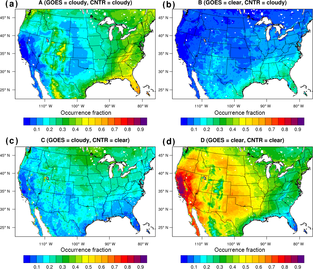
Figure 1Spatial distribution of each contingency category (see Table 2) between the WRF-generated clouds (CNTR simulation) and SatCORPS GOES retrievals averaged over the whole study period.
2.2 WRF-Chem model simulations
The present study employs the WRF-Chem model version 3.6.1. with the updated photolysis scheme. A single domain is used with a horizontal grid size of 12 km (Fig. 1). The meteorological initial and boundary conditions are provided by the NCEP FNL (Final) Operational Global Analysis data with a horizontal resolution of 1∘, which are available every 6 h. The model is initialized at 00:00 UTC on 1 June 2013 and spun up for the first 10 days in the control simulation (CNTR simulation). The meteorological fields are re-initialized every 48 h at 06:00 UTC of a given day to avoid the growth of model errors, and the model is run for 54 h. Here, the first 6 h are allowed for spin-up and discarded in each run. The model outputs for the period of 12:00 UTC on 11 June 2013 through 12:00 UTC on 1 October 2013 are used for the analysis. As the goal of the study is to use and evaluate the modeled clouds and their impact on O3 predictions, nudging is not used. This is different from many previous air quality studies that nudged the meteorology and evaluated modeled O3 with observations. The physics options used are the Morrison two-moment scheme (Morrison et al., 2009) for the microphysics, RRTMG scheme for longwave and shortwave radiation (Iacono et al., 2008), MYNN 2.5 level turbulent kinetic energy (TKE) scheme for the boundary layer parameterization (Nakanishi and Niino, 2006), MYNN surface layer scheme, Noah land surface model (Chen and Dudhia, 2001), and Grell 3-D ensemble scheme (Grell and Devenyi, 2002) for cumulus parameterization with radiation feedback. The initial and boundary conditions for chemical species are obtained from the Model for Ozone and Related Chemical Tracers (MOZART) global simulation of trace gases and aerosols. For each 2-day simulation, the chemical state of the atmosphere at 06:00 UTC is obtained from that at 06:00 UTC of the previous simulation. The MOZART-4 mechanism is used for gas-phase chemistry as described in Knote et al. (2014), and the Model for Simulating Aerosol Interaction and Chemistry (MOSAIC) aerosol module with four bins is used for the aerosol chemistry. Anthropogenic gas and aerosol emissions are adopted from the AQMEII project in which the emissions were projected to 2010 from the NEI 2008 inventory (Campbell et al., 2015). Since Travis et al. (2016) reported that NEI NOx emissions are too high, we reduced NOx emission from all anthropogenic sources by 40 % based on their analysis. Note that the NOx and PAN from the lateral boundaries are also reduced by 40 % in our study. Biomass burning emissions are taken from the Fire Inventory from NCAR (FINN) (Wiedinmyer et al., 2011). Model of Emissions of Gases and Aerosols from Nature (MEGAN) (Guenther et al., 2006) version 2.04 is used for BVOC emissions. As performed in Travis et al. (2016) to better match isoprene flux observations during the Studies of Emissions and Atmospheric Composition, Clouds and Climate Coupling by Regional Surveys (SEAC4RS) field campaign (Toon et al., 2016), we reduced MEGAN isoprene emissions by 15 % over the southeastern US. The photolysis rate calculations utilize the newly implemented the tropospheric ultraviolet and visible (TUV) option in the WRF-Chem model (Hodzic et al., 2018). This new TUV option uses the updated cross section and quantum yield data based on the latest stand-alone TUV model version 5.3 and considers 156 wavelength bins with the resolutions of 1–5 nm. The COD is calculated based on the parameterization given in Chang et al. (1987), which uses cloud liquid water and/or ice water contents and effective droplet radius (assumed to be 10 µm both for liquid and ice droplets). To represent subgrid cloud overlaps, a simple equation of Briegleb (1992) is used, i.e., the effective COD = COD0 × (cloud fraction)1.5, where COD0 is the COD that is calculated following Chang et al. (1987), and the cloud fraction is determined based on the relative humidity in a given grid box. According to Briegleb (1992), applying a power of 1.5 to the cloud fraction is equivalent to the maximum random overlap.
In the present study, we performed two sets of simulations that use WRF-generated clouds in the CNTR simulation and the GOES clouds in the GOES simulation. The GOES simulations were conducted from 06:00 UTC on 11 June 2013 through 12:00 UTC on 1 October 2013. The initial chemistry conditions in the GOES simulation are adopted from the outputs of the CNTR simulation at 06:00 UTC on 11 June 2013. The satellite cloud retrievals are used only to correct photolysis rate and photosynthetically active radiation (PAR) calculations (i.e., only within the TUV model in WRF-Chem). That is, the satellite cloud information is not linked to dynamics, microphysics, and atmospheric radiation. The value of COD is linearly distributed through vertical grids from the cloud bottom to the cloud top within the TUV model as carried out in Ryu et al. (2017). This method is different from the one used in Pour-Biazar et al. (2007) and Tang et al. (2015) in which cloud bottom height used in their photolysis rate calculations is estimated from the meteorological model rather than retrieved from the satellite. The use of model estimates can lead to additional uncertainties in the case of misplaced model clouds compared to observations.
In the present study, PAR calculated from the TUV model is used for the BVOC emissions in MEGAN for all simulations. This is different from the PAR conventionally used in MEGAN, which is simply converted or scaled from the downward shortwave radiation from the atmospheric radiation scheme. In the CNTR (GOES) simulation, the WRF-generated clouds (GOES clouds) are used for the PAR calculation within the TUV model.
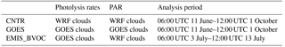
To examine the impact of changes in BVOC emissions on surface O3, another set of sensitivity simulations (EMIS_BVOC simulation) is performed for 10 days (3–12 July 2013), which uses WRF-generated clouds for the PAR calculation and BVOC emissions as in the CNTR simulation but uses the GOES clouds for photolysis rate calculations as in the GOES simulation. The description of the control and sensitivity simulations is summarized in Table 1.
2.3 Observational data
2.3.1 Aircraft data from field campaigns
We evaluate the model performance using airborne measurements made during two field campaigns in 2013, i.e., the NOMADSS (Nitrogen, Oxidants, Mercury and Aerosol Distributions, Sources and Sinks) and the SEAC4RS campaigns. The detailed description of the instrument and measurement data is given in Ryu et al. (2017). The NOMADSS campaign was conducted during 1 June–15 July 2013 mainly over the southeastern US. We use 16 flight-day data at 1 min time intervals for the analysis. Data with solar zenith angles larger than 85∘ are not used. The fire plume data are filtered out by excluding the data showing NO2 (>0.1 ppb) or CO (>120 ppb) aloft at the 4–7 km level. Based on the GOES cloud data, 68 % of flight data are characterized by clear skies and the remaining data (32 %) had clouds in the vertical column where the airplane was located. The SEAC4RS campaign also targeted the southeastern US although the airplane sometimes flew over a larger region including California and the Midwestern US. The period used for the analysis is from 6 August through 23 September 2013, which includes 21 flight days. The time intervals are also 1 min and the data with large solar zenith angles (>85∘) and fire plumes are filtered out. The fraction of data with clouds is 41 % for SEAC4RS. It is noteworthy that SEAC4RS measurements include large and thick clouds in some cases as a few of the campaign goals are to identify the role of deep convection in redistributing pollutants and aerosol–cloud feedbacks, whereas the clouds during NOMADSS were mostly broken clouds.
2.3.2 Ground ozone data
The United States Environmental Protection Agency (EPA) hourly O3 measurements are used for the analysis. To examine the sensitivity of O3 to COD in different chemical regimes, the VOC- and NOx-limited regimes are identified using the ratio of ΔO3 ∕ ΔNOy, following Sillman and He (2002). They reported that the NOx–VOC transition occurs when ΔO3 ∕ ΔNOy = 4–6. Thus, an EPA site is denoted as a VOC-limited (NOx-limited) regime when the ratio is less than 4 (greater than 6). Examples showing the ratio of ΔO3 ∕ ΔNOy for several sites are given in the Supplement (Fig. S1). Among 1299 EPA sites, 1062 are used for the analysis: 24 % of the sites are in the VOC-limited and 76 % in NOx-limited regimes. The remaining 237 sites are not used in the present study because those sites fall into the transitional zone, i.e., ΔO3 ∕ ΔNOy = 4–6. Note that modeled O3 and NOy in the CNTR simulation are used to determine whether an EPA site is in the VOC-limited or NOx-limited regime because NOy measurements are available for limited sites.
Table 2Contingency table for WRF simulation and GOES satellite clouds. The number of data for each category is normalized by the total number of data.
The model bias in the cloud spatial coverage is evaluated using a 2 × 2 contingency table (Table 2), where A and D correspond to hit and correct negative events, respectively, and B and C to false alarm and miss events, respectively. Here, a threshold of 0.3 in hourly COD is used to distinguish between clear and cloudy sky as the lowest detection limit of satellite-retrieved COD over land is estimated at 0.25 in Rossow and Schiffer (1999), and the use of 0.3 poses slightly stricter conditions for cloudiness. The agreement index, which is defined as A+D (WRF correctly predicts cloudy or clear skies), is 69.7 % and the probability of detection (POD) for clouds, A/(A + C), is 55.6 %. It is found that the fraction of errors in missing clouds (C, 19.8 %) is larger than that of predicting clouds that are not present in reality (B, 10.4 %). The overall bias, (A + B)/(A + C), is 0.789 and this means that the WRF underestimates the frequency of cloudy skies. Figure 1 shows the spatial distribution of each contingency category over the CONUS averaged over the whole study period. In general, the eastern US shows higher cloud frequencies than the western US except for parts of the Rocky Mountains and the Pacific Northwest. The largest agreement index appears in central California where the sky condition is mostly clear (Fig. 1d). In terms of errors, the missing cloud rate has its highest frequency (20−35 %) in the Midwestern and northwestern US, while the highest frequency of false alarm (20–30 %) occurs over the southeastern US and southeastern Texas. The sum of categories B and C can be found in Fig. S2. It should be noted that the contingency categories are based on binary results of clear sky or cloudy sky and so they do not provide quantitative comparison of cloud optical properties, e.g., COD. For example, even though the WRF model produces clouds in the right locations (category A), the WRF CODs can differ from those retrieved from satellite data.
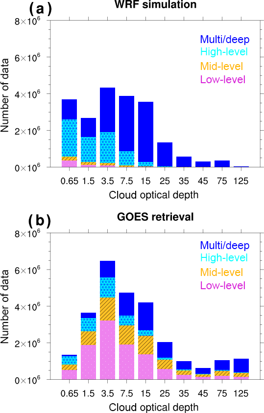
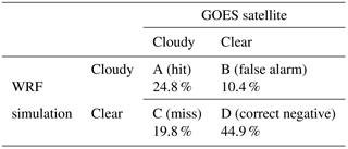
Figure 2Histogram of hourly cloud optical depth (COD) during the daytime (16:00–23:00 UTC) over the CONUS (land only) from the (a) WRF simulation (with the Morrison microphysics and the Grell 3-D schemes) and (b) GOES satellite retrievals. CODs on the x axis represent the mean values of the bins that are 0.3–1, 1–2, 2–5, 5–10, 10–20, 20–30, 30–40, 40–50, 50–100, and 100–150. For a fair comparison, the multilayered WRF clouds are not resolved into cloud layers as this layering cannot be resolved by the satellite.
Figure 2 quantitatively evaluates COD and vertical extent of clouds between the model and satellite retrievals. The vertical extent of clouds is classified based on the International Satellite Cloud Climatology Project (ISCCP) definitions (Rossow and Schiffer, 1999), which are as follows: (i) low-level: cloud top height ≤ 3 km; (ii) mid-level: 3 km < cloud top height ≤ 6 km; (iii) high-level: cloud bottom height > 6 km; and (iv) multilayered or deep convection: cloud bottom height ≤ 6 km and cloud top height > 6 km. Even though multiple cloud layers can be resolved in the WRF model, these kinds of clouds are not resolved in the satellite retrievals used in this study. Thus, for a fair comparison, the multilayered clouds in the WRF model are not further resolved into cloud layers. Note that the liquid and ice water contents from cumulus clouds (parameterized clouds) are included in the model COD calculations.
The frequency distribution of CODs does not have the same shape in the model and observations. The WRF model overpredicts very thin clouds with COD < 1 by a factor of 2, whereas the GOES retrievals show that the most abundant clouds have CODs of 2–5. The majority of optically very thin clouds from the WRF model correspond to high-level cirrus clouds. This is consistent with the result of Cintineo et al. (2013), showing that the Morrison microphysics scheme produces too many upper-level clouds by comparing GOES infrared brightness temperature with the WRF model. Note that the optically-thin multilayered clouds very likely contain cirrus clouds because their top height is greater than 6 km. The WRF model produces fewer clouds with COD > 1 than observed, and the discrepancy is most apparent for optically very thick clouds (COD > 50). As a result, the model COD mean and standard deviation are smaller than those for the retrievals, which are 8.3 and 12.7, respectively, for the WRF model, and 17.8 and 30.8, respectively, for the GOES retrievals.
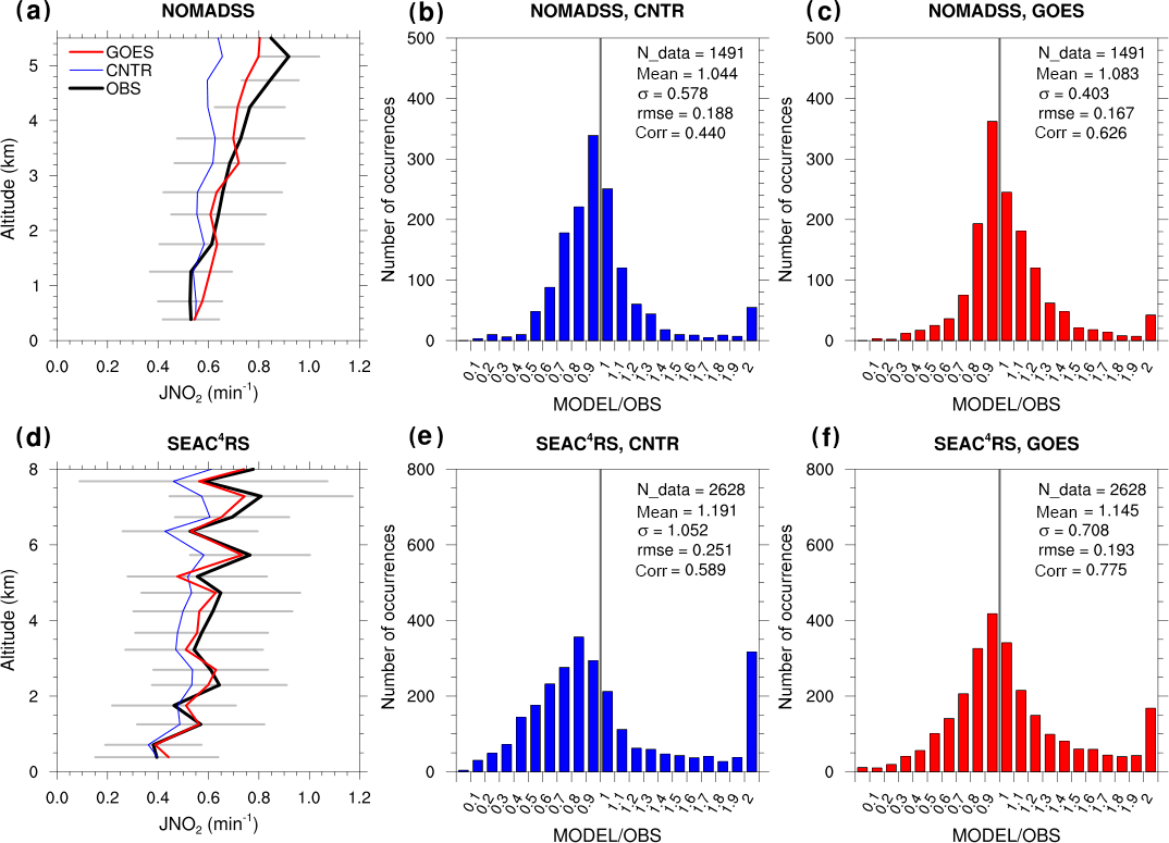
Figure 3Model evaluation with 16 NOMADSS flights (top row) and with 21 SEAC4RS flights (bottom row). Note that only cloudy skies are considered. The comparison is performed for the averaged vertical profiles of JNO2 for (a) NOMADSS and (d) SEAC4RS. The gray horizontal lines indicate the standard deviations from the observations. Histogram of the ratio of JNO2 simulated by the model to JNO2 observed (b) in the CNTR simulation and (c) in the GOES simulation for NOMADSS. Panels (e) and (f) are the same as (b) and (c), respectively, but for SEAC4RS.
Figure 3 compares the cloudy-sky-averaged vertical profiles of NO2 photolysis rates (JNO2) predicted by WRF-Chem and measured during the NOMADSS (Fig. 3a) and SEAC4RS (Fig. 3d) campaigns. The histograms of the ratio of simulated JNO2 to that observed under cloudy conditions are also shown for the CNTR and GOES simulations.
For both campaigns, the simulations with satellite clouds (GOES simulations) generally show better agreement with the observed JNO2 profiles than the CNTR simulations, especially above the boundary layer (above ∼ 2 km). The histograms of the ratio of model JNO2 to observed JNO2 also generally show a better performance in the GOES simulation than in the CNTR simulation: the mean of the ratio is closer to 1 in the GOES simulation than in the CNTR simulation for SEAC4RS, the standard deviations are reduced in the GOES simulation compared to those in the CNTR simulation for both campaigns, the root-mean-square errors are lowered in the GOES simulation compared to those in the CNTR simulation, and the correlation coefficients are closer to 1 in the GOES simulation than in the CNTR simulation. For NOMADSS, the large bias in the highest ratio bin (> 2) is 24 % less in the GOES simulation than in the CNTR simulation. The reduction of the large bias (bin > 2) in the GOES simulation is more substantial for SEAC4RS and reaches 47 %. These reductions are attributed to a better representation of the below-cloud and inside-cloud conditions when satellite clouds are used (not shown). This is because the number of data influenced by thick clouds is larger in SEAC4RS than in NOMADSS and the measurements in the presence of those thick clouds were mostly made under below-cloud or inside-cloud conditions.
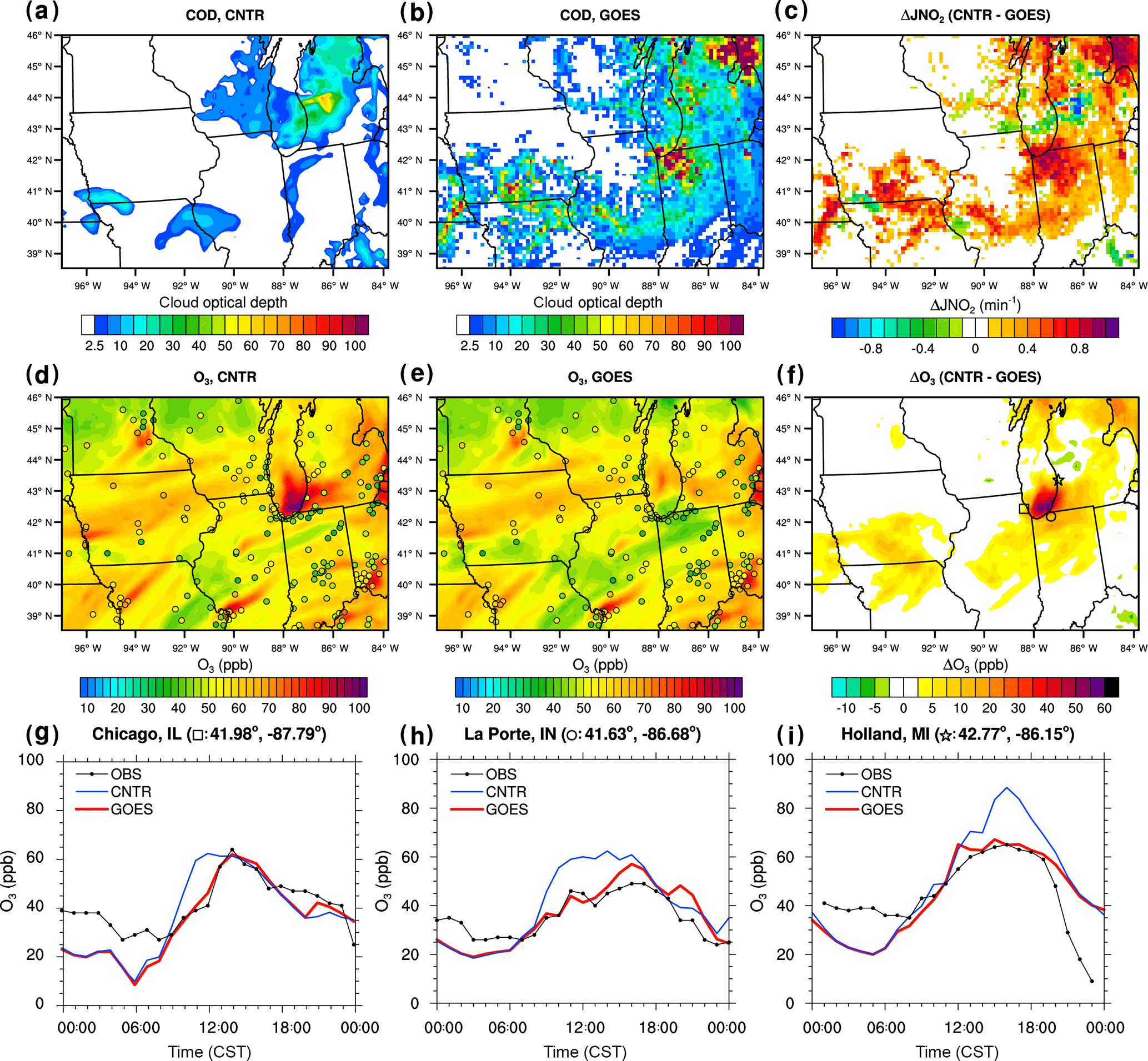
Figure 4Horizontal distributions of cloud optical depth at 13:00 CST (= 19:00 UTC) on 8 July 2013 (a) in the CNTR simulation and (b) in the GOES simulation. Horizontal distributions of O3 at 13:00 CST on 8 July 2013 at the lowest model level (shaded) (d) in the CNTR simulation and (e) in the GOES simulation. The circles indicate EPA ozone measurements. Panels (c) and (f) show the difference in JNO2 and O3, respectively, between the simulations (i.e., CNTR simulation minus GOES simulation). (g–i) Time series of O3 at the square (Chicago, IL), circle (La Porte, IN), and star (Holland, MI) that are marked in (f), respectively.

Figure 5(a) Spatial distribution of maximum daily 8 h average O3 (MDA8 O3) at the lowest model level averaged over the whole analysis period in the CNTR simulation. (b) Difference in MDA8 O3 at the lowest model level between the control and GOES simulations (i.e., CNTR minus GOES).
5.1 An example on 8 July 2013 in the Midwestern US
Figure 4 shows an example of how model errors in cloud fields impact O3 predictions. This example includes thunderstorm systems over the Midwestern US. The CNTR simulation misses clouds or underpredicts CODs over metropolitan Chicago and the region south of Lake Michigan. This results in the overprediction of JNO2 by up to 0.54 min−1 (∼ 90 %) compared to that computed using GOES clouds. The resulting changes in O3 concentration are regional and the O3 overprediction in the plume originating from the Chicago area is up to 62 ppb (∼ 60 % of O3 in the CNTR simulation). As a result of the cloud corrections, O3 in the GOES simulation agrees better with observations in those regions (compare Fig. 4d with e and g, h, i). The time series of O3 at the three sites (marked in Fig. 4f) near Lake Michigan show particularly improved agreement with observations when satellite clouds are used. The large O3 biases of 20.5 ppb at 11:00 CST at Chicago, IL; 19.2 ppb at 13:00 CST at La Porte, IN; and 23.5 ppb at 16:00 CST at Holland, MI, in the CNTR simulation are reduced to 1.7, 3.2 ppb, and −0.11 ppb in the GOES simulation, respectively. It is also apparent that the bias reduction in O3 shifts eastward (from Chicago, IL, to Holland, MI) as the thunderstorm moves eastward during the day. An important implication of this finding is that errors in cloud predictions can lead to wrong O3 alerts in areas where the model does not predict clouds well. For example, the maximum daily 8 h average O3 (MDA8 O3) concentration is 75.3 ppb at Holland, MI, in the CNTR simulation (Fig. 4i) and this value exceeds the O3 standard (70 ppb for MDA8 O3). However, the MDA8 O3 concentration at the same location is 63.0 ppb in the GOES simulation and 60.4 ppb in the observation. Therefore, an O3 action alert would have been issued if the CNTR simulation results were used, which would result in a false alarm. The example shown here emphasizes the important roles of clouds in the Great Lakes region where large O3 biases have been reported previously in air quality forecasts (e.g., Cleary et al., 2015). The correction of clouds both over the lakes and in the upstream regions (mostly large cities located to the west-southwest of the lakes) significantly reduces the O3 bias. It is also shown that polluted air masses from the source regions can be advected over the lakes (not shown). In this case in which precursor levels can be high over the lakes, the presence of clouds over the lakes can greatly affect O3 formation over the lakes.
In general, the regions exhibiting O3 differences between the two simulations coincide with the regions where JNO2 values are different. More importantly, large O3 differences are found near urban areas (e.g., Chicago, IL; downwind area of Kansas City, MO; Omaha, NE, and its downwind area). Even though the difference in COD or JNO2 is significant in central Indiana, for example, the difference in O3 in the region is relatively small compared to that near Lake Michigan.
5.2 Maximum daily 8 h average O3
Figure 5 shows the maps of MDA8 O3 averaged over the study period for the CNTR simulation and the difference in MDA8 O3 between the CNTR and GOES simulations. The spatial distribution of MDA8 O3 in the GOES simulation is similar to that in the CNTR simulation (thus the GOES spatial average is not shown here), but the O3 levels are considerably different. In Fig. 5b, the Midwestern, eastern, and northwestern US regions show the largest O3 differences, up to 5.8 ppb, with lower O3 levels in the GOES simulation. These regions generally belong to the contingency category C (Midwestern and northwestern US) or category A (eastern US). However, the regions with negative differences, i.e., some places over the south-southeastern US, coincide with the contingency category B. These differences are expected and can be interpreted as follows: when the WRF model misses clouds (clear sky in the CNTR simulation, category C) or underestimates COD (as seen in Fig. 2), surface O3 is overestimated. When the WRF model generates clouds that are not present in reality (clear sky in the satellite retrievals, category B), surface O3 is underestimated. It should be noted that not all regions belonging to category B or C have significant O3 differences. Interestingly, the regions exhibiting significantly large O3 differences coincide with large urban areas, e.g., Seattle, WA; Los Angeles, CA; Chicago, IL; Cleveland, OH; Houston, TX; New Orleans, LA; Atlanta, GA; and Miami, FL. The reasons for this result are explored in Sect. 5.4 and 5.5.
The performance of the GOES simulation is found to be better than that of the CNTR simulation compared to observations: for example, under cloudy conditions (COD > 20; see Sect. 5.4 for the criterion), the root-mean-square error of MDA8 O3 in the GOES (CNTR) simulation is 13.2 ppb (16.9 ppb) and the correlation coefficient of MDA8 O3 in the GOES (CNTR) simulation is 0.5 (0.4).
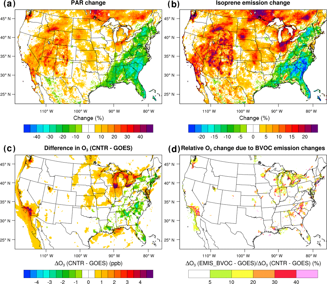
Figure 6Spatial distributions of (a) PAR change and (b) isoprene emission change from biogenic sources between EMIS_BVOC and GOES simulations, (EMIS_BVOC–GOES)/GOES, averaged over the period of 3–12 July 2013. (c) Difference in O3 between the CNTR and GOES simulations. (d) Ratio of O3 difference between EMIS_BVOC and GOES simulations to O3 difference between CNTR and GOES simulations, i.e., ΔO3 (EMIS_BVOC–GOES) ∕ ΔO3 (CNTR–GOES). Note that the grids that have considerable O3 difference between CNTR and GOES simulations (> 1 ppb) are depicted in (d).
5.3 Relative contribution to O3 errors from photolysis rates and BVOC emissions
It is expected that reduced BVOC emissions (especially isoprene) due to the presence of clouds can also decrease O3 formation. Figure 6 shows the spatial distributions of relative changes in PAR and isoprene emission between the EMIS_BVOC and GOES simulations averaged over a 10-day period. Because the WRF model tends to underestimate COD or is not able to reproduce clouds in the Midwestern and western US, PAR and biogenic isoprene emissions are larger in the EMIS_BVOC simulation than in the GOES simulation. However, the model overestimates COD or produces clouds that are not present in reality over the southeastern US; thus PAR and biogenic isoprene emissions are lower in the EMIS_BVOC simulation than in the GOES simulation. The change in PAR (biogenic isoprene emissions) resulting from the difference in cloud fields between the WRF model and satellite retrievals is up to % (±25 %). Figure 6d shows the O3 difference between EMIS_BVOC and GOES simulations relative to the O3 difference between CNTR and GOES simulations (Fig. 6c). It is seen that the contribution of changes in BVOC emissions is considerable only for some regions and it ranges from ∼ 10 to 40%. The average contribution of changes in BVOC emissions over land is ∼ 20 % compared to changes of BVOC emissions plus photolysis rates using GOES satellite clouds. The contribution of BVOC emissions is larger (∼ 40%) in urban areas over the southeast (specifically in Charlotte, NC). The difference in O3 in Charlotte, NC, resulting from changes in BVOC emissions is about 1.5 ppb and that from changes in both photolysis rates and BVOC emissions is about 3.5 ppb. In some regions, such as the Midwest, western Pennsylvania, and central New York, the effect of BVOC emissions is negligible.
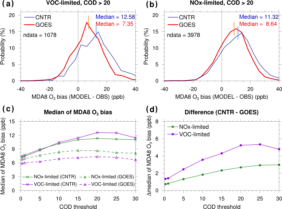
Figure 7(a) Probability density function of maximum daily 8 h average (MDA8) O3 bias (model value minus observation value) for the VOC-limited regime under cloudy-sky conditions defined with a COD threshold of 20. (b) Same as (a), but for the NOx-limited regime. (c) Median values of MDA8 O3 bias with respect to COD threshold in the CNTR simulation (solid lines with cross marks) and in the GOES simulation (dashed line with triangles) for VOC-limited (purple color) and NOx-limited regimes (green color). (d) Difference in median values of MDA8 O3 bias between the two simulations with respect to COD threshold (i.e., CNTR minus GOES).
5.4 Cloud effects on ozone bias in VOC- and NOx-limited regimes
In this section, we examine the effects of clouds on O3 in VOC-limited and NOx-limited regimes in order to understand the reasons for a stronger O3 response to cloud corrections in urban areas than in the remote regions. Figure 7 shows how cloud corrections affect O3 errors in different regimes. Here, MDA8 O3 is used to compute the model O3 bias (simulation minus observation). Figure 7a and b show the probability density functions of the model O3 bias for the CNTR and GOES simulations, respectively, at all ground sites experiencing considerably thick (COD > 20) clouds. In this example, an EPA site is considered under cloudy-sky conditions when hourly COD greater than the chosen threshold (here, 20) is present at the site for at least 4 h within the 8 h time window on a given day. The decrease in the O3 bias for the VOC-limited regime is significant, and the difference in median values between the two simulations is 5.2 ppb. The decrease in O3 bias for NOx-limited regimes (2.7 ppb) is about 2 times smaller than that for the VOC-limited regime. An important result is that the frequency of very large biases (e.g., greater than 20 ppb) is substantially reduced when cloud fields are corrected, especially for the VOC-limited regime. This implies that more accurate cloud predictions ultimately improve the accuracy of O3 alert predictions, especially in polluted urban areas.
Figure 7c shows the change in median values of MDA8 O3 bias for a range of COD thresholds. We find that the O3 bias increases with increasing cloudiness in the CNTR simulation. As previously mentioned, the O3 bias is generally larger for VOC-limited regimes than for NOx-limited regimes. When the radiation fields are corrected with satellite clouds, the model O3 bias is considerably reduced (but not zero). In addition, the O3 bias in the GOES simulation does not increase as much as that in the CNTR simulation when cloudiness increases. This implies that there are other sources of O3 biases in the GOES simulation, which are not likely associated with cloudiness. The other error sources can be precursor emissions, mixing or transport, and deposition. Figure 7d compares the median values of MDA8 O3 bias between the two simulations (CNTR minus GOES) and shows that the difference in MDA8 O3 between the two simulations clearly increases as the COD threshold increases and that the effect of cloud correction is larger in VOC-limited than in NOx-limited regimes. The reduced O3 bias as a result of cloud corrections ranges from 1 to 5 ppb depending on CODs and chemistry regimes. This represents up to ∼ 40 % of the total O3 bias under cloudy conditions in the current model version (e.g., 5.2 of 12.6 ppb for COD threshold of 20 in VOC-limited regimes). Note that the results for the sites in the transitional zone (the slope of ΔO3 ∕ ΔNOy is 4–6) showed that the effects of cloud in the transitional zone are intermediate, that is, larger than those for NOx-limited regimes but smaller than those for VOC-limited regimes (not shown).
We performed additional analysis by dividing VOC- and NOx-limited sites into groups that have similar ranges of peak MDA8 O3 concentration during the period of June–September 2013 (Fig. S3). All sites are grouped into bins with a peak value of MDA8 O3 ranging from larger than 75, 70–75, 65–70, 60–65 ppb, to smaller than 60 ppb. The maximum reduction in O3 bias due to cloud corrections is obtained for the VOC-limited sites with a peak MDA8 O3 of 65–70 ppb and reaches ∼ 8 ppb. The maximum reduction for NOx-limited sites, however, is ∼ 4 ppb and found for the sites with a peak MDA8 O3 of 70–75 ppb. Although the degree of the O3 bias reduction varies somewhat among the bins for a given ozone regime, the effects of cloud correction on O3 bias reduction remain larger in VOC-limited regimes than NOx-limited regimes.
We examine the O3 bias over the southeastern US where large overpredictions at the surface have been reported (e.g., Travis et al., 2016) in the Supplement. It is found that a considerable portion of O3 bias is attributable to inaccurate cloud predictions over the southeastern US, but the degree of the effects of clouds is smaller than that over the CONUS as a whole (Fig. S4). The maximum reduction in O3 bias due to inaccurate cloud predictions is 4.5 ppb over the southeastern US and 5.3 ppb over the CONUS. Still, large O3 biases of ∼ 11 ppb are present over the southeastern US (compared to those of 6–9 ppb over the CONUS) even though the clouds and radiation fields that are relevant to photochemistry are corrected. This result implies that errors resulting from other processes exist and are responsible for the surface O3 overpredictions over the southeastern US. More in-depth studies that find and quantify errors are therefore required to better predict the O3 over the southeastern US as well as CONUS.
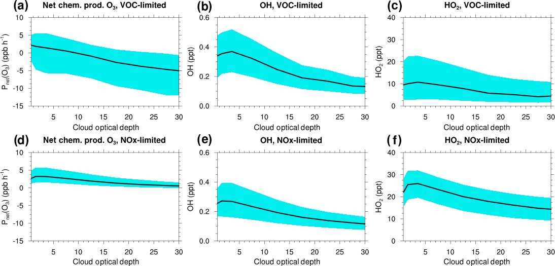
Figure 8(a) Net chemical production of O3, (b) OH concentration, and (c) HO2 concentration with variations of cloud optical depth for the VOC-limited regime. The black line indicates the median, and cyan shading indicates the 25th and 75th percentiles. Similar variables are shown for the NOx-limited regimes (d–f).
Table 3Sensitivity coefficient of O3 to JNO2, i.e., dln(O3) ∕ dln(JNO2). The values of dln(O3) ∕ dln(JNO2) for the period of 09:00–13:00 LST are averages over only the CONUS EPA stations that have monotonically increasing O3 concentrations with time.
5.5 Ozone formation sensitivity to changes in photolysis rates
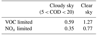
The difference in O3 sensitivity to changes in photolysis rates (resulting from the presence of clouds) in different regimes is determined by calculating dln(O3) ∕ dln(JNO2) ratios as in Kleinman (1991). Table 3 lists those sensitivity coefficients of O3 to JNO2 and shows that O3 is more sensitive to JNO2 in VOC-limited than in NOx-limited regimes, being 1.69 times larger under cloudy-sky conditions and 1.65 times greater under clear-sky conditions. Similar sensitivities were reported for OH by Berresheim et al. (2003) with the sensitivity of OH to JO1D, dln(OH) ∕ dln(JO1D), of 0.8 at high NO2 levels (∼ 10 ppb) and 0.68 at low to moderate NO2 levels (∼ 1 ppb). The corresponding sensitivities from our study are 1.1 for VOC-limited regimes and 0.66 for NOx-limited regimes under clear-sky conditions. Similar results are also found for the net chemical production of O3 and OH concentration, revealing stronger responses to changes in cloudiness in VOC-limited regimes than NOx-limited regimes (Fig. 8). It is interesting to note that OH and HO2 have local maxima at CODs between 2 and 5. As shown in Ryu et al. (2017), the enhancement of actinic flux at the surface due to optically thin clouds (CODs < 5) is considerable for high-level clouds, i.e., cirrus. The local maxima, therefore, likely result from the fact that the GOES clouds have the largest portion of cirrus for CODs of 2–5 as seen in Fig. 2b. Figure 8 also shows that the variation (defined by 25 and 75 percentiles) of net chemical production of O3 with respect to COD is much larger in VOC-limited conditions. This result suggests that predicting O3 under cloudy conditions is likely more difficult in VOC-limited than in NOx-limited regimes. It is also noticeable that the HO2 radical concentration remains relatively high in NOx-limited regimes even under cloudy conditions compared to the VOC-limited regimes. Note that the results of WRF-Chem here include the effect of both photolysis rates and BVOC emissions.
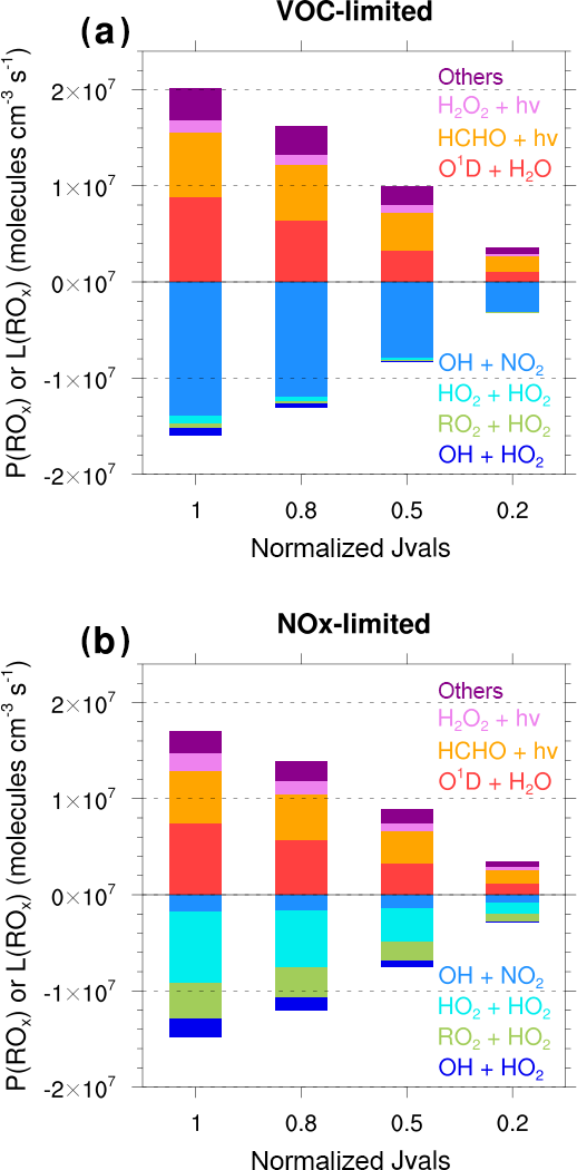
Figure 9Results of box modeling for production and loss rates of ROx (= OH + HO2 + RO2) radicals. “Others” in the legend indicates the photolysis of VOCs and reactions between alkenes and O3. The value of 1 of normalized Jvals on the x axis indicates the photolysis rates for clear-sky conditions.
A simplified box model (BOXMOX; Knote et al., 2015) simulation using the same chemical mechanism (MOZART-4) as in WRF-Chem was performed to better understand O3 sensitivity to changing cloudiness in different chemistry regimes. The emission rates for the VOC-limited (NOx-limited) regime are those of the Chicago urban (rural) area in the WRF-Chem simulation. The initial conditions are taken from the CNTR simulation at 09:00 CST on 7 July 2013 in the Chicago suburban area for both regimes. Dry deposition is not considered. Photolysis rates for all species that are photodissociable are varied from clear- to cloudy-sky conditions with up to 80 % reduction. The 80 % reduction roughly corresponds to COD of 35 (not shown). The box model is integrated for 3 h and photolysis rates are kept constant during the simulation (i.e., no diurnal variations). The box model results are found to be consistent with the results from the WRF-Chem simulations: the variations of O3 and OH with respect to decreasing photolysis rates are larger in the VOC-limited regime than in the NOx-limited regime (Fig. S5). Note that the net chemical production of O3 obtained from the box model results also shows a larger sensitivity to cloudiness in VOC-limited regimes than in NOx-limited regimes, which is similar to Fig. 8a and d (not shown). Figure 9 shows production and loss terms of ROx (= OH + HO2 + RO2) radicals with variations in photolysis rates for VOC-limited and NOx-limited regimes. In both regimes, the decreased sunlight due to clouds reduces OH formation by photodissociation of O3 (primary source of OH). The larger sensitivity of OH radicals to COD in VOC-limited regimes as seen in Fig. 8 is associated with the loss of OH by the radical termination reaction between OH and NO2 under NOx-rich conditions, which leads to the large decrease in OH (Fig. 9a). However, in NOx-limited regimes, the radical termination reactions are the radical–radical reactions (Fig. 9b). In this regime, OH mainly reacts with VOCs and propagates through radical cycles by producing HO2 ∕ RO2 radicals, rather than being terminated by the reaction with NO2. Given that the reaction between NO and HO2 becomes the largest source of OH budget (secondary source of OH) at an NOx concentration of ∼ 1 ppb (Ehhalt and Rohrer, 2000; Eisele et al., 1997), OH can be relatively less sensitive to the changes in radiation. Note that the mean daytime NOx concentration over the CONUS in NOx-limited regimes it is 1.2 ppb and that in VOC-limited regimes is 6.7 ppb for this study period. Another attribute is a greater contribution of H2O2 photodissociation to the production of ROx in NOx-limited regimes than that of HNO3, which is negligible. Unlike the radical terminated in VOC-limited conditions, a non-negligible amount of terminated radicals can be recycled in the NOx-limited regime.
It should be emphasized that our study was performed using a specific representation of the cloud microphysics by Morrison et al. (2009) and cumulus parameterization (Grell and Devenyi, 2002). To test the robustness of our results with regard to the representation of clouds, another microphysics scheme, the Thompson scheme (Thompson et al., 2008), is employed for a 10-day (3 July–12 July 2013) sensitivity simulation. The COD comparison in Fig. S6 shows that with the Thompson scheme the model predicts fewer clouds for all ranges of CODs compared to GOES retrievals, except for the very thin ones (COD < 1) in which the number of those clouds is still overpredicted as seen in the simulation with the Morrison scheme. Compared to the Morrison scheme, the Thompson scheme produces significantly less high-level (cirrus) clouds. This is also consistent with the findings of Cintineo et al. (2013). Despite this difference, the shape of the COD distribution from the two microphysics schemes is rather similar.
The MDA8 O3 bias with the Thompson scheme is evaluated (Fig. S7) and compared to that of the Morrison scheme for the same period. Under the conditions of COD greater than 20, for example, the baseline simulation with the Thompson scheme (that uses model-generated clouds) shows that a median bias (14.79 ppb) is a bit smaller than that with the Morrison scheme (16.22 ppb) for that period in VOC-limited regimes. In the sensitivity simulation with the Thompson scheme that uses GOES satellite clouds for photochemistry, the median bias is reduced by 5.45 ppb (∼ 37%, Fig. S7a) in VOC-limited regimes and by 2.06 ppb (∼ 20%, Fig. S7c) in NOx-limited regimes, which is consistent with the results of our base simulation. The degree of the effects of cloud correction in the sensitivity simulations with the Thompson scheme, ranging from 0.5 to 5.5 ppb, is similar to that found in our base simulation with the Morrison scheme. Therefore, the general conclusions remain the same: i.e., errors in O3 predictions resulting from errors in cloud predictions are considerable (up to ∼ 5 ppb on average) and the effects of cloud corrections are larger in VOC-limited regimes than in NOx-limited regimes.
To estimate the sensitivity of our results to cumulus parameterization schemes, sensitivity simulations with the Grell–Freitas scheme (Grell and Freitas, 2014) are performed. As performed for the microphysics scheme, a period of 10 days (3–12 July 2013) was considered. In Fig. S8, the histograms of CODs obtained for the 10-day period from the Grell–Freitas scheme and from the Grell 3-D scheme show that the distributions of CODs are in general similar to each other. The Grell–Freitas scheme tends to produce fewer clouds with small or moderate CODs (Fig. S8). As shown in Fig. S9, the degree of cloud correction in reducing O3 bias is larger in VOC-limited regimes than in NOx-limited regimes in the simulation with the Grell–Freitas scheme, and thus the conclusions originally drawn remain unchanged.
We performed quantitative analyses of the WRF-Chem model mesoscale (12 km) simulations to determine how much errors in cloud predictions contribute to errors in surface O3 predictions during summertime over the CONUS. Clouds were generated using the Morrison microphysics and Grell 3-D cumulus parameterization schemes. It is found that the WRF-Chem model is able to generate roughly 55 % of the clouds in the right locations by comparing to satellite clouds. A quantitative comparison of COD shows that the WRF-Chem model predicts too many thin cirrus clouds with CODs less than 1, and also considerably underpredicts the optical depths for the majority of cloud systems.
The errors in cloud predictions can lead to large hourly O3 biases of up to 60 ppb, for example, for specific cases in which the model misses deep convective clouds that are present in reality. On average, the errors in MDA8 O3 of 1–5 ppb are found to be attributable to errors in cloud predictions under cloudy-sky conditions. We separately quantify the contribution of changes in photolysis rates and emissions of light-dependent BVOCs to cloud-related errors in surface O3. The contribution of photolysis rates to surface O3 is larger (∼ 80 % on average) than that of BVOC emissions. The contribution of BVOC emissions to O3 can become important (∼ 40 %) in the VOC-limited regimes in which BVOC emissions are large (i.e., cities of the southeastern US).
The effects of cloud corrections are more impactful in VOC-limited (or high-NOx) than in NOx-limited (or low-NOx) regimes. The sensitivity of O3 with respect to COD is about 2 times larger in VOC-limited than in NOx-limited regimes. This finding is consistent with the box modeling results that were performed for typical urban and rural conditions under varying photolysis rates. The production of radicals (OH, HO2, and RO2) decreases with decreasing photolysis rates in the presence of clouds. The primary reason for the larger sensitivity of O3 formation to clouds in VOC-limited regimes is that the loss of OH is much stronger in VOC-limited regimes due to the reaction with NO2. Thus, OH cannot readily propagate through the radical cycles. In NOx-limited regimes, the radicals terminated from the radical cycles are mostly HO2 and RO2 rather than OH. Thus, OH can remain in the cycles and continue to produce HO2 and RO2 by reacting with VOCs before termination. The interconversion of HO2 to OH is the dominant process in NOx-limited regimes, and therefore OH and O3 formations are less sensitive to changes in radiation.
We showed that considerable reduction in O3 bias is achieved by correcting cloud-related radiation fields; however, O3 is still overpredicted by the WRF-Chem model. The remaining bias likely results from other processes involved in the O3 life cycle such as precursor emissions from both anthropogenic and biogenic sources, transport, turbulent mixing, and dry deposition, for which quantitative assessment is beyond the scope of this study.
One should keep in mind that the quantitative estimate of the O3 bias related to the cloud effects on radiation as reported in this study could be sensitive to several factors. In particular, this study is based on a particular configuration of the WRF-Chem model with regard to the radiation, microphysics, cumulus, boundary layer parameterization, and the chemistry scheme. We have tested the sensitivity of our results to the choice of microphysics and cumulus parameterization schemes, and have shown that MDA8 O3 biases are reduced by up to ∼ 5 ppb with the satellite cloud corrections in the simulations with the different microphysics and cumulus parameterization schemes, which is consistent with the results found in our base simulations.
This study suggests that accurate cloud predictions through data assimilation or cloud mask corrections with near-real-time satellite cloud data would improve the accuracy of O3 predictions and that the benefit is expected to be greater in VOC-limited than in NOx-limited regimes. It should be noted that our estimates are based on WRF-Chem simulations that use initial and boundary conditions from meteorological reanalysis data, which is an improved estimate of the meteorological state compared to forecast data, and thus the reduction of errors in O3 predictions could be even greater in a forecasting setting. From the perspective of the O3 forecast, our study indicates that there is a need for an enhanced understanding of the evolution of errors in O3 forecasts associated with errors in cloud forecasts, and for optimizing the use of meteorological forecasts to allow more accurate near-term O3 predictions. The present study corrects cloud fields in WRF using only satellite clouds for radiation that is relevant to photochemistry, and those cloud corrections do not affect other meteorological variables such as surface temperature, wind, humidity, boundary layer height, etc. In a future study, we plan to examine the effects of satellite cloud assimilation on near-term O3 forecasts using enhanced forecasts such as the Rapid Refresh products from NOAA (Benjamin et al., 2016) that take into account cloud data assimilation to derive meteorology. Rapid Refresh uses satellite cloud products as well as cloud observations from the ground and considers the thermodynamic balance between temperature and humidity due to the presence of clouds. Thus, this will allow the investigation of the effects of cloud assimilation on O3 forecasts not only through changes in radiation for photochemistry but also through changes in meteorological variables.
The air borne measurement data for SEAC4RS are available at https://www-air.larc.nasa.gov/cgi-bin/ArcView/seac4rs, and those for NOMADSS are available at http://data.eol.ucar.edu/master_list/?project=SAS. The model codes and simulation data used in this study can be obtained from the authors upon request. The GOES cloud retrievals are available at https://satcorps.larc.nasa.gov or can be found in https://search.earthdata.nasa.gov/ with keywords of CER_GEO_Ed4_GOE13_NH_V01 for GOES13 and CER_GEO_Ed4_GOE15_NH_V01 for GOES15. The EPA ozone data can be downloaded at https://aqs.epa.gov/aqsweb/airdata/download_files.html#Raw.
The supplement related to this article is available online at: https://doi.org/10.5194/acp-18-7509-2018-supplement.
The authors declare that they have no conflict of interest.
We acknowledge Samuel Hall and Kirk Ullmann for providing actinic flux data
that are used for supplementary analysis and George Grell and Geoff Tyndall for
helpful discussions. This study is supported by NASA-ROSES grant
NNX15AE38G. Patrick Minnis was supported by the NASA Modeling, Analysis, and
Prediction Program. The National Center for Atmospheric Research is
sponsored by the National Science Foundation. We would like to acknowledge
high-performance computing support from Cheyenne (https://doi.org/10.5065/D6RX99HX)
provided by NCAR's Computational and Information Systems Laboratory,
sponsored by the National Science Foundation.
Edited by: Bryan N. Duncan
Reviewed by: three anonymous referees
Bei, N., Lei, W., Zavala, M., and Molina, L. T.: Ozone predictabilities due to meteorological uncertainties in the Mexico City basin using ensemble forecasts, Atmos. Chem. Phys., 10, 6295–6309, https://doi.org/10.5194/acp-10-6295-2010, 2010.
Benjamin, S. G., Weygandt, S. S., Brown, J. M., Hu, M., Alexander, C. R., Smirnova, T. G., Olson, J. B., James, E. P., Dowell, D. C., Grell, G. A., Lin, H., Peckham, S. E., Smith, T. L., Moninger, W. R., Kenyon, J. S., and Manikin, G. S.: A North American Hourly Assimilation and Model Forecast Cycle: The Rapid Refresh, Mon. Weather Rev., 144, 1669–1694, https://doi.org/10.1175/MWR-D-15-0242.1, 2015.
Berresheim, H., Plass-Dülmer, C., Elste, T., Mihalopoulos, N., and Rohrer, F.: OH in the coastal boundary layer of Crete during MINOS: Measurements and relationship with ozone photolysis, Atmos. Chem. Phys., 3, 639–649, https://doi.org/10.5194/acp-3-639-2003, 2003.
Briegleb, B. P.: Delta-Eddington approximation for solar radiation in the NCAR community climate model, J. Geophys. Res.-Atmos., 97, 7603–7612, https://doi.org/10.1029/92JD00291, 1992.
Brioude, J., Angevine, W. M., Ahmadov, R., Kim, S.-W., Evan, S., McKeen, S. A., Hsie, E.-Y., Frost, G. J., Neuman, J. A., Pollack, I. B., Peischl, J., Ryerson, T. B., Holloway, J., Brown, S. S., Nowak, J. B., Roberts, J. M., Wofsy, S. C., Santoni, G. W., Oda, T., and Trainer, M.: Top-down estimate of surface flux in the Los Angeles Basin using a mesoscale inverse modeling technique: assessing anthropogenic emissions of CO, NOx and CO2 and their impacts, Atmos. Chem. Phys., 13, 3661–3677, https://doi.org/10.5194/acp-13-3661-2013, 2013.
Brown-Steiner, B., Hess, P. G., and Lin, M. Y.: On the capabilities and limitations of GCCM simulations of summertime regional air quality: A diagnostic analysis of ozone and temperature simulations in the US using CESM CAM-Chem, Atmos. Environ., 101, 134–148, https://doi.org/10.1016/j.atmosenv.2014.11.001, 2015.
Campbell, P., Zhang, Y., Yahya, K., Wang, K., Hogrefe, C., Pouliot, G., Knote, C., Hodzic, A., San Jose, R., Perez, J. L., Jimenez Guerrero, P., Baro, R., and Makar, P.: A multi-model assessment for the 2006 and 2010 simulations under the Air Quality Model Evaluation International Initiative (AQMEII) phase 2 over North America: Part I. Indicators of the sensitivity of O3 and PM2.5 formation regimes, Atmos. Environ., 115, 569–586, https://doi.org/10.1016/j.atmosenv.2014.12.026, 2015.
Carter, W. P. L.: Development of the SAPRC-07 chemical mechanism, Atmos. Environ., 44, 5324–5335, https://doi.org/10.1016/j.atmosenv.2010.01.026, 2010.
Chang, J. S., Brost, R. A., Isaksen, I. S. A., Madronich, S., Middleton, P., Stockwell, W. R., and Walcek, C. J.: A three-dimensional Eulerian acid deposition model: Physical concepts and formulation, J. Geophys. Res.-Atmos., 92, 14681–14700, https://doi.org/10.1029/JD092iD12p14681, 1987.
Chen, F. and Dudhia, J.: Coupling an Advanced Land Surface–Hydrology Model with the Penn State–NCAR MM5 Modeling System. Part I: Model Implementation and Sensitivity, Mon. Weather Rev., 129, 569–585, https://doi.org/10.1175/1520-0493(2001)129<0569:CAALSH>2.0.CO;2, 2001.
Cintineo, R., Otkin, J. A., Xue, M., and Kong, F.: Evaluating the Performance of Planetary Boundary Layer and Cloud Microphysical Parameterization Schemes in Convection-Permitting Ensemble Forecasts Using Synthetic GOES-13 Satellite Observations, Mon. Weather Rev., 142, 163–182, https://doi.org/10.1175/MWR-D-13-00143.1, 2013.
Cleary, P. A., Fuhrman, N., Schulz, L., Schafer, J., Fillingham, J., Bootsma, H., McQueen, J., Tang, Y., Langel, T., McKeen, S., Williams, E. J., and Brown, S. S.: Ozone distributions over southern Lake Michigan: comparisons between ferry-based observations, shoreline-based DOAS observations and model forecasts, Atmos. Chem. Phys., 15, 5109–5122, https://doi.org/10.5194/acp-15-5109-2015, 2015.
Dabberdt, W. F., Carroll, M. A., Baumgardner, D., Carmichael, G., Cohen, R., Dye, T., Ellis, J., Grell, G., Grimmond, S., Hanna, S., Irwin, J., Lamb, B., Madronich, S., McQueen, J., Meagher, J., Odman, T., Pleim, J., Schmid, H. P. and Westphal, D. L.: Meteorological Research Needs for Improved Air Quality Forecasting: Report of the 11th Prospectus Development Team of the U.S. Weather Research Program∗, Bull. Am. Meteorol. Soc., 85, 563–586, https://doi.org/10.1175/BAMS-85-4-563, 2004.
Ehhalt, D. H. and Rohrer, F.: Dependence of the OH concentration on solar UV, J. Geophys. Res. Atmospheres, 105, 3565–3571, https://doi.org/10.1029/1999JD901070, 2000.
Eisele, F. L., Mount, G. H., Tanner, D., Jefferson, A., Shetter, R., Harder, J. W., and Williams, E. J.: Understanding the production and interconversion of the hydroxyl radical during the Tropospheric OH Photochemistry Experiment, J. Geophys. Res.-Atmos., 102, 6457–6465, https://doi.org/10.1029/96JD02207, 1997.
Fiore, A. M., Dentener, F. J., Wild, O., Cuvelier, C., Schultz, M. G., Hess, P., Textor, C., Schulz, M., Doherty, R. M., Horowitz, L. W., MacKenzie, I. A., Sanderson, M. G., Shindell, D. T., Stevenson, D. S., Szopa, S., Van Dingenen, R., Zeng, G., Atherton, C., Bergmann, D., Bey, I., Carmichael, G., Collins, W. J., Duncan, B. N., Faluvegi, G., Folberth, G., Gauss, M., Gong, S., Hauglustaine, D., Holloway, T., Isaksen, I. S. A., Jacob, D. J., Jonson, J. E., Kaminski, J. W., Keating, T. J., Lupu, A., Marmer, E., Montanaro, V., Park, R. J., Pitari, G., Pringle, K. J., Pyle, J. A., Schroeder, S., Vivanco, M. G., Wind, P., Wojcik, G., Wu, S., and Zuber, A.: Multimodel estimates of intercontinental source-receptor relationships for ozone pollution, J. Geophys. Res.-Atmos, 114, D04301, https://doi.org/10.1029/2008JD010816, 2009.
Grell, G. A. and Devenyi, D.: A generalized approach to parameterizing convection combining ensemble and data assimilation techniques, Geophys. Res. Lett., 29, 38–1, https://doi.org/10.1029/2002GL015311, 2002.
Grell, G. A. and Freitas, S. R.: A scale and aerosol aware stochastic convective parameterization for weather and air quality modeling, Atmos. Chem. Phys., 14, 5233–5250, https://doi.org/10.5194/acp-14-5233-2014, 2014.
Guenther, A., Karl, T., Harley, P., Wiedinmyer, C., Palmer, P. I., and Geron, C.: Estimates of global terrestrial isoprene emissions using MEGAN (Model of Emissions of Gases and Aerosols from Nature), Atmos. Chem. Phys., 6, 3181–3210, https://doi.org/10.5194/acp-6-3181-2006, 2006.
Hodzic, A., Ryu, Y.-H., Madronich, S., and Walters, S.: Modeling and evaluation of actinic fluxes and photolysis rates in WRF-Chem, in prep., 2018.
Iacono, M. J., Delamere, J. S., Mlawer, E. J., Shephard, M. W., Clough, S. A., and Collins, W. D.: Radiative forcing by long-lived greenhouse gases: Calculations with the AER radiative transfer models, J. Geophys. Res.-Atmos., 113, D13103, https://doi.org/10.1029/2008JD009944, 2008.
Im, U., Bianconi, R., Solazzo, E., Kioutsioukis, I., Badia, A., Balzarini, A., Baró, R., Bellasio, R., Brunner, D., Chemel, C., Curci, G., Flemming, J., Forkel, R., Giordano, L., Jiménez-Guerrero, P., Hirtl, M., Hodzic, A., Honzak, L., Jorba, O., Knote, C., Kuenen, J. J. P., Makar, P. A., Manders-Groot, A., Neal, L., Pérez, J. L., Pirovano, G., Pouliot, G., San Jose, R., Savage, N., Schroder, W., Sokhi, R. S., Syrakov, D., Torian, A., Tuccella, P., Werhahn, J., Wolke, R., Yahya, K., Zabkar, R., Zhang, Y., Zhang, J., Hogrefe, C., and Galmarini, S.: Evaluation of operational on-line-coupled regional air quality models over Europe and North America in the context of AQMEII phase 2. Part I: Ozone, Atmos. Environ., 115, 404–420, https://doi.org/10.1016/j.atmosenv.2014.09.042, 2015.
Kleinman, L. I.: Seasonal dependence of boundary layer peroxide concentration: The low and high NOx regimes, J. Geophys. Res.-Atmos., 96, 20721–20733, https://doi.org/10.1029/91JD02040, 1991.
Knote, C., Hodzic, A., Jimenez, J. L., Volkamer, R., Orlando, J. J., Baidar, S., Brioude, J., Fast, J., Gentner, D. R., Goldstein, A. H., Hayes, P. L., Knighton, W. B., Oetjen, H., Setyan, A., Stark, H., Thalman, R., Tyndall, G., Washenfelder, R., Waxman, E., and Zhang, Q.: Simulation of semi-explicit mechanisms of SOA formation from glyoxal in aerosol in a 3-D model, Atmos. Chem. Phys., 14, 6213–6239, https://doi.org/10.5194/acp-14-6213-2014, 2014.
Knote, C., Tuccella, P., Curci, G., Emmons, L., Orlando, J. J., Madronich, S., Baró, R., Jiménez-Guerrero, P., Luecken, D., Hogrefe, C., Forkel, R., Werhahn, J., Hirtl, M., Pérez, J. L., San José, R., Giordano, L., Brunner, D., Yahya, K., and Zhang, Y.: Influence of the choice of gas-phase mechanism on predictions of key gaseous pollutants during the AQMEII phase-2 intercomparison, Atmos. Environ., 115, 553–568, https://doi.org/10.1016/j.atmosenv.2014.11.066, 2015.
Lin, M., Horowitz, L. W., Payton, R., Fiore, A. M., and Tonnesen, G.: US surface ozone trends and extremes from 1980 to 2014: quantifying the roles of rising Asian emissions, domestic controls, wildfires, and climate, Atmos. Chem. Phys., 17, 2943–2970, https://doi.org/10.5194/acp-17-2943-2017, 2017.
Mayer, B., Fischer, C. A., and Madronich, S.: Estimation of surface actinic flux from satellite (TOMS) ozone and cloud reflectivity measurements, Geophys. Res. Lett., 25, 4321–4324, https://doi.org/10.1029/1998GL900140, 1998.
Minnis, P., Nguyen, L., Palikonda, R., Heck, P. W. Spangenberg, D. A., Doelling, D. R., Ayers, J. K., Smith, W. L., Jr., Khaiyer, M. M., Trepte, Q. Z., Avey, L. A., Chang, F.-L., Yost, C. R., Chee, T. L., and Sun-Mack, S.: Near-real time cloud retrievals from operational and research meteorological satellites, Proc. SPIE Remote Sens, Clouds Atmos. XIII, 710703, https://doi.org/10.1117/12.800344, 2008.
Minnis, P., Sun-Mack, S., Trepte, Q. Z., Chang, F.-L., Heck, P. W., Chen, Y., Yi, Y., Arduini, R. F., Ayers, K., Bedka, K., Bedka, S., Brown, R., Gibson, S., Heckert, E., Hong, G., Jin, Z. Palikonda, R. Smith, R. Smith, W. l., Jr., Spangenberg, D. A. Yang, P., Yost, C. R., and Xie, Y.: CERES Edition 3 cloud retrievals, AMS, 13th Conf. Atmos. Rad., Portland, OR, 27 June–2 July, 5.4, 7 pp., 2010.
Minnis, P., Sun-Mack, S., Young, D. F., Heck, P. W., Garber, D. P., Chen, Y., Spangenberg, D. A., Arduini, R. F., Trepte, Q. Z., Smith, W. L., Ayers, J. K., Gibson, S. C., Miller, W. F., Hong, G., Chakrapani, V., Takano, Y., Liou, K. N., Xie, Y., and Yang, P.: CERES Edition-2 Cloud Property Retrievals Using TRMM VIRS and Terra and Aqua MODIS Data #x2014; Part I: Algorithms, IEEE Trans. Geosci. Remote Sens., 49, 4374–4400, https://doi.org/10.1109/TGRS.2011.2144601, 2011.
Minnis, P., Bedka, K., Q. Trepte, Q., Yost, C. R., Bedka, S. T., Scarino, B., Khlopenkov, K., and Khaiyer, M. M.: A consistent long-term cloud and clear-sky radiation property dataset from the Advanced Very High Resolution Radiometer (AVHRR), Climate Algorithm Theoretical Basis Document (C-ATBD), CDRP-ATBD-0826 Rev. 1 AVHRR Cloud Properties – NASA, NOAA CDR Program, 19 September, 159 pp., doi:10.789/V5HT2M8T, 2016.
Morrison, H., Thompson, G., and Tatarskii, V.: Impact of Cloud Microphysics on the Development of Trailing Stratiform Precipitation in a Simulated Squall Line: Comparison of One- and Two-Moment Schemes, Mon. Weather Rev., 137, 991–1007, https://doi.org/10.1175/2008MWR2556.1, 2009.
Nakanishi, M. and Niino, H.: An Improved Mellor–Yamada Level-3 Model: Its Numerical Stability and Application to a Regional Prediction of Advection Fog, Bound.-Lay. Meteorol., 119, 397–407, https://doi.org/10.1007/s10546-005-9030-8, 2006.
Pour-Biazar, A., McNider, R. T., Roselle, S. J., Suggs, R., Jedlovec, G., Byun, D. W., Kim, S., Lin, C. J., Ho, T. C., Haines, S., Dornblaser, B., and Cameron, R.: Correcting photolysis rates on the basis of satellite observed clouds, J. Geophys. Res.-Atmos., 112, D10302, https://doi.org/10.1029/2006JD007422, 2007.
Rossow, W. B. and Schiffer, R. A.: Advances in Understanding Clouds from ISCCP, B. Am. Meteorol. Soc., 80, 2261–2287, https://doi.org/10.1175/1520-0477(1999)080<2261:AIUCFI>2.0.CO;2, 1999.
Ryu, Y.-H., Hodzic, A., Descombes, G., Hall, S., Minnis, P., Spangenberg, D., Ullmann, K., and Madronich, S.: Improved modeling of cloudy-sky actinic flux using satellite cloud retrievals, Geophys. Res. Lett., 44, 1592-1600, https://doi.org/10.1002/2016GL071892, 2017.
Sarwar, G., Godowitch, J., Henderson, B. H., Fahey, K., Pouliot, G., Hutzell, W. T., Mathur, R., Kang, D., Goliff, W. S., and Stockwell, W. R.: A comparison of atmospheric composition using the Carbon Bond and Regional Atmospheric Chemistry Mechanisms, Atmos. Chem. Phys., 13, 9695–9712, https://doi.org/10.5194/acp-13-9695-2013, 2013.
Sillman, S. and He, D.: Some theoretical results concerning O3-NOx-VOC chemistry and NOx-VOC indicators, J. Geophys. Res.-Atmos., 107, 4659, https://doi.org/10.1029/2001JD001123, 2002.
Sun-Mack, S., Minnis, P., Chen, Y., Kato, S., Yi, Y., Gibson, S. C., Heck, P. W., and Winker, D. M.: Regional Apparent Boundary Layer Lapse Rates Determined from CALIPSO and MODIS Data for Cloud-Height Determination, J. Appl. Meteorol. Climatol., 53, 990–1011, https://doi.org/10.1175/JAMC-D-13-081.1, 2014.
Tang, W., Cohan, D. S., Pour-Biazar, A., Lamsal, L. N., White, A. T., Xiao, X., Zhou, W., Henderson, B. H., and Lash, B. F.: Influence of satellite-derived photolysis rates and NOx emissions on Texas ozone modeling, Atmos. Chem. Phys., 15, 1601–1619, https://doi.org/10.5194/acp-15-1601-2015, 2015.
Tang, Y., Lee, P., Tsidulko, M., Huang, H.-C., McQueen, J. T., DiMego, G. J., Emmons, L. K., Pierce, R. B., Thompson, A. M., Lin, H.-M., Kang, D., Tong, D., Yu, S., Mathur, R., Pleim, J. E., Otte, T. L., Pouliot, G., Young, J. O., Schere, K. L., Davidson, P. M., and Stajner, I.: The impact of chemical lateral boundary conditions on CMAQ predictions of tropospheric ozone over the continental United States, Environ. Fluid Mech., 9, 43–58, https://doi.org/10.1007/s10652-008-9092-5, 2009.
Thiel, S., Ammannato, L., Bais, A., Bandy, B., Blumthaler, M., Bohn, B., Engelsen, O., Gobbi, G. P., Gröbner, J., Jäkel, E., Junkermann, W., Kazadzis, S., Kift, R., Kjeldstad, B., Kouremeti, N., Kylling, A., Mayer, B., Monks, P. S., Reeves, C. E., Schallhart, B., Scheirer, R., Schmidt, S., Schmitt, R., Schreder, J., Silbernagl, R., Topaloglou, C., Thorseth, T. M., Webb, A. R., Wendisch, M., and Werle, P.: Influence of clouds on the spectral actinic flux density in the lower troposphere (INSPECTRO): overview of the field campaigns, Atmos. Chem. Phys., 8, 1789–1812, https://doi.org/10.5194/acp-8-1789-2008, 2008.
Thompson, G., Field, P. R., Rasmussen, R. M., and Hall, W. D.: Explicit Forecasts of Winter Precipitation Using an Improved Bulk Microphysics Scheme, Part II: Implementation of a New Snow Parameterization, Mon. Weather Rev., 136, 5095–5115, https://doi.org/10.1175/2008MWR2387.1, 2008.
Toon, O. B., Maring, H., Dibb, J., Ferrare, R., Jacob, D. J., Jensen, E. J., Luo, Z. J., Mace, G. G., Pan, L. L., Pfister, L., Rosenlof, K. H., Redemann, J., Reid, J. S., Singh, H. B., Thompson, A. M., Yokelson, R., Minnis, P., Chen, G., Jucks, K. W., and Pszenny, A.: Planning, implementation, and scientific goals of the Studies of Emissions and Atmospheric Composition, Clouds and Climate Coupling by Regional Surveys (SEAC4RS) field mission, J. Geophys. Res.-Atmos., 121, 4967–5009, https://doi.org/10.1002/2015JD024297, 2016.
Travis, K. R., Jacob, D. J., Fisher, J. A., Kim, P. S., Marais, E. A., Zhu, L., Yu, K., Miller, C. C., Yantosca, R. M., Sulprizio, M. P., Thompson, A. M., Wennberg, P. O., Crounse, J. D., St. Clair, J. M., Cohen, R. C., Laughner, J. L., Dibb, J. E., Hall, S. R., Ullmann, K., Wolfe, G. M., Pollack, I. B., Peischl, J., Neuman, J. A., and Zhou, X.: Why do models overestimate surface ozone in the Southeast United States?, Atmos. Chem. Phys., 16, 13561–13577, https://doi.org/10.5194/acp-16-13561-2016, 2016.
Wiedinmyer, C., Akagi, S. K., Yokelson, R. J., Emmons, L. K., Al-Saadi, J. A., Orlando, J. J., and Soja, A. J.: The Fire INventory from NCAR (FINN): a high resolution global model to estimate the emissions from open burning, Geosci. Model Dev., 4, 625–641, https://doi.org/10.5194/gmd-4-625-2011, 2011.
Yang, P., Hong, G., Kattawar, G. W., Minnis, P., and Hu, Y.: Uncertainties Associated With the Surface Texture of Ice Particles in Satellite-Based Retrieval of Cirrus Clouds: Part II #x2014;Effect of Particle Surface Roughness on Retrieved Cloud Optical Thickness and Effective Particle Size, IEEE Trans. Geosci. Remote Sens., 46, 1948–1957, https://doi.org/10.1109/TGRS.2008.916472, 2008.
Zhang, F., Bei, N., Nielsen-Gammon, J. W., Li, G., Zhang, R., Stuart, A., and Aksoy, A.: Impacts of meteorological uncertainties on ozone pollution predictability estimated through meteorological and photochemical ensemble forecasts, J. Geophys. Res.-Atmos., 112, D04304, https://doi.org/10.1029/2006JD007429, 2007.
Zhang, Y., Bocquet, M., Mallet, V., Seigneur, C., and Baklanov, A.: Real-time air quality forecasting, part II: State of the science, current research needs, and future prospects, Atmos. Environ., 60, 656–676, https://doi.org/10.1016/j.atmosenv.2012.02.041, 2012.
- Abstract
- Introduction
- Methodology
- Evaluation of WRF clouds with satellite measurements
- Impact of cloud errors on photolysis rates
- Impact of cloud errors on ground level ozone
- Sensitivity of cloud optical depth and O3 to microphysics and convective schemes
- Conclusions and discussion
- Data availability
- Competing interests
- Acknowledgements
- References
- Supplement