the Creative Commons Attribution 4.0 License.
the Creative Commons Attribution 4.0 License.
 | 29 May 2018
Spatial and temporal variability of interhemispheric transport times
Xiaokang Wu
Huang Yang
Clara Orbe
Simone Tilmes
Jean-Francois Lamarque
The seasonal and interannual variability of transport times from the northern midlatitude surface into the Southern Hemisphere is examined using simulations of three idealized “age” tracers: an ideal age tracer that yields the mean transit time from northern midlatitudes and two tracers with uniform 50- and 5-day decay. For all tracers the largest seasonal and interannual variability occurs near the surface within the tropics and is generally closely coupled to movement of the Intertropical Convergence Zone (ITCZ). There are, however, notable differences in variability between the different tracers. The largest seasonal and interannual variability in the mean age is generally confined to latitudes spanning the ITCZ, with very weak variability in the southern extratropics. In contrast, for tracers subject to spatially uniform exponential loss the peak variability tends to be south of the ITCZ, and there is a smaller contrast between tropical and extratropical variability. These differences in variability occur because the distribution of transit times from northern midlatitudes is very broad and tracers with more rapid loss are more sensitive to changes in fast transit times than the mean age tracer. These simulations suggest that the seasonal–interannual variability in the southern extratropics of trace gases with predominantly NH midlatitude sources may differ depending on the gases' chemical lifetimes.


Interhemispheric transport is important for understanding the global distribution of tropospheric trace gases. In particular, it is important to quantify the pathways and timescales for transport from Northern Hemisphere (NH) middle latitudes into the Southern Hemisphere (SH) as anthropogenic emissions of tropospheric ozone precursors, major greenhouse gases, aerosols, and ozone-depleting substances occur primarily in the NH.
Most previous studies that have examined interhemispheric transport have used a simple two-box framework to quantify a single interhemispheric exchange time, calculated in terms of the temporal change in the difference between the southern and northern hemispherically integrated tracer mass (e.g., Levin and Hesshaimer, 1996; Geller et al., 1997; Lintner et al., 2004; Maiss et al., 1996; Denning et al., 1999). This metric is useful as it collapses all the transport into a single parameter that can be used for model–observation or inter-model comparisons. However, it is only a gross measure of interhemispheric transport, with no information of spatial variations in transport times. In particular, it does not distinguish between transport into the southern tropics and transport into the southern extratropics. Tracer observations and simulations support the existence of a strong tropical–extratropical transport barrier (e.g., Bowman and Carrie, 2002; Bowman, 2006; Miyazaki et al., 2008). In fact, Bowman and Carrie (2002) suggest that it may be more appropriate to use a three-box model (with northern extratropical, tropical, and southern extratropical boxes) to quantify tropospheric transport (see also Bowman and Erukhimova, 2004).
Alternatively, recent studies have used observed and simulated SF6 or simulated idealized mean age tracers to estimate the mean transport time from the NH surface to locations throughout the troposphere (Holzer and Boer, 2001; Waugh et al., 2013). This approach provides a more complete description of interhemispheric transport, quantifying not only differences in transport into the tropics versus southern extratropics but also differences in transport between the lower and upper troposphere. However, these tracers (and two-box or three-box exchange times) only provide information about the mean transport time, whereas observations and models show there is a wide range of times and paths for transport from the NH surface. More precisely, both observational-based estimates (Holzer and Waugh, 2015) and numerical simulations (Holzer and Boer, 2001; Orbe et al., 2016) of the distributions of transit times from the NH midlatitude surface show very broad distributions in the SH, characterized by young modes and long tails. As a result, the mean transit time to SH locations, which controls the distributions of long-lived trace gases, is much larger than the modal transit time, which is associated with the fast transport pathways that play a much more important role in controlling the distributions of chemical tracers with lifetimes of days to months.
Most of the focus in the above studies has been on the climatological mean transport, with only limited analysis of seasonal and interannual variability. However, understanding the temporal variability of the transport is important for understanding and interpreting the observed temporal variations in tracer concentrations and determining the relative role of changes in transport, emissions, sinks, and chemistry for different species. For example, observations of methyl chloroform, or other species with reaction with OH as their primary sink, can be used to infer the abundance of OH (e.g., Krol and Lelieveld, 2003; Prinn et al., 2005; Montzka et al., 2011; Liang et al., 2017), and knowledge of the seasonal and interannual variability of the transport is required to isolate similar variability in the OH abundance. Similarly, knowledge of the interannual variability of transport from the NH is required for estimates of the variability in emissions or sinks (ocean uptake) of CO2 from measurements of CO2 in the SH (e.g., Francey and Frederiksen, 2016).
Here we examine the seasonality and interannual variability of transport from the NH surface into the SH, considering not only the mean transit times but also faster transport pathways and zonal variations in the transport. The approach taken is to examine simulations of several tracers with the same NH source region but different time dependences (loss rates) (e.g., Waugh et al., 2003; Orbe et al., 2016). This approach does not enable the same detailed analysis of pulse release simulations (unless a large number of tracers are simulated), but does enable detailed analysis of seasonal and interannual variations (see next section for more discussion). Here we examine 30-year simulations of three idealized “age” tracers requested as part of IGAC/SPARC Chemistry-Climate Model Initiative (CCMI) (Eyring et al., 2013). One of the tracers (the NH clock or ideal age tracer) yields the mean transit time from the NH source region, while the other two tracers have 50- and 5-day loss rates and provide information on shorter transit times (that is more useful for understanding the distributions of short-lived trace gases). The long simulations enable an examination of interannual, as well as seasonal, variations of transport into the SH.
The tracers and simulations examined are described in the next section, and the climatological distribution of the tracers is presented in Sect. 3. Then the seasonal and interannual variations are examined in Sects. 4 and 5, respectively, with concluding remarks in Sect. 6.
2.1 Tracers
We examine interhemispheric transport using simulations of three idealized age tracers: an ideal age tracer that yields the mean transit time from the NH source region and two tracers with uniform decay time of 50 or 5 days.
The governing equation for the ideal age tracer Γ(x,t) is (Haine and Hall, 2002)
where ℒ is the linear transport operator and Θ(t) is the Heaviside function (0 for t<0 and 1 for t>0). The boundary condition is , where Ω is the source region, and initially. In other words, the tracer is initially set to a value of zero throughout the atmosphere, is held to be zero over Ω, and is subject to a constant aging of 1 year per year in the rest of the model surface layer and throughout the atmosphere. Here Ω is the surface layer between 30 and 50∘ N, and the ideal age tracer yields the mean transport time from this region. The ideal age tracer Γ is referred to as the age of air from the Northern Hemisphere (AOA_NH) in CCMI (Eyring et al., 2013).
The two decay tracers have fixed concentration over Ω and undergo spatially uniform exponential loss, i.e.,
where T is the constant decay time, χT is the concentration of tracer with decay time T, and is a constant. We consider tracers with T= 5 and 50 days, which we referred to as the 5- and 50-day loss tracers (the tracers correspond to NH_5 and NH_50 in CCMI).
In our analysis we express the concentration of the loss tracers as an age
This approach is common in oceanography (e.g., Waugh et al., 2003; Deleersnijder et al., 2001), and enables easier comparison with Γ. The basis for the age definition Eq. (3) can be seen by considering the idealized case of steady, advective flow with no mixing (i.e., , with u a constant). The tracer concentration satisfying Eq. (2) is then given by , where is the advective time from the source region to the interior location, and Eq. (3) reduces to τT=tadv, i.e., for purely advective flow the tracer age Eq. (3) equals the advective time.
In the simple advective flow case the tracer age is independent of the tracer decay time T, and tracers with different decay rates yield the same age. However, this is not the case for more realistic flows with mixing, where the tracer age depends on the flow and the tracer decay T. For a steady flow with mixing the tracer age is (Waugh et al., 2003)
where 𝒢(r,t) is the distribution of transit times, or the elapsed times, () since the air at (r,t) was last at the source region at time t′, and is referred to as the transit time distribution (TTD) or age spectrum. Because of the exponential term inside the convolution integral in Eq. (4), tracers with different T yield different τT. This is illustrated by considering a loss tracer with decay time T much larger than the width of the TTD, Δ. In this case Eq. (4) reduces to (Hall and Plumb, 1994)
From this we can see that tracers with smaller T have a younger τT, and that for tracers with very slow decay the tracer age is close to the mean age (τT→Γ as T→∞).
While the dependence of the tracer ages on the decay time T means that the ages cannot be interpreted directly as a transport timescale, it does mean examination of tracers with different decay times highlight different aspects of the distribution of transit times (i.e., analysis of multiple tracers provides information on the characteristics of the TTD). Specifically, the age of a tracer is sensitive to the fraction of transit times less than the decay time of the tracer, but insensitive to transit time much longer than the decay time, as these long transit times carry very little tracer mass.
2.2 Model and analysis
We focus primarily on tracer fields from a simulation with the 4th version of the Community Atmospheric Model with troposphere–stratosphere chemistry (CAM4-chem) (Tilmes et al., 2015; Lamarque et al., 2012) run in “specified dynamics” mode using meteorology from Modern-Era Retrospective Analysis for Research and Application (MERRA) (Rienecker et al., 2011). This corresponds to the CAM4-REFC1SD simulation in Tilmes et al. (2016) and the CAM-C1SD simulation in the recent CCMI model intercomparison of Orbe et al. (2018). Here we use the latter notation. As the CAM-C1SD simulation uses meteorology from reanalyses it has the advantage over free-running simulations (in which the meteorology is generated internally) in that the tracer distributions can then be directly compared with observations for the same period. However, Orbe et al. (2017) have recently shown there is large uncertainty in specified dynamics simulations due to the transport by parameterized convection.
The CAM-C1SD simulation has a horizontal resolution of 1.9∘ latitude by 2.5∘ longitude and 56 hybrid vertical levels from the surface to 1.87 hPa. For our analysis we interpolate from the hybrid levels to a standard set of isobaric levels spanning 1000 to 10 hPa. The simulation examined was run from 1979 to 2010, after being “spun up” by running 5 years with 1979 meteorology. Here, we examine the monthly averaged fields from January 1980 to December 2009.
We examine the climatological seasonal mean of the tracer ages (i.e., 30-year average for each month), as well as the seasonal and interannual variability. The seasonal variability is quantified by calculating the standard deviation of the climatological 12-month annual cycle and is referred to as (with τ= Γ, τ50, or τ5). The interannual variability is similarly quantified by calculating the standard deviation over 30 years. To minimize the impact of seasonality, the interannual variability is calculated for each season; i.e., τ is averaged over every 3 months and the standard deviation is calculated of these seasonal means. We focus here on interannual variability for December to February (DJF) and June to August (JJA), which we refer to as and . (For both seasonal and interannual variability, the calculations of the standard deviation are performed at individual locations, and any zonal averaging is done after these calculations.)
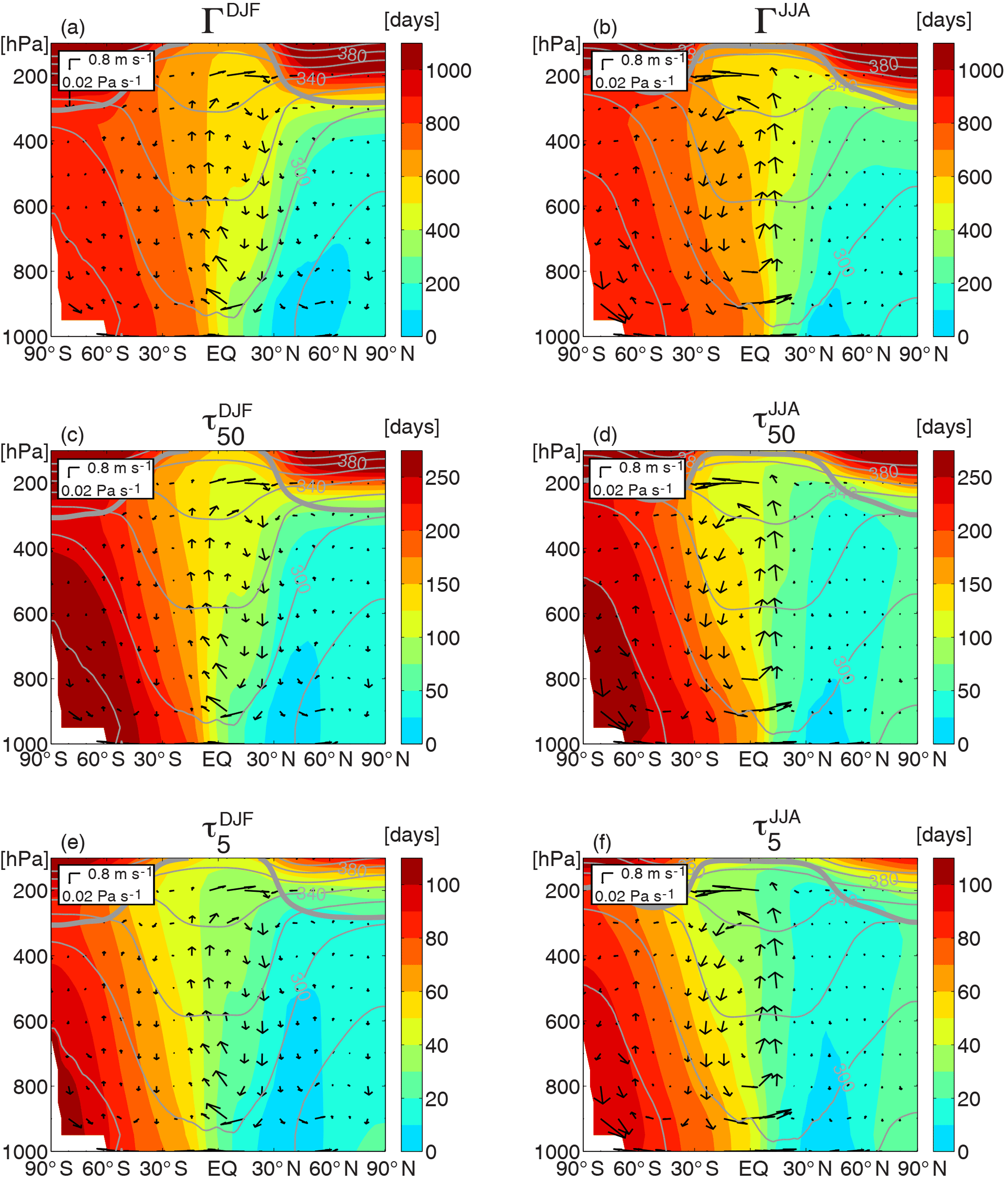
Figure 1Latitude–pressure distribution of the climatological seasonal-mean zonal-mean (a, b) Γ, (c, d) τ50, and (e, f) τ5, for boreal winter (DJF) and boreal summer (JJA). Arrows show the meridional circulation, thin contours show isentropes (contours every 20 K), and the thick contour shows the tropopause.
We first examine the climatological seasonal-mean distributions of the tracer ages, and the connection of these distributions with the general circulation. Figure 1 shows the zonally averaged Γ, τ50, and τ5 for northern winter (DJF) and summer (JJA). There is a similar distribution for the different tracer ages, with the smallest values in northern midlatitudes (close to the source region), oldest surface values at the South Pole, weak meridional gradients in northern extratropics, largest meridional gradients in tropics, and relative weak vertical gradients at all latitudes (with slightly positive vertical gradients in the NH and slightly negative gradients in the SH). The spatial distribution of the tracer age shown in Fig. 1 is similar to the distribution of idealized or realistic long-lived tracers shown in previous studies (e.g., Denning et al., 1999; Holzer and Boer, 2001; Miyazaki et al., 2008; Waugh et al., 2013) and can be related to the general circulation (e.g., Hadley cells and Intertropical Convergence Zone, ITCZ). There is rapid transport from the NH midlatitude surface into the NH extratropical troposphere, through a combination of along-isentropic and convective mixing, and as a consequence there are weak age gradients in the NH extratropics. There is also rapid low-level transport from NH midlatitudes into the tropics, but the transport into the SH is “slowed” by convection and rapid vertical mixing associated with the ITCZ, resulting in large surface meridional age gradients near the ITCZ. The rapid vertical mixing within tropical convection results in very weak vertical tracer gradients within the tropics, and the strong meridional gradients in the tropics persist into the middle troposphere. In the tropical upper troposphere there is increased meridional transport due to the upper branch of the Hadley cell, and this results in weaker meridional tracer gradients.
While there is qualitative agreement in the spatial distributions of the different tracer ages, there are substantial quantitative differences. First, there are large differences in the magnitude of the ages, especially in the SH where (consistent with Eq. 5). Second, there are differences in the meridional gradients: the meridional gradients of Γ in the tropics are much larger than those in the SH (where Γ is nearly constant), whereas the meridional gradients of τ5 are similar in the tropics and SH. These differences are illustrated in Fig. 3a and b, which show the latitudinal variation of the tracer ages at 900 hPa for DJF and JJA.
These quantitative differences among the tracer ages occur because the TTDs in the tropics and SH are very broad (Holzer and Waugh, 2015; Orbe et al., 2016), and the tracers are sensitive to different aspects of the TTDs. As discussed above, τ5 is most sensitive to the shorter transit times whereas Γ is the mean of the TTD and is dependent on the long tail of old transit times. The differences in meridional gradients of the two ages are related to changes in the shape of the TTD with latitude. Orbe et al. (2016) showed there is a transition in shape of the TTD from north of the ITCZ to south of the ITCZ, which they attributed to a change in the relative contribution of rapid advective pathways from northern midlatitudes and slow eddy-diffusive recirculation of “old” air into the tropics from the SH. The latter has a much larger impact on Γ than on τ5, resulting in a much larger increase in Γ across the ITCZ but relatively constant values in the southern extratropics. By comparison, τ5 is most sensitive to very short transit times as it is determined more by rapid advective pathways, resulting in roughly constant meridional gradients of τ5 throughout the SH.
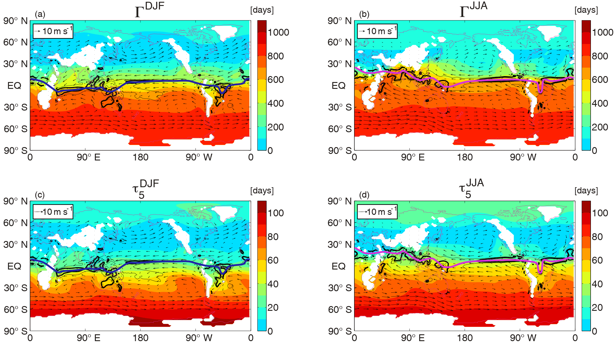
Figure 2Climatological mean Γ and τ5 at 900 hPa for (a, c) DJF and (b, d) JJA. Arrows show horizontal velocity, black contours convergence at 900 hPa (contours at (−3, −2, −1) ×106 s−1, with −2 ×10⁶ s−1 bold), and blue and pink curves show the approximate location of the ITCZ.
The latitudinal gradients in the tracers are much larger than zonal gradients, but there are still some zonal variations. This is illustrated in Fig. 2, which shows the 900 hPa distribution of the climatological Γ and τ5 for (a, c) DJF and (b, d) JJA. There are weak zonal variations in the extratropics for both tracers, but noticeable zonal variations within the tropics. For example, in DJF the mean age over the equatorial Indian Ocean is smaller than over the Equator of other oceans, whereas in JJA the mean over the northern tropical Indian Ocean is larger than over the Pacific or Atlantic oceans. These variations in the tracers can again be related to variations in meteorology. In particular, the large seasonal variation over the tropical Indian Ocean is related to seasonal changes in convection and wind direction associated with the South Asian monsoon (i.e., there is deep convection over the equatorial Indian Ocean and northerly surface winds in DJF), whereas the deep convection is over the northern subtropics and there are southerly winds in JJA.
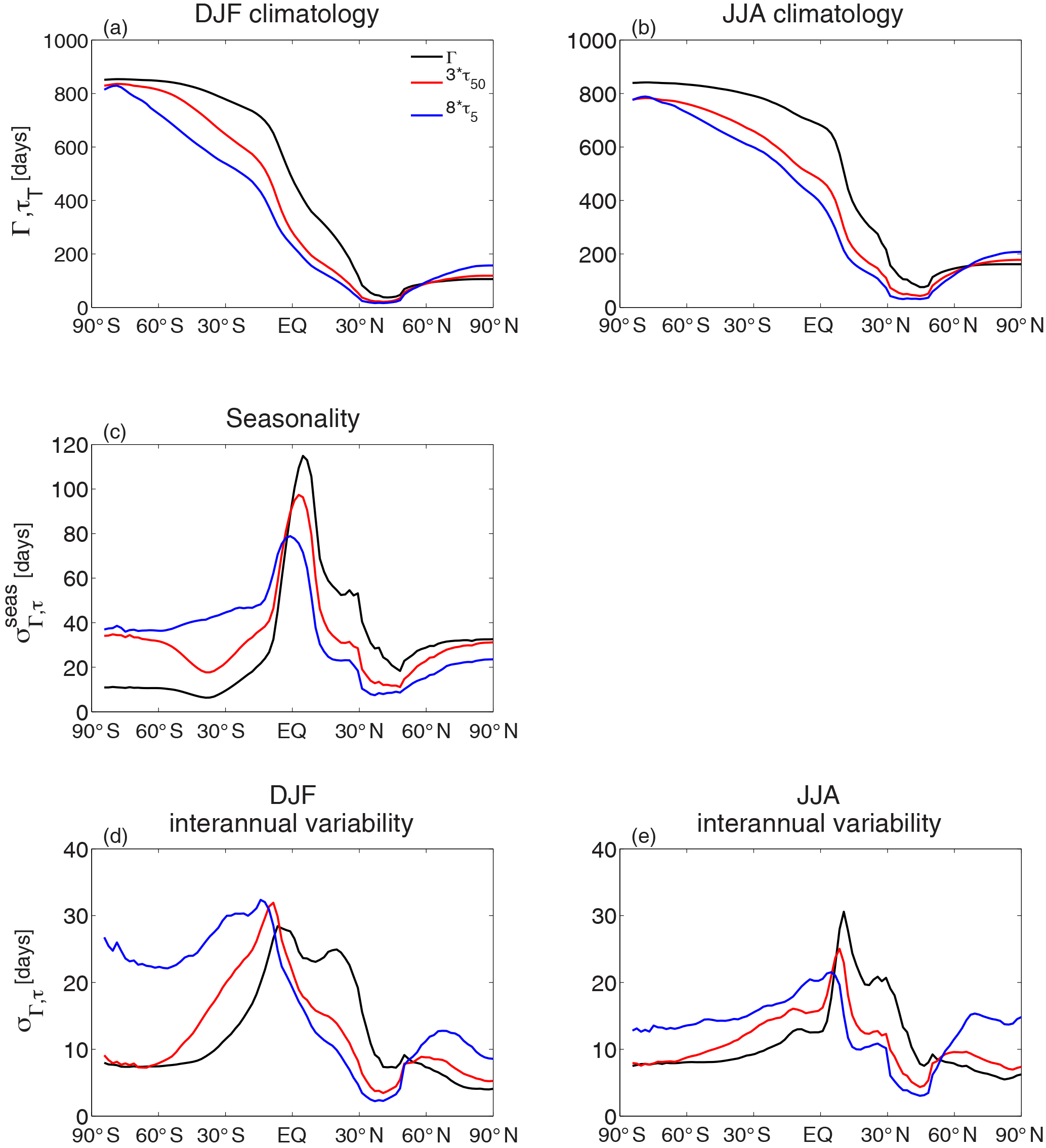
Figure 3Latitudinal variation of (a) DJF climatological mean, (b) JJA climatological mean, (c) seasonal standard deviation, (d) DJF interannual standard deviation, and (e) JJA interannual standard deviation for Γ, τ50, and τ5 at 900 hPa. For all panels the quantity for τ50 is multiplied by 3 and that for τ5 multiplied by 8.
We now examine the seasonality of the tracer ages in more detail. Previous studies have linked seasonal differences in the distributions of tracer to the seasonally varying Hadley circulation (e.g., Bowman and Cohen, 1997; Bowman and Erukhimova, 2004), and we examine this connection for the tracer ages.
Comparison of the left and right panels of Fig. 1 shows seasonal differences in all three tracer ages: the location of the largest surface meridional gradients are south of the Equator during DJF but north of the Equator during JJA, and the near-surface tracer ages at the Equator and in the southern tropics are younger in DJF than in JJA (see also Fig. 3a, b). There are also seasonal differences away from the surface, with older ages in DJF than in JJA in both northern and southern subtropical middle–upper troposphere.
As expected, these seasonal differences in the tracer ages are linked to the seasonal variations is the Hadley circulation and location of the ITCZ. The largest surface age gradients occur at the ITCZ, with young ages north of the ITCZ and older ages south. The latitude of the ITCZ moves with season and there is a corresponding north–south shift in the latitude of large meridional age gradients; i.e., largest surface meridional gradients are south of the Equator during DJF but north of the Equator during JJA (Figs. 1, 3a, b). This results, as will be shown below, in a large seasonality at locations within the seasonal range of the ITCZ, with older ages when the ITCZ is north of the location and younger ages when it is to the south.
The seasonality of the Hadley circulation can also explain the seasonality in the tracers in the northern subtropical middle troposphere and southern tropical upper troposphere. During DJF the northern cell is strongest (see arrows in Fig. 1a) and transports “older” ages from the equatorial upper troposphere into the northern subtropical middle troposphere (resulting in older ages in DJF than JJA), whereas during JJA the stronger southern cell (Fig. 1b) increases the transport of “young” air into the southern subtropical upper troposphere (again resulting in older ages in DJF than JJA).
As with the climatological distributions, there are quantitative differences in the seasonality (DJF–JJA differences) of the different tracer ages. In particular, the seasonality of near-surface Γ south of 20∘ S is much smaller than at the Equator, whereas for near-surface τ5 there is a smaller decrease in the seasonality from the Equator to southern midlatitudes. This can be seen clearly in Fig. 3c, which shows the latitudinal variation in the seasonal standard deviation .
As mentioned in the previous section, there are zonal variations in the tracer ages within the tropics that vary with season. Again, these zonal variations in the ages are consistent with variations in the ITCZ (see surface winds (arrows) and convergence (contours) in Fig. 2). The ITCZ is close to the Equator in both DJF and JJA over the Pacific, whereas there is a large seasonal variation of ITCZ over the Indian Ocean: it is well north of the Equator during JJA but south of the Equator in DJF. Similar variations occur for the regions of largest meridional age gradients. Associated with the seasonal movement of the ITCZ, there is a change in direction of the surface winds, with the largest changes again occurring in the Indian Ocean sector. In particular, in the tropical western Indian Ocean there is a strong southward flow during DJF, but a strong northward flow in JJA. This seasonality in wind direction results in a large seasonality in the age.
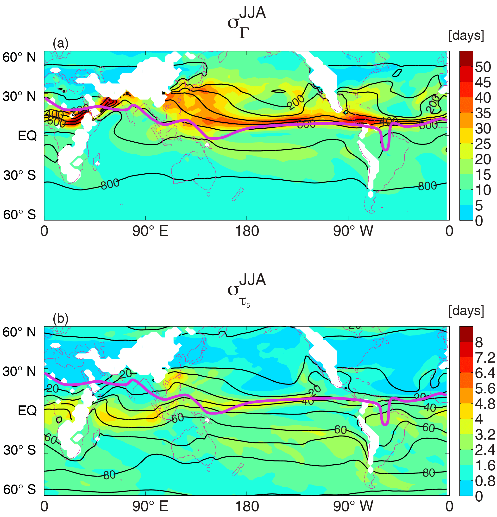
The spatial variation of the seasonality, and differences between Γ and τ5, can be seen clearly in Figs. 4 and 5, which show maps of surface and vertical cross sections, respectively, of the seasonal standard deviation . Consistent with the above discussion, the largest values of both and are within the tropics. However, while the peak and occur at similar latitudes over the Pacific and Atlantic oceans, the peak is south of the peak in the Indian Ocean sector. Also, in the southern extratropics is much smaller than in the tropics ( is as high as 180 days in the tropics but only around 10 days in the southern extratropics), whereas is comparable in the tropics and southern extratropics (5–10 days). Figure 5 also shows that large seasonality is generally only near the surface (pressures above 800 hPa). However, there is larger seasonality in the northern subtropical mid-troposphere, southern subtropical upper troposphere over the Indian Ocean, and near the tropopause (especially for τ5).
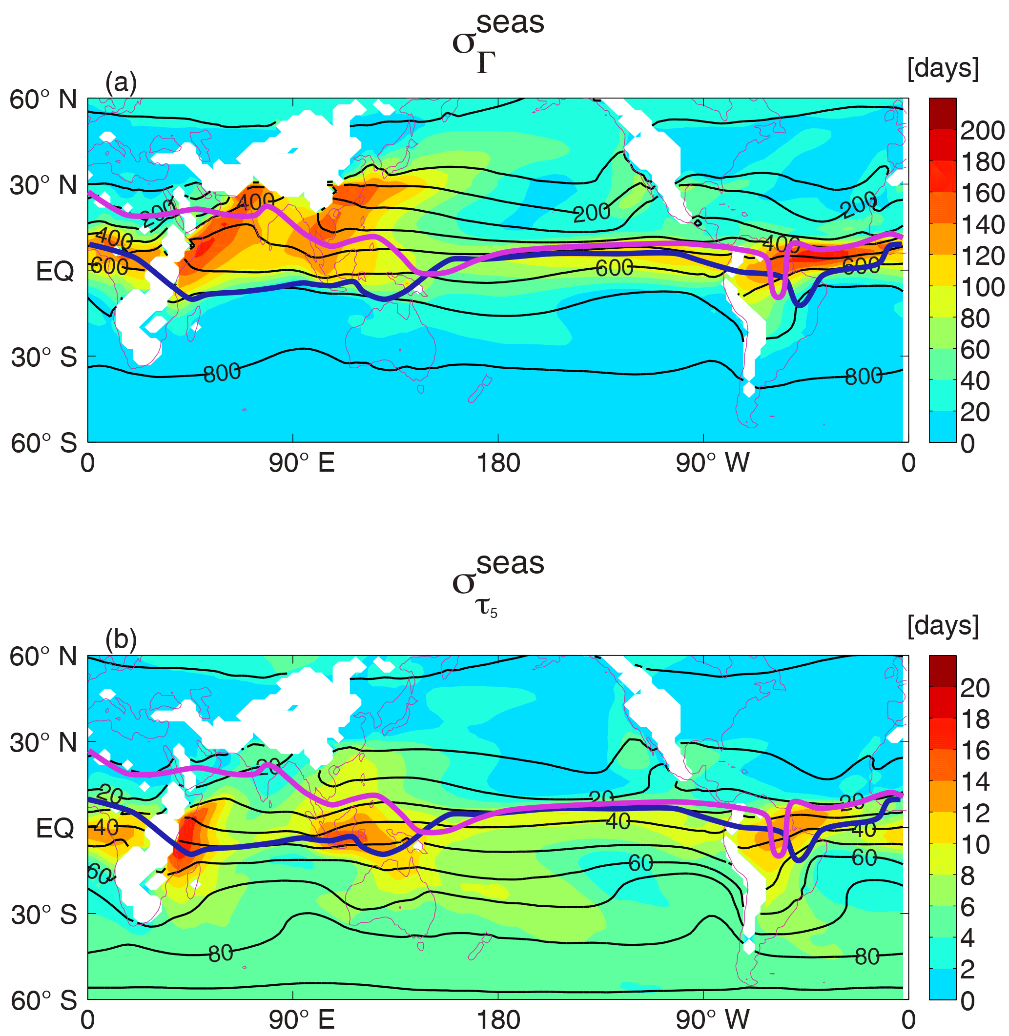
Figure 4Maps of seasonal variability of (a) Γ and (b) τ5 at 900 hPa. Thin contours show climatological mean tracer ages (in days), and blue and pink curves show approximate location of the ITCZ in DJF and JJA, respectively.
The seasonal movement of convergence zones can explain much of the seasonality in the tracer ages. In particular, the north–south movement of the ITCZ results in a similar movement of the region of high meridional age gradients and large seasonality of tracer age for tropical locations; i.e., when the ITCZ is displaced south from its climatological location there will be a decrease in the tracer age, and vice versa for a northward shift (Lintner et al., 2004). The seasonal migration of the ITCZ varies with longitude, with a much larger variation over the Indian Ocean than over the eastern Pacific (e.g., Waliser and Gautier, 1993; Gloor et al., 2007). This is shown by contours in Figs. 2 and 4; it results in a wider range of latitudes that the ITCZ crosses during the annual cycle and hence larger seasonality in tracer ages over the Indian Ocean than over the eastern Pacific (Fig. 4).
Seasonality in surface convergence also contributed to the region of enhanced seasonal variability in the subtropical western south Pacific. The South Pacific Convergence Zone (SPCZ) lies within this region, and the orientation and intensity of the SPCZ vary on synoptic through to interannual timescales (e.g., Matthews, 2012; Niznik and Lintner, 2013). This variability in the SPCZ then results in variability in tracer ages; e.g., when the SPCZ is shifted to the northeast from its climatological there is less rapid transport from the NH and more from SH middle latitudes, resulting in older ages.
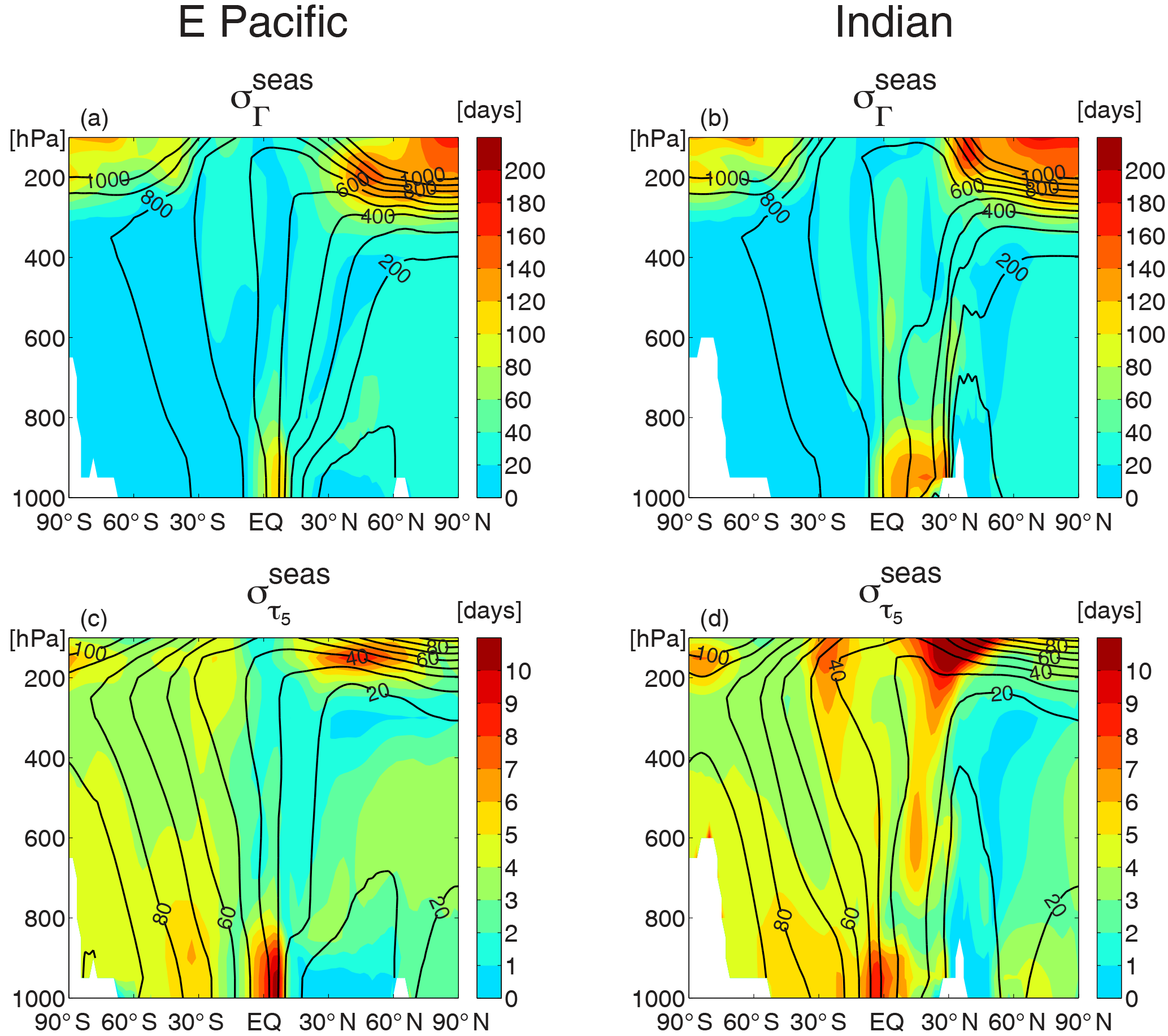
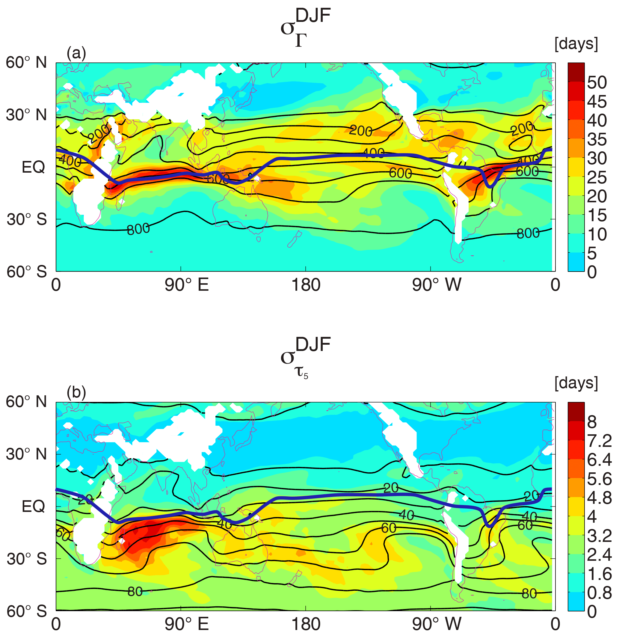
Figure 5Latitude–pressure variation of (a, b) Γ and (c, d) τ5, for eastern Pacific (150–120∘ W) and Indian Ocean (60–90∘ E) sections. Contours show climatological mean distributions of (a, b) Γ and (c, d) τ5 (in days).
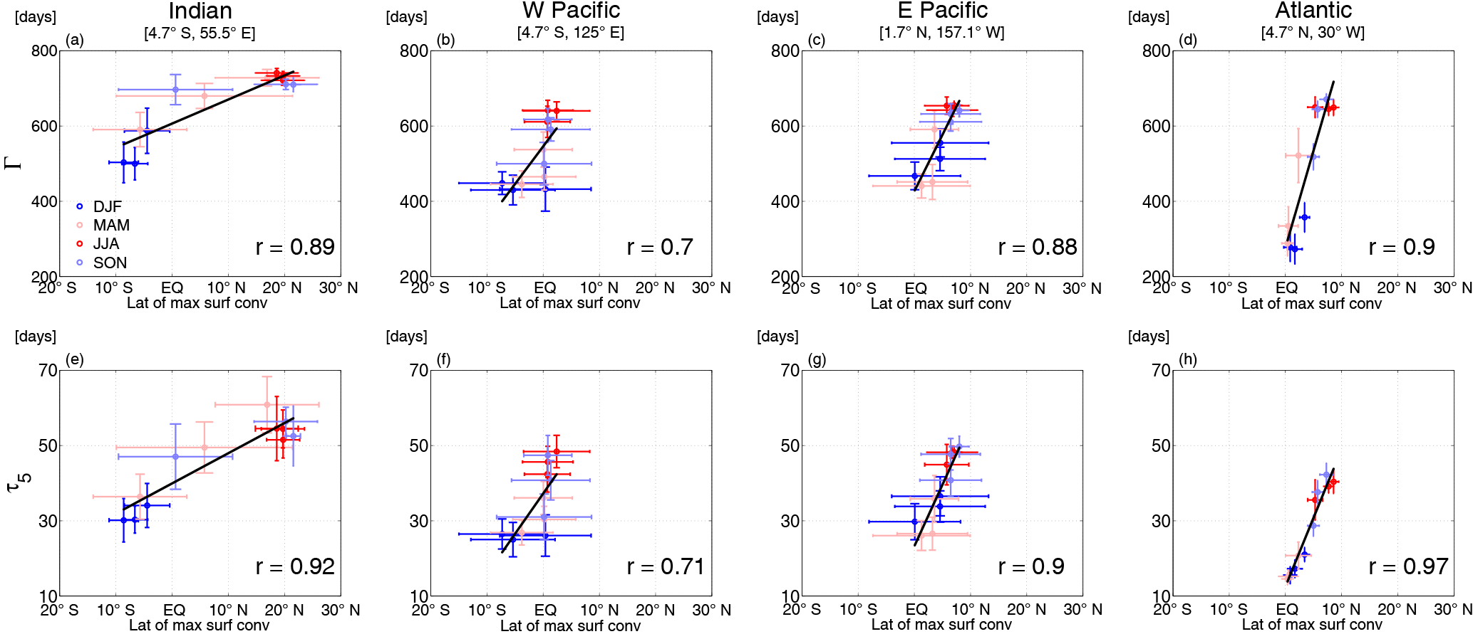
Figure 6Relationship between the latitude of maximum surface convergence and tracer age at 900 Pa for locations in the (a, e) Indian, (b, f) western Pacific, (c, g) eastern Pacific, and (d, h) Atlantic oceans. Top row shows Γ and bottom row τ5. Coordinates of the locations are shown above (a)–(d). Width of the horizontal or vertical bars are twice the interannual standard deviation, and different colors represent different seasons (see a). Black line shows linear fit, and correlation coefficient is given within each plot.
To quantify the age–ITCZ relationship we compare the latitudinal movement of the ITCZ with the age at a fixed location. Figure 6 shows the relationship between the simulated 900 hPa Γ or τ5 and the ITCZ latitude (calculated as the latitude of maximum convergence at 900 hPa between 15∘ S and 30∘ N for each longitude) for four different longitudes (corresponding to the Indian, western Pacific, eastern Pacific or Atlantic oceans). For both tracer ages and all locations there is a positive correlation, i.e., older age for a more northern location of the ITCZ. There are some differences in the age–ITCZ relationships between the ocean basins, with a more linear relationship over the Atlantic and eastern Pacific than other regions. Over the Indian Ocean the age–ITCZ relationship is nonlinear, especially for Γ, with a more rapid change of age with latitude of the ITCZ when the ITCZ is south of 10∘ N than north.
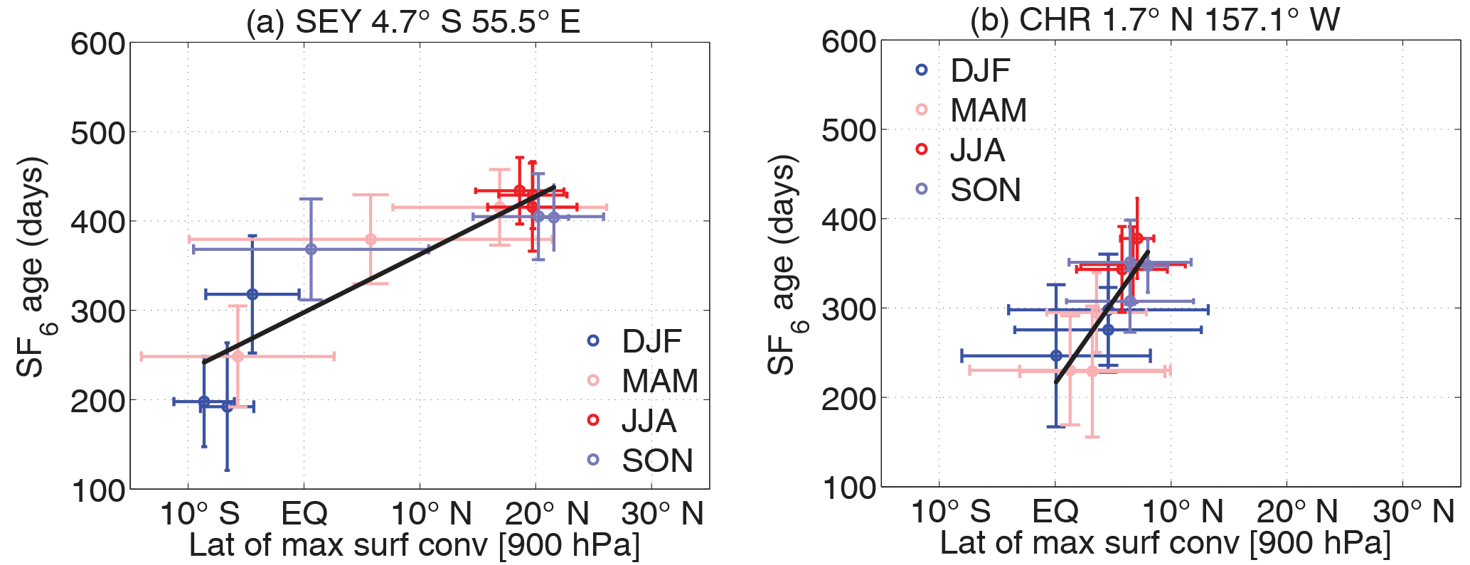
Observational evidence for the above relationship between the seasonality of tracer ages and latitude of the ITCZ is found in the measurements of SF6 from surface stations. Waugh et al. (2013) showed that a “SF6 age”, which is an approximation of the ideal age, can be estimated from measurements of SF6. There are large annual cycles of SF6 age derived from measurements in the tropical Indian (Mahé Island, Seychelles; 4.7∘ S, 55.5∘ E) and eastern Pacific (Christmas Island; 1.7∘ N, 157.1∘ W) oceans, and the variation of the SF6 age with latitude of ITCZ at these stations (Fig. 7) is similar to those for the simulated Γ (Fig. 6a, c), including the linear relationship for the eastern Pacific station but nonlinear relationship for the Indian Ocean station. Unfortunately, there are no stations within the tropical western Pacific or Atlantic to test the simulated seasonality in these regions.
We now examine the interannual variability of the tracers, first for northern winter (DJF) and then northern summer (JJA).
5.1 Northern winter
Given the above relationship between seasonal variability of tropical convergence zones and tracer ages, we expect the interannual variations of the tracer ages to be largest near these convergence zones. As shown in Fig. 8, this is indeed the case for DJF, with largest variance generally around or south of the ITCZ (contours) and SPCZ (not marked). The interannual variability is weaker than the seasonality, e.g., the maximum is around 50 days compared to 180 days for , and there are also differences in the locations of peak seasonal and interannual variability. For example, the peak over the Indian sector is in the central equatorial Indian Ocean, whereas the peak is north of the Equator (with two local maxima). A similar difference in locations of peak values occurs between and , and the tropical–extratropical difference in is much smaller than that for (see also Fig. 3). Again consistent with seasonal variability, the interannual variability is largest near the surface and generally small in the upper troposphere (not shown).
The El Niño–Southern Oscillation (ENSO) is the major cause of interannual variability in low-latitude meteorology, and previous studies have shown that variability in interhemispheric transport is linked to ENSO (e.g, Elkins et al., 1993; Prinn et al., 1992; Lintner et al., 2004; Waugh et al., 2013). We examine this relationship here by calculating the correlation r and regression m coefficients between the 30-year times series of DJF Γ at each location and the Oceanic Niño Index (ONI).
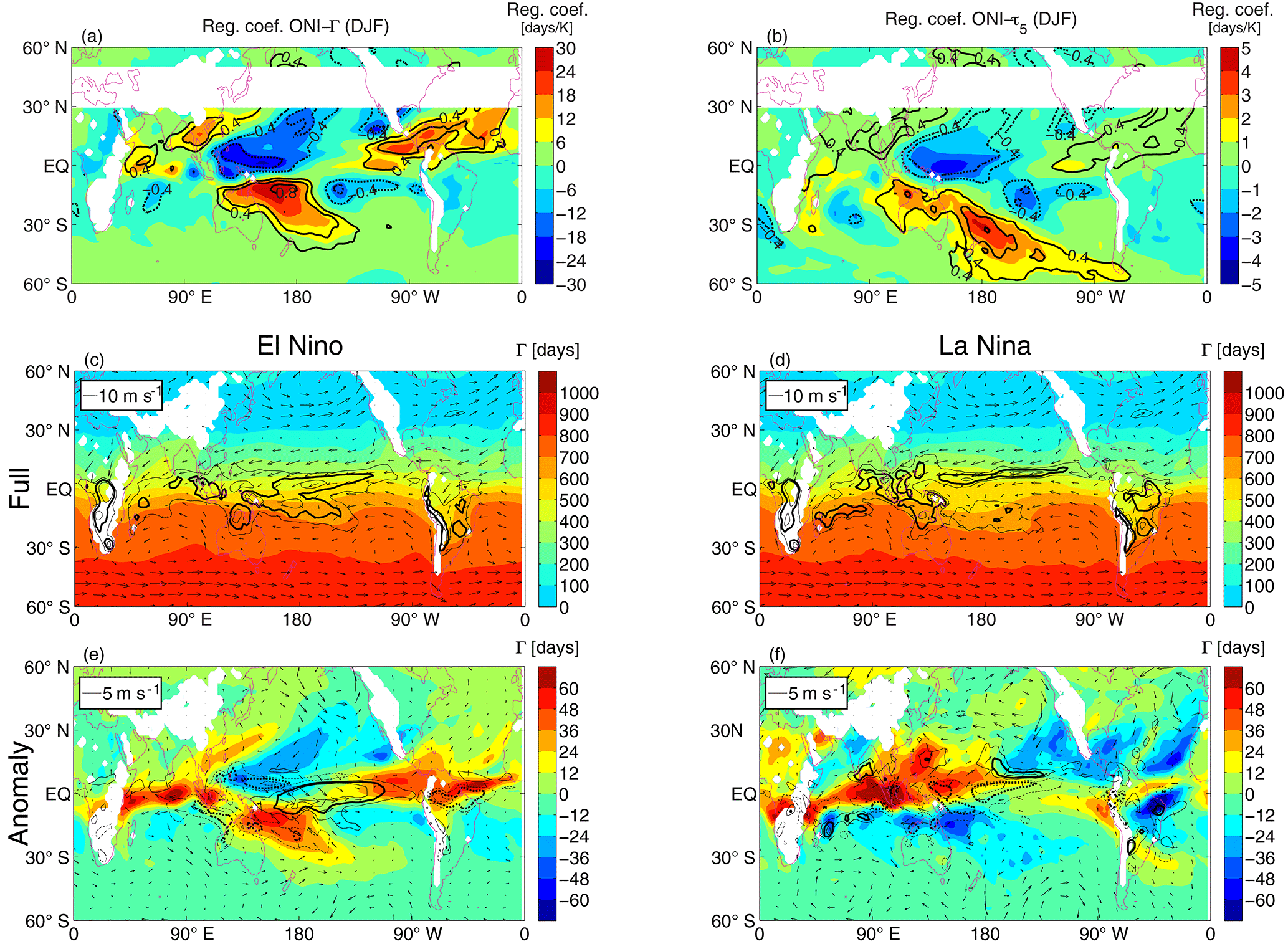
Figure 9Relationships between tracer ages and ENSO. (a) Regression coefficients (shading) and correlation coefficients (contours) between Γ at 900 hPa and ONI for DJF. Correlations with absolute value larger than 0.361 are significant at 95 % confidence level. (b) As in (a) but for τ5 at 900 hPa. (c, d) Γ (shading), 900 hPa horizonal winds (arrows) and precipitation (contours; (4, 6, 8) mm day−1, with the 6 mm day−1 bold) for composites of (c) El Niño winters and (d) La Niña winters. (e, f) As in panels (c, d) but showing the anomaly from climatological DJF fields. In panel (e) black contours show precipitation anomalies of (4, 6, 8) mm day−1, and gray contours show precipitation anomalies of (−8, −6, −4) mm day−1 while in panel (f) black contours show precipitation anomalies of (2, 3, 4) mm day−1, and gray contours show precipitation anomalies of (−4, −3, −2) mm day−1.
Figure 9a show maps of the regression coefficients (shading) and correlation coefficients (contours) for the Γ–ENSO relationship. There are coherent regions with large positive or negative correlations in both hemispheres, with correlations north of the Equator generally the opposite sign to those south of the Equator at the same longitude. There is large region with positive correlation in the southern subtropical central Pacific (near 170∘ E), but negative correlations are found in southern subtropical eastern Pacific and Indian oceans. Thus, during an El Niño year there tends to be older ages over the southern subtropical central Pacific but younger ages over the southern subtropical eastern Pacific and Indian oceans, and the reverse for La Niña years. The Γ–ENSO correlations at and north of the Equator are generally the opposite sign to those south of the Equator at the same longitude; i.e., there are negative correlations in northern tropical central Pacific. A similar pattern of correlations with ENSO is also found for τ5, with, consistent with the above analysis, the region of largest correlations slightly south of that for correlation with Γ (Fig. 9b).
The above Γ–ENSO correlations are example further by considering composites of Γ and meteorological fields for El Niño years (ONI greater than 1) and La Niña years (ONI less than −1). Figure 9b–e show maps of DJF Γ, CAM-C1SD precipitation (as a proxy for the intensity of tropical convection), and surface winds for the El Niño and La Niña composites; in panels b and c the full fields are shown whereas in panels d and e the anomalies from the 30-year climatology are shown. These maps show a difference in the location of the region of high precipitation (ITCZ) over the tropical Pacific between ENSO phases: during El Niño years the ITCZ is south of its location during La Niña years (around 5∘ S compared to around ∼ 10∘ N). This results in differences in transport to the equatorial western-central Pacific. During El Niño years there is rapid, direct low-level transport to the Equator, whereas for La Niña years the convection around 10∘ N reduces this direct transport and the Γ is older in the same region (consistent with the negative correlation shown in Fig. 9a). The reverse Γ–ENSO correlation occurs in the southern tropical Pacific because of interannual variations in the SPCZ. During most winters the SPCZ is orientated diagonally in the northwest to southeast direction, but during some strong El Niño events the SPCZ is shifted north and is more zonally orientated (Vincent et al., 2011). During these El Niño years there is less rapid transport of younger air from the NH and older air from the SH high latitudes, and hence older tracer ages, in the southwestern tropical Pacific.
The signs of the age–ENSO correlations over the eastern Pacific, Atlantic and Indian oceans are opposite to that over the western-central Pacific; i.e., there is positive correlation in the northern tropics over eastern Pacific but a negative correlation over the western Pacific (Fig. 9a). The cause of this is not clear, although it likely due to El Niño–La Niña differences in the subtropical surface flow over these regions. For example, during El Niño years the equatorial winds over the equatorial Indian Ocean have a stronger than average northward component, which transport more old, southern hemispheric air across the Equator, resulting in older age in the northern tropical Indian Ocean.
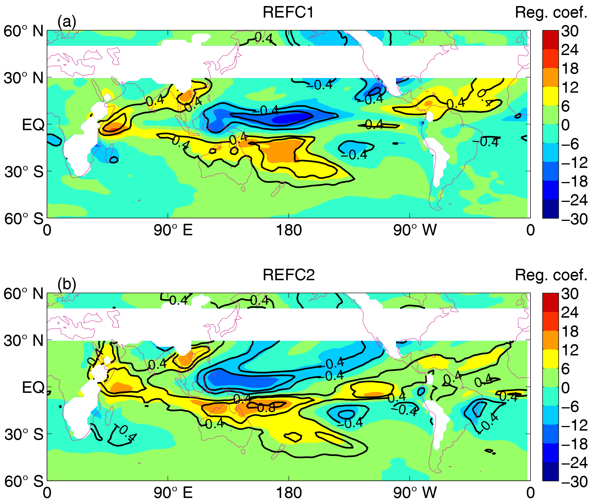
Some caution is needed with the simulated age–ENSO relationship as it is based only on a 30-year simulation. However, analysis of the Γ–ENSO relationship in two free-running CAM4-chem simulations yields very similar regression patterns, including high negative and positive correlations either side of the Equator in western-central Pacific and the opposite signed correlations over the eastern Pacific and Indian oceans; see Fig. 10. (In the “REFC1” simulation CAM4-chem is constrained by observed sea surface temperatures and sea ice concentrations, whereas “REFC2” is a simulation where the atmosphere is coupled to dynamic ocean and sea ice models.)
Observational support for the above age–ENSO correlation is found in trace gas measurements at American Samoa (14∘ S, 170∘ W). Measurements of methyl chloroform and CFCs from this station show lower concentrations (indicating slower transport from NH sources) during El Niño years (e.g, Elkins et al., 1993; Prinn et al., 1992). As American Samoa lies just inside the region of positive age–ONI correlation, this is consistent with the above simulated variability. The simulations indicate that the observed result of slower transport to the SH during El Niño years may hold only in the western-central Pacific, and there could be faster transport to the eastern Pacific or Indian subtropical oceans. Unfortunately similar multi-year trace gas measurements are not available from these locations to test this.
Although ENSO explains much of the variability in the Pacific this is not the case for other basins. In particular, the largest interannual variability of Γ and τ5 occurs over the southern tropical Indian Ocean, but variability here is only weakly correlated with ENSO. The interannual of the tracers is still related to changes in location of surface convergence and direction of surface winds, but this variability surface flow is not correlated with ENSO or with the Indian Ocean Dipole (not shown). Further analysis is required to determine the causes of the interannual variability of the flow and transport in the Indian Ocean.
5.2 Northern summer
The general characteristics of the interannual variability during northern summer (JJA) are similar to that in winter; i.e., the largest variability is in the tropics and there is small variability in the SH (especially for Γ) (see Fig. 11a and b). However, the location of the peak interannual variability at the surface varies between seasons, with the peak in generally north of that for . This is consistent with the more northern location of the ITCZ in JJA; i.e., the peak standard deviation for each season is close to the climatological location of the ITCZ for that season. As in DJF, the largest is located south of peak . This is especially true in the Indian Ocean sector, where is largest around 20∘ N but is largest around 5∘ S. This difference between the tracer ages is again consistent with the differences in their meridional gradients; e.g., there are weak Γ gradients in the tropical Indian Ocean but large τ5 gradients in southern tropics.
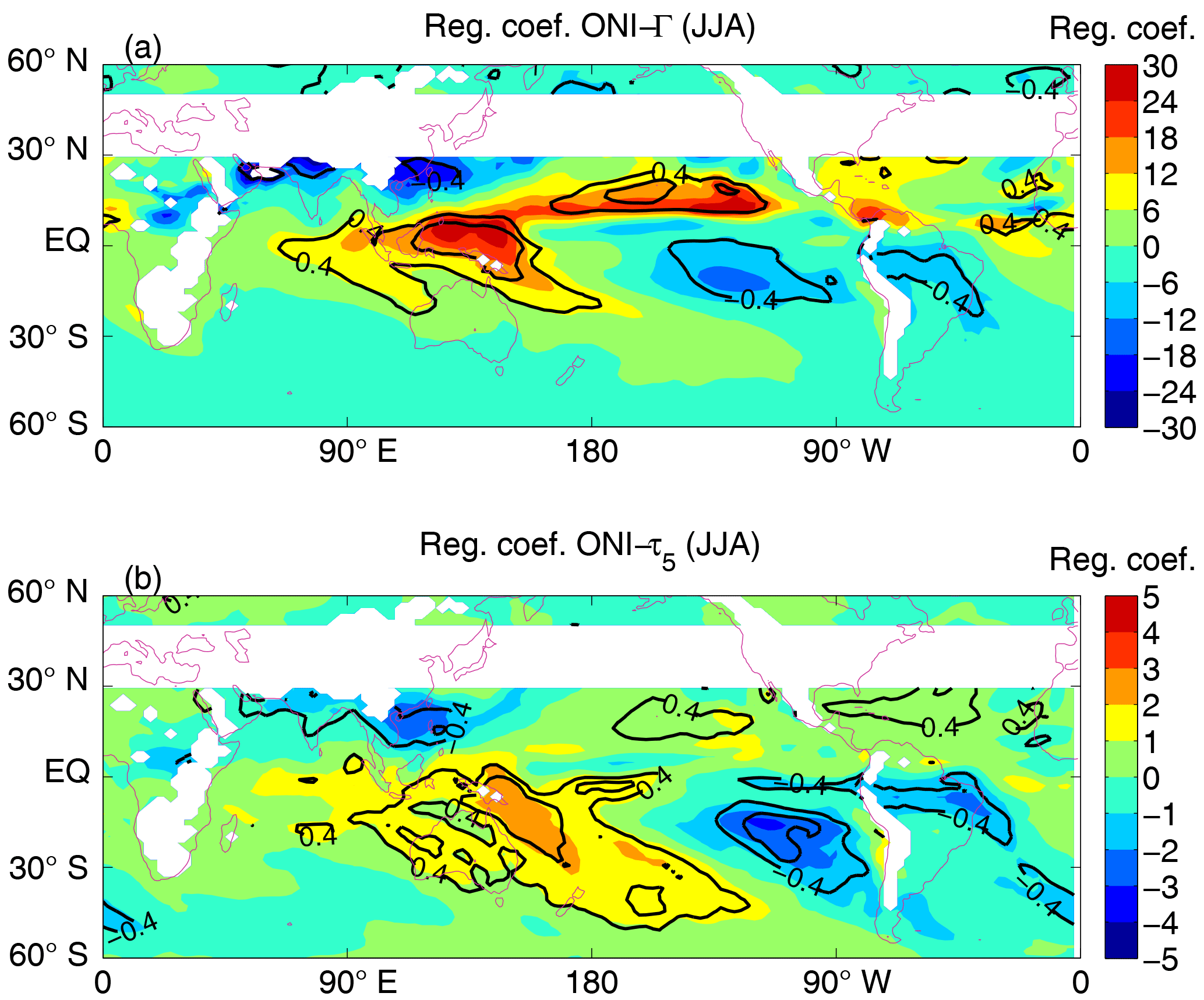
Some of the interannual variability in JJA tracer ages is correlated with ENSO, with older ages over the northern central tropical Pacific and southern subtropical eastern Pacific and younger ages over southeastern Asia during the warm phase (El Niño); see Fig. 12. However, as in DJF, this applies mainly to the Pacific ocean and ENSO is not the dominant source of variability over the Indian and Atlantic oceans.

While the variability of the tracer ages generally decreases with height from the surface, this is not the case for over the western tropical Indian Ocean. Here there is very little interannual variability near the surface for this region, but as shown in Fig. 13 there is a region of high interannual variability at 650 hPa that extends from tropical Africa over the Indian Ocean. Near the surface the largest occurs around 30∘ N, but around 650 hPa the largest variability is around 5∘ N. The large near the surface can be attributed to the variations of ITCZ (surface convergence), but variability in the ITCZ does not account for the large variability near 650 hPa. A possible cause of the large at 650 hPa is variability in the ascent in the lower–middle troposphere over this region. During JJA there is a narrow region of strong ascent in the lower–middle troposphere over tropical Africa and the Indian Ocean, between the African easterly jet and tropical easterly jet, that does not extend down to the surface but does produce large precipitation in a “tropical rain belt” south of the surface ITCZ (e.g., Nicholson, 2009). This region of strong ascent likely impacts meridional tracer transport, and the large at 650 hPa could be connected to variability in ascent. This possibility requires further examination.
The seasonal and interannual variability of transport times from the NH midlatitude surface into the tropics and SH has been examined using simulations of idealized “age” tracers. For all tracers the largest seasonal and interannual variability occurs near the surface within the tropics and is generally closely coupled to variability in the tropical convergence zones (ITCZ, SPCZ). The seasonal migration of the ITCZ is responsible for the majority of seasonality in the tracer ages (with younger ages when the ITCZ is further south), while a large amount of the interannual variability during DJF is due to ENSO-related variations in surface convergence and convection, especially over the Pacific Ocean. Trace gas observations from surface stations provide support for these model results: the “SF6 age” derived from tropical measurements varies seasonally with the latitude of the ITCZ in a similar manner to the simulated ideal age, and lower concentrations of tracers with NH sources are observed at the American Samoa station during El Niño years (consistent with slower transport).
There are, however, notable differences in the variability of tracers with different time dependencies. The largest variability in the mean age (Γ) is confined to the tropics, generally close to the location of the ITCZ (or SPCZ), and there is very weak seasonal or interannual variability in the southern extratropics (e.g., the interannual standard deviation of Γ in the southern extratropics is less than 1 % of the climatological mean value). In contrast, for the 5- and 50-day loss tracers the peak variability of the tracer age tends to be south of the ITCZ, and there is a smaller contrast between tropical and extratropical variability. For example, the DJF interannual standard deviation of the age of the 5-day loss tracer (τ5) is around 30–40 % of the mean in both the tropics and southern midlatitudes.
These differences in temporal variability of the tracers occur because the tracers are sensitive to different aspects of the TTD (e.g., τ5 is more sensitive to changes in the fast transit times than Γ), and this results in differing meridional age gradients. Orbe et al. (2016) noted that fast (advective) transport pathways make only a very small contribution to the TTD south of the ITCZ, and the TTD is dominated by slow (eddy-diffusive) pathways. Changes in these fast transport pathways south of the ITCZ can cause substantial variations in tracers with rapid loss (e.g., τ5) as these tracers are sensitive to changes in the fast timescales (and insensitive to changes in transit times much longer than a month as these carry little tracer), but have much weaker impact of the mean transit time (which is more strongly influenced by the tail of the TTD).
The differing seasonal and interannual variability of the idealized tracers suggests that the seasonal–interannual variability in the southern extratropics of trace gases, with predominantly NH sources, may differ depending on the chemical lifetimes of the gases. For tracers with very long lifetimes (e.g., SF6 and CFCs) we may expect very weak temporal variability due to transport, whereas for tracers with shorter lifetimes (e.g., non-methane hydrocarbons) there may be noticeable transport-induced seasonal or interannual variability. Conversely, our study also suggests that combinations of tracers with different lifetimes may be used to constrain the TTD from observations. This possibility requires further examination.
The CAM4chem output can be downloaded from https://www.earthsystemgrid.org/search.html?freeText=ccmi1 (last access: January 2017) and the ONI data from http://www.cpc.ncep.noaa.gov/ (last access: August 2016).
The authors declare that they have no conflict of interest.
This article is part of the special issue “Chemistry-Climate Modelling Initiative (CCMI) (ACP/AMT/ESSD/GMD inter-journal SI)”. It is not associated with a conference.
This work was supported by NSF Grant AGS-1403676 and NASA Grant
NNX14AP58G.
Edited by: Peter Hess
Reviewed by: two anonymous referees
Bowman, K. P.: Transport of carbon monoxide from the tropics to the extratropics, J. Geophys. Res.-Atmos., 111, https://doi.org/10.1029/2005JD006137, 2006. a
Bowman, K. P. and Carrie, G. D.: The mean-meridional transport circulation of the troposphere in an idealized GCM, J. Atmos. Sci., 59, 1502–1514, 2002. a, b
Bowman, K. P. and Cohen, P. J.: Interhemispheric exchange by seasonal modulation of the Hadley circulation, J. Atmos. Sci., 54, 2045–2059, 1997. a
Bowman, K. P. and Erukhimova, T.: Comparison of global-scale Lagrangian transport properties of the NCEP reanalysis and CCM3, J. Climate, 17, 1135–1146, 2004. a, b
Deleersnijder, E., Delhez, E., and Beckers, J.: Some properties of generalized age-distribution equations in fluid dynamics, SIAM J. Appl. Math., 61, 1526–1544, 2001. a
Denning, A. S., Holzer, M., Gurney, K. R., Heimann, M., Law, R. M., Rayner, P. J., Fung, I. Y., Fan, S. M., Taguchi, S., Friedlingstein, P., and Balkanski, Y.: Dimensional transport and concentration of SF6, Tellus B, 51, 266–297, 1999. a, b
Elkins, J., Thompson, T., Swanson, T., Butler, J., Hall, B., Cummings, S., Fisher, D., and Raffo, A.: Decrease in the growth rates of atmospheric chlorofluorocarbons 11 and 12, Nature, 364, 780–783, 1993. a, b
Eyring, V., Lamarque, J., Hess, P., Arfeuille, F., Bowman, K., Chipperfiel, M., Duncan, B., Fiore, A., Gettelman, A., Giorgetta, M., and Granier, C.: Overview of IGAC/SPARC Chemistry-Climate Model Initiative (CCMI) community simulations in support of upcoming ozone and climate assessments, SPARC newsletter, 40, 48–66, 2013. a, b
Francey, R. J. and Frederiksen, J. S.: The 2009–2010 step in atmospheric CO2 interhemispheric difference, Biogeosciences, 13, 873–885, https://doi.org/10.5194/bg-13-873-2016, 2016. a
Geller, L. S., Elkins, J. W., Lobert, J. M., Clarke, A. D., Hurst, D. F., Butler, J. H., and Myers, R. C.: Tropospheric SF6: Observed latitudinal distribution and trends, derived emissions and interhemispheric exchange time, Geophys. Res. Lett., 24, 675–678, https://doi.org/10.1029/97GL00523, 1997. a
Gloor, M., Dlugokencky, E., Brenninkmeijer, C., Horowitz, L., Hurst, D., Dutton, G., Crevoisier, C., Machida, T., and Tans, P.: Three-dimensional SF6 data and tropospheric transport simulations: Signals, modeling accuracy, and implications for inverse modeling, J. Geophys. Res.-Atmos., 112, https://doi.org/10.1029/2006JD007973, 2007. a
Haine, T. W. and Hall, T. M.: A generalized transport theory: Water-mass composition and age, J. Phys. Oceanogr., 32, 1932–1946, 2002. a
Hall, T. M. and Plumb, R. A.: Age as a diagnostic of stratospheric transport, J. Geophys. Res.-Atmos., 99, 1059–1070, 1994. a
Holzer, M. and Boer, G. J.: Simulated changes in atmospheric transport climate, J. Climate, 14, 4398–4420, 2001. a, b, c
Holzer, M. and Waugh, D. W.: Interhemispheric transit time distributions and path-dependent lifetimes constrained by measurements of SF6, CFCs, and CFC replacements, Geophys. Res. Lett., 42, 4581–4589, 2015. a, b
Krol, M. and Lelieveld, J.: Can the variability in tropospheric OH be deduced from measurements of 1, 1, 1-trichloroethane (methyl chloroform)?, J. Geophys. Res.-Atmos., 108, https://doi.org/10.1029/2002JD002423, 2003. a
Lamarque, J.-F., Emmons, L. K., Hess, P. G., Kinnison, D. E., Tilmes, S., Vitt, F., Heald, C. L., Holland, E. A., Lauritzen, P. H., Neu, J., Orlando, J. J., Rasch, P. J., and Tyndall, G. K.: CAM-chem: description and evaluation of interactive atmospheric chemistry in the Community Earth System Model, Geosci. Model Dev., 5, 369–411, https://doi.org/10.5194/gmd-5-369-2012, 2012. a
Levin, I. and Hesshaimer, V.: Refining of atmospheric transport model entries by the globally observed passive tracer distributions of 85krypton and sulfur hexafluoride (SF6), J. Geophys. Res.-Atmos., 101, 16745–16755, 1996. a
Liang, Q., Chipperfield, M. P., Fleming, E. L., Abraham, N. L., Braesicke, P., Burkholder, J. B., Daniel, J. S., Dhomse, S., Fraser, P. J., Hardiman, S. C., Jackman, C. H., Kinnison, D. E., Krummel, P. B., Montzka, S. A., Morgenstern, O., McCulloch, A., Mühle, J., Newman, P. A., Orkin, V. L., Pitari, G., Prinn, R. G., Rigby, M., Rozanov, E., Stenke, A., Tummon, F., Velders, G. J. M., Visioni, D., and Weiss, R. F.: Deriving Global OH Abundance and Atmospheric Lifetimes for Long-Lived Gases: A Search for CH3CCl3 Alternatives, J. Geophys. Res.-Atmos., 122, https://doi.org/10.1002/2017JD026926, 2017. a
Lintner, B. R., Gilliland, A. B., and Fung, I. Y.: Mechanisms of convection-induced modulation of passive tracer interhemispheric transport interannual variability, J. Geophys. Res.-Atmos., 109, https://doi.org/10.1029/2003JD004306, 2004. a, b, c
Maiss, M., Steele, L. P., Francey, R. J., Fraser, P. J., Langenfelds, R. L., Trivett, N. B., and Levin, I.: Sulfur hexafluoride – A powerful new atmospheric tracer, Atmos. Environ., 30, 1621–1629, 1996. a
Matthews, A. J.: A multiscale framework for the origin and variability of the South Pacific Convergence Zone, Q. J. Roy. Meteor. Soc., 138, 1165–1178, 2012. a
Miyazaki, K., Patra, P. K., Takigawa, M., Iwasaki, T., and Nakazawa, T.: Global-scale transport of carbon dioxide in the troposphere, J. Geophys. Res.-Atmos., 113, https://doi.org/10.1029/2007JD009557, 2008. a, b
Montzka, S. A., Krol, M., Dlugokencky, E., Hall, B., Jöckel, P., and Lelieveld, J.: Small interannual variability of global atmospheric hydroxyl, Science, 331, 67–69, 2011. a
Nicholson, S. E.: A revised picture of the structure of the “monsoon” and land ITCZ over West Africa, Clim. Dynam., 32, 1155–1171, 2009. a
Niznik, M. J. and Lintner, B. R.: Circulation, moisture, and precipitation relationships along the South Pacific convergence zone in reanalyses and CMIP5 models, J. Climate, 26, 10174–10192, 2013. a
Orbe, C., Waugh, D. W., Newman, P. A., and Steenrod, S.: The transit-time distribution from the Northern Hemisphere midlatitude surface, J. Atmos. Sci., 73, 3785–3802, 2016. a, b, c, d, e
Orbe, C., Waugh, D. W., Yang, H., Lamarque, J.-F., Tilmes, S., and Kinnison, D. E.: Tropospheric transport differences between models using the same large-scale meteorological fields, Geophys. Res. Lett., 44, 1068–1078, 2017. a
Orbe, C., Yang, H., Waugh, D. W., Zeng, G., Morgenstern , O., Kinnison, D. E., Lamarque, J.-F., Tilmes, S., Plummer, D. A., Scinocca, J. F., Josse, B., Marecal, V., Jöckel, P., Oman, L. D., Strahan, S. E., Deushi, M., Tanaka, T. Y., Yoshida, K., Akiyoshi, H., Yamashita, Y., Stenke, A., Revell, L., Sukhodolov, T., Rozanov, E., Pitari, G., Visioni, D., Stone, K. A., Schofield, R., and Banerjee, A.: Large-scale tropospheric transport in the Chemistry-Climate Model Initiative (CCMI) simulations, Atmos. Chem. Phys., 18, 7217–7235, https://doi.org/10.5194/acp-18-7217-2018, 2018. a
Prinn, R., Cunnold, D., Simmonds, P., Alyea, F., Boldi, R., Crawford, A., Fraser, P., Gutzler, D., Hartley, D., Rosen, R., and Rasmussen, R.: Global average concentration and trend for hydroxyl radicals deduced from ALE/GAGE trichloroethane (methyl chloroform) data for 1978–1990, J. Geophys. Res.-Atmos., 97, 2445–2461, 1992. a, b
Prinn, R., Huang, J., Weiss, R., Cunnold, D., Fraser, P., Simmonds, P., McCulloch, A., Harth, C., Reimann, S., Salameh, P., and O'Doherty, S.: Evidence for variability of atmospheric hydroxyl radicals over the past quarter century, Geophys. Res. Lett., 32, https://doi.org/10.1029/2004GL022228, 2005. a
Rienecker, M. M., Suarez, M. J., Gelaro, R., Todling, R., Bacmeister, J., Liu, E., Bosilovich, M. G., Schubert, S. D., Takacs, L., Kim, G.-K., and Bloom, S.: MERRA: NASA's modern-era retrospective analysis for research and applications, J. Climate, 24, 3624–3648, 2011. a
Tilmes, S., Lamarque, J.-F., Emmons, L. K., Kinnison, D. E., Ma, P.-L., Liu, X., Ghan, S., Bardeen, C., Arnold, S., Deeter, M., Vitt, F., Ryerson, T., Elkins, J. W., Moore, F., Spackman, J. R., and Val Martin, M.: Description and evaluation of tropospheric chemistry and aerosols in the Community Earth System Model (CESM1.2), Geosci. Model Dev., 8, 1395–1426, https://doi.org/10.5194/gmd-8-1395-2015, 2015. a
Tilmes, S., Lamarque, J.-F., Emmons, L. K., Kinnison, D. E., Marsh, D., Garcia, R. R., Smith, A. K., Neely, R. R., Conley, A., Vitt, F., Val Martin, M., Tanimoto, H., Simpson, I., Blake, D. R., and Blake, N.: Representation of the Community Earth System Model (CESM1) CAM4-chem within the Chemistry-Climate Model Initiative (CCMI), Geosci. Model Dev., 9, 1853–1890, https://doi.org/10.5194/gmd-9-1853-2016, 2016. a
Vincent, E. M., Lengaigne, M., Menkes, C. E., Jourdain, N. C., Marchesiello, P., and Madec, G.: Interannual variability of the South Pacific Convergence Zone and implications for tropical cyclone genesis, Clim. Dynam., 36, 1881–1896, 2011. a
Waliser, D. E. and Gautier, C.: A satellite-derived climatology of the ITCZ, J. Climate, 6, 2162–2174, 1993. a
Waugh, D., Crotwell, A., Dlugokencky, E., Dutton, G., Elkins, J., Hall, B., Hintsa, E., Hurst, D., Montzka, S., Mondeel, D., and Moore, F. L.: Tropospheric SF6: Age of air from the Northern Hemisphere midlatitude surface, J. Geophys. Res.-Atmos., 118, 11–429, 2013. a, b, c, d
Waugh, D. W., Hall, T. M., and Haine, T. W.: Relationships among tracer ages, J. Geophys. Res.-Oceans, 108, https://doi.org/10.1029/2002JC001325, 2003. a, b, c
agetracers. The largest variability occurs near the surface close to the tropical convergence zones, but the peak is further south and there is a smaller tropical–extratropical contrast for tracers with more rapid loss. Hence the variability of trace gases in the southern extratropics will vary with their chemical lifetime.