the Creative Commons Attribution 4.0 License.
the Creative Commons Attribution 4.0 License.
 | 25 May 2018
The impact of atmospheric stability and wind shear on vertical cloud overlap over the Tibetan Plateau
Jiming Li
Qiaoyi Lv
Bida Jian
Min Zhang
Chuanfeng Zhao
Qiang Fu
Kazuaki Kawamoto
Hua Zhang
Studies have shown that changes in cloud cover are responsible for the rapid climate warming over the Tibetan Plateau (TP) in the past 3 decades. To simulate the total cloud cover, atmospheric models have to reasonably represent the characteristics of vertical overlap between cloud layers. Until now, however, this subject has received little attention due to the limited availability of observations, especially over the TP. Based on the above information, the main aim of this study is to examine the properties of cloud overlaps over the TP region and to build an empirical relationship between cloud overlap properties and large-scale atmospheric dynamics using 4 years (2007–2010) of data from the CloudSat cloud product and collocated ERA-Interim reanalysis data. To do this, the cloud overlap parameter α, which is an inverse exponential function of the cloud layer separation D and decorrelation length scale L, is calculated using CloudSat and is discussed. The parameters α and L are both widely used to characterize the transition from the maximum to random overlap assumption with increasing layer separations. For those non-adjacent layers without clear sky between them (that is, contiguous cloud layers), it is found that the overlap parameter α is sensitive to the unique thermodynamic and dynamic environment over the TP, i.e., the unstable atmospheric stratification and corresponding weak wind shear, which leads to maximum overlap (that is, greater α values). This finding agrees well with the previous studies. Finally, we parameterize the decorrelation length scale L as a function of the wind shear and atmospheric stability based on a multiple linear regression. Compared with previous parameterizations, this new scheme can improve the simulation of total cloud cover over the TP when the separations between cloud layers are greater than 1 km. This study thus suggests that the effects of both wind shear and atmospheric stability on cloud overlap should be taken into account in the parameterization of decorrelation length scale L in order to further improve the calculation of the radiative budget and the prediction of climate change over the TP in the atmospheric models.
- Article
(3593 KB) - Full-text XML
- BibTeX
- EndNote


The Tibetan Plateau (TP), which is also known as the “roof of the world” or the “world water tower”, plays a significant role in determining global atmospheric circulations, in addition to its strong influence on climate over Asia via its thermodynamic and dynamic forcings (Yanai et al., 1992; Ye and Wu, 1998; Duan and Wu, 2005; Xu et al., 2008; Wu et al., 2015). Studies have shown that the TP has experienced significant climate warming over the past three decades (e.g., Yang et al., 2014; Kang et al., 2010), and it will continue in the future (e.g., Duan and Wu, 2006; Wang et al., 2008). The rapid warming has caused glacier retreat and the expansion of glacier-fed lakes (Zhu et al., 2010), permafrost degradation (Cheng and Wu, 2007), and the weakening of surface heating and atmospheric heating (Yang et al., 2011). Based on satellite and surface observations, many studies have linked the rapid warming over the TP to changes in cloud cover over this region (e.g., Chen and Liu, 2005; Duan and Wu, 2006; Li et al., 2006; Yang et al., 2012; You et al., 2014). For example, a recent study has indicated that the increased nocturnal cloud cover over the northern TP could increase the nighttime temperature by enhancing downward surface infrared radiation, while the decreased daytime cloud cover over the southern TP has contributed to the increase in daytime surface air temperature by enhancing downward surface solar radiation (Duan and Xiao, 2015). It means that a reliable simulation of cloud cover in the climate models is required for the prediction of climate change over the TP.
However, our incomplete understanding of the cloud physical processes and the limited cloud observations over the TP mean the simulation of total cloud cover in the climate models is still unreliable. One of the remaining challenges involves how to reasonably represent the characteristics of the vertical overlapping of cloud layers in these models. Cloud overlap means that two or more cloud layers are simultaneously present over the same location but at different levels in the atmosphere. To derive the total cloud cover between cloud layers, models have to make some assumption about how the cloud layers overlap in the vertical direction, such as, maximum, random, and minimum assumptions. If the cloud covers of two model layers are given by Ci and Cj, respectively, total cloud cover between these two layers from a maximum assumption is , while the random and minimum assumptions define the total cloud cover as and , respectively. Thus, the maximum assumption minimizes the total cloud cover, while minimum assumption produces minimal overlap between cloud layers and results in maximum total cloud cover (Weger et al., 1992). The total cloud cover predicted by the random assumption will fall somewhere between the maximum and minimum assumptions (Geleyn and Hollingsworth, 1979). Studies have shown that these different overlap assumptions result in obviously different total cloud covers and will significantly affect the calculated radiative budgets and heating/cooling rate profiles (Morcrette and Fouquart, 1986; Barker et al., 1999; Barker and Fu, 2000; Chen et al., 2000; Pincus et al., 2005; Zhang and Jing, 2010, 2016; Zhang et al., 2013; Jing et al., 2016).
To improve the simulation of total cloud cover, Hogan and Illingworth (2000) revisited the cloud overlap assumptions and proposed a simpler and more useful expression for the degree of cloud layer overlap (exponential random overlap assumption) using ground-based radar measurements. In their expression, the observed cloud cover between two cloud layers can be expressed as the linear combination of the maximum and random overlap by using a weighting factor, termed as cloud overlap parameter, α:
The overlap parameter α ranges from 0 (random) to 1 (maximum) when the observed total cloud cover falls between the values using the maximum and random overlap assumptions. The α will be negative if the degree of cloud overlap is lower than that predicted by the random overlap assumption. Finally, Hogan and Illingworth (2000) fitted the reduction in α with layer separation D as an inverse exponential function of the decorrelation length scale L: . Thus, α and L are both used to characterize the transition from the maximum to random overlap assumption with increasing layer separations. Until now, many efforts have been made to derive the values of α and L using ground-based radar observations (e.g., Mace and Benson-Troth, 2002; Willén et al., 2005; Naud et al., 2008; Oreopoulos and Norris, 2011) and to improve the representation of L in the models (Shonk et al., 2010, 2014; Di Giuseppe and Tompkins, 2015). For example, Oreopoulos and Norris (2011) derived L based on radar measurement taken over the US southern Great Plains. Their results indicated that L ranges from 2 to 4.5 km across different seasons and that smaller spatial scales correspond to smaller L values. Based on 2 months of cloud mask profile information from the space-based radar and lidar, Barker (2008) quantified the properties of cloud overlap on a global scale and found a wide range of L values, with a median value of 2 km. In other studies, the decorrelation length scale L is also parameterized as a function of latitude (Shonk et al., 2010, 2014), total cloud cover (Yoo et al., 2013), or wind shear (Di Giuseppe and Tompkins, 2015). These findings suggest that meteorological factors could be connected to the way in which cloud layers overlap.
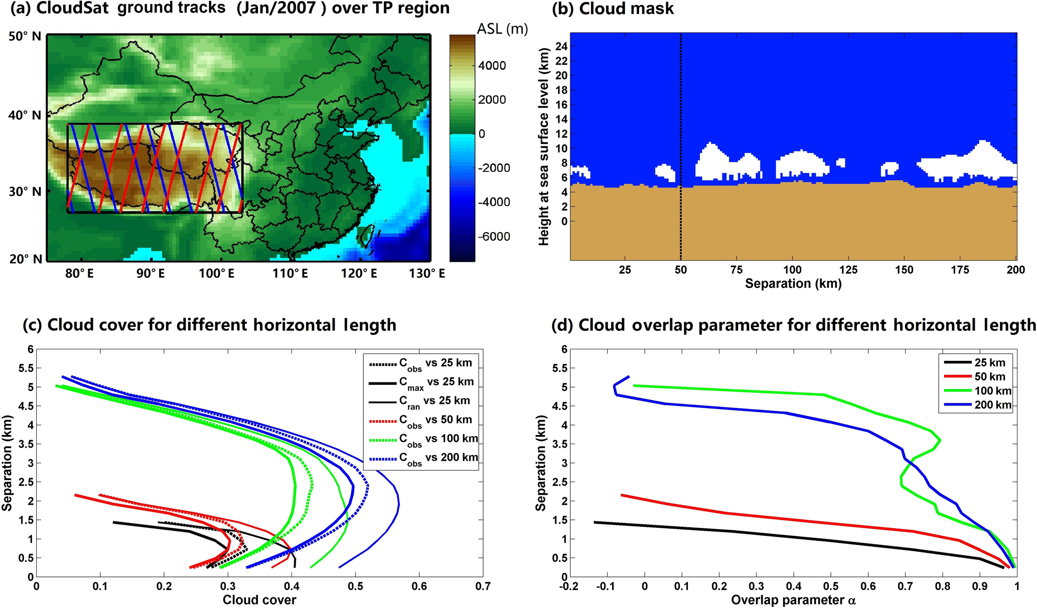
Figure 1(a) CloudSat overpass tracks (blue line: daytime; red line: nighttime) over the Tibetan Plateau (27–39∘ N; 78–103∘ E); (b) A sample of the CloudSat 2B-GEOPROF-LIDAR cloud mask product along the ground track of 200 km (white color: cloud fraction > 99 %; light blue: 0 < cloud fraction < 99 %; deep blue: clear sky; orange color: surface). (c) The observed and calculated segment-average cloud cover profiles based on maximum and random assumptions for different spatial scales and given cloud mask sample in (b). (d) The corresponding cloud overlap parameters of contiguous cloud layers for 25, 50, 100, and 200 km spatial scales, respectively. Note that the observations below 1 km over the TP surface have been removed.
To date, however, the related question of the cloud overlap over the TP region has received little attention due to the limited availability of observations. It is still an open question as to how the unique thermodynamic and dynamic environment over the TP affects cloud overlap there. The millimeter-wavelength cloud profiling radar (CPR) launched on CloudSat (Stephens et al., 2002) and the cloud-aerosol lidar with orthogonal polarization (CALIOP) (Winker et al., 2007) launched on CALIPSO (Cloud-Aerosol Lidar and Infrared Pathfinder Satellite Observation) provide an unprecedented opportunity to investigate vertical cloud overlaps on a global scale (e.g., Barker, 2008; Kato et al., 2010; Mace et al., 2009; Li et al., 2011a, b, 2015; Tompkins and Di Giuseppe, 2015). In the following study, we investigate the cloud overlap properties over the TP region and identify an empirical relationship between decorrelation length scale L and large-scale atmospheric dynamics by combining the cloud cover profile information from the 2B-GEOPROF-LIDAR dataset (Mace et al., 2009; Mace and Zhang, 2014) and the meteorological fields from the ERA-Interim reanalysis dataset (Dee et al., 2011). The parameterization of decorrelation length scale L will help to improve the simulation of total cloud cover and the calculation of radiative energy budget over the TP in the models. This paper is organized as follows. The datasets and methods used in this study are briefly described in Sect. 2. Section 3 outlines the monthly and zonal variations in the cloud overlap parameters over the TP region. The impacts of the atmospheric state and large-scale atmospheric dynamics on cloud overlap are presented in Sect. 4. The conclusions and discussion are given in Sect. 5.
Four years (2007–2010) of data from the CloudSat 2B-GEOPROF-LIDAR, ECMWF-AUX, and the daily 6 h ERA-Interim reanalysis are used to analyze the impacts of atmospheric states and dynamics on the cloud overlap over the TP (27–39∘ N; 78–103∘ E) region (Fig. 1a).
2.1 Satellite datasets
Radar signals can penetrate the optically thick cloud layers that attenuate lidar signals, but lidar signals may sense the optically thin hydrometeor layers that are below the detection threshold of radar signals. Thus, with the unique complementary capabilities of the CPR on CloudSat and CALIOP on CALIPSO, the 2B-GEOPROF-LIDAR dataset produces the most accurate description of the locations of the hydrometeor layers in the atmosphere on the global scale (Mace and Zhang, 2014). In this dataset, every CloudSat profile includes 125 height layers (e.g., vertical bin), and the Cloud Fraction parameter reports the fraction of the lidar volume within each radar vertical bin that contains hydrometeors (Mace et al., 2009; Mace and Zhang, 2014). Several previous studies have identified a cloudy atmospheric bin based on different thresholds of the lidar-identified cloud fraction, including a 99 % (Barker, 2008; Di Giuseppe and Tompkins, 2015) or a 50 % threshold (Haladay and Stephens, 2009; Verlinden et al., 2011). Here, a threshold of 99 % is used in our study. Due to the significant attenuation of lidar signals to the optically thick layers, this parameter fails to provide the Cloud Fraction for optically thick layers. Thus, we also use the radar information (i.e., cloud LayerBase and LayerTop fields) from the aforementioned dataset to construct the complete two-dimensional cloud mask (See Fig. 1b). It is worth noting that the 2B-GEOPROF-LIDAR dataset does not distinguish between cloud and precipitation; therefore, any bias in our results caused by precipitation cannot be removed in current analysis. Besides the 2B-GEOPROF-LIDAR dataset, the ECMWF-AUX dataset (Partain, 2004), which is an intermediate dataset consisting of the ancillary ECMWF state variables interpolated across each CloudSat CPR bin, is also used to provide the pressure and height information of each vertical bin in the cloud mask profile. The vertical and horizontal resolutions of these products are 240 m and 1.1 km, respectively. To avoid sunlight scattering contamination to lidar observation and to minimize surface contamination of the CPR, we only use the nighttime datasets above 1 km over the TP surface in the following analysis.
2.2 Meteorological reanalysis dataset
The 6-hourly ERA-Interim reanalysis with a grid resolution of 0.25∘ × 0.25∘ (Dee et al., 2011) is used to characterize the atmospheric thermodynamic and dynamic states over the TP. For each cloud mask profile in the 2B-GEOPROF-LIDAR, the vertical profiles of the zonal wind u, meridional wind v, relative humidity RH, specific humidity sh, and atmospheric temperature T closest to the cloud profile in both space and time are extracted and further interpolated vertically to match the vertical bins of the cloud mask profile. Following Di Giuseppe and Tompkins (2015), the u and v winds at every vertical bin are then projected onto the satellite overpass track, being averaged in the along-track direction for all profiles in the selected CloudSat data segment to derive the scene-average, along-track horizontal wind V. Here, we define the wind shear between the layers i and j, as follows:
where Vi and Vj are the horizontal winds at layers i and j, respectively, and Di,j is the layer separation distance. The derived wind shear will be used to calculate the cloud overlap parameter. For the CloudSat overpass track (Fig. 1a), Di Giuseppe and Tompkins (2015) indicated that the cross-track shear of the zonal wind u contributes little to the statistics of wind shear.
Similarly to the wind shear, we calculate the vertical gradient of the saturated equivalent potential temperature () between the same two layers to quantify the dependence of the cloud overlap on the degree of the conditional instability of the moist convection. Here,
where θ is the potential temperature, Lv is the latent heat of vaporization, rs is the saturation mixing ratio, Cp is the specific heat capacity at a constant pressure, and T is the atmospheric temperature. The smaller the , the more unstable the atmosphere. Furthermore, the scene-averaged vertical velocity at 500 hPa is also extracted from the ERA-Interim reanalysis to analyze the impact of vertical motion on cloud overlap. The positive values are for the updraft, and negative values are for the subsidence.
2.3 The overlap parameter and its dependence on the spatial scale
Previous studies have shown that the overlap parameter α and decorrelation length L are sensitive to the spatial scale of the general circulation models (GCMs) grid box (Hogan and Illingworth, 2000; Oreopoulos and Khairoutdinov, 2003; Oreopoulos and Norris, 2011; Pincus et al., 2005). For example, Hogan and Illingworth (2000) found that the cloud overlap parameter tends to increase with decreasing spatial and temporal resolutions (i.e., increasing vertical and horizontal grid scales) of GCMs.
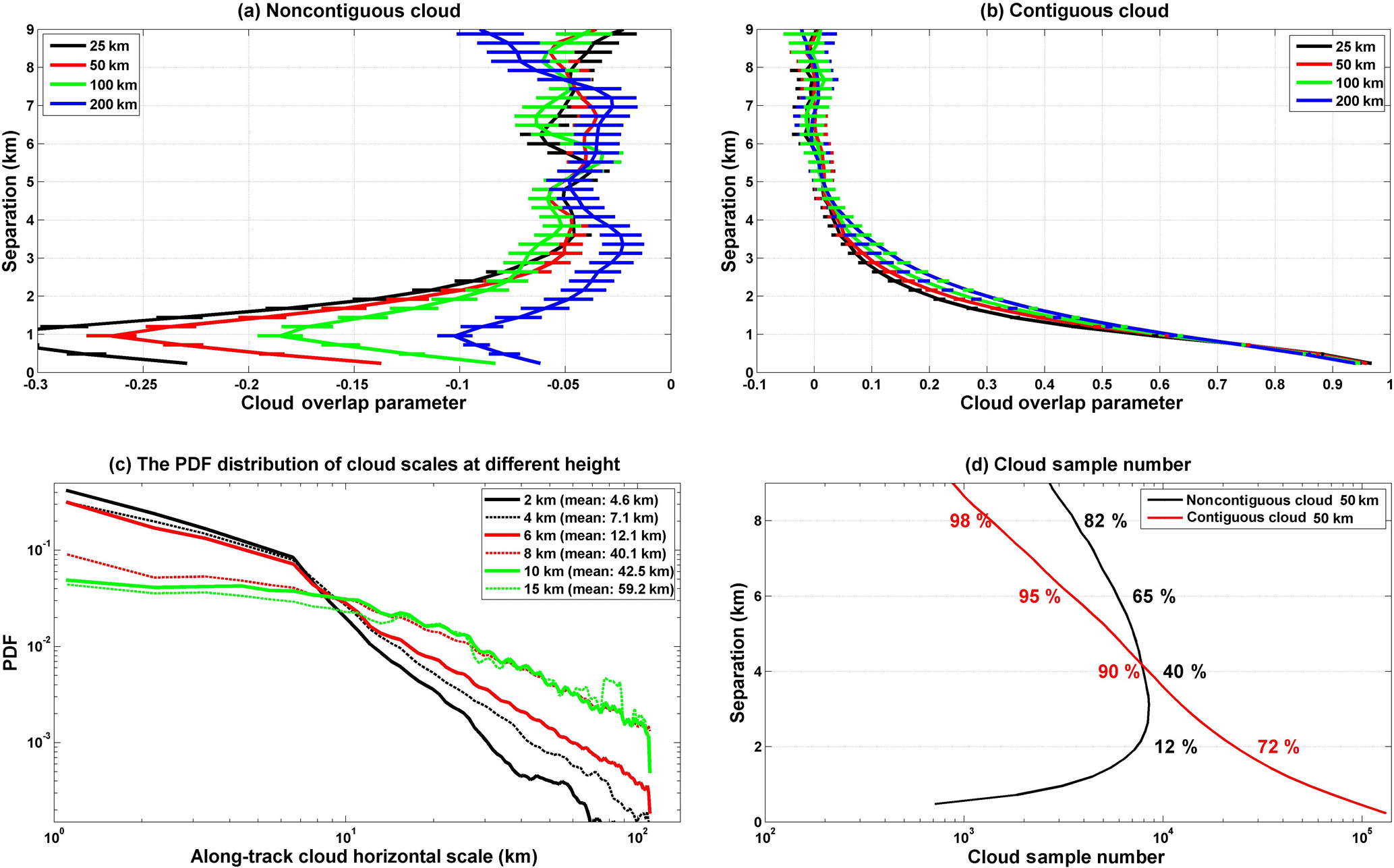
Figure 2The dependence of α on the layer separation and its sensitivity to the spatial scale for (a) noncontiguous and (b) contiguous cloud pairs; the horizontal bars correspond to means ± 3 standard errors, which represent the upper and lower endpoints of the 99 % confidence interval. (c) The probability distribution functions (PDFs) of the along-track horizontal scales of the cloud system at a different height over the TP region. (d) The variations in cloud sample number and the cumulative percentages with cloud layer separations for both noncontiguous and contiguous clouds at a given spatial scale of 50 km. The cumulative percentages represent the proportions of cloud sample below the corresponding layer separation to all samples.
To examine the dependence of the overlap parameter on the spatial scale, each CloudSat orbit over the TP region is divided into segments with different horizontal lengths including 25, 50, 100, and 200 km. Hereafter, this horizontal length is referred to as the effective spatial scale of the GCM's grid box. Figure 1b shows an example of cloud mask from the 2B-GEOPROF-LIDAR dataset over the TP region. This cloud mask includes eight, four, two, and one segments, which correspond to the horizontal resolution of 25, 50, 100, and 200 km, respectively. Given the threshold of 99 % for cloud fraction, the segment-average cloud cover profile of each segment is first derived. Here, it is important to emphasize that cloud fraction and cloud cover are different variables in our study. The Cloud fraction reports the fraction of lidar volumes in each radar vertical bin that contains hydrometeors and is used to identify a cloudy atmospheric bin based on the chosen threshold of 99 %. When averaging all cloud fraction profiles in the along-track direction for a given CloudSat data segment, we derive the segment-average cloud cover profile, which represents the percentage of clouds in a given spatial scale and certain height. Then, the vertical overlap between any two atmospheric layers in this profile is calculated if the cloud covers (Ci and Cj) of both layers exceed 0. Layers are analyzed in pairs and there is no “double-counting”. If cloud layer pairs have the same separation distance but different altitudes, they will be categorized as belonging to the same statistic group. Following Hogan and Illingworth (2000) and Di Giuseppe and Tompkins (2015), we consider the non-adjacent layers to be a contiguous cloud pair when all layers between them are classified as cloud layers. Otherwise, these layers are classified as a noncontiguous cloud pair (Hogan and Illingworth, 2000; Di Giuseppe and Tompkins, 2015).
Based on the definitions of different overlap assumptions and α in the introduction section, Fig. 1c and d show an example of the observed and calculated segment-average cloud cover profiles based on maximum and random assumptions, and corresponding overlap parameters of contiguous cloud pairs for the 25, 50, 100, and 200 km spatial scale in a given cloud mask sample (Fig. 1b). It is clear that the observed and calculated cloud covers and corresponding overlap parameters tend to increase as the spatial scale increases. In the meantime, the observed cloud covers tend to transform from the maximum to the random overlap assumption with increasing layer separations.
By collecting 4 years of cloud sample from the 2B-GEOPROF-LIDAR dataset, Fig. 2a and b further show the dependence of α on the layer separation and its sensitivity to the spatial scale for both noncontiguous and contiguous cloud layers. Many studies have used ground- and space-based radars to examine the validity of the random overlap assumption for vertically noncontiguous clouds (Hogan and Illingworth, 2000; Mace at al., 2002; Naud et al., 2008; Di Giuseppe and Tompkins, 2015). Figure 2a shows that the degree of cloud overlap of the noncontiguous clouds over the TP region is lower than the random overlap, especially when the layer separation is smaller than 2 km. Given the spatial scale of 50 km, almost all of the α values are negative and fall between −0.25 and −0.05. Thus, the total cloud cover would still slightly be underestimated for noncontiguous cloud pairs by using the random overlap assumption. Assuming a cloud layer separation of less than 9 km, α for noncontiguous cloud pairs increases as the spatial scale increases (e.g., from 25 to 200 km). For a contiguous cloud pair (Fig. 2b), α decreases from 0.95 to 0 with an increasing separation. In the meantime, a slight dependence of α on the spatial scale is also observed for contiguous cloud pairs when they are separated by a distance of about 1 to 4 km. This indicates that the maximum overlap is slightly more common for a larger horizontal domain, which is consistent with previous studies (Hogan and Illingworth, 2000; Oreopoulos and Khairoutdinov, 2003; Oreopoulos and Norris, 2011).
2.4 Selection of thresholds for cloud cover and spatial scale
Regarding the dependence of α on a spatial scale, Tompkins and Di Giuseppe (2015) theorized that some overcast or single cloud layers would be removed from the samples when the spatial scale is smaller than the cloud system scale, thus biasing α and its decorrelation length L. Given a spatial scale of 50 km, the ratio of the spatial scale to the cloud system scale decreases strongly from the equator to the poles because many of the frontal cloud systems of the middle and high latitudes are larger than the convective cloud systems over the tropics. Ultimately, the corresponding bias in α would increase with latitude. For these reasons, regional atmospheric models should account for the typical cloud system scale in their parameterization schemes when using a fixed horizontal resolution.
Figure 2c depicts the probability distribution functions (PDFs) of the horizontal scales of the along-track cloud systems at different heights over the TP region. Here, the horizontal scale of a cloud system at a given height along the CALIPSO/CloudSat track is determined by calculating the number of continuous cloud profiles (N) at a given height. Using a 1.1 km along-track resolution for the CPR measurements, the along-track scale (S) of a cloud system is S=N × 1.1 km (Zhang et al., 2014; Li et al., 2015). It is clear that the probability of a cloud system with a small-scale decreases with increasing height (Fig. 2c). The mean horizontal scale of 59.2 km for a cloud system at a height of 15 km is almost 12 times greater than that (i.e., 4.6 km) at a height of 2 km. For the TP region, we can see that the horizontal scales of cloud system below 10 km are smaller than the spatial scale of 50 km; thus, we apply the spatial scale of 50 km to perform the following analysis, although this scale would still result in significant errors in α at greater atmospheric heights (e.g., 15 km), where clouds have a larger horizontal scale.
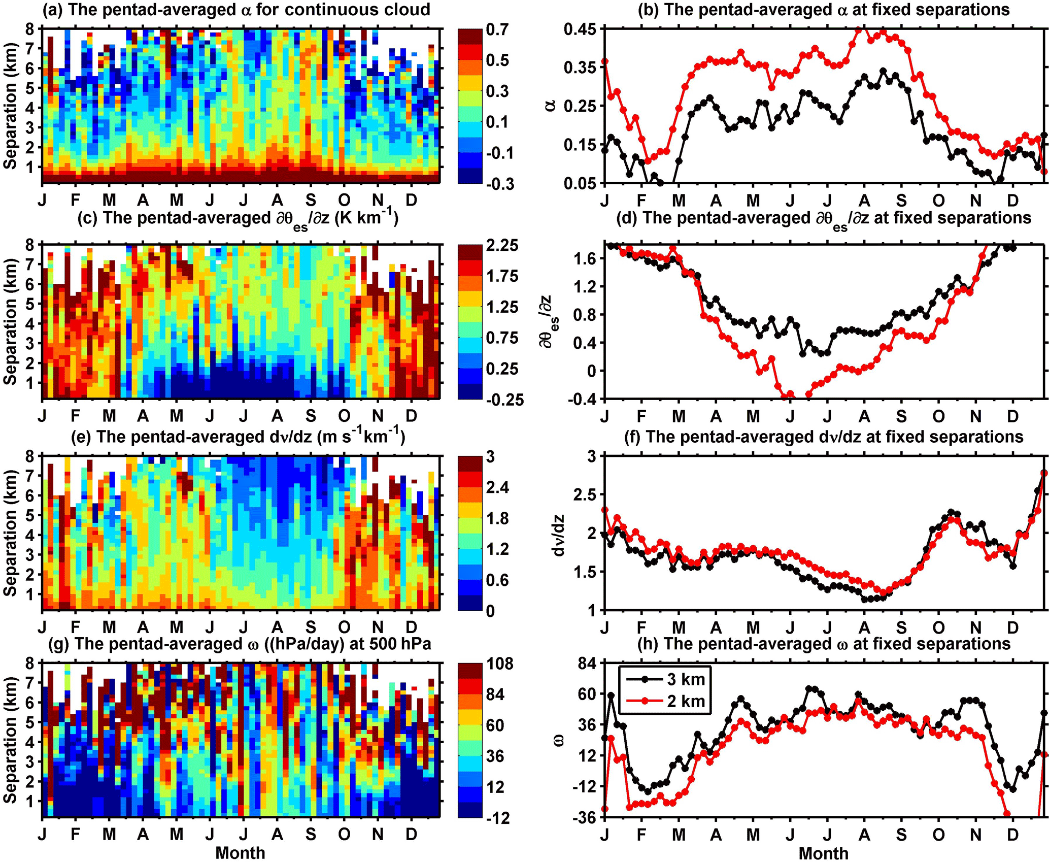
Figure 3The monthly variations in the pentad-averaged (a) cloud overlap parameter, α, (c) conditional instability to moist convection, (K km−1), (e) wind shear, dV∕dz (m s−1 km−1), and (g) vertical velocity ω (hPa day−1) at 500 hPa, for the contiguous cloud layers over the TP. The monthly variations in the pentad-averaged (b) α, (d) , (f) dV∕dz, and (h) ω for the contiguous clouds for the layer separation of 2 km (red) and 3 km (black).
In addition, to further reduce the sensitivity of α to the spatial scale caused by data truncation, we follow the study from Tompkins and Di Giuseppe (2015) and apply a simple data filter so that only atmospheric layers with segment-average cloud cover below a given threshold of 50 % are retained. As stated by Tompkins and Di Giuseppe (2015), data might still be truncated with this filter, but the sensitivity of the results to the spatial scale should largely be reduced. Here, we need to emphasize that the thresholds of 99 and 50 % used in our study correspond to the cloud fraction and cloud cover, respectively. After limiting the spatial scale (50 km) and upper limit of cloud cover (50 %), the number of available cloud layer pair samples is still at least 1 million, thus ensuring representative sampling. Figure 2d shows the variations in sample number and the cumulative percentage with cloud layer separation for both noncontiguous and contiguous clouds at a given spatial scale of 50 km. It shows that the cumulative proportion of cloud sample significantly increases with increasing layer separation. For the contiguous cloud, the cumulative percentage accounts for 90 % of all samples when layer separation is smaller than 4 km. Given the 1.1 km along-track resolution of the CPR measurements and a spatial scale of 50 km (that is, about 50 CloudSat profiles), each cloudy CloudSat profile has a cloud cover of about 2 % (Di Giuseppe and Tompkins, 2015).
Figure 3a shows the monthly variations in α for the contiguous cloud pairs based on pentad averages over the TP. In Fig. 3a, the maximum separation of contiguous cloud layers gradually increases from January (approximately 6 km) to August (beyond 8 km) and then gradually decreases, indicating that the cloud systems over the TP during summer are thicker than those clouds during other seasons due to frequent strong convective motions. When the cloud layer separation is less than 1 km, the overlap parameter α has little monthly variation and is always large (even beyond 0.7). However, the monthly variation in α becomes manifest when the layer separation is larger than 1 km. For a 2 km cloud separation, for example, α reaches its maximum of 0.45 in August and a minimum of 0.1 in February (see Fig. 3d). For a separation of 3 km, α is generally lower but has the similar monthly variation to those seen for a 2 km separation. The negative values of α in Fig. 3a show that even the random overlap assumption could underestimate the total cloud cover between two cloud layers with large separation during all seasons except summer. These cloud overlap features may be associated with the unique topographical forcing and corresponding thermodynamic and dynamic environment of the TP. In summer, the TP is usually considered an atmospheric heat source or “air pump” due to its higher surface temperature compared with surrounding regions at the same altitude (Wu et al., 2015). Additionally, humid and warm air intrudes from the South Asia monsoon into the lower atmosphere over the TP, which intensifies the atmospheric instability of moist convection when combined with the enhanced surface heating (Taniguchi and Koike, 2008). This process further promotes the transport of water vapor to high altitudes and favors the development of convective clouds. Indeed, satellite observations have indicated that cumulus prevails over the TP during the summer (Wang et al., 2014; Li and Zhang, 2016).
In view of the small horizontal scale of cumulus, a 50 km-spatial scale from CloudSat should not bias the α estimate too much in our study. However, previous studies have pointed out that precipitation may bias the cloud overlap statistics toward maximum overlap (Mace et al., 2009; Di Giuseppe and Tompkins, 2015), which is not accounted for in the present study. If we exclude the samples with precipitation from the analysis, the overlap parameter α would become smaller. The feature may be even more obvious during summer due to more frequent precipitation over the TP during this season (Yan et al., 2016). The seasonal variation in α is also found at different ground sites (Mace and Benson-Troth, 2002; Naud et al., 2008). For example, Oreopoulos and Norris (2011) indicated that cloud overlap tends to be more random in the winter and mostly maximum during the summer. In fact, these overlap properties are associated with the cloud system scale, which is dominated by the large-scale dynamical situation (Tompkins and Di Giuseppe, 2015).
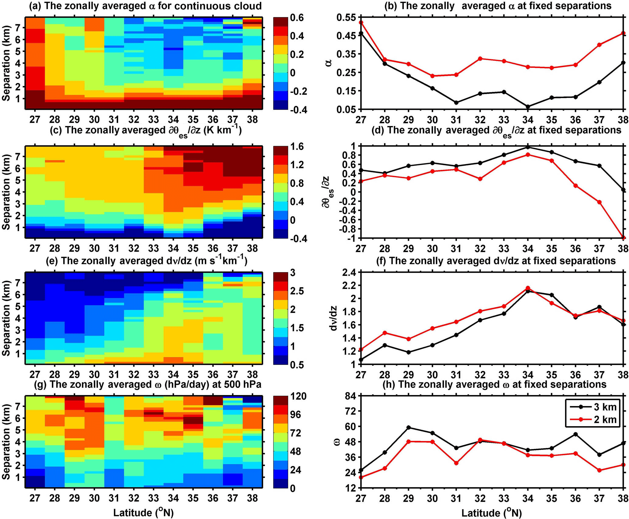
Figure 4The zonal variations in the (a) α, (c) (K km−1), (e) dV∕dz (m s−1 km−1), and (g) ω (hPa day−1) for the contiguous cloud layers over the TP. The zonal variations in the (b) α, (d) , (f) dV∕dz, and (h) ω for the contiguous cloud layers for the layer separation of 2 km (red) and 3 km (black).
Figure 3b and c show the monthly variations in pentad-averaged conditional instability of moist convection () and wind shear (dV∕dz) for the contiguous cloud pairs over the TP, respectively. Both and dV∕dz exhibit clear monthly variations for all cloud-layer separations. The atmospheric stability and wind shear gradually decrease from January to August and then steadily increase (see Fig. 3c, d, e, and f). From Fig. 3c, we can see that the adjacent atmospheric layers during May to September tend to be more unstable and have weak wind shear. These atmospheric states favor the development of clouds and result in maximum overlap between cloud layers. During other months (e.g., December), clouds also tend to follow the maximum overlap more although adjacent atmospheric layers are stable with large and dV∕dz. It might be the case that vertical velocities are large because of extratropical cyclones or other sources of baroclinic instability. When the layer separation increases, atmospheric layers become more stable and then favor random overlap, especially during the summer season. These results verify that a more unstable atmosphere tends to favor a maximum overlap of cloud layers over a random one, as shown in previous studies (Mace and Benson-Troth, 2002; Naud et al., 2008). Note that Fig. 3d and f might reveal an inconsistency between the wind shear and atmospheric stability. For example, we can see that the wind shear for a 2 km layer distance is greater than that for a 3 km distance, but the atmosphere is also more unstable. This inconsistency is probably because two cloud layers with the same separation but occurring at different altitudes are sorted into the same statistical group. Or it is also possible that other large-scale forcings might influence the overlap. In addition, we find the monthly variations in pentad-averaged vertical velocity (ω) at 500 hPa (see Fig. 3g and h) are also consistent with the monthly cycle of α. It means that vigorous ascent tends to favor maximum overlap. This result agrees well with the previous studies (Naud et al., 2008).

Figure 5The sensitivities of median overlap parameter α to the (a) wind shear, (b) instability, and (c) vertical velocity at 500 hPa at a given upper limit of cloud cover (50 %) and spatial scale (50 km) for the contiguous cloud layers. The horizontal bars correspond to means ± 3 standard errors, which represent the upper and lower endpoints of the 99 % confidence interval.
Figure 4 shows the zonal variations in α, , dV∕dz, and ω over the TP. Figure 4a and b indicate that α is larger in the south part of the TP and smaller in the north. This is mainly because atmospheric instability in the southern part of the TP enhances convective activity (Fujinami and Yasunari, 2001). Due to the weakening of the monsoon and the blocking by topography, less water vapor may reach the northern part of the TP, and thus fewer clouds form there (You et al., 2014). Compared with the southern TP, the stability and wind shear are both larger over the northern part, especially for those cloud layers with large separation (e.g., > 2 km). These meteorological conditions will result in more frequent negative α, indicating that the random overlap assumption used in models would underestimate the total cloud cover and thus bias the surface radiation over these regions (see Fig. 4a). The most significant warming occurring over the northern part of the TP has been attributed to pronounced stratospheric ozone depletion (e.g., Guo and Wang, 2012). However, a more recent study indicates that the accelerated warming trend over the Tibetan Plateau may be due to the rapid cloud cover increases at nighttime over the northern Tibetan Plateau and the sunshine duration increase in the daytime over the southern Tibetan Plateau (Duan and Xiao, 2015). Therefore, an accurate representation of cloud overlap and its relations to atmospheric thermodynamic and dynamic conditions in models are critically important to the understanding of rapid warming over the TP. Although it is still difficult for models to capture the cloud overlap properties, especially for those cloud layers with large separation over the north TP, our results confirm that the α is well related to wind shear and instability. However, the zonal variation in α is inconsistent with the variation in vertical velocity (see Fig. 4g and h).
To facilitate the parameterization of α for cases of contiguous clouds, we further investigate the sensitivity of α to the different meteorological conditions. Here, each meteorological factor over the TP region is grouped into one of four bins as follows. The four bins for are > 5 K km−1, 2.5 < < 5 K km−1, 0 < < 2.5 K km−1, < 0 K km−1. For wind shear, the four bins are dV∕dz < 0.5 m s−1 km−1, 0.5 < m s−1 km−1, 2 < dV∕dz < 3.5 m s−1 km−1, and dV∕dz > 3.5 m s−1 km−1. For vertical velocity, the four bins are ω < −40 hPa day−1, −40 < ω < 0 hPa day−1, 0 < ω < 40 hPa day−1, and ω > 40 hPa day−1. These groupings ensure that a statistically representative number of samples fall within each bin (i.e., at least 1 000 000 samples per bin). In addition, Li et al. (2015) indicated that the overlap properties between different cloud types are also important for the Earth's climate system. Although this study does not include the information on cloud type, the dependence of α on meteorological parameters found in our analysis actually demonstrates the effects of cloud types on the α because different combinations of cloud type with the same layer separation possibly occur in distinct wind shear and stability conditions.
Table 1Parameterizations of decorrelation scale length L from the exponential fit as a function of atmospheric stability , wind shear dV∕dz or latitude Φ.
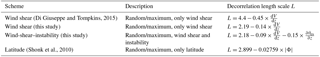
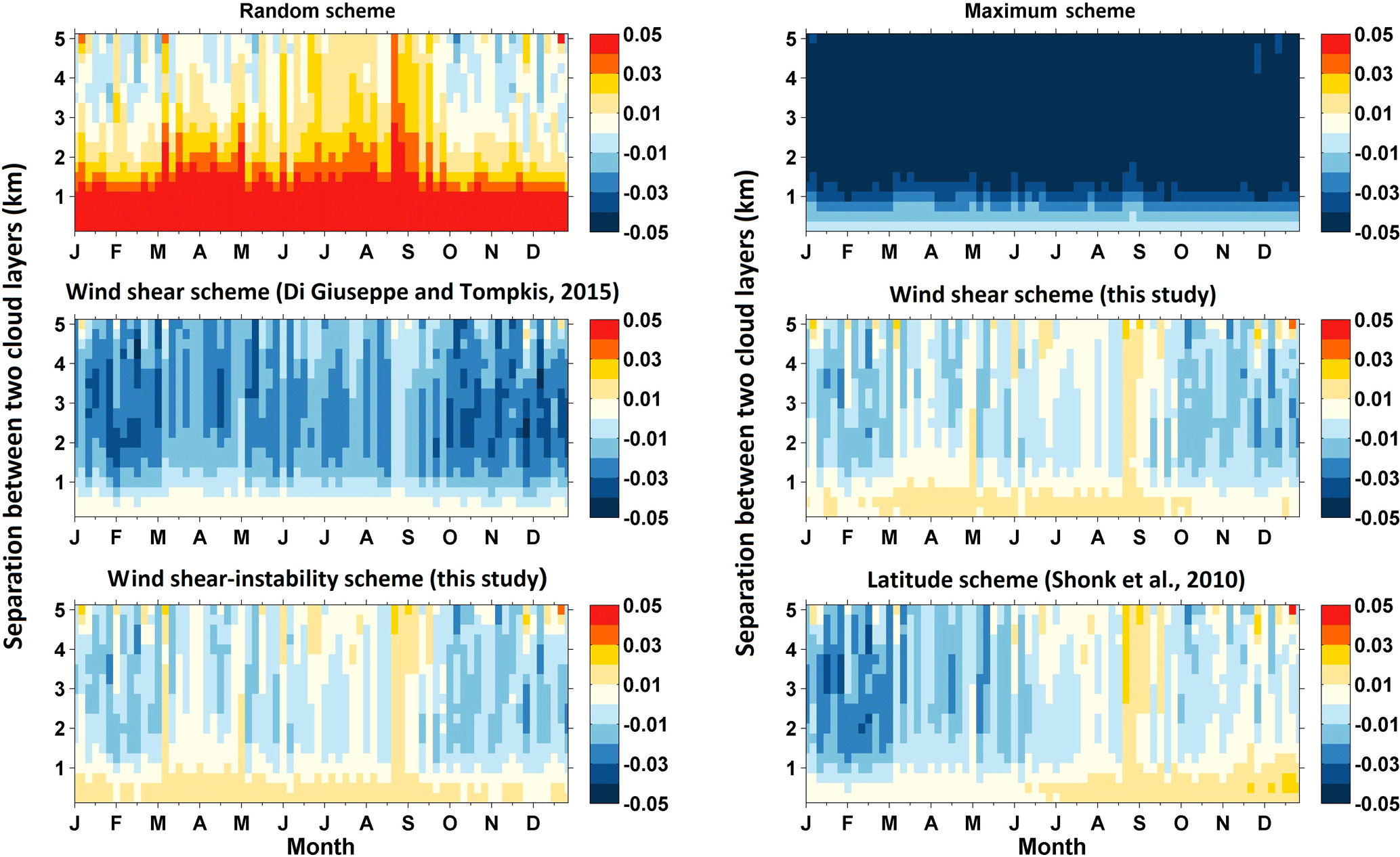
Figure 6The monthly differences in total cloud cover (unitless) between calculation and observation for different schemes (see Table 1) and their dependence on the layer separation.
Figure 5 illustrates the sensitivity of α to wind shear, instability, and vertical velocity at a given upper limit of cloud cover (50 %) and spatial scale (50 km) for the contiguous clouds. Since the cloud samples with layer separation below 3.5 km account for 90 % of all samples for contiguous clouds, we only present the results for layer distances smaller than 3.5 km. Naud et al. (2008) tested the sensitivity of α to wind shear at three sites and found that wind shear slightly affects α when the layer distance is larger than 2 km. In a recent study, Di Giuseppe and Tompkins (2015) demonstrated the important effect of wind shear on the global cloud overlap by using a combination of the CloudSat-CALIPSO cloud data and the ECMWF reanalysis dataset. Our results along with previous studies suggest that the cloud overlap strongly depends on atmospheric conditions, but their relationship displays some variability, in particular spatially and seasonally. The effect of the atmospheric stability on cloud overlap may be more important over convective regions (e.g., the intertropical convergence zone and the TP during the summer season), while the effect of wind shear may be dominant over the midlatitudes. Besides the wind shear and instability, some studies also tested the sensitivity of the overlap parameter to the large-scale vertical velocity. For example, Naud et al. (2008) indicated that vertical velocities in the tropics are not captured in the reanalysis dataset when convection occurs; thus, they only discussed the impact of vertical velocity on the cloud overlap parameter over the midlatitudes and found that vigorous ascent tends to favor maximum overlap. Fig. 5c shows that vertical velocity at 500 hPa has some effect on the cloud overlap parameter. However, by combining the effects of wind shear, instability, and vertical velocity into parameterization of decorrelation length scale L, we find that this scheme is not superior to a scheme which only includes the wind shear and instability.
Here, we derive the decorrelation length scale L values (km) from the least squares exponential fit to the original α curve at given wind shear and instability bin. Then, we further parameterize L as a function of wind shear or both wind shear and atmospheric instability based on a (multiple) linear regression. The regression formula of L can be written as
Here, Lα, Lα1, b1, b2, and c1 are the fitting parameters. Table 1 lists several parameterization schemes for the decorrelation length scale L. The scheme with wind shear from Di Giuseppe and Tompkins (2015) using the global CloudSat-CALIPSO cloud data and ECMWF reanalysis dataset is shown for comparison. Di Giuseppe and Tompkins (2015) discussed the uncertainties from fitting methods and the calculation of wind shear. Related to the observational orbit, the impact of cross-track wind shear is neglected in our study, which would exclude many large wind shears associated with jet structures (Di Giuseppe and Tompkins, 2015). The parameterization scheme of Shonk et al. (2010) is also shown in Table 1, which is an empirical linear relationship between L and latitude based on CloudSat and CALIPSO data. Our parameterization schemes in terms of wind shear or both wind shear and instability are given in Table 1. Note that the R-squared values (R2) for our wind shear and wind-shear–instability schemes are 0.88 and 0.96, respectively.

Figure 7The zonal differences in total cloud cover (unitless) between calculation and observation for different schemes (see Table 1) and their dependence on the layer separation.
After deriving the regression formula of decorrelation length scale L, we reapply it to all contiguous cloud samples and retrieve the L and corresponding α based on the formula and dynamical conditions. Finally, the retrieved overlap parameter α is used to calculate the total cloud cover between any two cloud layers by using Eq. (1) and definitions of random and maximum overlap assumptions. Figure 6 presents the monthly difference between calculated and observed cloud covers using various overlap parameterization schemes. It is seen that the maximum and random overlap assumptions result in large cloud cover biases, especially for layer separations greater than 1 km for maximum overlap and less than 2 km for random overlap where the bias exceeds 5 %. Compared with random and maximum assumptions, the differences between total cloud cover caused by other schemes are small and range from −3 to 3 %. In addition, the wind shear scheme and the wind-shear–instability scheme from the present study overall show less biases than other schemes. However, several points should be further noted. First, the wind shear scheme from Di Giuseppe and Tompkins (2015) significantly underestimates the cloud cover for layer separations above 1 km (e.g., by up to 3 %). This large bias may be because it is based on the global CloudSat-CALIPSO measurements and ECMWF reanalysis dataset for a short period (January–July 2008); as such, some obvious regional or seasonal cloud overlap properties are easily obscured by global averaging. Furthermore, the role of atmospheric stability is not considered in this scheme. However, the scheme from Di Giuseppe and Tompkins (2015) shows little bias for layer separations below 1 km. This is because this scheme retrieves much larger L and overlap parameter values than other schemes. An interesting finding is that the latitude scheme from Shonk et al. (2010) leads to a bias comparable to new schemes from this study. The bias is even smaller for the latitude scheme when the layer separation is below 1 km. In fact, Fig. 5 has demonstrated that the sensitivity of α to wind shear and instability is rather weak when cloud layers are very close. Our wind-shear–instability scheme further combines the impact of atmospheric instability and has a relatively lower bias at large layer separations with higher R-squared values (R2=0.96).
Figure 7 shows the zonal difference between calculated and observed cloud covers for the aforementioned schemes. The differences between cloud cover caused by different overlap schemes are obvious. Similar to Fig. 6, the maximum and random overlap assumptions still result in the most prominent cloud cover biases (exceeding ±5 %) at most of the layer separations. Compared with our wind shear scheme and wind-shear–instability schemes, the scheme from Di Giuseppe and Tompkins (2015) and latitude scheme from Shonk et al. (2010) cause a clear underestimation of total cloud cover when cloud layer separations exceed 1 km, especially for scheme from Di Giuseppe and Tompkins (2015) (bias reaching −3 %). Only if cloud layer separations are smaller than 1 km, do these two schemes produce a better cloud cover simulation than our schemes. In summary, these results indicate that a new parameterization (that is, our wind-shear–instability scheme) of decorrelation length scale L, which includes the effects of both wind shear and atmospheric stability on cloud overlap, may improve the simulation of total cloud cover over the TP.
Clouds strongly modulate the Earth's radiative energy budget via changes in their macro- and microphysical properties (e.g., Hartmann et al., 1992; Fu and Liou, 1993; Fu et al., 2002; Kawamoto and Suzuki, 2012; Yan et al., 2014; Wang et al., 2010). Many studies have shown that annual and seasonal changes in total cloud cover are responsible for the rapid climate warming over the Tibetan Plateau in the past 3 decades (e.g., Yang et al., 2012; You et al., 2014; Duan and Xiao, 2015).
To accurately simulate the total cloud cover and its impact on the radiative energy budget, climate models need to reliably represent the cloud vertical overlap, which has received less attention than necessary because of the limited availability of regional cloud observations. In view of the passive sensors only providing limited information about the cloud overlap (Chang and Li, 2005a, b; Huang, 2006; Huang et al., 2005, 2006) and the vertically resolved advantage of active sensors (Ge et al., 2017, 2018; Zhao et al., 2016, 2017), this study utilizes the 4 years (2007–2010) of data from the CloudSat cloud product and collocated ERA-Interim reanalysis data to analyze the cloud overlaps over the Tibetan Plateau and to build an empirical relationship between cloud overlap properties and large-scale atmospheric dynamics. It is confirmed that the contiguous cloud layers tend to have maximum overlap at small separation but gradually become randomly overlapped with an increase in the layer separation. Focusing on the contiguous cloud layers, we evaluate the effects of the meteorological conditions on the cloud overlap. It is found that the unstable atmospheric stratification with a weak wind shear over the TP would tend to favor maximum overlap, agreeing well with previous studies. We parameterize the decorrelation length scale L, which is used to characterize the transition from the maximum to random overlap assumption, as a function of the wind shear and atmospheric stability. Compared with other parameterizations, this new scheme improves the prediction of total cloud cover over the TP when cloud layer separations are greater than 1 km. Although the scheme derived in our study focuses only on the TP, our results suggest that the parameterization of the decorrelation length scale L by considering multiple thermodynamic and dynamic factors and microphysical effects (e.g., precipitation) has the potential to improve the model-simulated total cloud covers.
In a recent study, Di Giuseppe and Tompkins (2015) applied the wind-shear-dependent decorrelation length scale in the ECMWF Integrated Forecasting System. They found that the impact of wind-shear-dependent parameterization on radiative budget calculation is comparable in magnitude to that of the latitude-dependent scheme of Shonk et al. (2010). Our results also show that the latitude-dependent scheme has a similar bias of cloud cover to the new scheme developed in this study. Although our results cannot identify which of the schemes is superior, the scheme based on the meteorological factors has some potential advantages. For example, the cloud overlap parameter is significantly controlled by atmospheric thermodynamic and dynamical conditions; therefore, the long-term variations in meteorological factors are bound to affect the trend of cloud overlap and corresponding calculations of total cloud cover and radiation budget. Indeed, a recent study has shown that rapid warming and an increase in atmospheric instability over the TP leads to more frequent deep clouds, which are responsible for the reduction in solar radiation over the TP (Yang et al., 2012). By using surface observations over 71 stations, some studies verified that annual and seasonal total cloud covers have declined during 1961–2005 (Duan and Wu, 2006; You et al., 2014). However, whether such variations in total cloud cover are linked with the changes in the degree of cloud overlap over the TP is still unclear. Thus, more efforts are needed to evaluate the impact of cloud overlap on the total cloud cover variations over sensitive areas of climatic change (e.g., the Tibetan Plateau and the Arctic).
The CloudSat datasets are available from the CloudSat website: (http://www.cloudsat.cira.colostate.edu/order-data, CloudSat dataset, 2018). The ERA-Interim reanalysis daily 6 h products are downloaded from the ERA-Interim website: http://www.ecmwf.int/en/research/climate-reanalysis/era-interim (ERA-Interim, 2018).
The authors declare that they have no conflict of interest.
This research was jointly supported by the key Program of the National
Natural Science Foundation of China (41430425), the Foundation for Innovative
Research Groups of the National Science Foundation of China (grant no.
41521004), National Science Foundation of China (grant nos. 41575015 and
41575143), and the China 111 project (grant no. B13045). We would like to
thank the CALIPSO, CloudSat, and ERA-Interim science teams for providing
excellent and accessible data products that made this study
possible.
Edited by: Amanda
Maycock
Reviewed by: three anonymous referees
Barker, H. W.: Overlap of fractional cloud for radiation calculations in GCMs: A global analysis using CloudSat and CALIPSO data, J. Geophys. Res., 113, 762–770, 2008.
Barker, H. W. and Fu, Q.: Assessment and optimization of the Gamma-weighted two-stream approximation, J. Atmos. Sci., 57, 1181–1188, 2000.
Barker, H. W., Stephens, G. L., and Fu, Q.: The sensitivity of domain-averaged solar fluxes to assumptions about cloud geometry, Q. J. Roy. Meteor. Soc., 125, 2127–2152, 1999.
Chang, F. L. and Li, Z.: A New Method for Detection of Cirrus Overlapping Water Clouds and Determination of Their Optical Properties, J. Atmos. Sci., 62, 3993–4009, 2005a.
Chang, F. L. and Li, Z.: A near global climatology of single-layer and overlapped clouds and their optical properties retrieved from TERRA/MODIS data using a new algorithm, J. Climate, 18, 4752–4771, 2005b.
Chen, B. and Liu, X.: Seasonal migration of cirrus clouds over the Asian Monsoon regions and the Tibetan Plateau measured from MODIS/Terra, Geophys. Res. Lett., 32, 67–106, 2005.
Chen, T., Rossow, W. B., and Zhang, Y.: Radiative Effects of Cloud-Type Variations, J. Climate, 13, 264–286, 2000.
Cheng, G. and Wu, T.: Responses of permafrost to climate change and their environmental significance, Qinghai–Tibet Plateau, J. Geophys. Res., 112, F02S03, https://doi.org/10.1029/2006JF000631, 2007.
CloudSat dataset: CloudSat 2B-GEOPROF-LIDAR and ECMWF-AUX products, available at: http://www.cloudsat.cira.colostate.edu/order-data, last access: 23 May 2018.
Dee, D. P., Uppala, S. M., Simmons, A. J., Berrisford, P., Poli, P., Kobayashi, S., Andrae, U., Balmaseda, M., A. Balsamo, G., Bauer, P., Bechtold, P., Beljaars, A. C. M., Van De Berg, L., Bidlot, J., Bormann, N., Delsol, C., Dragani, R., Fuentes, M., Geer, A., J. Haimberger, L., Healy, S. B., Hersbach, H., Hólm, E. V., Isaksen, L., Kållberg, P., Köhler, M., Matricardi, M., McNally, A. P., Monge-Sanz, B. M., Morcrette,J. J., Park, B. K., Peubey, C., De Rosnay, P., Tavolato, C., Thépaut, J. N., and Vitart, F.: The ERA-Interim reanalysis: configuration and performance of the data assimilation system, Q. J. Roy. Meteor. Soc., 137, 553–597, 2011.
Di Giuseppe, F. and Tompkins, A. M.: Generalizing Cloud Overlap Treatment to Include the Effect of Wind Shear, J. Atmos. Sci., 72, 2865–2876, 2015.
Duan, A. M. and Wu, G. X.: Role of the Tibetan Plateau thermal forcing in the summer climate patterns over subtropical Asia, Clim. Dynam., 24, 793–807, 2005.
Duan, A. and Wu, G.: Change of cloud amount and the climate warming on the Tibetan Plateau, Geophys. Res. Lett., 33, 395–403, 2006.
Duan, A. and Xiao, Z.: Does the climate warming hiatus exist over the Tibetan Plateau?, Sci. Rep.-UK, 5, 13711, https://doi.org/10.1038/srep13711, 2015.
ERA-Interim: ERA-Interim reanalysis daily 6 h products, available at: http://www.ecmwf.int/en/research/climate-reanalysis/era-interim, last access: 23 May 2018.
Fu, Q. and Liou, K. N.: Parameterization of the radiative properties of cirrus clouds, J. Atmos. Sci., 50, 2008–2025, 1993.
Fu, Q., Cribb, M. C., Barker, H. W., Krueger, S. K., and Grossman, A.: Cloud geometry effects on atmospheric solar absorption, J. Atmos. Sci., 57, 1156–1168, 2000.
Fu, Q., Baker, M., and Hartmann, D. L.: Tropical cirrus and water vapor: an effective Earth infrared iris feedback?, Atmos. Chem. Phys., 2, 31–37, https://doi.org/10.5194/acp-2-31-2002, 2002.
Fujinami, H. and Yasunari, T.: The seasonal and intraseasonal variability of diurnal cloud activity over the Tibetan Plateau, J. Meteorol. Soc. Jpn., 79, 1207–1227, 2001.
Ge, J., Zhu, Z., Zheng, C., Xie, H., Zhou, T., Huang, J., and Fu, Q.: An improved hydrometeor detection method for millimeter-wavelength cloud radar, Atmos. Chem. Phys., 17, 9035–9047, https://doi.org/10.5194/acp-17-9035-2017, 2017.
Ge, J., Zheng C., Xie, H., Xin Y., Huang J., and Fu, Q.: Mid-latitude Cirrus Cloud at the SACOL site: Macrophysical Properties and Large-Scale Atmospheric State, J. Geophys. Res., 123, 2256–2271, https://doi.org/10.1002/2017JD027724, 2018.
Geleyn, J. F. and Hollingsworth, A.: An economical analytical method for the computation of the interaction between scattering and line absorption of radiation, Contrib. Atmos. Phys., 52, 1–16, 1979.
Guo, D. and Wang, H.: The significant climate warming in the northern Tibetan Plateau and its possible causes, Int. J. Climatol., 32, 1775–1781, https://doi.org/10.1002/joc.2388, 2012.
Haladay, T. and Stephens, G.: Characteristics of tropical thin cirrus clouds deduced from joint CloudSat and CALIPSO observations, J. Geophys. Res., 114, D00A25–D00A37, 2009.
Hartmann, D. L., Ockert-Bell, M. E., and Michelsen, M. L.: The effect of cloud type on Earth's energy balance: Global analysis, J. Climate, 5, 1281–1304, 1992.
Hogan, R. J. and Illingworth, A. J.: Deriving cloud overlap statistics from radar, Q. J. Roy. Meteor. Soc., 126, 2903–2909, 2000.
Huang, J. P.: Analysis of ice water path retrieval errors over tropical ocean, Adv. Atmos. Sci., 23, 165–180, 2006.
Huang, J. P., Minnis, P., and Lin, B.: Advanced retrievals of multilayered cloud properties using multispectral measurements, J. Geophys. Res., 110, D15S18, https://doi.org/10.1029/2004JD005101, 2005.
Huang, J. P., Minnis, P., and Lin, B.: Determination of ice water path in ice- over-water cloud systems using combined MODIS and AMSR-E measurements, Geophys. Res. Lett., 33, L21801, https://doi.org/10.1029/2006GL027038, 2006.
Jing, X., Zhang, H., Peng, J., Li, J., and Barker, H. W.: Cloud overlapping parameter obtained from CloudSat/CALIPSO dataset and its application in AGCM with McICA scheme, Atmos. Res., 170, 52–65, 2016.
Kang, S., Xu, Y., You, Q., Flügel, W. A., Pepin, N., and Yao, T.: Review of climate and cryospheric change in the Tibetan Plateau, Environ. Res. Lett., 5, 015101, https://doi.org/10.1088/1748-9326/5/1/015101, 2010.
Kato, S., Sun-Mack, S., Miller, W. F., Rose, F. G., Chen, Y., Minnis, P., and Wielicki, B. A.: Relationships among cloud occurrence frequency, overlap, and effective thickness derived from CALIPSO and CloudSat merged cloud vertical profiles, J. Geophys. Res., 115, 1–28, 2010.
Kawamoto, K. and Suzuki, K.: Microphysical transition in water clouds Over the Amazon and China derived from spaceborne radar and Radiometer data, J. Geophys. Res., 117, D05212, https://doi.org/10.1029/2011JD016412, 2012.
Li, J., Hu, Y., Huang, J., Stamnes, K., Yi, Y., and Stamnes, S.: A new method for retrieval of the extinction coefficient of water clouds by using the tail of the CALIOP signal, Atmos. Chem. Phys., 11, 2903–2916, https://doi.org/10.5194/acp-11-2903-2011, 2011a.
Li, J., Yi, Y., Minnis, P., Huang, J., Yan, H., Ma, Y., Wang, W., and Ayers, K.: Radiative effect differences between multi-layered and single-layer clouds derived from CERES, CALIPSO, and CloudSat data, J. Quant. Spectrosc. Ra., 112, 361–375, 2011b.
Li, J., Huang, J., Stamnes, K., Wang, T., Lv, Q., and Jin, H.: A global survey of cloud overlap based on CALIPSO and CloudSat measurements, Atmos. Chem. Phys., 15, 519–536, https://doi.org/10.5194/acp-15-519-2015, 2015.
Li, Y., Liu, X., and Chen B.: Cloud type climatology over the Tibetan Plateau: A comparison of ISCCP and MODIS/TERRA measurements with surface observations, Geophys. Res. Lett., 33, L17716, https://doi.org/10.1029/2006GL026890, 2006.
Li, Y. Y. and Zhang, M.: Cumulus over the Tibetan Plateau in the summer based on CloudSat–CALIPSO data, J. Climate, 29, 1219–1230, https://doi.org/10.1175/JCLI-D-15-0492.1, 2016.
Mace, G. G. and Benson-Troth, S.: Cloud-Layer Overlap Characteristics Derived from Long-Term Cloud Radar Data, J. Climate, 15, 2505–2515, 2002.
Mace, G. G. and Zhang, Q.: The CloudSat radar-lidar geometrical profile product (RL-GeoProf): Updates, improvements, and selected results, J. Geophys. Res., 119, 9441–9462, https://doi.org/10.1002/2013JD021374, 2014.
Mace, G. G., Zhang, Q., Vaughan, M., Marchand, R., Stephens, G., Trepte, C., and Winker, D.: A description of hydrometeor layer occurrence statistics derived from the first year of merged CloudSat and CALIPSO data, J. Geophys. Res., 114, D00A26, https://doi.org/10.1029/2007JD009755, 2009.
Morcrette, J. J. and Fouquart, Y.: The Overlapping of Cloud Layers in Shortwave Radiation Parameterizations, J. Atmos. Sci., 43, 321–328, 1986.
Morcrette, J. J. and Jakob, C.: The response of the ECMWF model to changes in the cloud overlap assumption, Mon. Wea. Rev., 128, 1707–1732, 2000.
Naud, C. M., Del Genio, A., Mace, G. G., Benson, S., Clothiaux, E. E., and Kollias, P.: Impact of dynamics and atmospheric state on cloud vertical overlap, J. Climate, 21, 1758–1770, 2008.
Oreopoulos, L. and Norris, P. M.: An analysis of cloud overlap at a midlatitude atmospheric observation facility, Atmos. Chem. Phys., 11, 5557–5567, https://doi.org/10.5194/acp-11-5557-2011, 2011.
Oreopoulos, L. and Khairoutdinov, M.: Overlap properties of clouds generated by a cloud-resolving model, J. Geophys. Res., 108, 4479, https://doi.org/10.1029/2002JD003329, 2003.
Partain, P.: Cloudsat ECMWF-AUX auxiliary data process description and interface control document, Coop. Inst. for Res. in the Atmos., Colo. State Univ., Fort Collins, 2004.
Pincus, R., Hannay, C., Klein, S. A., Xu, K. M., and Hemler, R.: Overlap assumptions for assumed probability distribution function cloud schemes in large-scale models, J. Geophys. Res., 110, D15S09, https://doi.org/10.1029/2004JD005100, 2005.
Shonk, J. K., Hogan, R. J., Edwards, J. M., and Mace, G. G.: Effect of improving representation of horizontal and vertical cloud structure on the Earth's global radiation budget. Part I: Review and parametrization, Q. J. Roy. Meteor. Soc., 136, 1191–1204, 2010.
Shonk, J. K. P., Hogan, R. J., and Manners, J.: Impact of improved representation of horizontal and vertical cloud structure in a climate model, Clim. Dynam., 38, 2365–2376, 2014.
Stephens, G. L., Vane, D. G., Boain, R. J., Mace, G. G., Sassen, K., Wang, Z., Illingworth, A. J., O'Connor, E. J., Rossow, W. B., Durden, S. L., Miller, S. D., Austin, R. T., Benedetti, A., Mitrescu, C., and CloudSat Science Team.: The CloudSat mission and the A-Train, A new dimension of space-based observations of clouds and precipitation, B. Am. Meteorol. Soc., 83, 1771–1790, 2002.
Taniguchi, K. and Koike, T.: Seasonal variation of cloud activity and atmospheric profiles over the eastern part of the Tibetan Plateau, J. Geophys. Res., 113, 523–531, 2008.
Tompkins, A. and Giuseppe, F. D.: An interpretation of cloud overlap statistics, J. Atmos. Sci., 72, 2877–2889, 2015.
Verlinden, K. L., Thompson, D. W. J., and Stephens, G. L.: The Three-Dimensional Distribution of Clouds over the Southern Hemisphere High Latitudes, J. Climate, 24, 5799–5811, 2011.
Wang, B., Bao, Q., Hoskins, B., Wu, G., and Liu, Y.: Tibetan Plateau warming and precipitation changes in East Asia, Geophys. Res. Lett., 35, L14702, https://doi.org/10.1029/2008GL034330, 2008.
Wang, M. Y., Gu, J., Yang, R., Zeng, L., and Wang, S.: Comparison of cloud type and frequency over China from surface, FY-2E, and CloudSat observations, in: Remote Sensing of the Atmosphere, Clouds, and Precipitation, edited by: Im, E., Yang, S., and Zhang, P., International Society for Optical Engineering, SPIE Proceedings, Vol. 9259, 925913, https://doi.org/10.1117/12.2069110, 2014.
Wang, W., Huang, J., Minnis, P., Hu, Y., Li, J., Huang, Z., Ayers, J. K., and Wang, T.: Dusty cloud properties and radiative forcing over dust source and downwind regions derived from A-Train data during the Pacific Dust Experiment, J. Geophys. Res., 115, D00H35, https://doi.org/10.1029/2010JD014109, 2010.
Weger, R. C., Lee, J., Zhu, T., and Welch, R. M.: Clustering, randomness and regularity in cloud fields: 1. Theoretical considerations, J. Geophys. Res., 97, 20519–20536, https://doi.org/10.1029/92JD02038, 1992.
Willén, U., Crewell, S., Baltink, H. K., and Sievers, O.: Assessing model predicted vertical cloud structure and cloud overlap with radar and lidar ceilometer observations for the Baltex Bridge Campaign of CLIWA-NET, Atmos. Res., 75, 227–255, 2005.
Winker, D. M., Hunt, W. H., and McGill, M. J.: Initial performance assessment of CALIOP, Geophys. Res. Lett., 34, 228–262, 2007.
Wu, G., Duan, A., Liu, Y., Mao, J., Ren, R., Bao, Q., He, B., Liu, B., and Hu, W.: Tibetan Plateau climate dynamics: recent research progress and outlook, Natl. Sci. Rev., 2, 100–116, 2015.
Wu, H., Yang, K., Niu, X., and Chen, Y.: The role of cloud height and warming in the decadal weakening of atmospheric heat source over the Tibetan Plateau, Sci. China Ser. D., 58, 395–403, https://doi.org/10.1007/s11430-014-4973-6, 2015.
Xu, X., Lu, C., Shi, X., and Gao, S.: World water tower: An atmospheric perspective, Geophys. Res. Lett., 35, 525–530, 2008.
Yan, H., Li, Z., Huang, J., Cribb, M., and Liu, J.: Long-term aerosol-mediated changes in cloud radiative forcing of deep clouds at the top and bottom of the atmosphere over the Southern Great Plains, Atmos. Chem. Phys., 14, 7113–7124, https://doi.org/10.5194/acp-14-7113-2014, 2014.
Yan, Y., Liu, Y., and Lu, J.: Cloud vertical structure, precipitation, and cloud radiative effects over Tibetan Plateau and its neighboring regions, J. Geophys. Res.-Atmos., 121, 5864–5877, https://doi.org/10.1002/2015JD024591, 2016.
Yanai, M., Li, C. F., and Song, Z. S.: Seasonal heating of the Tibetan Plateau and its effects on the evolution of the Asian summer monsoon, J. Meteorol. Soc. Jpn., 70, 319–351, 1992.
Yang, K., Guo, X., He, J., Qin, J., and Koike, T.: On the climatology and trend of the atmospheric heat source over the Tibetan Plateau: an experiments-supported revisit, J. Climate, 24, 1525–1541, 2011.
Yang, K., Ding, B., Qin, J., Tang, W., Lu, N., and Lin, C.: Can aerosol loading explain the solar dimming over the Tibetan Plateau?, Geophys. Res. Lett., 39, L20710, https://doi.org/10.1029/2012GL053733, 2012.
Yang, K., Wu, H., Qin, J., Lin, C., Tang, W., and Chen, Y.: Recent climate changes over the Tibetan Plateau and their impacts on energy and water cycle: A review, Global Planet. Change, 112, 79–91, 2014.
Ye, D. Z. and Wu, G. X.: The role of the heat source of the Tibetan Plateau in the general circulation, Meteorol. Atmos. Phys., 67, 181–198, https://doi.org/10.1007/BF01277509, 1998.
Yoo, H., Li, Z., You, Y., Lord, S., Weng, F., and Barker, H. W.: Diagnosis and testing of low-level cloud parameterizations for the NCEP/GFS model satellite and ground-based measurements, Clim. Dynam., 41, 1595–1613, https://doi.org/10.1007/s00382-013-1884-8, 2013.
You, Q., Jiao, Y., Lin, H., Min, J., Kang, S., Ren, G., and Meng, X.: Comparison of NCEP/NCAR and ERA-40 total cloud cover with surface observations over the Tibetan Plateau, Int. J. Climatol., 34, 2529–2537, 2014.
Zhang, D., Luo, T., Liu, D., and Wang, Z.: Spatial Scales of Altocumulus Clouds Observed with Collocated CALIPSO and CloudSat Measurements, Atmos. Res., 148, 58–69, https://doi.org/10.1016/j.atmosres.2014.05.023, 2014.
Zhang, H. and Jing, X. W.: Effect of cloud overlap assumptions in climate models on modeled earth-atmophere radiative fields, Chinese Journal of Atmospheric Sciences, 34, 520–532, 2010.
Zhang, H. and Jing, X.: Advances in studies of cloud overlap and its radiative transfer in climate models, J. Meteorol. Res.-PRC, 30, 156–168, 2016.
Zhang, H., Peng, J., Jing, X., and Li, J.: The features of cloud overlapping in Eastern Asia and their effect on cloud radiative forcing, Science China Earth Sciences, 56, 737–747, 2013.
Zhao, C. F., Liu, L. P., Wang, Q. Q., Qiu, Y. M., Wang, W., Wang, Y., and Fan, T. Y.: Toward Understanding the Properties of High Ice Clouds at the Naqu Site on the Tibetan Plateau Using Ground-Based Active Remote Sensing Measurements Obtained during a Short Period in July 2014, J. Appl. Meteorol. Clim., 55, 2493–2507, https://doi.org/10.1175/JAMC-D-16-0038.1, 2016.
Zhao, C. F., Liu, L. P., Wang, Q. Q., Qiu, Y. M., Wang, Y., and Wu, X. L.: MMCR-based characteristic properties of non-precipitating cloud liquid droplets at Naqu site over Tibetan Plateau in July 2014, Atmos. Res., 190, 68–76, https://doi.org/10.1016/j.atmosres.2017.02.002, 2017.
Zhu, L., Xie, M., and Wu, Y.: Quantitative analysis of lake area variations and the influence factors from 1971 to 2004 in the Nam Co basin of the Tibetan Plateau, Chinese Sci. Bull. 55, 1294–1303, 2010.