the Creative Commons Attribution 4.0 License.
the Creative Commons Attribution 4.0 License.
 | 14 May 2018
Synoptic meteorological modes of variability for fine particulate matter (PM2.5) air quality in major metropolitan regions of China
Danny M. Leung
Loretta J. Mickley
Jonathan M. Moch
Aaron van Donkelaar
Lu Shen
Randall V. Martin
In his study, we use a combination of multivariate statistical methods to understand the relationships of PM2.5 with local meteorology and synoptic weather patterns in different regions of China across various timescales. Using June 2014 to May 2017 daily total PM2.5 observations from ∼ 1500 monitors, all deseasonalized and detrended to focus on synoptic-scale variations, we find strong correlations of daily PM2.5 with all selected meteorological variables (e.g., positive correlation with temperature but negative correlation with sea-level pressure throughout China; positive and negative correlation with relative humidity in northern and southern China, respectively). The spatial patterns suggest that the apparent correlations with individual meteorological variables may arise from common association with synoptic systems. Based on a principal component analysis of 1998–2017 meteorological data to diagnose distinct meteorological modes that dominate synoptic weather in four major regions of China, we find strong correlations of PM2.5 with several synoptic modes that explain 10 to 40 % of daily PM2.5 variability. These modes include monsoonal flows and cold frontal passages in northern and central China associated with the Siberian High, onshore flows in eastern China, and frontal rainstorms in southern China. Using the Beijing–Tianjin–Hebei (BTH) region as a case study, we further find strong interannual correlations of regionally averaged satellite-derived annual mean PM2.5 with annual mean relative humidity (RH; positive) and springtime fluctuation frequency of the Siberian High (negative). We apply the resulting PM2.5-to-climate sensitivities to the Intergovernmental Panel on Climate Change (IPCC) Coupled Model Intercomparison Project Phase 5 (CMIP5) climate projections to predict future PM2.5 by the 2050s due to climate change, and find a modest decrease of ∼ 0.5 µg m−3 in annual mean PM2.5 in the BTH region due to more frequent cold frontal ventilation under the RCP8.5 future, representing a small “climate benefit”, but the RH-induced PM2.5 change is inconclusive due to the large inter-model differences in RH projections.
- Article
(2076 KB) -
Supplement
(2660 KB) - BibTeX
- EndNote


Air pollution caused by high surface concentrations of particulate matter (PM) and ozone in megacities are of utmost public health concern in China currently (Xu et al., 2013). China has experienced deteriorating air quality since the 1990s due to rapid industrial and economic development. Episodes of haze and smog pollution with dangerous levels of fine particulate matter (PM2.5, particles with an aerodynamic diameter of or less than 2.5 µm) are becoming more common in the most developed and highly populated city clusters in China (Chan et al., 2008; Zhang et al., 2007; Q. Zhang et al., 2014). For example, annual mean PM2.5 concentration in Beijing increased dramatically from 12 µg m−3 in 1973 to 66 µg m−3 in 2013 (Han et al., 2016), with an average growth rate of +0.7 µg m−3 yr−1 for the past 4 decades. Outdoor air pollution in China alone has been shown to cause over 1 million premature deaths every year (Cohen et al., 2017). Many epidemiological studies have documented the harmful effects of PM2.5 on cardiovascular and respiratory health (Cao et al., 2012a; Krewski et al., 2009; Madaniyazi et al., 2015; Pope and Dockery, 2006). Urban PM2.5 originates from many sources including power plants, industry, vehicular emissions, road and soil dust, biomass burning, and agricultural activities (Zhang et al., 2015), but the regional concentrations are also strongly dependent on pan-regional transport (e.g., Jiang et al., 2013) and ventilation by atmospheric circulation (e.g., Chen et al., 2008; Zhang et al., 2012, 2016).
The severity of PM2.5 pollution is known to be strongly dependent not only on emissions but also on weather conditions. For example, Zhang et al. (2016) showed using GEOS-Chem that cold surge occurrences over northern China explain about half of the variability of total PM2.5. Several modeling studies have examined the effects of historical (Fu et al., 2016) and future (Jiang et al., 2013) changes in emissions and climate (i.e., long-term changes in weather statistics) on PM2.5 air quality in East Asia, but large uncertainty remains due to the complexity of PM2.5–meteorology interactions (Jiang et al., 2013; Shen et al., 2017; Tai et al., 2012b). Such poor understanding stems mainly from the diverse sensitivities of different PM2.5 chemical components to meteorological changes, and from the strong coupling of PM2.5 with synoptic circulation and the hydrological cycle. In this study, we apply a combination of multivariate statistical techniques to identify important local-scale meteorological variables and synoptic-scale meteorological modes that dominantly control the daily and interannual variability of PM2.5 in China, and illustrate how these modes enable effective diagnosis of the effects of future synoptic circulation changes on China PM2.5 air quality.
Local meteorological conditions are known to strongly influence the levels of all air pollutants including PM2.5. PM2.5–meteorology interactions are complex due to the varying responses of PM2.5 species to different meteorological variables. Higher temperature favors the formation of sulfate and secondary organic aerosols due to the faster oxidation of sulfur dioxide (SO2) and volatile organic compounds (VOCs; Jacob and Winner, 2009). Higher temperature also increases the emissions of biogenic VOCs from vegetation, especially in southern China where high-emitting broadleaf evergreen trees are prevalent (Ding et al., 2012; Zhang and Cao, 2015). Higher temperature favors the volatilization of nitrate, ammonium, and semivolatile organics by shifting the gas–aerosol phase equilibria toward the gas phase (Jiang et al., 2013; Shen et al., 2017), thereby decreasing these components. Depending on the region, an increase in relative humidity (RH) may enhance the production of hydroxyl (OH) radical and hydrogen peroxide (H2O2), which promotes SO2 oxidization and increases the uptake of semivolatile components including nitrate and organics (Seinfeld and Pandis, 2016). Precipitation, via its direct scavenging effect, is a principal sink for all PM2.5 components (Koch et al., 2003; Tai et al., 2010). Meanwhile, both strong wind and boundary layer mixing also tend to ventilate or dilute PM2.5 (Chen et al., 2008; Jacob and Winner, 2009; Wang et al., 2012; Zhang and Cao, 2015). For instance, Han et al. (2016) found that annual mean PM2.5 and wind speed in Beijing on stable meteorological days were negatively correlated over 1973–2013, illustrating the importance of ventilation on interannual PM2.5 variability.
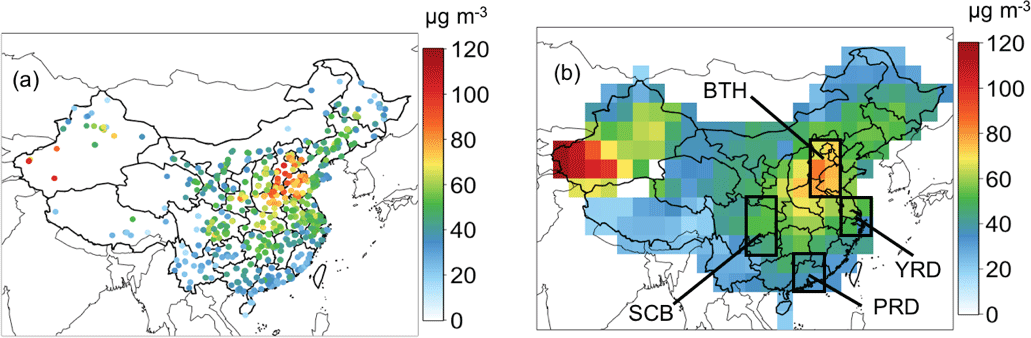
Figure 1Average (a) site and (b) gridded 2.5∘ × 2.5∘ total PM2.5 concentrations (µg m−3) of China during the years 2015–2016 obtained from the Chinese Ministry of Environmental Protection (MEP, http://pm25.in; last access: 2 July 2017). Gridded data are obtained by spatially interpolating site data using an inverse weighting method as in Tai et al. (2010). The four main regions of our study are indicated in panel (b): Beijing–Tianjin–Hebei (BTH), the Yangtze River Delta (YRD), the Pearl River Delta (PRD), and the Sichuan Basin (SCB).
In addition to local meteorological conditions, synoptic-scale circulation patterns also play important roles in driving PM2.5 variability. Different classification schemes for a wide range of synoptic circulation patterns have been researched extensively (Huth et al., 2008) and used worldwide to evaluate pollution–meteorology interactions (e.g., McGregor and Bamzelis, 1995; Shahgedanva et al., 1998; Shen et al., 2017; Tai et al., 2012a; Zhang et al., 2012). Tai et al. (2012a) showed that cold fronts associated with midlatitude cyclone passages and maritime inflows were the major ventilation mechanisms of PM2.5 in the US. Shen et al. (2017) further showed that the variability of PM2.5 over the USA explained by both local meteorology and synoptic factors (43 %) are on average about 10 % higher than solely using local meteorology (34 %). In Asia, Chen et al. (2008) demonstrated that synoptic high-pressure systems in northern Mongolia associated with cold fronts facilitate the dispersion of air pollutants over northern China, whereas a surface high centered on Beijing–Tianjin–Hebei (BTH) favors accumulation. Zhang et al. (2013) showed similar results by extracting nine distinct synoptic pressure patterns over the North China Plain (NCP), and discovered that weak pressure tendency in NCP favors pollutant accumulation. Zhang et al. (2016) found that a cold surge associated with the East Asian winter monsoon significantly reduced PM2.5 concentration in Beijing by 110 µg m−3 within a few days. Moreover, the effects of local meteorology and synoptic circulation are not independent of each other. For instance, Tai et al. (2012a) found that much of the apparent observed correlation of PM2.5 with temperature and pressure in the eastern USA are attributable to common association with cold frontal passages. To understand how meteorological changes may affect future PM2.5 air quality, therefore, requires keen consideration of the co-variation of meteorological variables with synoptic-scale phenomena in an integrated framework (Jiang et al., 2005).
Table 1Meteorological variables considered in this studya.
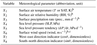
a From the National Center for Environmental Prediction/National Center for Atmospheric Research (NCEP/NCAR) Reanalysis 1 for 1998–2017. All data are 24 h averages and are deseasonalized as described in the text. b Surface data are from 0.995 sigma level. c Calculated from the horizontal wind vectors (u, v). d θ is the angle of the horizontal wind vector counterclockwise from the east. Positive values of X7 and X8 indicate westerly and southerly winds, respectively.
In this study, we perform correlation analysis to estimate the sensitivities of observed daily total PM2.5 to a suite of meteorological variables from June 2014 to May 2017. As discussed in Sect. 3, however, correlations between local meteorology and PM2.5 are complicated by co-variations among individual meteorological variables, which are at least partially driven by synoptic systems. We therefore apply principal component analysis to construct different meteorological modes that differentiate between unique synoptic-scale meteorological regimes, and we apply principal component regression (PCR) of daily PM2.5 on these modes to not only interpret the observed correlations of daily PM2.5 with individual meteorological variables, but also to determine the dominant meteorological modes of daily PM2.5 variability, in four major city clusters of China: BTH, the Yangtze River Delta (YRD), the Pearl River Delta (PRD), and the Sichuan Basin (SCB; Fig. 1). Furthermore, using BTH as a case study, we undertake spectral analysis of the time series of dominant meteorological modes over the past decade to examine the interannual correlations between synoptic frequencies and annual mean PM2.5. We finally construct a statistical model using annual median synoptic frequency and annual mean local meteorology to project 2000–2050 PM2.5 changes given present-day and future climate simulations by an ensemble of climate models. This study represents an advancement over that of Tai et al. (2012a, b) in terms of methodology by considering the joint effects of synoptic frequency and local meteorology, on par with Shen et al. (2017), which, however, focused only on the US. Our work represents the first attempt to apply these methods to Chinese air quality in an effort to derive a statistical projection of future PM2.5 concentrations based on historical PM2.5–meteorology relationships. These historical relationships can also be used to compare results from process-based models (e.g., Jiang et al., 2013).
Daily assimilated meteorological fields for 1998–2017 over China are obtained from National Centers for Environmental Prediction/National Center for Atmospheric Research (NCEP/NCAR) Reanalysis 1 provided by the National Oceanic and Atmospheric Administration (NOAA) of the USA (Kalney et al., 1996). The dataset has a horizontal resolution of 2.5∘ × 2.5∘. Following Tai et al. (2012a, b), eight meteorological variables are considered here (Table 1), including surface air temperature (X1), relative humidity (X2), precipitation rate (X3), sea-level pressure (X4), pressure tendency (X5), wind speed (X6), and two wind direction indicators (X7, X8). To conduct correlation analysis and PC regression, meteorological data, except from variables X5, X7 and X8, are deseasonalized and detrended by subtracting the corresponding centered 31-day moving averages from the original data to focus on day-to-day, synoptic-scale variability. Specifically, for a meteorological variable Xk in any grid, the deseasonalized meteorology is calculated as follows:
The deseasonalized and detrended data are also normalized to their standard deviations to yield zero means and unit variances:
where represents the normalized meteorological time series, and are the mean and standard deviation of the deseasonalized time series, respectively.
PM2.5 monitoring has been introduced in the national air quality monitoring network in China since 2012 with the published third revision of the National Ambient Air Quality Standards (NAAQS; Zhang and Cao, 2015). Before that, observational spatial distribution of PM2.5 was mostly estimated by satellite retrievals (Ma et al., 2015; van Donkelaar et al., 2010; Xue et al., 2017; Zheng et al., 2016). One of the disadvantages of PM2.5 monitoring at present is that there are very few sites with detailed speciation data in China, although short-term studies of PM2.5 speciation have been conducted (Cao et al., 2012b; Huang et al., 2014; Yang et al., 2005, 2011; J. K. Zhang et al., 2014). In this study, hourly mean data of total PM2.5 from 1 June 2014 to 30 May 2017 are obtained from the Chinese Ministry of Environmental Protection (MEP). Data are archived from 1497 monitors across China (Fig. 1a), most of which are concentrated in eastern, northeastern, and southern China, and are made available through a repository website (http://pm25.in; last access: 2 July 2017). We cross-check and correct the locations of the different monitoring sites, removing unrealistic values and instrumental errors. PM2.5 data are then deseasonalized and detrended in the same way as for the meteorological variables.
To conduct the statistical analysis, MEP observations are interpolated using inverse distance weighting onto the same 2.5∘ × 2.5∘ resolution as that for the NCEP/NCAR data to produce daily mean PM2.5 fields for 2014–2017. Sampled values (zj) from sites within a search distance (dmax) are weighted inversely by their distances (di) from the cell centroid to produce an average (zj) for each grid cell j:
where nj is the number of sampled sites for grid cell j and k is the power parameter. We choose k=2 and dmax=500 km as recommended by Tai et al. (2010). Figure 1 shows the averaged site and interpolated PM2.5 values for 2015 and 2016. As shown in Fig. 1, sites in much of southwestern China (e.g., in the provinces of Tibet and Qinghai) are relatively sparse, leading to likely unrepresentative interpolated values in the corresponding grid cells. These regions are excluded from our analysis.
For the purpose of examining long-term interannual PM2.5 variability, we also make use of the annual mean concentrations of surface total PM2.5 for 1998–2015 derived from satellite measurements (van Donkelaar et al., 2016). Total column aerosol optical depth (AOD) retrievals from multiple satellite instruments and model simulations, such as the MODerate resolution Imaging Spectroradiometer (MODIS), the Multiangle Imaging SpectroRadiometer (MISR), and the GEOS-Chem chemical transport model, were weighted by the ground-based AOD observations from the Aerosol Robotic Network (AERONET) sun photometers. The daily AOD and near-surface PM2.5 were simulated by GEOS-Chem to obtain the AOD-PM2.5 relationship, which were applied to the satellite AOD retrievals to yield weighted PM2.5 concentrations. Annual mean values of PM2.5 were computed and then calibrated to ground-based PM2.5 observations using the global geographically weighted regression (GWR) method (Brunsdon et al., 1996). Figure S1 in the Supplement shows the spatial variation of the satellite-derived PM2.5 over China from van Donkelaar et al. (2016), which has a spatial correlation of r=0.79 with MEP total PM2.5 for year 2015.
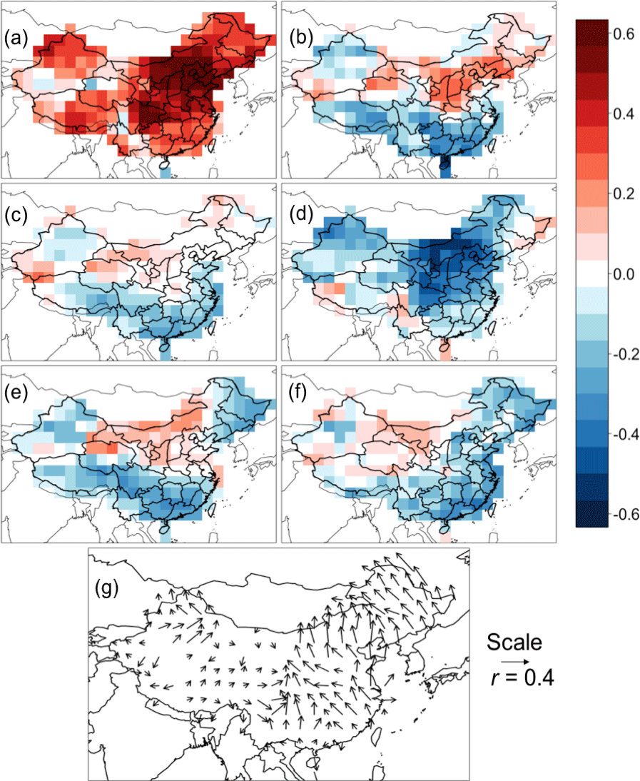
Figure 2Correlation coefficients of daily PM2.5 with different meteorological variables in Table 1, including (a) surface air temperature (X1, K), (b) relative humidity (X2, %), (c) precipitation (X3, mm d−1), (d) sea level pressure (X4, hPa), (e) pressure tendency (X5, hPa d−1), (f) wind speed (X6, m s−1), and (g) wind direction (X7 and X8, unitless), for China from June 2014 to May 2017. PM2.5 data are from MEP. Meteorological data are deseasonalized by subtracting 31-day moving averages and normalized, and daily total PM2.5 are also deseasonalized the same way to focus on day-to-day variability. Only values with significant correlations at p value ≤ 0.05 are shown. Panel (g) is plotted by finding the vector sums of the correlation coefficients for X7 and X8, with positive correlations pointing eastward and northward, respectively. The direction of the vector sum indicates the prevalent wind direction when PM2.5 has a positive anomaly.
To project the 2000–2050 effect of climate change on future PM2.5, we use the meteorological variables in Table 1 archived from an ensemble of 15 climate models participating in the Coupled Model Intercomparison Project Phase 5 (CMIP5) under the representative concentration pathway 8.5 (RCP8.5). We regrid the data from different models into the same 2.5∘ × 2.5∘ resolution. The details of the models can be found in Table S1 in the Supplement.
Here we first discuss the general correlation patterns between PM2.5 and individual meteorological variables in China, and highlight what we can and cannot conclude from them. The Pearson's correlation coefficients between each meteorological variable in Table 1 and interpolated daily total PM2.5 are computed for each grid cell from June 2014 to May 2017.
Figure 2 shows the correlation maps for the whole period. Temperature is found to have an overall significant positive correlation with deseasonalized PM2.5 in most regions of China (Fig. 2a), with the highest values appearing in BTH and SCB (r=0.6). The correlation map of SLP (Fig. 2d), which is often an indicator of the passages of synoptic systems, has a similar spatial pattern to that with temperature but with an opposite sign and smaller magnitudes, suggesting that PM2.5 tends to be low when SLP is high. The anticorrelation pattern is relatively weaker in southern China. Temperature and SLP are themselves found to be significantly negatively correlated throughout most of China (Fig. S2), and thus it is difficult to conclude whether they are the direct physical drivers of PM2.5 variability, or the correlations simply reflect common association with larger meteorological regimes that control PM2.5 variability.
Correlation between RH and PM2.5 shows different patterns in northern vs. southern China (Fig. 2b). A positive correlation (r=0.4) is seen in BTH, likely reflecting higher PM water content in ambient air which can enhance the uptake of semivolatile components (Dawson et al., 2007b), consistent with previous findings (Wang et al., 2014). In southern China, however, RH is negatively correlated with PM2.5, with larger correlations in SCB and PRD () than in YRD (). As can be seen in Fig. 2c, negative correlation of precipitation with PM2.5 in southern China is very similar to that of RH in Fig. 2b, likely reflecting the association of high RH with precipitation (Fig. 2c) and onshore wind (Fig. 2f), which can facilitate PM2.5 deposition or ventilation (Zhu et al., 2012). Such a strong association between RH and precipitation may also explain the apparently positive correlation between precipitation and PM2.5 in northern China, where RH-promoted aerosol formation is likely more important than wet deposition in the overall relationship.
Pressure tendency and wind speed exhibit similar correlation patterns (Fig. 2e–f). Pressure tendency, another indicator of synoptic-scale motions, is negatively correlated with PM2.5 in southern China, including PRD () and in northeastern China, suggesting that PM2.5 tends to be low when SLP is increasing. Wind speed is also negatively correlated with PM2.5 in similar regions. These patterns are consistent with advecting cold fronts with strong winds helping to ventilate PM2.5 in heavily polluted regions (Tai et al., 2012a). Pressure tendency and wind speed have a positive correlation with PM2.5 in northern China and some parts of western China, which may be due to the co-varying strong winds and frontal passages promoting the mobilization of mineral dust from the semiarid regions and deserts there.
Figure 2g shows the correlation of wind direction with PM2.5, in which arrow directions indicate wind directions associated with increasing PM2.5. The corresponding mass divergence map together with its calculation is shown in the Supplement (Fig. S3). For instance, PM2.5 increases with southeasterly wind for all of eastern and northeastern China with a correlation of r=0.3 on average. This relationship suggests that northwesterly wind tends to ventilate PM2.5 in most of China. Two divergent wind patterns are seen, one in central China and one in Taklamakan Desert, and their positions mirror regions with the highest PM2.5 concentrations in Fig. 1b. This result implies that wind transports pollutants from source regions to the peripheries.
A generally consistent correlation among neighboring grid cells may be associated with synoptic effects because the correlation pattern extends to a synoptic regional length scale. The correlation maps for most of the meteorological variables in Fig. 2 show such an effect. The commonality among the correlation patterns of PM2.5 with different meteorological variables, which among themselves have various degrees of correlation, renders the interpretation of individual PM2.5–meteorology relationships more difficult because the true driver of PM2.5 variability may be masked by the collinearity among meteorological variables (as is pointed out above for the case of temperature and SLP). Whenever a strong correlation between PM2.5 and a given meteorological variable (e.g., temperature, RH, precipitation, wind speed) is found, there can be three interpretations: (1) this variable is truly the physical driver for PM2.5 variability; (2) at least part of the correlation may arise from the correlation of this variable with another local variable that is the true physical driver; and (3) at least part of the correlation may reflect common association with a larger, synoptic-scale phenomenon that drives PM2.5 variability. To quantitatively differentiate between these possibilities and to ascertain the roles of local meteorology vs. synoptic-scale circulation on PM2.5 variability, we conduct principal component analysis (PCA) on the eight meteorological variables to capture their common co-variations in an ensemble of independent meteorological modes. We follow Tai et al. (2012a), and regress daily PM2.5 on the resulting principal component (PC) time series to identify the dominant synoptic drivers of PM2.5 variability. Their approach is particularly useful in that it enables the quantification of the fraction of PM2.5 variability that can be explained by synoptic meteorological regimes.
We perform PCA on the eight meteorological variables for 1998–2017 in Table 1 to extract synoptic circulation patterns, focusing on the four major metropolitan regions in China (BTH, YRD, PRD, and SCB). We use this longer period of meteorological data for the PCA despite the relatively short time history of PM2.5 data from MEP (2014–2017) because we aim to characterize the climatologically important synoptic systems in China. The longer period also overlaps with the annual mean PM2.5 data available for quantifying interannual variability (see Sect. 5), so that a unified set of meteorological modes can be used to explain both daily and interannual PM2.5 variability. We conduct PCA for individual seasons and for the whole period. All gridded daily meteorological data are spatially averaged over the grid cells covering each of the four regions, deseasonalized, and normalized to yield zero means and unit variances, as described above. The resulting time series for each region are then decomposed to produce the PC time series (Uj=U1, …, U8):
where represents the deseasonalized regionally averaged meteorological fields in Table 1, and are the temporal mean and standard deviation of , is the normalized value of , and αkj is the elements of the transformation matrix (i.e., eigenvector or empirical orthogonal function, EOF) of PCA. The PC time series are ranked by their variances λ, with the leading three to four PCs capturing most of the meteorological variability (Wilks, 2011). For example, the first four PCs for the BTH region explain 76 % of the total meteorological variability. The last few PCs with variances λ < 1 are truncated using Kaiser's rule since they likely represent noises (Wilks, 2011). Each PC represents a distinct meteorological mode, the physical meaning of which is reflected by the values of αkj in Eq. (2) and verified by cross-examination of synoptic weather maps.
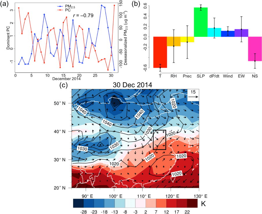
Figure 3Annually dominant meteorological mode for observed PM2.5 variability in Beijing–Tianjin–Hebei (BTH). (a) Time series of deseasonalized observed total PM2.5 concentrations and the principal component (PC) time series in the sample month of December 2014. (b) Composition of this mode as determined by the coefficients αkj, with error bars showing 2 standard deviations of the eigenvector coefficients. Meteorological variables are listed in Table 1. (c) Synoptic weather map on 30 December 2014 with temperature (K) as shaded colors, wind speed (m s−1) as vectors, and sea level pressure (hPa) as contours. The rectangle indicates BTH. The weather map, which shows an example of positive influence of the mode, is plotted using NCEP/NCAR reanalysis I data.
For each region, we then extract the PCs for 2014–2017 only, and construct a PCR model for deseasonalized, regionally averaged daily PM2.5 (, µg m−3) on the daily PC values (Uj) for 2014–2017, both for the whole period and for individual seasons:
where βj is the regression coefficient (µg m−3), and N the number of PCs retained after truncation (mostly 3 to 4).
We define a dominant meteorological mode seasonally or annually by computing the ratio of the resulting regression sum of squares (SSRj) to total sum of squares (SST) for each PC:
This ratio characterizes the fraction of variance of daily PM2.5 that can be explained by the jth PC in the PCR model. The PC with the largest SSR/SST is deemed the dominant meteorological mode for that region. Any PC which has an SSR/SST more than half of that of the dominant PC in a given season is also recognized as an important PC for that region. The total percentage of PM2.5 variability explained by the K dominant synoptic modes in a region can be written as
The PCR model also allows us to separate between synoptically driven and locally driven PM2.5 variability from the total meteorologically driven PM2.5 variability. Regressing PM2.5 using all eight individual meteorological variables yields a total R2 value, which entails both synoptically and locally driven PM2.5 variability, as discussed in Sect. 3. Using R2 and from the PCR model, we can infer the variability explained by local meteorology alone unrelated to synoptic modes, using
where indicates the overall locally driven PM2.5 variability.
Here we discuss the synoptic meteorological systems that dominate PM2.5 variability on annual timescales for each region. Discussion of regimes that control PM2.5 on seasonal timescales, as well as information on the values of SSR/SST and β, is included in the Supplement. We also note that in our interpretation, we focus only on the physical effects of meteorological phenomena. Non-physical drivers such as anthropogenic emissions can be correlated with meteorology to some extent (e.g., cold weather leading to higher emissions from heating); such effects, if any, would be encapsulated in the statistical model, but are difficult to diagnose explicitly due to a lack of corresponding data.
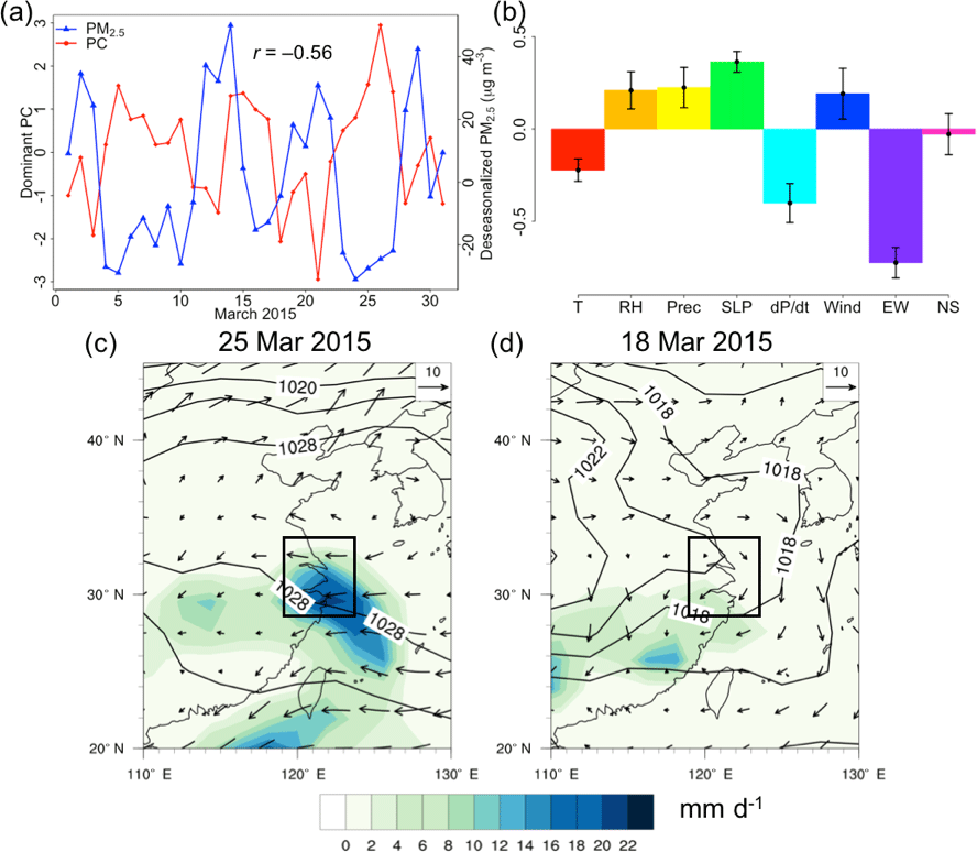
Figure 4Same as Fig. 3 but for the Yangtze River Delta (YRD). (a) Deseasonalized total PM2.5 concentrations and the PC time series in the sample month of March 2015. (b) Composition of this dominant mode as determined by the coefficients αkj. (c–d) Synoptic weather charts on 25 and 18 March 2015, with precipitation (mm d−1) shown as shaded colors, wind speed (m s−1) as vectors, and sea level pressure (hPa) as contours. Panel (c) shows the positive influence characterized by onshore wind with rainfall that corresponds to decreasing PM2.5, while panel (d) shows the negative influence with little wind on YRD. The rectangles indicate YRD.
Figure 3 shows the dominant meteorological mode in BTH, which explains nearly 36 % of PM2.5 variability throughout the year. Figure 3a shows a strong anticorrelation between the time series of this mode and deseasonalized observed total PM2.5 for the sample month of December 2014. Figure 3b shows the meteorological composition of the EOF of this annually dominant mode, with a positive phase consisting of low temperature, high SLP, and strong northwesterly winds. The error bars represent two standard errors of the meteorological composition, computed by the formula shown in Sect. S1 in the Supplement. Similar loadings are seen for winter, spring, and fall. We choose 30 December 2014 as a representative day with PC changing from negative to positive phase to explain the physical meaning of this PC. As seen in the weather map (Fig. 3c), the positive phase of the PC represents a high-pressure system associated with the Siberian High with dry cold fronts sweeping across BTH from northwest to southeast. The Siberian High is the driver of the winter monsoon in East Asia, and such northwesterly flow efficiently advects PM2.5 across BTH. Figure 3c shows a strongly decreasing temperature gradient and increasing pressure tendency originating from the Siberian High. PM2.5 concentration decreases by nearly 240 µg m−3 over 29 to 31 December (Fig. 3a). Regressing PM2.5 on all eight individual meteorological variables yields an R2 value of 43 %, indicating that local meteorology only contributes to an extra 7 % of the PM2.5 variability in addition to that already explained by synoptic circulation. In addition to cold fronts from the Siberian High, easterly onshore flow with high humidity and southerly monsoon also controls daily PM2.5 variability in spring and summer, explaining 18 and 17 % springtime and summertime variability of PM2.5, respectively (see Sect. S2).
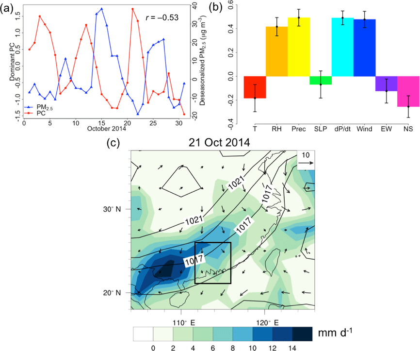
Figure 5Same as Fig. 3 but for fall in the Pearl River Delta (PRD). (a) Deseasonalized total PM2.5 concentrations and the PC time series in the sample month of October 2014. (b) Composition of this dominant mode as measured by the coefficients αkj. (c) Synoptic weather map on 21 October 2014, corresponding to the positive influence from the mode, with precipitation (mm d−1) as shaded colors, wind speed (m s−1) as vectors, and sea level pressure (hPa) as contours. The rectangle indicates PRD.
Figure 4 shows the dominant mode in YRD. This mode is important in spring, fall, and winter, and contributes up to 14 % of the PM2.5 variability for the whole year. The two time series of the PC and PM2.5 demonstrate anticorrelation with each other in March 2015 (Fig. 4a). The positive phase of this mode consists of low temperature, high RH and rainfall, high and decreasing pressure, and strong easterly winds (Fig. 4b). This set of meteorological phenomena is characteristic of onshore flow with rainfall, as demonstrated by the weather map on 25 March 2015, which shows cold and moist easterly winds originated from the high pressure centered over the East China Sea. Such winds sweep away pollutants and decrease PM2.5 concentration by 30 µg m−3 (Fig. 4c), and the associated rainfall also wash out PM2.5. The negative phase of this mode, as represented on 18 March 2015, shows anticyclonic flow leading to accumulation of PM2.5 (Fig. 4d). Local meteorology is found to contribute to an additional 11 % of the PM2.5 variability on top of that explained by synoptic effects. In addition to onshore flow, PCA for summer alone indicates that summertime low-pressure systems also deplete PM2.5, likely due to the associated precipitation, explaining 24 % of summertime PM2.5 variability. This PC is also sometimes characterized by northward-propagating tropical cyclones, with strong wind and rainfall (see Sect. S3).
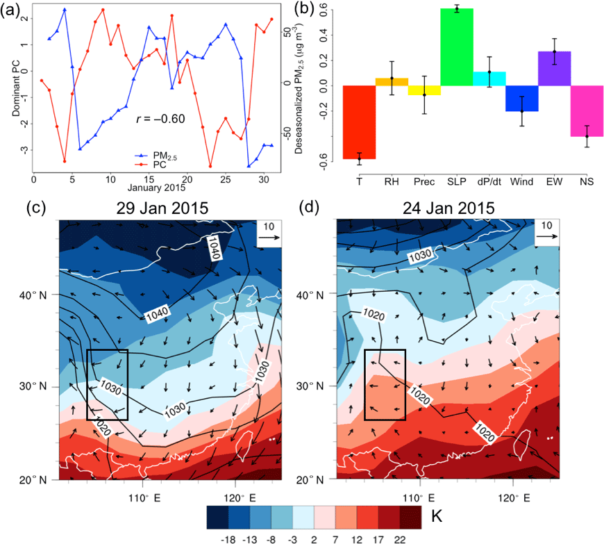
Figure 6Same as Fig. 3 but for winter in the Sichuan Basin (SCB). (a) Deseasonalized total PM2.5 concentrations and the PC time series in the sample month of January 2015. (b) Composition of this dominant mode as measured by the coefficients αkj. (c–d) Synoptic weather maps on 29 and 24 January 2015. Panel (c) shows the positive influence characterized by a cold front from the Siberian High that advects PM2.5 away, while panel (d) shows the negative influence characterized by stagnation over SCB. Temperature (K) is shown as shaded colors, wind speed (m s−1) as vectors, and sea level pressure (hPa) as contours. The rectangles indicate SCB.
Figure 5 shows the dominant mode for explaining PM2.5 variability in PRD. This mode is dominant in spring, fall, and winter, and in total contributes 22 % of variability in PM2.5 throughout the year. Figure 5a reveals a negative correlation between the PC for this mode and PM2.5 in October 2014. The positive phase of this mode consists of high RH, precipitation, increasing pressure, and strong northerly winds (Fig. 5b). This set of meteorological phenomena represents a cold frontal rainstorm, as demonstrated by the weather map in Fig. 5c, which shows a frontal rain belt coinciding with the positive phase of the PC on 21 October 2014. Pressure contours were advected southward by northerly winds, and a regional rain belt brought maximum rainfall of up to 15 mm d−1 to southern China. In general for this mode, advancing cold air sweeps from north to south and lifts the warmer and moister air, leading to precipitation and sometimes thunderstorms. Annually, regressing PM2.5 on individual meteorological variables yields an R2 value of 33 %; thus local meteorology contributes to an extra 11 % of PM2.5 variability unexplained by synoptic circulation. In addition to cold frontal rainstorms, summertime PCA also shows that the air quality in summer PRD is also influenced by rainfall from low-pressure troughs as well as by landfalls of tropical cyclones (see Figs. S11, S12). These two modes explain 18 and 15 % of summertime PM2.5 variability, respectively. The troughs cause rainfall that scavenges pollutants; tropical cyclones making landfall to the east of PRD cause inversion layers that trap pollutants and degrade air quality (see Sect. S4).
Figure 6 shows the dominant mode in SCB in winter, which has a negative correlation with PM2.5, as shown for the sample month of January 2015 (Fig. 6a). This mode dominates PM2.5 variability year-round, explaining 25 % of its day-to-day variability. PCA shows that its positive phase is characterized by low temperature, high SLP, and weak northwesterly winds (Fig. 6b), which resembles the dominant EOF in BTH. This mode is characterized by a northwesterly flow also associated with the Siberian High. On 29 January 2015, the Siberian High was situated southeast of Lake Baikal (Fig. 6c), advecting a clean, northwesterly cold front toward SCB and ventilating PM2.5 by 150 µg m−3 over 25 to 29 January. On 24 January, this mode was in its negative phase and SCB was under a relatively mild weather (Fig. 6d), while PM2.5 was at a local maximum (Fig. 6a). Annually, local meteorology contributes to another 20 % of the total PM2.5 variability. In addition to cold frontal passages, rainfall also drives PM2.5 variability especially in winter and spring, explaining 18 and 16 % of wintertime and springtime PM2.5 variability, respectively. This mode represents a cold frontal rain system that promotes wet deposition of pollutants (see Sect. S5).
Future climate change can significantly affect synoptic-scale circulation patterns and local meteorology, modifying the transport and deposition of PM2.5 (Fiore et al., 2015; Jiang et al., 2013; Mickley et al., 2004). Based on the demonstrated strong relationships of synoptic circulation and local meteorology on daily PM2.5, we build a regression model to infer how interannual variations of local and synoptic meteorology affect interannual PM2.5 variability, which we then apply to future climate projections. This approach allows us to evaluate the potential impacts of climate change on PM2.5 air quality. Here we adopt the PCA spectral analysis approach, namely, to apply a fast Fourier transform (FFT) to the daily time series of the dominant PCs for all seasons to extract the median frequencies from the resulting spectra. We use the same PCs generated using the 1998–2017 NCEP/NCAR meteorological data (Sect. 4), and smooth the resulting FFT spectra with a second-order autoregressive filter (Wilks, 2011). We focus on BTH as a case study. For example, spectral analysis shows that the Siberian High fluctuates between 58 and 67 times per year on average, and has a climatological frequency of 63 times per year averaged over 1998–2015.
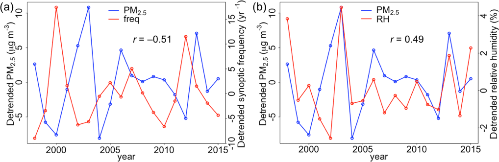
Figure 7Detrended annual mean total PM2.5 concentration and climate variables chosen by the forward selection model of 1998–2015, including (a) annual mean frequency of springtime Siberian High () and (b) relative humidity (r=0.49). Annual mean surface PM2.5 concentrations are derived from satellite AOD by van Donkelaar et al. (2016). All variables are detrended by subtracting the 7-year moving averages from the annual mean values.
Table 2Regression model that explains interannual variability of satellite-derived PM2.5 in Beijing–Tianjin–Hebei (BTH).
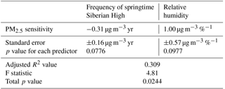
Satellite-retrieved PM2.5 has large uncertainties in seasonal mean values, and thus we make use of only the annual mean PM2.5 values for building our regression model. We construct a multiple linear regression (MLR) model for the 1998–2015 satellite-retrieved annual mean PM2.5 over BTH by spatially averaging the grid boxes covering the region. In selecting predictor variables, we consider the annual mean local meteorological variables in Table 1 (except SLP tendency, X5, and the two wind direction indicators, X7 and X8, whose averages are often nearly zero) and the annual median frequencies of synoptic circulation patterns from all individual seasons diagnosed from spectral analysis. The predictand (annual mean PM2.5) and potential predictors are detrended by subtracting from them the respective 7-year moving averages in order to remove long-term trends driven by emission changes. We adopt a forward selection approach (Wilks, 2011) to identify which climatic variables explain the greatest amount of interannual PM2.5 variability, starting from the one explaining the largest percentage of PM2.5 variability (having the largest adjusted R2 value), and adding predictor variables until the enhancement in adjusted R2 given by an additional predictor is less than 0.05. Variables that lead to a large variance inflation factor (> 2) are also excluded to avoid the issue of multicollinearity, which often leads to higher imprecision of regression estimates. Typically the forward selection algorithm does not yield more than three predictor variables for interannual PM2.5 variability.

Figure 8Projected changes in PM2.5 from 2000 to 2050, as calculated from meteorological outputs from the CMIP5 model ensemble. (a) Future projections of mean relative humidity (RH, %) and median synoptic frequency of springtime Siberian High (yr−1) as computed by 15 CMIP5 models. (b) Statistical distributions of CMIP5-projected RH and synoptic frequency as computed by model weighting algorithm of Tebaldi et al. (2005). (c) Changes in PM2.5 (µg m−3) from 2000 to 2050 based on climate projections from 15 models and statistical sensitivities from our multiple linear regression model. (d) Statistical distributions of projected PM2.5 based on Monte Carlo sampling of all possible uncertainty spaces. Dashed lines indicates the simple ensemble mean of the changes, red dots indicate positive changes, and blue dots indicate negative changes. The label “RH” indicates changes associated with relative humidity, “freq” indicates changes associated with frequency of cold fronts from the Siberian High, and “total” denotes the sum of the two.
Table 2 shows the interannual PM2.5 variability explained by the predictors, the corresponding regression coefficients and the p values for the BTH region. The two predictors selected by the forward selection algorithm are the frequency of the first PC in spring (i.e., the springtime Siberian High, Fig. S5) and annual mean RH. Figure 7 shows the correlation of detrended annual mean PM2.5 with detrended annual mean RH and the frequency of fluctuation of the springtime Siberian High. The negative correlation () between springtime PC frequency and annual PM2.5 indicates that more frequent occurrences of cold advection from the high-pressure systems further north, especially during spring, help ventilate PM2.5 in BTH and influence annual mean PM2.5 here. This is consistent with the relationship we found between PM2.5 and Siberian High on the daily timescale (Sect. 4). Annual mean RH has a positive correlation with PM2.5 (r=0.49), which is consistent with Sect. 3 where we found higher RH coinciding with higher PM2.5 on the daily timescale. Adding RH helps explain an additional 9 % of interannual PM2.5 variability, and the two predictors in total give an adjusted R2 value of 31 %, which represents a reasonably high value for a linear model, given that nonlinear PM2.5–meteorology interactions and emission-driven PM2.5 variability are not included in the model. Although temperature has a strong daily correlation of r=0.6 with PM2.5 in the correlation analysis in Sect. 3, annual mean temperature does not appear to correlate significantly with annual mean PM2.5 (r=0.18) and was not selected by the forward selection algorithm. Annual mean temperature also has a weak correlation with springtime Siberian High fluctuation frequency (), which indicates that more frequent synoptic fluctuations have only little bearing on annual mean temperature, and that the strong daily PM2.5–temperature co-variation is mostly a manifestation of synoptic influence. All other annual mean local meteorological variables have insignificant correlations with annual mean PM2.5.
Our findings show that meteorological effects on daily PM2.5 at least in part contribute to interannual variability PM2.5, a finding which we can utilize to estimate future changes in PM2.5. To this end, we extract the meteorological variables in Table 1 from the results of 15 models in the Climate Model Intercomparison Project Phase 5 (CMIP5) for 1996–2005 and 2046–2055 under the RCP8.5 scenario (Table S1). This scenario represents a business-as-usual future. We diagnose the 2000–2050 changes in the decadal averages of these variables and the median frequencies of the constructed PCs (Fig. 8a). To obtain an ensemble mean and distribution of the meteorological changes (Fig. 8b), we apply the weighting algorithm of Tebaldi et al. (2005) to the CMIP5 model outputs, which can discount any poorly performing models yielding meteorology that diverges from the present-day observations (using NCEP/NCAR reanalysis data in this study) or that diverges too much from the weighted ensemble mean, by giving those models a lower weight in the calculation of the ensemble mean and distribution.
We combine the meteorological changes with the PM2.5-to-climate sensitivities (i.e., regression coefficients in Table 2) to obtain an estimate for the 2000–2050 change in annual mean PM2.5 due to climate change alone (Fig. 8c), according to the following formula:
where ΔPM2.5 is the total PM2.5 change due to climate change, N is the total number of predictors selected by the forward selection algorithm, and Δxi is the change of the ith predictor selected by the algorithm. Here we make the “stationarity” assumption that the PM2.5-to-climate sensitivities, ∂PM, remain unchanged in the near future, such that ΔPM2.5 is totally due to changes in future meteorology. We then use a Monte Carlo approach to characterize the probability distribution and statistical significance of the changes in PM2.5 concentration arising from the uncertainties of the regression coefficients in the MLR model and from the differences in model physics among CMIP5 models. Our approach involves repeated (> 5000 times) sampling of regression coefficients of the MLR model from their distributions as parameterized by the means and standard errors in Table 2, along with the sampling of the performance-weighted ensemble distributions of meteorological changes from the Tebaldi et al. (2005) algorithm. The sampling distributions are aggregated in accordance with Eq. (9) to obtain the final distributions of PM2.5 changes for each predictor and the sum of the two (Fig. 8d).
Figure 8 shows the future changes of PM2.5 concentrations with the corresponding changes in future meteorology. Changes in RH among CMIP5 models show high inconsistency, with values ranging from −2.01 to +3.19 % (Fig. 8a). The ensemble mean of CMIP5 models shows a statistically insignificant increase (p value = 0.32) of RH of 0.23 ± 1.24 percentage points by 2050s in BTH (Fig. 8b), consistent with a future prediction of a change within < 1 % over BTH in the Fifth Assessment Report of Intergovernmental Panel on Climate Change (IPCC AR5; Fig. 12.21 in Collins et al., 2013). Past modeling studies show that RH remains nearly constant on climatological timescales and continental spatial scales (Randall et al., 2007), while recent investigation shows that near-surface RH decreases over most land areas globally (O'Gorman and Muller, 2010). IPCC AR5 (2013) shows that the regional mean RH in BTH changes by less than 1 standard deviation of interannual variability by year 2065, and the variability is dominated more by naturally occurring processes than by human activities.
We find that 10 of the 15 models project an increase in this synoptic frequency (Fig. 8a). Based on the weighting algorithm for discounting poorly performing models, we project an overall very likely (i.e., 90–100 % likelihood according to IPCC guideline in Stocker et al., 2013) statistically significant increase (p value = 0.0008) in the frequency of synoptic-scale fluctuation of the Siberian High by 1.46 ± 0.39 yr−1 by the 2050s (Fig. 8b). The generally increasing frequency is possibly driven by the future reduction in meridional temperature gradient, which decreases the intensity of the midlatitude jets and favors the amplification and persistence of surface anticyclones (e.g., Francis and Vavrus, 2012; Zhang et al., 2012). Francis and Vavrus (2012) showed that the upper tropospheric midlatitude jet (in the form of Rossby wave) exhibited reduced zonal velocity and augmented wave amplitude under warming over 1979–2010, which may have led to an increase in atmospheric blocking events (Barriopedro et al., 2006) and an enhancement in the likelihood of cold surges from the Siberian High. In another multi-model study, Park et al. (2011), however, found no significant correlation between cold surge occurrences and surface air temperature over East Asia, and thereby concluded that cold surge occurrences would remain constant in frequency under a warming climate. Our results based on PCA spectral analysis show a modest increase instead of unchanging frequency in synoptic-scale fluctuation of the Siberian High in the future.
Figure 8c and d show the corresponding future PM2.5 changes from the baseline value of 57.2 µg m−3 in the 2000s. Across the model results, we find an overall PM2.5 change of 0.21 to +1.79 µg m−3 due to changing RH, and of −0.29 to 0.63 µg m−3 due to changing synoptic frequency (Fig. 8c). From the Monte Carlo sampling of the performance-weighted distribution of meteorological changes and uncertainties of statistical parameters, the RH-induced PM2.5 change is 0.21 ± 1.44 µg m−3 (p value = 0.58), and the frequency-induced PM2.5 change is −0.46 ± 0.28 µg m−3 (p value = 0.028, 97 % likelihood; Fig. 8d). While the RH-induced PM2.5 change is statistically insignificant and its sign inconclusive, we show that the higher frequency of fluctuation in the Siberian High alone, through enhancing cold frontal frequency, could lead to a very likely reduction in annual mean PM2.5 and thus constitute a slight climate “benefit” for PM2.5 air quality over BTH of China. We find that the greatest uncertainty stems from large inter-model differences in the future projections of RH and, which are much larger than those in the synoptic frequency projections. The regression coefficients have relatively moderate standard errors (Table 2) and contribute only little to the overall projection uncertainty.
In this study we use a combination of multivariate statistical methods to investigate the local and synoptic meteorological effects on daily and interannual variability of PM2.5 in China. Based on the resulting statistical relationships between PM2.5 with annual mean meteorological variables and synoptic frequencies, we also project future PM2.5 changes in the Beijing–Tianjin–Hebei (BTH) region. First, we find strong correlations between daily observed PM2.5 and individual meteorological variables in China over 2014–2017, and the spatial patterns of correlations suggest common association of these variables with synoptic circulation and transport. We therefore apply PCA on spatially averaged meteorological variables for four major metropolitan regions (BTH, YRD, PRD, SCB) for 1998–2017 (for all seasons and for the whole period) to diagnose the dominant synoptic meteorological modes, and the time series of these modes are used as predictor variables in an MLR model to explain day-to-day PM2.5 variability for each region. We find that, in BTH, the presence of the Siberian High strongly controls PM2.5 levels. Northerly monsoonal flows and advecting cold fronts from the Siberian High play key roles in ventilating PM2.5 in BTH for all seasons except JJA. In YRD, onshore wind with precipitation from the East China Sea is the dominant meteorological mode, effectively scavenging PM2.5 for all seasons except JJA. In PRD, frontal rain is a key driver reducing PM2.5 by wet deposition for all seasons except JJA. In SCB, the Siberian High plays a key role in bringing clean air from the north that effectively dilutes pollution for all seasons. Different synoptic meteorological regimes in different seasons explain about 16–37 % of PM2.5 variability in 2014–2017.
We further show that the long-term fluctuations in the frequencies of the dominant synoptic modes also shape interannual variability of PM2.5. Using the BTH region as a case study, we use regionally averaged annual mean local meteorological variables and annual median frequencies of the dominant synoptic modes of all individual seasons as potential predictors in a forward-selection MLR model to explain the interannual variability of satellite-derived annual mean PM2.5 over 1998–2015. The forward selection model finds two significant predictors, namely, the frequency of springtime frontal passages (which indicates the interannual fluctuation in the strength of the Siberian High) and annual mean RH, with observed PM2.5-to-climate sensitivities of −0.31 ± 0.16 µg m−3 yr and 1.00 ± 0.57 µg m−3 %−1, which together explain 31 % of the variability of annual mean PM2.5. The signs of correlations between PM2.5 and the two predictors are also consistent with that from the daily PC regression analysis, showing a broad consistency in PM2.5–meteorology relationships across different timescales.
We further address the effect of 1996–2055 climate change on future PM2.5 air quality, using an ensemble of 15 CMIP5 climate model outputs under the RCP8.5 scenario. Ten out of 15 models show an increase in the frequency of strength fluctuation of the Siberian High with an ensemble mean of 1.46 yr−1. Nine out of 15 models show a statistically insignificant change in future RH. Inter-model differences in the projected changes in RH are much larger than that in synoptic frequency of fluctuation in the Siberian High, owing to the high inconsistency in future projections of atmospheric humidity, especially on a regional scale (IPCC, 2013). We combine the ensemble projection of RH and synoptic frequency with the PM2.5-to-climate sensitivity from our statistical model to project future PM2.5 changes, with uncertainties quantified using a Monte Carlo approach. While the RH-induced PM2.5 change is insignificant and inconclusive, we project for the 2050s a statistically significant and very likely (∼ 97 % likelihood) decrease in PM2.5 of −0.46 ± 0.28 µg m−3 due to increasing frequency in the fluctuation of the Siberian High. The overall projection is inconclusive mostly due to the highly uncertain RH projections. Our prediction is comparable in magnitude with other studies (e.g., Jiang et al., 2013) and predictions for the USA (Shen et al., 2017; Tai et al., 2012b; Pye et al., 2009; Avise et al., 2009) and Europe (Juda-Rezler et al., 2012), but much smaller in magnitude compared with the baseline value of 57.2 µg m−3 in the 2000s, suggesting that the “climate benefit” from higher synoptic frequency is rather small especially in comparison with what emission control efforts could do to curb PM2.5 concentrations in China. Jiang et al. (2013) projected changes of PM2.5 over China due to climate change alone under IPCC A1B scenario, and the resulting change over BTH is about +1 µg m−3 averaged annually. They attributed their predictions to (1) changing precipitation that leads to a change in wet deposition and (2) increasing temperature that results in more volatilization of nitrate and ammonium, which differs from our conclusion that cold frontal ventilation dominates the PM2.5–temperature correlation and total PM2.5 response. Our statistical results (for BTH only) do not show significant relationships between temperature and PM2.5 (r=0.18) nor between rainfall and PM2.5 (r=0.20) on an interannual timescale, despite strong correlations on a daily timescale. This discrepancy between empirical results and process-based model results may stem from the inadequacy of satellite-derived PM2.5 in capturing the variability caused by volatilization effect, an inadequate process-based model representation of the PM2.5–temperature relationship (Shen et al., 2017), and from the uncertainty in emissions of PM precursors in the process-based model.
There are two major limitations of the statistical approach developed in this study. First, due to accuracy constraints of the satellite-derived PM2.5 concentrations, we could only use annual mean PM2.5 instead of seasonal mean PM2.5 as the basis for interannual regression and future projections. Shen et al. (2017) showed that PM2.5 responds to meteorological conditions differently in different seasons in the US. Due to the short period of surface monitoring data (see Sect. 2), we rely on the annual mean satellite-derived PM2.5 with no seasonality in this study, and thus no seasonal predictions of PM2.5 are possible. Another limitation is that the statistical projections rely on the stationarity assumption that the PM2.5-to-climate sensitivities will be more or less constant in the future (see Eq. 7). This assumption may be acceptable for near-future projections (Fiore et al., 2012; IPCC, 2013), but it is less reliable for multidecadal projections especially as significant changes in emission levels may alter the chemical nature of total PM2.5 and thus the interactions with meteorology. While process-based modeling studies of the future evolution of PM2.5–meteorology relationships under varying levels of emissions in China are highly warranted, the empirical relationships as diagnosed from investigation of historical data in this study are valuable in providing a basis for testing and validating the process-based model sensitivities of PM2.5 air quality to climate change.
Data used in this study, including site-interpolated daily mean PM2.5, NCEP/NCAR Reanlaysis I meteorological data, and satellite-derived annual mean PM2.5, are deposited in the publicly available institutional repository, accessible via this link: http://www.cuhk.edu.hk/sci/essc/tgabi/data.html (Leung, 2018). Request for raw data or the complete set of data, or any questions regarding the data, can be directed to the principal investigator, Amos P. K. Tai (amostai@cuhk.edu.hk).
The supplement related to this article is available online at: https://doi.org/10.5194/acp-18-6733-2018-supplement.
The authors declare that they have no conflict of interest.
This work was supported by a faculty start-up allowance from the Croucher
Foundation and The Chinese University of Hong Kong (CUHK; project
ID: 6903601, 4930041) given to the principal investigator, Amos P. K. Tai, as
well as a Vice-Chancellor Discretionary Fund (project ID: 4930744) from CUHK
given to the Institute of Environment, Energy and Sustainability.
Edited by: Qiang Zhang
Reviewed by: two anonymous referees
Avise, J., Chen, J., Lamb, B., Wiedinmyer, C., Guenther, A., Salathé, E., and Mass, C.: Attribution of projected changes in summertime US ozone and PM2.5 concentrations to global changes, Atmos. Chem. Phys., 9, 1111–1124, https://doi.org/10.5194/acp-9-1111-2009, 2009.
Barriopedro, D., García-Herrera, R., Lupo, A. R., and Hernández, E.: A climatology of Northern Hemisphere blocking, J. Clim., 19, 1042–1063, 2006.
Brunsdon, C., Fotheringham, A. S., and Charlton, M. E.: Geographically Weighted Regression: A method for exploring spatial nonstationarity, Geogr. Anal., 28, 281–298, 1996.
Cao, J., Xu, H., Xu, Q., Chen, B., and Kan, H.: Fine particulate matter constituents and cardiopulmonary mortality in a heavily polluted Chinese city, Environ. Health Persp., 120, 373–378, 2012a.
Cao, J. J., Shen, Z. X., Chow, J. C., Watson, J. G., Lee, S. C., Tie, X. X., Ho, K. F., Wang, G. H., and Han, Y. M.: Winter and summer PM2.5 chemical compositions in fourteen Chinese cities, J. Air Waste Manage., 62, 1214–1226, 2012b.
Chan, C. K. and Yao, X.: Air pollution in mega cities in China, Atmos. Environ., 42, 1–42, 2008.
Chen, Z. H., Cheng, S. Y., Li, J. B., Guo, X. R., Wang, W. H., and Chen, D. S.: Relationship between atmospheric pollution processes and synoptic pressure patterns in northern China, Atmos. Environ. 42, 6078–6087, 2008.
Cohen, A. J., Brauer, M., Burnett, R., Anderson, H. R., Frostad, J., Estep, K., Balakrishnan, K., Brunekreef, B., Dandona, L., and Dandona, R.: Estimates and 25-year trends of the global burden of disease attributable to ambient air pollution: an analysis of data from the Global Burden of Diseases Study 2015, Lancet, 389, 1907–1918, 2017.
Collins, M., Knutti, R., Arblaster, J., Dufresne, J. L., Fichefet, T., Friedlingstein, P., Gao, X., Gutowski, W. J., Johns, T., Krinner, G., Shongwe, M., Tebaldi, C., Weaver, A., and Wehner, M.: Long-term climate change: Projections, commitments and irreversibility, in: Climate Change 2013: The Physical Basis, edited by: Stocker, T. F., Qin, D., Plattner, G.-K., Tignor, M., Allen, S. K., Boschung, J., Nauels, A., Xia, Y., Bex, V., and Midgley, P. M., Cambridge University Press, Cambridge, UK, 2013.
Leung, D. M.: Earth system Science Programme and Graduate Division of Earth and Atmospheric Sciences, The Chinese University of Hong Kong, http://www.cuhk.edu.hk/sci/essc/tgabi/data.htmlTS2 last access: 6 May 2018.
Dawson, J. P., Adams, P. J., and Pandis, S. N.: Sensitivity of PM2.5 to climate in the Eastern US: a modeling case study, Atmos. Chem. Phys., 7, 4295–4309, https://doi.org/10.5194/acp-7-4295-2007, 2007b.
Ding, X., Wang, X. M., Gao, B., Fu, X. X., He, Q. F., Zhao, X. Yu, J., and Zheng, M.: Tracer-based estimation of secondary organic carbon in the Pearl River Delta, south China, J. Geophys. Res., 117, D05313, https://doi.org/10.1029/2011JD016596, 2012.
Fiore, A. M., Naik, V., Spracklen, D. V., Steiner, A., Unger, N., Prather, M., Bergmann, D., Cameron-Smith, P. J., Cionni, I., Collins, W. J., and Dalsøren, S.: Global air quality and climate, Chem. Soc. Rev., 41, 6663–6683, 2012.
Fiore, A. M., Naik, V., and Leibensperger, E. M.: 2015 Annual A&WMA Critical Review: Air Quality and Climate Connections, J. Air Waste Manage., 65, 645–685, 2015.
Francis, J. A. and Vavrus, S. J.: Evidence linking Arctic amplification to extreme weather in mid-latitudes, Geophys. Res. Lett., 39, L06801, https://doi.org/10.1029/2012GL051000, 2012.
Fu, Y., Tai, A. P. K., and Liao, H.: Impacts of historical climate and land cover changes on fine particulate matter (PM2.5) air quality in East Asia between 1980 and 2010, Atmos. Chem. Phys., 16, 10369–10383, https://doi.org/10.5194/acp-16-10369-2016, 2016.
Han, L., Zhou, W., and Li, W.: Fine particulate (PM2.5) dynamics during rapid urbanization in Beijing, 1973–2013, Sci. Rep., 6, 23604, 2016.
Huang, R. J., Zhang, Y., Bozzetti, C., Ho, K. F., Cao, J. J., Han, Y., Daellenbach, K. R., Slowik, J. G., Platt, S. M., Canonaco, F., and Zotter, P.: High secondary aerosol contribution to particulate pollution during haze events in China, Nature, 514, 218–222, 2014.
Huth, R., Beck, C., Philipp, A., Demuzere, M., Ustrnul, Z., Cahynová, M., Kyselý, J., and Tveito, O. E.: Classifications of atmospheric circulation patterns, Ann. NY. Acad. Sci., 1146, 105–152, 2008.
IPCC: Fifth Assessment Report: Climate Change 2013: The Physical Science Basis, Contribution of Working Group I to the Fifth Assessment Report of the Intergovernmental Panel on Climate Change, edited by: Stocker, T. F., Qin, D., Plattner, G.-K., Tignor, M., Allen, S. K., Doschung, J., Nauels, A., Xia, Y., Bex, V., and Midgley, P. M., Cambridge University Press, 2013.
Jacob, D. J. and Winner, D. A.: Effect of climate change on air quality, Atmos. Environ., 43, 51–63, 2009.
Jiang, H., Liao, H., Pye, H. O. T., Wu, S., Mickley, L. J., Seinfeld, J. H., and Zhang, X. Y.: Projected effect of 2000–2050 changes in climate and emissions on aerosol levels in China and associated transboundary transport, Atmos. Chem. Phys., 13, 7937–7960, https://doi.org/10.5194/acp-13-7937-2013, 2013.
Jiang, N., Hay, J. E., and Fisher, G. W.: Synoptic weather types and morning rush hour nitrogen oxides concentrations during Auckland winters, Weather Clim. Soc., 25, 43–69, 2005.
Juda-Rezler, K., Reizer, M., Huszar, P., Krüger, B. C., Zanis, P., Syrakov, D., Katragkou, E., Trapp, W., Melas, D., Chervenkov, H., and Tegoulias, I.: Modelling the effects of climate change on air quality over Central and Eastern Europe: concept, evaluation and projections, Clim. Res., 53, 179–203, 2012.
Kalnay, E., Kanamitsu, M., Kistler, R., Collins, W., Deaven, D., Gandin, L., Iredell, M., Saha, S., White, G., Woollen, J., Zhu, Y., Chelliah, M., Ebisuzaki, W., Higgins, W., Janowiak, J., Mo, K. C., Ropelewski, C., Wang, J., Leetmaa, A., Reynolds, R., Jenne, R., and Joseph, D.: The NCEP/NCAR 40-year reanalysis project, B. Am. Meteorol. Soc., 77, 437–471, 1996.
Koch, D., Park, J., and Del Genio, A.: Clouds and sulfate are anticorrelated: A new diagnostic for global sulfur models, J. Geophys. Res., 108, p. 4781, 2003.
Krewski, D., Jerrett, M., Burnett, R. T., Ma, R., Hughes, E., Shi, Y., Turner, M. C., Pope III, C. A., Thurston, G., Calle, E. E., and Thun, M. J.: Extended follow-up and spatial analysis of the American Cancer Society study linking particulate air pollution and mortality, Res. Rep. Health. Eff. Inst., 140, 5–114, 2009.
Ma, Z., Hu, X., Sayer, A.M., Levy, R., Zhang, Q., Xue, Y., Tong, S., Bi, J., Huang, L., and Liu, Y.: Satellite-based spatiotemporal trends in PM2.5 concentrations: China, 2004–2013, Environ. Health Persp., 124, 184–192, 2015.
Madaniyazi, L., Nagashima, T., Guo, Y., Yu, W., and Tong, S.: Projecting fine particulate matter-related mortality in East China, Environ. Sci. Technol., 49, 11141–11150, 2015.
McGregor, G. R. and Bamzelis, D.: Synoptic typing and its application to the investigation of weather air pollution relationships, Birmingham, UK, Theor. Appl. Climatol., 51, 223–236, 1995.
Mickley, L. J., Jacob, D. J., Field, B. D., and Rind, D.: Effects of future climate change on regional air pollution episodes in the United States, Geophys. Res. Lett., 31, L24103, https://doi.org/10.1029/2004GL021216, 2004.
O'Gorman, P. A. and Muller, C. J.: How closely do changes in surface and column water vapor follow Clausius–Clapeyron scaling in climate change simulations?, Environ. Res. Lett., 5, 025207, https://doi.org/10.1088/1748-9326/5/2/025207, 2010.
Park, T. W., Ho, C. H., Jeong, S. J., Choi, Y. S., Park, S. K., and Song, C. K.: Different characteristics of cold day and cold surge frequency over East Asia in a global warming situation, J. Geophys. Res., 116, D12118, https://doi.org/10.1029/2010JD015369, 2011.
Pope III, C. A. and Dockery, D. W.: Health effects of fine particulate air pollution: lines that connect, J. Air Waste Manage., 56, 709–742, 2006.
Pye, H. O. T., Liao, H., Wu, S., Mickley, L. J., Jacob, D. J., Henze, D. K., and Seinfeld, J. H.: Effect of changes in climate and emissions on future sulfate-nitrate-ammonium aerosol levels in the United States, J. Geophys. Res., 114, D01205, https://doi.org/10.1029/2008JD010701, 2009.
Randall, D. A., Wood, R. A., Bony, S., Colman, R., Fichefet, T., Fyfe, J., Kattsov, V., Pitman, A., Shukla, J., Srinivasan, J., Stouffer, R. J., Sumi, A., and Taylor, K. E.: Climate Models and Their Evaluation, in: Climate Change 2007: The Physical Science Basis, Contribution of Working Group I to the Fourth Assessment Report of the Intergovernmental Panel on Climate Change, edited by: Solomon, S., Qin, D., Manning, M., Chen, Z., Marquis, M., Averyt, K. B., Tignor, M., and Miller, H. L., Cambridge University Press, Cambridge, United Kingdom and New York, NY, USA, 2007.
Seinfeld, J. H. and Pandis, S. N.: Atmospheric chemistry and physics: from air pollution to climate change, John Wiley & Sons, 2016.
Shahgedanova, M., Burt, T. P., and Davies, T. D.: Synoptic climatology of air pollution in Moscow, Theor. Appl. Climatol., 61, 85–102, 1998.
Shen, L., Mickley, L. J., and Murray, L. T.: Influence of 2000–2050 climate change on particulate matter in the United States: results from a new statistical model, Atmos. Chem. Phys., 17, 4355–4367, https://doi.org/10.5194/acp-17-4355-2017, 2017.
Stocker, T. F., Qin, D., Plattner, G.-K., Alexander, L. V., Allen, S. K., Bindoff, N. L., Bréon, F.-M., Church, J. A., Cubasch, U., Emori, S., Forster, P., Friedlingstein, P., Gillett, N., Gregory, J. M., Hartmann, D. L., Jansen, E., Kirtman, B., Knutti, R., Krishna Kumar, K., Lemke, P., Marotzke, J., Masson-Delmotte, V., Meehl, G. A., Mokhov, I. I., Piao, S., Ramaswamy, V., Randall, D., Rhein, M., Rojas, M., Sabine, C., Shindell, D., Talley, L. D., Vaughan, D. G., and Xie, S.-P.: Technical Summary, in: Climate Change 2013: The Physical Science Basis, Contribution of Working Group I to the Fifth Assessment Report of the Intergovernmental Panel on Climate Change edited by: Stocker, T. F., Qin, D., Plattner, G.-K., Tignor, M., Allen, S. K., Boschung, J., Nauels, A., Xia, Y., Bex, V., and Midgley, P. M., Cambridge University Press, Cambridge, UK and New York, NY, USA, 2013.
Tai, A. P. K., Mickley, L. J., and Jacob, D. J.: Correlations between fine particulate matte (PM2.5) and meteorological variables in the united states: Implications for the sensitivity of PM2.5 to climate change, Atmos. Environ., 44, 3976–3984, 2010.
Tai, A. P. K., Mickley, L. J., Jacob, D. J., Leibensperger, E. M., Zhang, L., Fisher, J. A., and Pye, H. O. T.: Meteorological modes of variability for fine particulate matter (PM2.5) air quality in the United States: implications for PM2.5 sensitivity to climate change, Atmos. Chem. Phys., 12, 3131–3145, https://doi.org/10.5194/acp-12-3131-2012, 2012a.
Tai, A. P. K., Mickley, L. J., and Jacob, D. J.: Impact of 2000–2050 climate change on fine particulate matter (PM2.5) air quality inferred from a multi-model analysis of meteorological modes, Atmos. Chem. Phys., 12, 11329–11337, https://doi.org/10.5194/acp-12-11329-2012, 2012b.
van Donkelaar, A., Martin, R. V., Brauer, M., Kahn, R., Levy, R., Verduzco, C., and Villeneuve, P. J.: Global estimates of ambient fine particulate matter concentrations from satellite-based aerosol optical depth: development and application, Environ. Health Persp., 118, 847–855, 2010.
van Donkelaar, A., Martin, R. V., Brauer, M., Hsu, N. C., Kahn, R. A., Levy, R. C., Lyapustin, A., Sayer, A. M., and Winker, D. M.: Global estimates of fine particulate matter using a combined geophysical-statistical method with information from satellites, models, and monitors, Environ. Sci. Technol., 50, 3762–3772, 2016.
Wang, L., Xu, J., Yang, J., Zhao, X., Wei, W., Cheng, D., Pan, X., and Su, J.: Understanding haze pollution over the southern Hebei area of China using the CMAQ model, Atmos. Env., 56, 69–79, 2012.
Wang, L., Zhang, N., Liu, Z., Sun, Y., Ji, D., and Wang, Y.: The influence of climate factors, meteorological conditions, and boundary-layer structure on severe haze pollution in the Beijing-Tianjin-Hebei region during January 2013, Adv. Meteorol., 2017, 1–14, 2014.
Wilks, D. S.: Statistical methods in the atmospheric sciences, Vol. 100, Academic Press, 2011.
Xu, P., Chen, Y., and Ye, X.: Haze, air pollution, and health in China, Lancet, 382, 2067, https://doi.org/10.1016/S0140-6736(13)62693-8, 2013.
Xue, T., Zheng, Y., Geng, G., Zheng, B., Jiang, X., Zhang, Q., and He, K.: Fusing Observational, Satellite Remote Sensing and Air Quality Model Simulated Data to Estimate Spatiotemporal Variations of PM2.5 Exposure in China, Remote Sens., 9, 221pp., 2017.
Yang, F., He, K., Ye, B., Chen, X., Cha, L., Cadle, S. H., Chan, T., and Mulawa, P. A.: One-year record of organic and elemental carbon in fine particles in downtown Beijing and Shanghai, Atmos. Chem. Phys., 5, 1449–1457, https://doi.org/10.5194/acp-5-1449-2005, 2005.
Yang, F., Tan, J., Zhao, Q., Du, Z., He, K., Ma, Y., Duan, F., Chen, G., and Zhao, Q.: Characteristics of PM2.5 speciation in representative megacities and across China, Atmos. Chem. Phys., 11, 5207–5219, https://doi.org/10.5194/acp-11-5207-2011, 2011.
Zhang, Q., Streets, D. G., He, K., and Klimont, Z.: Major components of China's anthropogenic primary particulate emissions, Environ. Res. Lett., 2, 045027, https://doi.org/10.1088/1748-9326/2/4/045027, 2007.
Zhang, R., Li, Q., and Zhang, R.: Meteorological conditions for the persistent severe fog and haze event over eastern China in January 2013, Sci. China Earth Sci., 57, 26–35, 2014.
Zhang, J. K., Sun, Y., Liu, Z. R., Ji, D. S., Hu, B., Liu, Q., and Wang, Y. S.: Characterization of submicron aerosols during a month of serious pollution in Beijing, 2013, Atmos. Chem. Phys., 14, 2887–2903, https://doi.org/10.5194/acp-14-2887-2014, 2014.
Zhang, J. P., Zhu, T., Zhang, Q. H., Li, C. C., Shu, H. L., Ying, Y., Dai, Z. P., Wang, X., Liu, X. Y., Liang, A. M., Shen, H. X., and Yi, B. Q.: The impact of circulation patterns on regional transport pathways and air quality over Beijing and its surroundings, Atmos. Chem. Phys., 12, 5031–5053, https://doi.org/10.5194/acp-12-5031-2012, 2012.
Zhang, J. P., Zhu, T., Zhang, Q. H., Li, C. C., Shu, H. L., Ying, Y., Dai, Z. P., Wang, X., Liu, X. Y., Liang, A. M., and Shen, H. X.: Sources and processes affecting fine particulate matter pollution over North China: an adjoint analysis of the Beijing APEC period, Environ. Sci. Technol., 50, 8731–8740, 2016.
Zhang, Y. L. and Cao, F.: Fine particulate matter (PM2.5) in China at a city level, Sci. Rep., 5, 1–11, 2015.
Zhang, X., Lu, C., and Guan, Z.: Weakened cyclones, intensified anticyclones and recent extreme cold winter weather events in Eurasia, Environ. Res. Lett., 7, 044044, https://doi.org/10.1088/1748-9326/7/4/044044, 2012.
Zheng, Y., Zhang, Q., Liu, Y., Geng, G., and He, K.: Estimating ground-level PM2.5 concentrations over three megalopolises in China using satellite-derived aerosol optical depth measurements, Atmos. Environ., 124, 232–242, 2016.
Zhu, J., Liao, H., and Li, J.: Increases in aerosol concentrations over eastern China due to the decadal-scale weakening of the East Asian summer monsoon, Geophys. Res. Lett., 39, L09809, https://doi.org/10.1029/2012GL051428, 2012.
- Abstract
- Introduction
- Data and methods
- Correlations between daily PM2.5 and meteorological variables
- Dominant meteorological modes for daily PM2.5 variability based on principal component regression
- Synoptic frequency and local meteorology as metrics for climate change impact on PM2.5
- Conclusions and discussion
- Data availability
- Competing interests
- Acknowledgements
- References
- Supplement