the Creative Commons Attribution 3.0 License.
the Creative Commons Attribution 3.0 License.
Meteorological controls on atmospheric particulate pollution during hazard reduction burns
Giovanni Di Virgilio
Melissa Anne Hart
Ningbo Jiang
Internationally, severe wildfires are an escalating problem likely to worsen given projected changes to climate. Hazard reduction burns (HRBs) are used to suppress wildfire occurrences, but they generate considerable emissions of atmospheric fine particulate matter, which depend upon prevailing atmospheric conditions, and can degrade air quality. Our objectives are to improve understanding of the relationships between meteorological conditions and air quality during HRBs in Sydney, Australia. We identify the primary meteorological covariates linked to high PM2.5 pollution (particulates < 2.5 µm in diameter) and quantify differences in their behaviours between HRB days when PM2.5 remained low versus HRB days when PM2.5 was high. Generalised additive mixed models were applied to continuous meteorological and PM2.5 observations for 2011–2016 at four sites across Sydney. The results show that planetary boundary layer height (PBLH) and total cloud cover were the most consistent predictors of elevated PM2.5 during HRBs. During HRB days with low pollution, the PBLH between 00:00 and 07:00 LT (local time) was 100–200 m higher than days with high pollution. The PBLH was similar during 10:00–17:00 LT for both low and high pollution days, but higher after 18:00 LT for HRB days with low pollution. Cloud cover, temperature and wind speed reflected the above pattern, e.g. mean temperatures and wind speeds were 2 ∘C cooler and 0.5 m s−1 lower during mornings and evenings of HRB days when air quality was poor. These cooler, more stable morning and evening conditions coincide with nocturnal westerly cold air drainage flows in Sydney, which are associated with reduced mixing height and vertical dispersion, leading to the build-up of PM2.5. These findings indicate that air pollution impacts may be reduced by altering the timing of HRBs by conducting them later in the morning (by a matter of hours). Our findings support location-specific forecasts of the air quality impacts of HRBs in Sydney and similar regions elsewhere.
- Article
(4145 KB) -
Supplement
(1858 KB) - BibTeX
- EndNote


Many regions experience regular wildfires with the potential to damage property, human health and natural resources (Attiwill and Adams, 2013). Internationally, the frequency and duration of wildfires are predicted to increase by the end of the century (e.g. Westerling et al., 2006; Flannigan et al., 2013). Wildfire frequency and duration have increased in western North America since the 1980s (Westerling, 2016). Their frequencies have also increased in south-eastern Australia over the last decade (Dutta et al., 2016), with a predicted 5–25 % increase in fire risk by 2050 relative to 1974–2003 (Hennessy et al., 2005), a risk compounded by climate change (Luo et al., 2013). In an effort to mitigate the escalating wildfire risk, fire agencies in Australia, as is the case internationally, conduct planned hazard reduction burns (HRBs; also known as prescribed or controlled burns). HRBs reduce the vegetative fuel load in a controlled manner and aim to lower the severity or occurrence of wildfires (Fernandes and Botelho, 2003).
Both wildfires and HRBs generate significant amounts of atmospheric emissions such as particulate matter (PM), which can impact urban air quality (Keywood et al., 2013; Naeher et al., 2007; Weise et al., 2015), and consequently public health (Morgan et al., 2010; Johnston et al., 2011). Of particular concern are fine particulates with a diameter of 2.5 µm or less, (PM2.5). Increased PM2.5 concentrations are related to health effects including lung cancer (Raaschou-Nielsen et al., 2013) and cardiopulmonary mortality (Cohen et al., 2005). These impacts can be more severe for vulnerable groups, like the young (Jalaludin et al., 2008), elderly (Jalaludin et al., 2006) and individuals with respiratory conditions (Haikerwal et al., 2016).
Sydney, located in the south-eastern Australian state of New South Wales (NSW), is the focus of this study because HRBs make a significant contribution to PM pollution in this city and the surrounding metropolitan region (Office of Environment and Heritage, 2016). Sydney is Australia's largest city with 4.9 million inhabitants (ABS, 2016). Approximately 130 911 ha in NSW was treated by HRBs during 2014–15 (RFS, 2015) and this figure is projected to increase annually (NSW Government, 2016). Smoke events between 1996 and 2007 in Sydney attributed to wildfires or HRBs were associated with an increase in emergency department attendances for respiratory conditions (Johnston et al., 2014). Hence, a potential consequence of HRBs is that Sydney's population experiences poor air quality and its associated health impacts (Broome et al., 2016). Furthermore, the eastern Australian fire season is projected to start earlier by 2030 under future climate change (Office of Environment and Heritage, 2014). This could restrict the period within which HRBs can occur, potentially exposing populations to particulates over more concentrated time frames.
Sydney is located in a subtropical, coastal basin bordered by the Pacific Ocean to the east and the Blue Mountains 50 km to the north-west (elevation 1189 m, Australian Height Datum). Its air quality is influenced by mesoscale circulations, such as terrain-related westerly drainage flows in the evening, and easterly sea breezes in the afternoon (Hyde et al., 1980). These processes interact with synoptic-scale high-pressure systems (Hart et al., 2006). A recent study by Jiang et al. (2016b) further examined how synoptic circulations influence mesoscale meteorology and subsequently air quality in Sydney. The results showed that smoke generated by wildfires and HRBs makes a significant contribution to elevated PM levels in Sydney, in particular, under a combined effect of typical synoptic and mesoscale conditions conducive to high air pollution. However, analysis of the local (i.e. city-scale) meteorological processes that influence air quality during HRBs is still sparse. Previous research focusing on a single site in Sydney found that PM2.5 concentrations were higher during stable atmospheric conditions and on-shore (easterly) winds (Price et al., 2012). Elsewhere, PM2.5 concentration was mainly influenced by the receptor-to-burn distance and wind hits during HRBs (Pearce et al., 2012). We therefore have three aims: (1) summarise the temporal variation in PM2.5 concentrations in Sydney and how this relates to HRB occurrences; (2) characterise PM2.5 pollution sensitivities to meteorological and HRB variables to identify the primary covariates connected to high pollution; (3) identify the differences in covariate behaviours between HRB days when PM2.5 pollution is low, versus burn days when pollution is high. Achieving these aims will help efforts to forecast the air pollution impacts of HRBs in Sydney, and more broadly, in Australia or elsewhere in the world.

Figure 1Locations of meteorological and PM2.5 monitoring stations in the New South Wales Office of Environment and Heritage network in Sydney, Sydney Airport meteorological station, and Bureau of Meteorology (BoM) stations (with station numbers) from which rainfall data were obtained.
Table 1The area type, elevation, location, inter-annual (2005–2016) mean and standard deviation (SD) PM2.5 concentration (µg m−3) of each monitoring site.
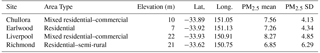
2.1 Meteorological, air quality and temporal variables
Continuous time series of hourly meteorology and PM2.5 (µg m−3) observations between January 2005 and August 2016 (inclusive) were obtained from four air quality monitoring stations (Chullora, Earlwood, Liverpool and Richmond) in the NSW Office of Environment and Heritage (OEH) network in Sydney (Fig. 1). Monitoring stations are located at varying elevations and in semi-rural, residential and commercial areas (Table 1). These four locations were chosen because they have the longest uninterrupted record of PM2.5 measurements in Sydney. Prior to 2012 PM2.5 was measured using tapered element oscillating microbalance (TEOM) systems. Since 2012 beta attenuation monitors have been used to measure PM2.5. Although there appear to be effects from instrument change, such effects are generally small if compared to the daily or hourly fluctuations in PM2.5 levels.
To compare how PM2.5 concentrations varied over daily and monthly timescales, we also obtained hourly measurements of PM10 (µg m−3), nitrogen dioxide (NO2) (parts per hundred million – pphm) and oxides of nitrogen (NOx) (pphm) from these stations. Meteorological variables included in our analyses were surface wind speed (m s−1), wind direction (∘), surface air temperature (∘C) and relative humidity (%). Hourly global solar radiation (W m−2) data were available at the Chullora station only, but were subsequently omitted as a predictive variable (see Sect. 3.3.1).
Hourly total cloud cover (okta) and mean sea level pressure (MSLP; hPa) were obtained from the Australian Bureau of Meteorology (BoM) Sydney Airport weather station (WMO station number 94767). These are included as covariates in models for the four monitoring sites. The 24 h rainfall totals (mm) were approximated for each OEH station from the BoM weather station that is nearest (Fig. 1).
Given its role in the turbulent transport of air pollutants (Seidel et al., 2010; Pal et al., 2014; Sun et al., 2015; Miao et al., 2015), we included planetary boundary layer height (PBLH) as an explanatory variable. PBLH has previously been derived from observational meteorological data by Du et al. (2013) and Lai (2015), using a method which they found was an effective estimate of the PBLH and its relationship with PM concentrations. Although direct PBLH measurements would be ideal, these are unavailable for the study domain at appropriate spatial and temporal resolutions. Hence, we derived PBLH estimates at the location of each monitoring station from a subset of the meteorological data following the method used by the above authors (Eqs. 1 and 2).
where s is a stability class that estimates lateral and vertical dispersion, t is surface air temperature and td is surface dew point temperature (approximated for the location of each station using the method proposed by Lawrence, 2005), ws is wind speed, h is wind speed altitude in m for a given monitoring station, l is the station's estimated surface roughness index, f is the Coriolis parameter in s−1, Ω is the earth's rotational speed (rad s−1) and θ is the station latitude. The stability typing scheme was based on the Pasquill–Gifford (P–G) stability categories (Turner, 1964), via a turbulence-based method using the standard deviation of the azimuth angle of the wind vector and scalar wind speed.
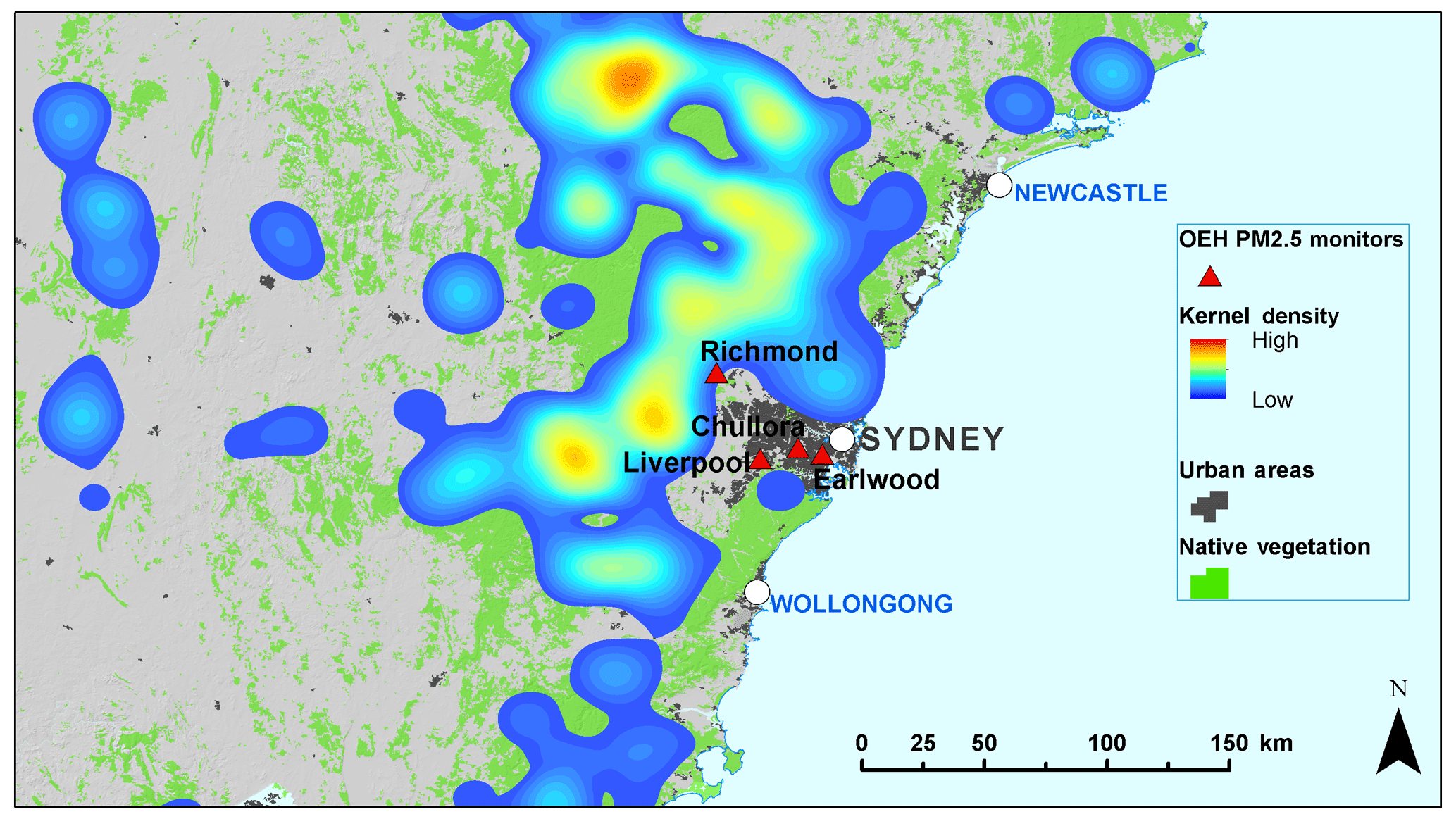
Figure 2Kernel density function (magnitude-per-unit area) for hazard reduction burns (HRBs) conducted in the vicinity of Greater Sydney (2005–2016). The warmer the colour of the kernel density surface, the more or larger HRBs that have occurred in that area. The kernel density calculation is weighted according to fire surface area.
We calculated the 24 h mean for hourly meteorological and PM2.5 measurements, where wind direction was vector-averaged (i.e. averaging the u and v wind components). Log-transformations were applied to PM2.5 and rainfall. Applying transformations to the remaining explanatory variables did not greatly reduce heterogeneity.
Temporal variables trialled for inclusion in analyses included day of the year, weekday, week, month (all representing different seasonal terms) and year (because air quality varies from year to year). A Julian date variable was incorporated to represent the longer-term trend in PM2.5 concentrations.
2.2 Burns
Historical records of HRBs conducted between January 2005 and August 2016 in NSW were obtained from the NSW Rural Fire Service (RFS), the firefighting agency responsible for the general administration of HRBs. There were a total of 9200 fire polygons in this data set prior to data conditioning (see Sect. 3). HRBs are conducted predominantly in autumn (months of March to May in the Southern Hemisphere) and spring (September to November), and often at weekends, typically, with burns lit in the early morning. Most historical HRBs have occurred to the west and north-west of Sydney (Fig. 2). Additional predictive variables derived from the HRB data (all daily values) were total number of burns, total burn surface area (ha), median burn elevation (m), median fire duration (days) and median fire distance from the geographic centre of the monitoring stations (km).
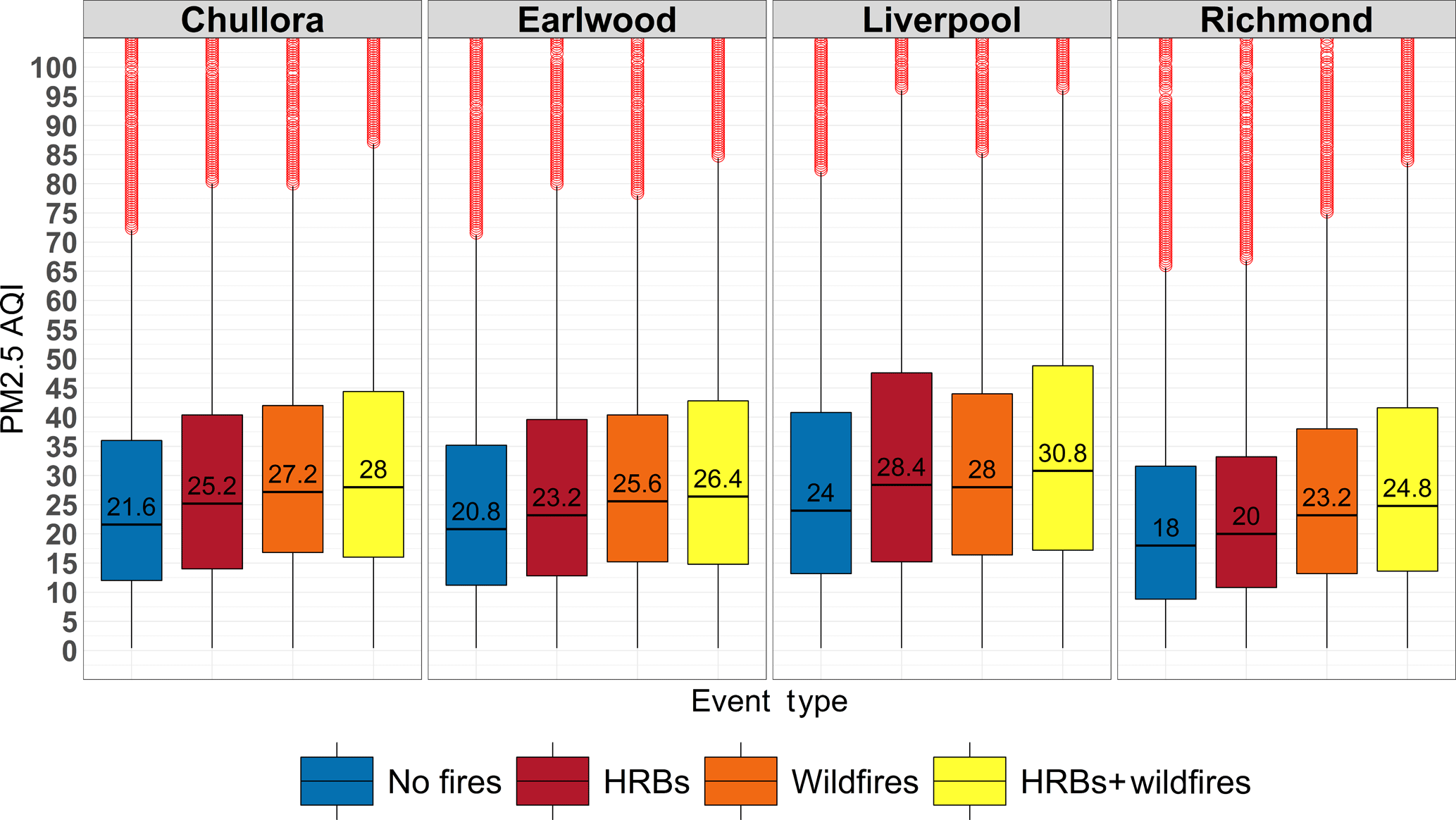
Figure 3Box plots showing the variation in PM2.5 air quality index values (AQIs) at four measurement sites in Sydney between 2011 and 2016 during days when there were no fires (neither hazard reduction burns (HRBs) or wildfires), days when only HRBs occurred without coincident wildfires, days when wildfires occurred without coincident HRBs, and days with concurrent HRBs and wildfires. Horizontal black lines on box plots are median PM2.5 AQIs, and their corresponding values are shown above these lines. Red circles are outliers.
It is important to note that other potential sources of PM2.5 emissions in Sydney include motor vehicles, soil erosion and occasional dust storms. Use of domestic wood-fired heaters can also make a substantial contribution to PM2.5 concentrations during winter months (June to August), which is when HRBs are generally not conducted. However, between 2011 and 2016, average PM2.5 air quality index (AQI) values were higher on days when either HRBs or wildfires occurred relative to days when there were no fires (Fig. 3).
3.1 Statistical approach: generalised additive mixed models
Generalised additive models (GAMs) (Hastie and Tibshirani, 1990) offer an appropriate approach with respect to air quality research because relationships between covariates are often non-linear, an issue which can be addressed within the GAM framework. In addition to the seasonal pattern of hazard reduction burning, PM2.5 concentrations in Sydney also show daily, monthly, seasonal and annual variation. Adding terms to a GAM to account for these temporal variations fails to deal with residual autocorrelation completely, as is evident in the autocorrelation function (ACF) of the residuals (Fig. S1 in the Supplement). Given the residual autocorrelation and non-independence of the data, we used a generalised additive mixed model (GAMM) approach to take account of the seasonal variation and trends in the data. GAMMs can combine fixed and random effects and enable temporal autocorrelation to be modelled explicitly (Wood, 2006). We assumed a Gaussian distribution and used a log link function. Cubic regression splines were used for all predictors except wind direction and day of year, which used cyclic cubic regression splines, because there should be no discontinuity between values at their end points. Experimenting with alternative smooth classes did not drastically affect model results or diagnostics. Smoothing parameters were chosen via restricted maximum likelihood (REML). We implemented GAMMs with a temporal residual autocorrelation structure of order 1 (AR-1). More complex structures (e.g. autoregressive moving average models; ARMAs) of varying order or moving average parameters produced marginally higher Akaike information criteria (AICs) (e.g. mean = 259.6) than models with AR-1 autocorrelation (mean AIC = 259.02). Omitting a correlation structure entirely produced the largest AICs (mean AIC = 279.5). In all cases, the AR models for the residuals were nested within 1 month (nesting within weeks and years was also trialled, but produced higher AICs). Autocorrelation plots obtained by applying the GAMMs using the AR-1 structure showed that short-term residual autocorrelation in the residuals had been removed relative to using GAMs (Figs. S1–S2).
3.2 PM2.5 trend estimates, monthly and daily means
We first used the GAMM framework to estimate the annual trend in the weekly mean concentrations of PM2.5 for 2005–2015, split by season, with Julian day as the only predictor. Monthly and daily mean PM2.5, PM10, NO2 and NOx concentrations for all years were also compared to assess how concentrations of each pollutant varied with these timescales. The latter analyses were performed using R software for statistical computing (R Development Core Team, 2015) and the “openair” package (Carslaw and Ropkins, 2012). The annual trend and subsequent statistical analyses described below were performed using R software and packages “mgcv” (Wood, 2011) and “nlme” (Pinheiro et al., 2017).
3.3 Identifying the meteorological and burn variables related to elevated PM2.5
To assess how PM2.5 concentrations vary in relation to the meteorological, burn and temporal variables, the GAMMs were applied to each monitoring site separately and focused on the period January 2011–August 2016. There were comparatively fewer HRBs conducted prior to 2011, hence the choice of this time frame. For each station, we split the data into two subsets: (1) for all days when HRBs were conducted and the PM2.5 concentration was less than the median PM2.5 concentration for the location in question, “low pollution days”; (2) for all HRB days when the PM2.5 concentration was greater than the median value for the location in question, “high pollution days” (the minimum/maximum number of observations in each low/high subset was in the range 179–189). The time series were conditioned in this manner to better characterise the differences in covariate behaviours between burn days when pollution remains low versus burn days and elevated PM2.5. Since our focus is specifically on PM2.5 concentrations during HRBs, days when wildfires had occurred were excluded.
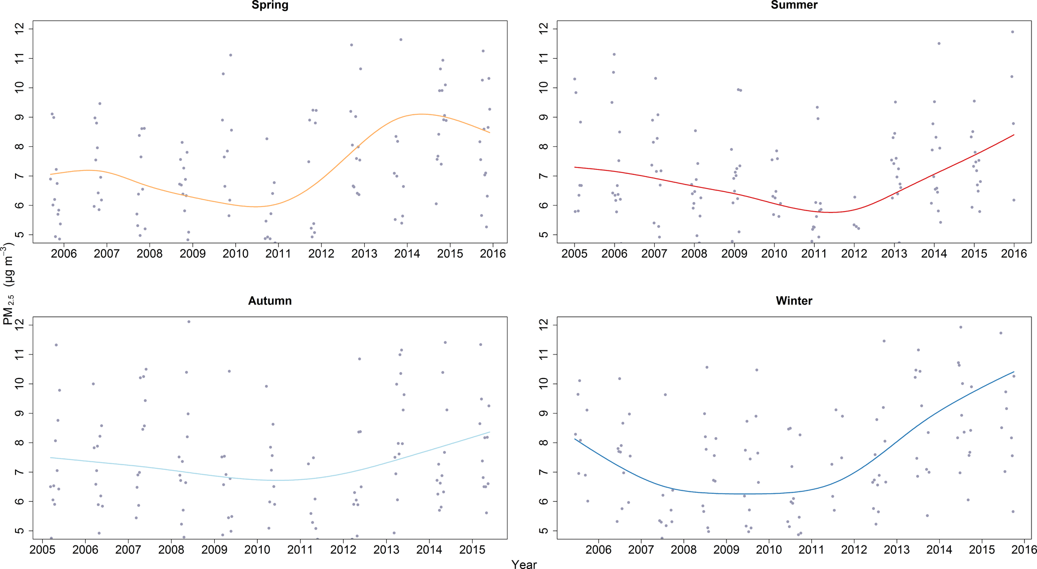
Figure 4Annual trends in the weekly mean concentrations of PM2.5 in Sydney, split by season for 2005–2015.
Model selection
Using the GAMM framework described above, we started with a model where the fixed component included all predictive variables. We used variance inflation factors (VIFs) to test variables for collinearity (Zuur et al., 2010). We sequentially dropped covariates with the highest VIF and recalculated the VIFs, repeating this process until all VIFs were smaller than a threshold of 3.5. This VIF threshold was selected as a compromise between the thresholds of 3 and 10 stipulated in Zuur et al. (2010). Following this process, explanatory variables were dropped from the initial model if they were not statistically significant in any case. As a result, global solar radiation, relative humidity, burn elevation, burn duration, day of the year, weekday, week and year were excluded. An intermediate model included HRB distance as a covariate. Exploratory GAMM analyses using this model configuration revealed that on average, beyond a distance of ca. 300 km, the influence of prescribed burns on PM2.5 concentrations at the target locations was negligible (Fig. S3). Subsequent models excluded burn distance and burns > 300 km from the geographic mean centre of the monitoring stations. Hence, the fixed component of our optimal model used the following predictors: PBLH, MSLP, temperature, total cloud cover, rainfall, wind speed, wind direction, number of burns per day, total area burnt per day and Julian day.
3.4 Diurnal variation in relation to elevated PM2.5
Meteorological covariates relevant to high PM2.5 concentrations were identified via the GAMMs based on criteria of statistical significance at more than one location, or where the influence of covariates on PM2.5 showed a marked distinction between pollution conditions. We then used the hourly meteorological data for these select covariates to compare their mean diurnal variation on burn days with low versus high pollution. The 95 % confidence intervals of these diurnal means were calculated using bootstrap re-sampling with 1000 replicates.
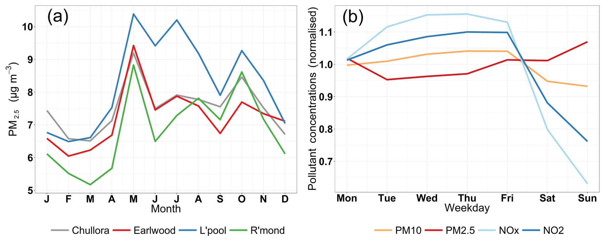
Figure 5Mean monthly PM2.5 concentrations for the period 2005 to August 2016 at four air quality monitoring sites in Greater Sydney (a). Southern Hemisphere seasons are summer (DJF), autumn (MAM), winter (JJA) and spring (SON). Mean daily normalised concentrations of PM2.5 compared to the variations of PM10, NO2 and NOx (b).
Table 2Adjusted R2, F and p values for the smoothers of the optimal generalised additive mixed models (GAMMs) applied to each monitoring site on days when hazard reduction burns occurred and with the data split into low and high air pollution conditions.
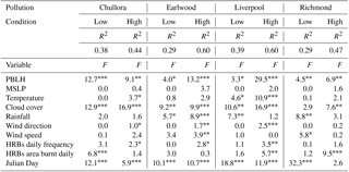
Asterisks denote statistical significance: ; ; .
4.1 Temporal variation in PM2.5 concentrations
There is an increasing inter-annual trend in weekly mean PM2.5 concentrations in all seasons during 2011 to 2015, especially in summer and winter (Fig. 4). Mean PM2.5 concentrations range from 6 to 10 µg m−3. Mean monthly PM2.5 averaged over all years shows increasing concentrations from early autumn (March), peaking in May, then decreasing towards the end of winter, before increasing again from early spring (Fig. 5a). Notably, mean daily PM2.5 concentrations (averaged over all years) are higher at weekends relative to other pollutants (PM10, NO2 and NOx; Fig. 5b).
4.2 Meteorological and burn variables related to PM2.5
Adjusted R2 values for high pollution models were between 0.44 and 0.60, and between 0.29 and 0.39 for the low pollution models (Table 2). PBLH and total cloud cover were the most consistent predictors of elevated PM2.5 during HRBs (Table 2). On high pollution days, PBLH had a statistically significant, negative influence on predicted PM2.5 concentrations at all locations (Fig. 6). This influence was generally more linear on high pollution days, relative to low pollution days. Notably, fitted curves for PM2.5–PBLH were steeper at lower altitudes (< 800 m) in the high pollution condition. Cloud cover had a negative influence on predicted PM2.5 concentrations that was significant in all but one case (Table 2), though fitted curves do not appear to differ noticeably between pollution conditions (Fig. 7). Although temperature and wind speed showed a more variable pattern of statistical significance (Table 2), they exhibited marked differences in behaviour between low and high pollution days. During high pollution, temperature typically had a negative, curvilinear influence on fitted PM2.5 values (Fig. 8). This negative influence flattens or reverses at temperatures > 20 ∘C. In contrast, the PM2.5–temperature relationship was weak and linear during low pollution days. Wind speed had a significant influence on PM2.5 only at Earlwood and Richmond (Table 2). During low pollution days, this association is negative at most locations. During high pollution conditions at Chullora and Earwood, there is a positive influence on PM2.5 at low wind speeds which reverses at speeds above ca. 2 m s−1 (Fig. S7). During HRBs and high pollution, wind direction curves show peaks between approximately 250 and 310∘ at Chullora, Earlwood and Liverpool (south-westerly to north-westerly flows) (Fig. 9). Earlwood frequently experiences north-westerly flows during spring, autumn and winter, whilst south-westerly flows are common during the same seasons at Liverpool (Fig. S4).
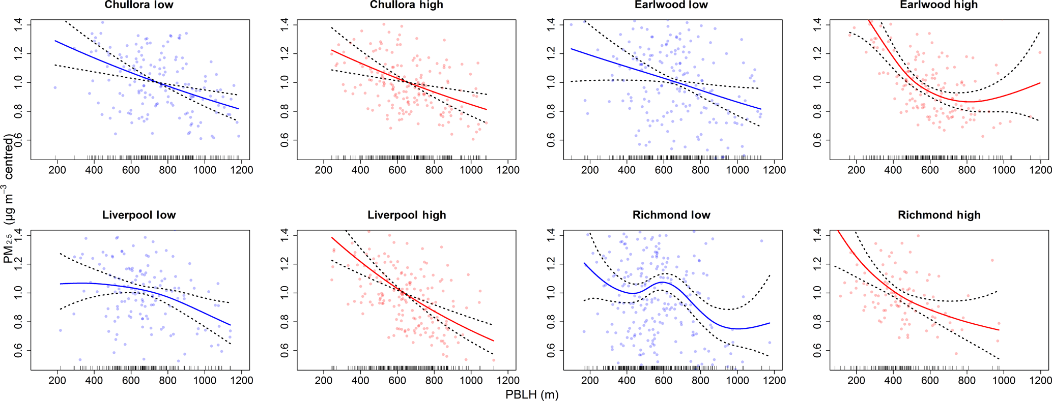
Figure 6The contribution by the planetary boundary layer height (PBLH) component of the generalised additive mixed model (GAMM) linear predictor to fitted PM2.5 values (µg m−3, centred). The solid lines are the fitted curves. Dotted lines are 95 % confidence bands. Dots are partial residuals.
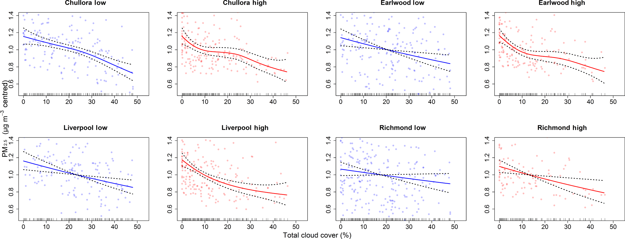
Figure 7The contribution by the cloud cover component of the GAMM linear predictor to fitted PM2.5 values (µg m−3, centred). The solid lines are the fitted curves. Dotted lines are 95 % confidence bands. Dots are partial residuals.
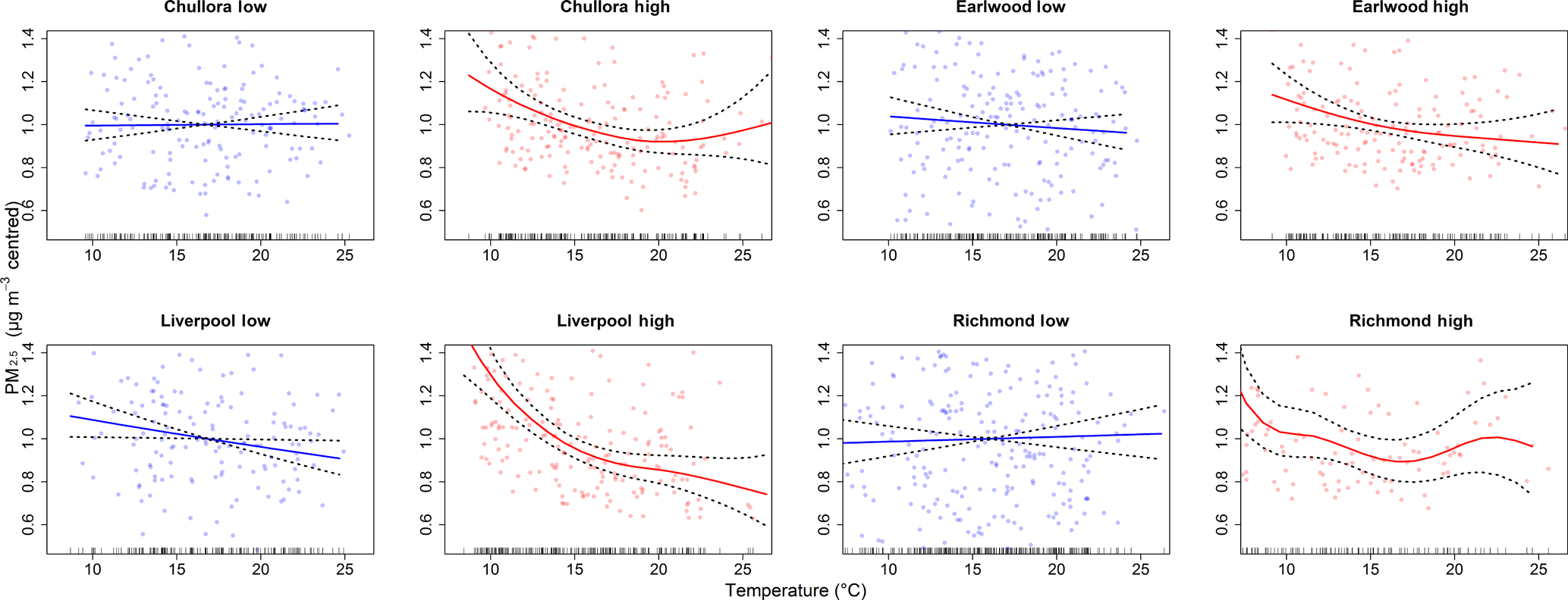
Figure 8The contribution by the temperature component of the GAMM linear predictor to fitted PM2.5 values (µg m−3, centred).
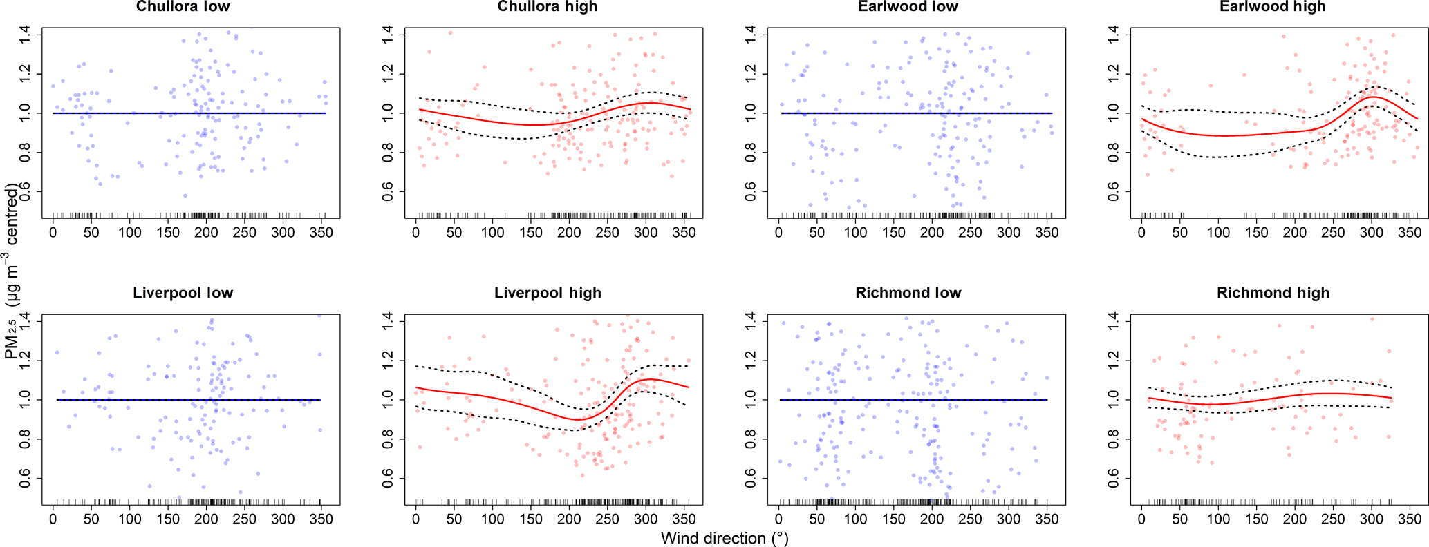
Figure 9The contribution by the wind direction component of the GAMM linear predictor to fitted PM2.5 values (µg m−3, centred).
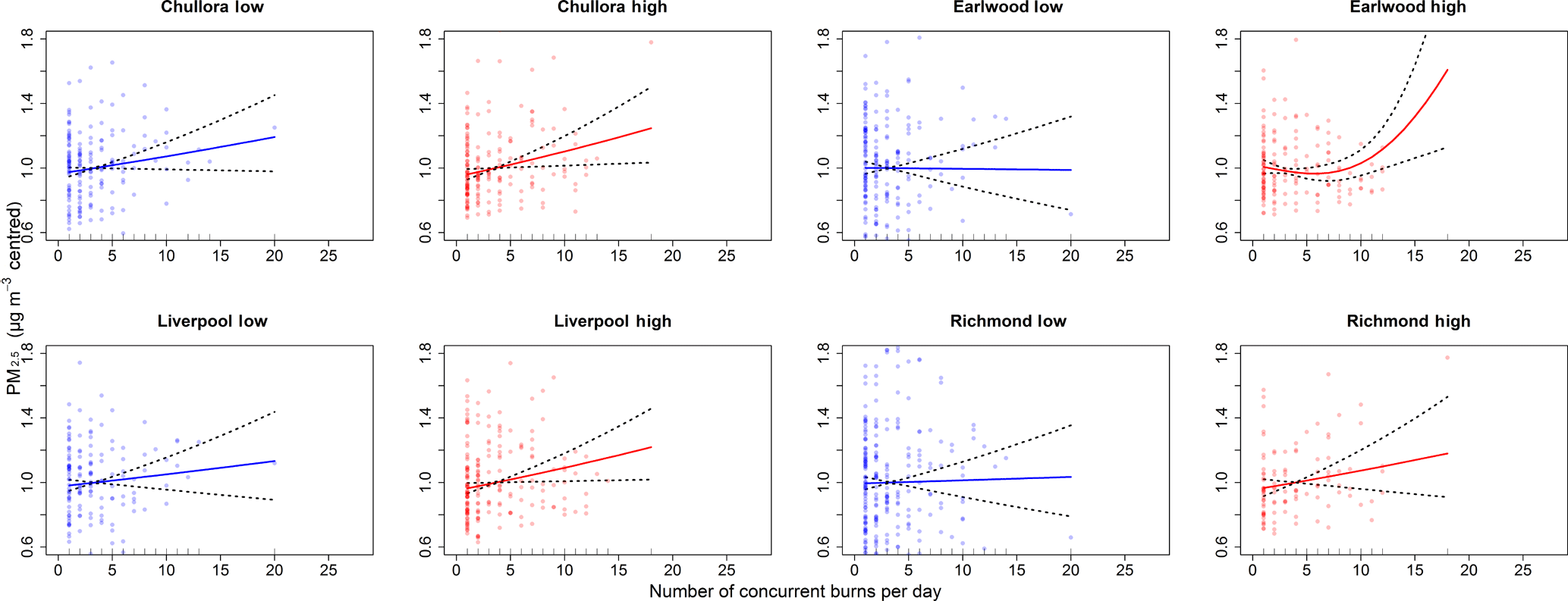
Figure 10The contribution by the hazard reduction burn (HRB) daily frequency (number of concurrent burns per day) component of the GAMM linear predictor to fitted PM2.5 values (µg m−3, centred).
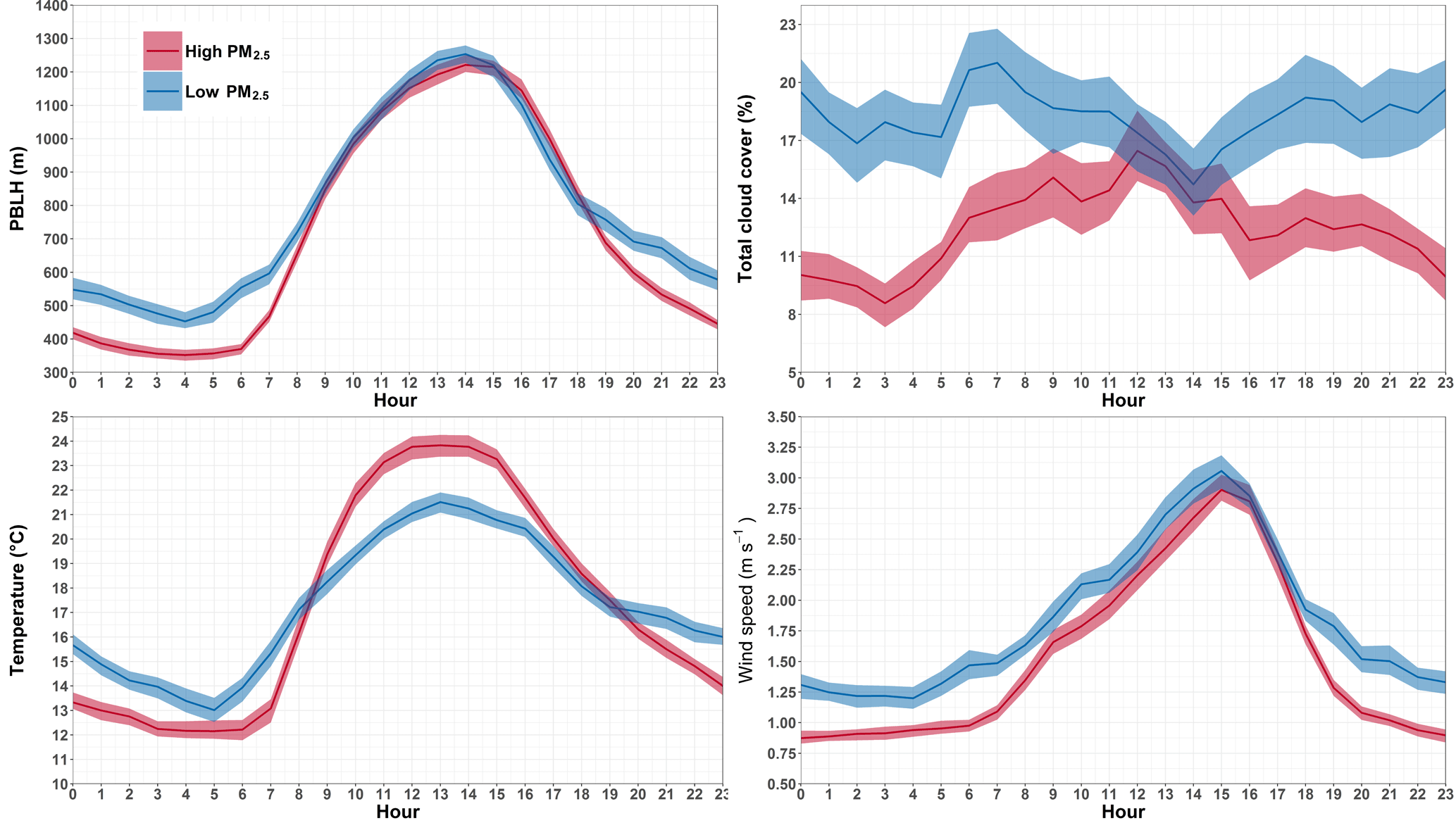
Figure 11Mean diurnal variation of hourly PBLH, total cloud cover, temperature and wind speed for low versus high PM2.5 pollution during HRBs at Liverpool, Sydney (see Figs. S8–S10 for other stations). Shading represents the 95 % confidence intervals of the means.
The remaining meteorological predictors either did not show marked differences between pollution conditions or were statistically significant in only one instance. Rainfall generally had a negative influence on PM2.5 during HRBs (Fig. S5). MSLP had a positive association with higher PM2.5 concentrations during low and high pollution (Fig. S6), though this association was only significant during high pollution at Richmond (Table 2).
HRB frequency had a significant and positive influence on PM2.5 only for the high pollution condition at Chullora, Earlwood and Liverpool (Table 2 and Fig. 10). The association between burn area and PM2.5 during high pollution was significant at Liverpool and Richmond only. The influence of Julian day on PM2.5 showed significant non-linear, increasing trends in all instances.
4.3 Differences in covariate behaviours on HRB days with low versus high PM2.5
Having identified the most informative and consistent meteorological predictors using the GAMMs, we assessed their mean diurnal variation during the occurrence of HRBs and low versus high PM2.5 pollution in the following sections.
4.3.1 PBLH
Taking Liverpool as an example, between 00:00 and 07:00 LT during low pollution days when HRBs have occurred, the PBLH is on average 100–200 m higher than during high pollution days (Fig. 11; see Figs. S8–S10 for the other monitoring stations). From late morning (ca. 10:00 LT) until early evening (ca. 19:00 LT), the PBLH altitudes of both PM2.5 conditions are very similar, but after 19:00 LT the PBLH is again higher during low pollution.
4.3.2 Total cloud cover
During HRBs, mean diurnal variation of cloud cover is between 2 and 7 % greater during the mornings and evenings of low pollution, compared to high pollution days (Fig. 11). In contrast, there is minimal difference in cloud cover during the early afternoon of both conditions.
4.3.3 Temperature
The temperature is 1–6 ∘C warmer between 00:00–08:00 LT and 20:00–23:00 LT during HRBs and low PM2.5, in comparison to burns coinciding with high pollution (Fig. 11). However, there is a clear reversal in this trend from mid-morning to late afternoon during burns and high PM2.5 when mean temperature is several degrees warmer than during HRBs and low pollution.
4.3.4 Wind speed
Mean diurnal wind speed is approximately 0.5 m s−1 higher in the mornings and after 18:00 LT during burns and low air pollution in comparison to speeds during high PM2.5 (Fig. 11). In contrast, there is a minimal difference in wind speeds between 12:00 and 18:00 LT.
Air quality in Sydney is generally good. On the occasions when it is poor, atmospheric particulates are the principal cause, and HRBs are potentially one source of high particulate emissions. Sydney's population is projected to increase (∼ 63 %) to over 8 million by 2061 (ABS, 2013), with much of the expansion occurring at the urban–bushland transition. Even if air quality remains stable, these demographic changes will increase exposure to particulate pollution. However, we observed increasing annual trends in PM2.5 concentrations. In addition, projected decreases in future rainfall (Dai, 2013) and increases in fire danger weather are likely to increase fire activity and lengthen the fire season (Bradstock et al., 2014), thus amplifying fire-related particulate emissions. Changes in measurement instrumentation have a potential for introducing systematic biases in these annual PM2.5 trends. Recently, based on the high correlation among beta attenuation monitors, PM2.5 measurements and long-term nephelometer visibility measurements at each monitoring site, the NSW Government (2016, 2017a, b) reconstructed a more consistent annual average PM2.5 time series. Their results also showed a tendency of increasing annual PM2.5 levels near 2011–2012 in some Sydney subregions, as is consistent with the results from this study. Moreover, our study also indicates that the trends start increasing from 2011 during spring and winter, which pre-dates the instrumentation change. These results suggest that the instrumentation changes that occurred in 2012 are likely to have had minimal impact on the trend analysis reported in this analysis.
Relative to other pollutants such as NOx and NO2, PM2.5 concentrations are higher at weekends. PM2.5 concentrations also start increasing in autumn with peaks in winter and spring. These patterns may reflect the timing of HRB occurrences, which occur mainly in autumn, spring and at weekends, though there is also increased domestic wood-fired heating during winter. Consequently, conducting multiple, concurrent HRBs during these periods might exacerbate PM2.5 concentrations that are already high relative to baseline.
PM2.5 concentrations tend to be dominated by organic matter (57 %) during peak HRB periods in autumn. There is also contribution, in order of apportion, from elemental carbon, inorganic aerosol and sea salt. This compares to summer months when sea salt plays a larger role, with organic matter making up just 34 % (Cope et al., 2014). Other days where national PM2.5 concentration standards have been exceeded have been attributed to wildfires and dust storms. PM2.5 concentrations also tend to be higher across the Sydney basin during winter due to smoke from wood fire heaters used for residential heating; however, exceedances of standards due to these emissions are rare (EPA, 2015).
5.1 Primary covariates affecting PM2.5 and how they differ during low and high pollution
PBLH was the most consistent meteorological predictor of PM2.5. It had a significant, negative influence on PM2.5 at all locations during HRBs and “high pollution days”. There was a marked difference in mean diurnal mixed layer heights between low and high pollution conditions in the early morning (00:00–07:00 LT) and from 20:00 to 23:00 LT, with the PBLH being approximately 100–200 m lower at these times during HRBs and high PM2.5. During these two time periods whilst the PBLH is low, mean cloud cover, temperature and wind speeds are also lower relative to their magnitudes at corresponding times during low pollution. Essentially, these early hours of cold, stable conditions with minimal turbulence (i.e. conditions that are conducive to temperature inversions) prevent the dilution of PM2.5. These subdued conditions often coincide with the night time–early morning westerly cold drainage flows and low mixing heights (inhibiting vertical dispersion), leading to the build-up of PM2.5 during mornings (Lu and Turco, 1995; Hart et al., 2006; Jiang et al., 2016b). These pollution-conducive conditions are similar to those identified in Jiang et al. (2016a) as being related to a ridge of high pressure extending across eastern Australia, resulting in light north-westerly winds. These synoptically driven flows, although light, tend to enhance nocturnal drainage flows, inhibit afternoon sea breeze formation and allow the transportation of pollutants across the Sydney basin to the coast. There is also a large difference in mean diurnal temperatures between low and high pollution conditions from late morning to early evening, with temperatures 3–4 ∘C warmer during high pollution. During warmer daytime conditions, PM2.5 can be potentially higher without fire events, for instance, because these conditions tend to be coincident with increased precursor emissions and generation of secondary organic aerosols in the air. Furthermore, the fact that early morning and late evening temperatures tend to be lower during high pollution conditions may indicate the presence of temperature inversions which hinder atmospheric convection, leading to the collection of particulates that cannot be lifted from the surface. Cold morning temperatures can also result in stronger drainage flows into the Sydney basin. Consequently, if HRBs are being conducted during early mornings in the hills and mountains to the west of Sydney, this could result in the dispersion of particles from such sources, possibly into populated areas.
These findings indicate how the timing of HRBs can be altered to reduce their air pollution impacts in Sydney. Conducting HRBs when the PBLH is forecast to be higher ought to help reduce their air quality impacts in Sydney. More specifically, conducting HRBs later in the morning (for example by a matter of hours) is one way of potentially reducing HRB air quality impacts, because the PBLH generally starts increasing rapidly in height from 07:00 until 12:00 LT. Fires conducted early in the morning when the PBLH is at its lowest and temperatures are cool will promote effects such as fire smoke residing near ground level. One constraint concerning later burn times is that wind speed typically increases as the day progresses. However, the maximum mean diurnal wind speed was approximately 3 m s−1 and occurred at 15:00 LT. This is considerably lower than the RFS's upper-limit of 5.56 m s−1 for conducting safe HRBs (Plucinski and Cruz, 2015). An additional caution for conducting burns later in the afternoon is that onshore coastal breezes can develop during afternoons. The optimal timing of burns will also be dependent on other factors such as burn intensity, lighting method, fuel–soil moisture and geographic location.
There was a negative association between cloud cover and PM2.5 levels. It is possible that fire agencies conduct fewer HRBs during cloudy conditions in case of rain. Rainfall (if any) can also scavenge PM pollution out of the air. However, cloudless skies are also associated with high pressure systems, and therefore cool air descending, resulting in a stable calm atmosphere and low PBLH that is not conducive to pollutant dispersion.
Although there were similarities in the influence of covariates between locations, these associations often varied spatially. For example, mean diurnal PBLH and temperature were lower at Richmond in the early morning and at night in comparison to the other locations (Fig. S10). Richmond is further inland than the other monitoring sites and is thus closer to the mountain range to the west of Sydney. The insights gained into the spatial variation in the behaviour of covariates can support efforts to create location-specific particulate pollution forecasts.
The north-westerly signal apparent for three of four locations during HRBs and high pollution may reflect the fact that, overall, the majority of burns are conducted to the west, north and north-west of Sydney (Fig. 2). From a management perspective, comparatively greater attention might be devoted to adapting burn operations in these regions. In the case of Richmond (where wind direction did not have a statistically significant influence), one possible explanation is that the daily vector-averaging applied to the wind data has smoothed out the signal associated with diurnal changes in wind directions (and speeds), e.g. between drainage flow and sea breezes. Thus, to some degree, the signal of wind influence may be suppressed in this case. Another contributing factor could be Richmond's generally closer proximity to local burns. Also, its geographic location is quite different to that of the other monitoring sites; it is further inland than the other sites and is thus closer to the mountain range to the west of Sydney.
Using a different analysis approach, Price et al. (2012) found that the optimum radius of influence of landscape fires on PM2.5 was 100 km for Sydney. We found that whilst close-proximity fires influenced air quality, fires up to approximately 300 km from monitoring stations also potentially influenced PM2.5. Longer-range exposures on regional scales, particularly from multiple HRBs in an air shed can impact communities at considerable distance under certain atmospheric transport conditions (e.g. Liu et al., 2009).
Multiple concurrent burns are more likely to adversely affect air quality in Sydney, as indicated by the significant, positive influence of the number of concurrent HRBs on PM2.5 during high pollution days at all locations except Richmond. In general, greater numbers of concurrent burns within a given air shed are likely to result in greater quantities of particulate emissions. The area of these burns would also determine the amount of particulate emissions generated. HRB total area per day was a statistically significant predictor at two locations (Liverpool and Richmond). There are several possible explanations for the fact that burn daily frequency and area are not significant predictors at all locations. There will be some noise in total PM2.5 concentrations contributed by other emission sources, and this will vary with location. For example, Richmond differs from the other monitoring sites in that it is near agricultural land, and so emission sources like soil erosion and fertiliser use will introduce noise at this location. Investigating the relationships between burnt area and fire-related tracer species to reduce the noise in total concentrations contributed by other sources could be attempted in future work. There are also uncertainties regarding how accurately the area actually burnt was recorded within some polygons representing HRBs. In particular, to date it has been difficult to obtain timely and accurate estimates of the actual area burnt. Moreover, larger burns are often further away from the urban centres chosen, and are less frequent than smaller burns. In contrast, moderate to small burns are more frequent and often scattered along the urban fringes (rather than confined to one location or direction) and thus have a larger effect on the overall air quality within urban centres. Transport of smoke is also determined by interactions between basin topography and local or synoptic wind conditions. However, the interaction between mesoscale geography and meteorological variables is a factor that could not be easily accounted for in the present study (i.e. each site is located in a different location, therefore each has differing topography and land use type).
Fine particulate concentrations are increasing in Sydney, and given projected increases in fire danger weather, intensification in fire activity is expected to further amplify fire-related PM2.5 emissions. We identified the key meteorological factors linked to elevated PM2.5 during HRBs. In particular, diurnal variation of the PBLH, cloud cover, temperature and wind speed have a pervasive influence on PM2.5 concentrations, with these factors being more variable and higher in magnitude during the mornings and evenings of HRB days when PM2.5 remains low. These findings indicate how the timing of HRBs can be altered to minimise pollution impacts. They can also support locality-specific forecasts of the air quality impacts of burns in Sydney and potentially other locations globally. In addition to mitigating wildfire risk, HRBs are used globally for forest management, farming, prairie restoration and greenhouse gas abatement. Future research should incorporate more sophisticated fire characteristics such as plume height and fuel moisture into analyses, and also consider the influence of climatic phenomena on particulate pollution. Synoptic features can also be incorporated into a future GAMM analysis, as well as modelling the diurnal evolution of PM2.5 pollution due to HRB occurrences.
Meteorology and air quality data were obtained from the New South Wales Office of Environment and Heritage (http://www.environment.nsw.gov.au/, New South Wales Office of Environment and Heritage, 2005–2016). Cloud cover and rainfall data were obtained from the Australian Bureau of Meteorology (http://www.bom.gov.au/, Bureau of Meteorology, 2005–2016). Data on historical burns were obtained from the New South Wales Rural Fire Service (https://www.rfs.nsw.gov.au/, New South Wales Rural Fire Service, 2005–2016).
The supplement related to this article is available online at: https://doi.org/10.5194/acp-18-6585-2018-supplement.
GDV, MAH and NJ conceived the research questions and aims. GDV designed and performed the analyses with contributions from all co-authors. GDV prepared the paper with contributions from all co-authors.
The authors declare that they have no conflict of interest.
This research was supported by the NSW Environmental Trust under grant
2014/RD/0147 and the NSW Office of Environment and Heritage (OEH). We thank
OEH, the Bureau of Meteorology, and the NSW Rural Fire Service NSW (NSW RFS) for providing the air
quality, meteorological and fire data used in this research. We also thank four anonymous reviewers who provided valuable feedback on this research.
Edited by: Yun Qian
Reviewed by: four
anonymous referees
ABS – Australian Bureau of Statistics: Population Projections, Australia, 2012 to 2101, Government of Australia, Canberra, 2013.
ABS – Australian Bureau of Statistics: Regional population growth, Australia, 2014–15: estimated resident population – greater capital city statistical areas, Government of Australia, Canberra, 2016.
Attiwill, P. M. and Adams, M. A.: Mega-fires, inquiries and politics in the eucalypt forests of Victoria, south-eastern Australia, Forest Ecol. Manag., 294, 45–53, https://doi.org/10.1016/j.foreco.2012.09.015, 2013.
Bradstock, R., Penman, T., Boer, M., Price, O., and Clarke, H.: Divergent responses of fire to recent warming and drying across south-eastern Australia, Glob. Change Biol., 20, 1412–1428, 10.1111/gcb.12449, 2014.
Broome, R. A., Johnstone, F. H., Horsley, J., and Morgan, G. G.: A rapid assessment of the impact of hazard reduction burning around Sydney, May 2016, Med. J. Aust., 205, 407–408, https://doi.org/10.5694/mja16.00895, 2016.
Bureau of Meteorology: Climate Data Online, available at: http://www.bom.gov.au/climate/data/index.shtml?bookmark=201 (last access: 29 November 2016), 2005–2016.
Carslaw, D. C. and Ropkins, K.: openair – An R package for air quality data analysis, Environ. Model. Softw., 27–28, 52–61, 10.1016/j.envsoft.2011.09.008, 2012.
Cohen, A. J., Ross Anderson, H., Ostro, B., Pandey, K. D., Krzyzanowski, M., Künzli, N., Gutschmidt, K., Pope, A., Romieu, I., Samet, J. M., and Smith, K.: The Global Burden of Disease Due to Outdoor Air Pollution, Jpn. J. Tox. Env. Health, 68, 1301–1307, https://doi.org/10.1080/15287390590936166, 2005.
Cope, M. E., Keywood, M. D., Emmerson, K., Galbally, I., Boast, K., Chambers, S., Cheng, M., Crumeyrolle, S., Dunne, E., Fedele, R., Gillett, R., Griffiths, A., Harnwell, J., Katzfey, J., Hess, D., Lawson, S., Milijevic, B., Molloy, S., Powell, J., Reisen, F., Ristovski, Z., Selleck, P., Ward, J., Zhang, C., and Zeng, J.: Sydney particle study – Stage II, The Centre for Australian Weather and Climate Research, 151 pp., 2014.
Dai, A. G.: Increasing drought under global warming in observations and models, Nat. Clim. Change, 3, 52–58, https://doi.org/10.1038/nclimate1633, 2013.
Du, C. L., Liu, S. Y., Yu, X., Li, X. M., Chen, C., Peng, Y., Dong, Y., Dong, Z. P., and Wang, F. Q.: Urban Boundary Layer Height Characteristics and Relationship with Particulate Matter Mass Concentrations in Xi'an, Central China, Aerosol Air Qual. Res., 13, 1598–1607, https://doi.org/10.4209/aaqr.2012.10.0274, 2013.
Dutta, R., Das, A., and Aryal, J.: Big data integration shows Australian bush-fire frequency is increasing significantly, Roy. Soc. Open Sci., 3, 150241, https://doi.org/10.1098/rsos.150241, 2016.
EPA – Environment Protection Authority: New South Wales State of the Environment 2015, EPA20150817, EPA, 240 pp., 2015.
Fernandes, P. M. and Botelho, H. S.: A review of prescribed burning effectiveness in fire hazard reduction, Int. J. Wildland Fire, 12, 117–128, https://doi.org/10.1071/wf02042, 2003.
Flannigan, M., Cantin, A. S., de Groot, W. J., Wotton, M., Newbery, A., and Gowman, L. M.: Global wildland fire season severity in the 21st century, Forest Ecol. Manag., 294, 54–61, https://doi.org/10.1016/j.foreco.2012.10.022, 2013.
Haikerwal, A., Akram, M., Sim, M. R., Meyer, M., Abramson, M. J., and Dennekamp, M.: Fine particulate matter (PM2.5) exposure during a prolonged wildfire period and emergency department visits for asthma, Respirology, 21, 88–94, https://doi.org/10.1111/resp.12613, 2016.
Hart, M., De Dear, R., and Hyde, R.: A synoptic climatology of tropospheric ozone episodes in Sydney, Australia, Int. J. Climatol., 26, 1635–1649, https://doi.org/10.1002/joc.1332, 2006.
Hastie, T. J. and Tibshirani, R. J.: Generalized Additive Models, Taylor & Francis, 1990.
Hyde, R., Malfroy, H. R., Heggie, A. C., and Hawke, G. S.: The western basin experiment. A study of nocturnal drainage flows in the Sydney basin and their implications for future planning, Report to the NSW State Pollution Control Commission, School of Earth Sciences, Macquarie University, Sydney Australia, 1980.
Jalaludin, B., Morgan, G., Lincoln, D., Sheppeard, V., Simpson, R., and Corbett, S.: Associations between ambient air pollution and daily emergency department attendances for cardiovascular disease in the elderly (65+years), Sydney, Australia, J. Expo. Sci. Environ. Epidemiol., 16, 225–237, https://doi.org/10.1038/sj.jea.7500451, 2006.
Jalaludin, B., Khalaj, B., Sheppeard, V., and Morgan, G.: Air pollution and ED visits for asthma in Australian children: a case-crossover analysis, Int. Arch. Occup. Environ. Health, 81, 967–974, https://doi.org/10.1007/s00420-007-0290-0, 2008.
Jiang, N., Betts, A., and Riley, M.: Summarising climate and air quality (ozone) data on self-organising maps: a Sydney case study, Environ. Monit. Assess., 188, 103 pp., https://doi.org/10.1007/s10661-016-5113-x, 2016a.
Jiang, N., Scorgie, Y., Hart, M., Riley, M. L., Crawford, J., Beggs, P. J., Edwards, G. C., Chang, L., Salter, D., and Di Virgilio, G.: Visualising the relationships between synoptic circulation type and air quality in Sydney, a subtropical coastal-basin environment, Int. J. Climatol., 37, 1211–1228, https://doi.org/10.1002/joc.4770, 2016b.
Johnston, F., Hanigan, I., Henderson, S., Morgan, G., and Bowman, D.: Extreme air pollution events from bushfires and dust storms and their association with mortality in Sydney, Australia 1994–2007, Environ. Res., 111, 811–816, https://doi.org/10.1016/j.envres.2011.05.007, 2011.
Johnston, F., Purdie, S., Jalaludin, B., Martin, K. L., Henderson, S. B., and Morgan, G. G.: Air pollution events from forest fires and emergency department attendances in Sydney, Australia 1996–2007: a case-crossover analysis, Environ. Health, 13, 1–9, https://doi.org/10.1186/1476-069x-13-105, 2014.
Keywood, M., Kanakidou, M., Stohl, A., Dentener, F., Grassi, G., Meyer, C. P., Torseth, K., Edwards, D., Thompson, A. M., Lohmann, U., and Burrows, J.: Fire in the Air: Biomass Burning Impacts in a Changing Climate, Crit. Rev. Env. Contr., 43, 40–83, https://doi.org/10.1080/10643389.2011.604248, 2013.
Lai, L. W.: Fine particulate matter events associated with synoptic weather patterns, long-range transport paths and mixing height in the Taipei Basin, Taiwan, Atmos. Environ., 113, 50–62, https://doi.org/10.1016/j.atmosenv.2015.04.052, 2015.
Lawrence, M. G.: The Relationship between Relative Humidity and the Dewpoint Temperature in Moist Air: A Simple Conversion and Applications, B. Am. Meteorol. Soc., 86, 225–233, https://doi.org/10.1175/BAMS-86-2-225, 2005.
Liu, Y. Q., Goodrick, S., Achtemeier, G., Jackson, W. A., Qu, J. J., and Wang, W. T.: Smoke incursions into urban areas: simulation of a Georgia prescribed burn, Int. J. Wildland Fire, 18, 336–348, https://doi.org/10.1071/wf08082, 2009.
Lu, R. and Turco, R. P.: Air pollutant transport in a coastal environment, 2. 3-Dimensional simulations over Los-Angeles Basin, Atmos. Environ., 29, 1499–1518, https://doi.org/10.1016/1352-2310(95)00015-q, 1995.
Luo, L. F., Tang, Y., Zhong, S. Y., Bian, X. D., and Heilman, W. E.: Will Future Climate Favor More Erratic Wildfires in the Western United States?, J. Appl. Meteorol. Climatol., 52, 2410–2417, https://doi.org/10.1175/jamc-d-12-0317.1, 2013.
Miao, Y., Hu, X.-M., Liu, S., Qian, T., Xue, M., Zheng, Y., and Wang, S.: Seasonal variation of local atmospheric circulations and boundary layer structure in the Beijing-Tianjin-Hebei region and implications for air quality, J. Adv. Model Earth Sy., 7, 1602–1626, https://doi.org/10.1002/2015MS000522, 2015.
Morgan, G., Sheppeard, V., Khalaj, B., Ayyar, A., Lincoln, D., Jalaludin, B., Beard, J., Corbett, S., and Lumley, T.: Effects of Bushfire Smoke on Daily Mortality and Hospital Admissions in Sydney, Australia, Epidemiology, 21, 47–55, https://doi.org/10.1097/EDE.0b013e3181c15d5a, 2010.
Naeher, L. P., Brauer, M., Lipsett, M., Zelikoff, J. T., Simpson, C. D., Koenig, J. Q., and Smith, K. R.: Woodsmoke Health Effects: A Review, Inhal. Toxicol., 19, 67–106, https://doi.org/10.1080/08958370600985875, 2007.
New South Wales Office of Environment and Heritage: Hourly averages for all criterion pollutants and meteorology variables, available at: http://www.environment.nsw.gov.au/AQMS/search.htm (last access: 29 November 2016), 2005–2016.
New South Wales Rural Fire Service: Historical Hazard Reduction Burns, available at: https://www.rfs.nsw.gov.au/resources/access-to-information (last access: 28 November 2016), 2005–2016.
NSW Government: Consutlation paper: clean air for New South Wales. New South Wales Environment Protection Authority and Office of Environment and Heritage, Sydney, Australia, 2016.
NSW Government: Clean air for NSW: Air quality in NSW, Office of Environment and Heritage, Sydney, Australia, 2017a.
NSW Government: Clean air for NSW: Clear air metric, Office of Environment and Heritage, Sydney, Australia, 2017b.
OEH – Office of Environment and Heritage.: New South Wales climate change snapshot, New South Wales State Government, Sydney, 2014.
OEH – Office of Environment and Heritage: Towards Cleaner Air: New South Wales Air Quality Statement 2016, New South Wales State Government, Sydney, 2016.
Pal, S., Lee, T. R., Phelps, S., and De Wekker, S. F. J.: Impact of atmospheric boundary layer depth variability and wind reversal on the diurnal variability of aerosol concentration at a valley site, Sci. Total Environ., 496, 424–434, https://doi.org/10.1016/j.scitotenv.2014.07.067, 2014.
Pearce, J. L., Rathbun, S., Achtemeier, G., and Naeher, L. P.: Effect of distance, meteorology, and burn attributes on ground-level particulate matter emissions from prescribed fires, Atmos. Environ., 56, 203–211, https://doi.org/10.1016/j.atmosenv.2012.02.056, 2012.
Pinheiro, J., Bates, D., DebRoy, S., Sarkar, D., and R Core Team.: nlme: Linear and Nonlinear Mixed Effects Models, R package version 3.1-131, available at: https://CRAN.R-project.org/package=nlme, 2017.
Plucinski, M. P. and Cruz, M. G.: Evaluation of the Prescribed Burn Forecast Tool. CSIRO client report No EP155001, Commonwealth Scientific and Industrial Research Organisation, Canberra, Australia, 2015.
Price, O. F., Williamson, G. J., Henderson, S. B., Johnston, F., and Bowman, D.: The Relationship between Particulate Pollution Levels in Australian Cities, Meteorology, and Landscape Fire Activity Detected from MODIS Hotspots, PloS one, 7, e47327, https://doi.org/10.1371/journal.pone.0047327, 2012.
Raaschou-Nielsen, O., Andersen, Z. J., Beelen, R., Samoli, E., Stafoggia, M., Weinmayr, G., Hoffmann, B., Fischer, P., Nieuwenhuijsen, M. J., Brunekreef, B., Xun, W. W., Katsouyanni, K., Dimakopoulou, K., Sommar, J., Forsberg, B., Modig, L., Oudin, A., Oftedal, B., Schwarze, P. E., Nafstad, P., De Faire, U., Pedersen, N. L., Östenson, C.-G., Fratiglioni, L., Penell, J., Korek, M., Pershagen, G., Eriksen, K. T., Sørensen, M., Tjønneland, A., Ellermann, T., Eeftens, M., Peeters, P. H., Meliefste, K., Wang, M., Bueno-de-Mesquita, B., Key, T. J., de Hoogh, K., Concin, H., Nagel, G., Vilier, A., Grioni, S., Krogh, V., Tsai, M.-Y., Ricceri, F., Sacerdote, C., Galassi, C., Migliore, E., Ranzi, A., Cesaroni, G., Badaloni, C., Forastiere, F., Tamayo, I., Amiano, P., Dorronsoro, M., Trichopoulou, A., Bamia, C., Vineis, P., and Hoek, G.: Air pollution and lung cancer incidence in 17 European cohorts: prospective analyses from the European Study of Cohorts for Air Pollution Effects (ESCAPE), The Lancet Oncology, 14, 813–822, https://doi.org/10.1016/S1470-2045(13)70279-1, 2013.
R Development Core Team: R: A language and environment for statistical computing, R Foundation for Statistical Computing, 2015.
RFS – Rural Fire Service: NSW RFS Annual Report 2014/15, State of New South Wales, Sydney, Australia, 2015.
Seidel, D. J., Ao, C. O., and Li, K.: Estimating climatological planetary boundary layer heights from radiosonde observations: Comparison of methods and uncertainty analysis, J. Geophys. Res.-Atmos., 115, D16113, https://doi.org/10.1029/2009jd013680, 2010.
Sun, Y., Du, W., Wang, Q., Zhang, Q., Chen, C., Chen, Y., Chen, Z., Fu, P., Wang, Z., Gao, Z., and Worsnop, D. R.: Real-Time Characterization of Aerosol Particle Composition above the Urban Canopy in Beijing: Insights into the Interactions between the Atmospheric Boundary Layer and Aerosol Chemistry, Environ. Sci. Technol., 49, 11340–11347, https://doi.org/10.1021/acs.est.5b02373, 2015.
Turner, D. B.: A Diffusion Model for an Urban Area, J. Appl. Meteorol., 3, 83–91, https://doi.org/10.1175/1520-0450(1964)003<0083:ADMFAU>2.0.CO;2, 1964.
Weise, D. R., Johnson, T. J., and Reardon, J.: Particulate and trace gas emissions from prescribed burns in southeastern US fuel types: Summary of a 5-year project, Fire Saf. J., 74, 71–81, https://doi.org/10.1016/j.firesaf.2015.02.016, 2015.
Westerling, A. L.: Increasing western US forest wildfire activity: sensitivity to changes in the timing of spring, Philos. T. Roy. Soc. B, 371, 20150178, https://doi.org/10.1098/rstb.2015.0178, 2016.
Westerling, A. L., Hidalgo, H. G., Cayan, D. R., and Swetnam, T. W.: Warming and Earlier Spring Increase Western U.S. Forest Wildfire Activity, Science, 313, 940–943, https://doi.org/10.1126/science.1128834, 2006.
Wood, S. N.: Generalized Additive Models: An Introduction with R, Chapman and Hall/CRC, London/Boca Raton, FL, 2006.
Wood, S. N.: Fast stable restricted maximum likelihood and marginal likelihood estimation of semiparametric generalized linear models, J. R. Stat. Soc. B, 73, 3–36, https://doi.org/10.1111/j.1467-9868.2010.00749.x, 2011.
Zuur, A. F., Ieno, E. N., and Elphick, C. S.: A protocol for data exploration to avoid common statistical problems, Methods Ecol. Evol., 1, 3–14, https://doi.org/10.1111/j.2041-210X.2009.00001.x, 2010.