the Creative Commons Attribution 4.0 License.
the Creative Commons Attribution 4.0 License.
 | 07 May 2018
Representativeness of single lidar stations for zonally averaged ozone profiles, their trends and attribution to proxies
Christos Zerefos
John Kapsomenakis
Kostas Eleftheratos
Kleareti Tourpali
Irina Petropavlovskikh
Daan Hubert
Sophie Godin-Beekmann
Wolfgang Steinbrecht
Stacey Frith
Viktoria Sofieva
Birgit Hassler
This paper is focusing on the representativeness of single lidar stations for zonally averaged ozone profile variations over the middle and upper stratosphere. From the lower to the upper stratosphere, ozone profiles from single or grouped lidar stations correlate well with zonal means calculated from the Solar Backscatter Ultraviolet Radiometer (SBUV) satellite overpasses. The best representativeness with significant correlation coefficients is found within ±15∘ of latitude circles north or south of any lidar station. This paper also includes a multivariate linear regression (MLR) analysis on the relative importance of proxy time series for explaining variations in the vertical ozone profiles. Studied proxies represent variability due to influences outside of the earth system (solar cycle) and within the earth system, i.e. dynamic processes (the Quasi Biennial Oscillation, QBO; the Arctic Oscillation, AO; the Antarctic Oscillation, AAO; the El Niño Southern Oscillation, ENSO), those due to volcanic aerosol (aerosol optical depth, AOD), tropopause height changes (including global warming) and those influences due to anthropogenic contributions to atmospheric chemistry (equivalent effective stratospheric chlorine, EESC). Ozone trends are estimated, with and without removal of proxies, from the total available 1980 to 2015 SBUV record. Except for the chemistry related proxy (EESC) and its orthogonal function, the removal of the other proxies does not alter the significance of the estimated long-term trends. At heights above 15 hPa an “inflection point” between 1997 and 1999 marks the end of significant negative ozone trends, followed by a recent period between 1998 and 2015 with positive ozone trends. At heights between 15 and 40 hPa the pre-1998 negative ozone trends tend to become less significant as we move towards 2015, below which the lower stratosphere ozone decline continues in agreement with findings of recent literature.


At least three recently published papers (Steinbrecht et al., 2017; Weber et al., 2018; Ball et al., 2018) show that total ozone and ozone profile trends are consistent with earlier WMO Scientific Assessment of Ozone Depletion (2014) findings. Despite the addition of four more years since WMO Scientific Assessment of Ozone Depletion (2014), Weber et al. (2018) show that for most datasets and regions the trends in total ozone, since stratospheric halogens reached their maximum around 1997, are not significantly different from zero. In the case of ozone profile trends, however, Steinbrecht et al. (2017) confirmed increasing trends in the upper stratosphere (2 hPa) as first reported in WMO Scientific Assessment of Ozone Depletion (2014). Due to improved datasets and longer records, the uncertainty in the profile trends reported by Steinbrecht et al. (2017) was reduced by a factor of 2 compared to the estimates by Harris et al. (2015). Moreover Ball et al. (2018) provided solid evidence for a continuous ozone decline in the lower stratosphere capable of offsetting ozone recovery seen at the upper layers in the stratosphere.
In this work we have analysed Solar Backscatter Ultraviolet Radiometer (SBUV; McPeters et al., 2013; Frith et al., 2017) and lidar ozone profile data from the Network for the Detection of Atmospheric Composition Change (NDACC) as part of the Long-term Ozone Trends and Uncertainties in the Stratosphere (LOTUS) project (http://igaco-o3.fmi.fi/LOTUS/index.html, last access: 2 May 2018). The project aims at providing support and input to the WMO/UNEP 2018 Ozone Assessment for a better understanding of ozone trends and their significance as a function of altitude and latitude, nearly 20 years after the peak of ozone depleting substances in the stratosphere. Among the objectives of the LOTUS initiative is the improvement of our understanding of all sources of uncertainties in estimated trends and regression methods. In this work we provide a new look at the uncertainties involved in the representativeness of single (lidar) stations for zonally averaged layer ozone. We then look at ozone trends and at the hierarchy of proxies commonly used in statistical ozone trend analyses. We try to provide a better understanding of uncertainties and to quantify the effect of stratospheric climatology and chemistry on the estimated profile trends.
2.1 Satellite data
Solar Backscatter Ultraviolet Radiometer (SBUV) version 8.6 station overpass satellite data for the period 1980–2015 have been analysed in this work. The SBUV observing system consists of a series of instruments that measure ozone profiles from the ground to the top of the atmosphere (e.g. DeLand et al., 2012; McPeters et al., 2013). Measurements are provided as partial column ozone amounts in Dobson units (DU). We have analysed ozone data for seven pressure layers as shown in Table 1.
Table 1Pressure layers in which ozone data have been analysed in this study.
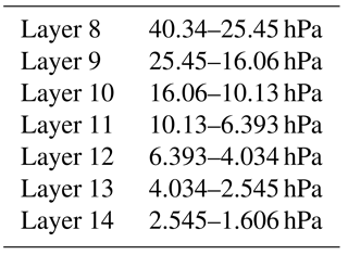
The satellite data come from all SBUV-type instruments with data availability from November 1978 to the present (see Table 2 for details). Three versions of the SBUV instrument are used in the series, but the fundamental measurement technique is the same over the evolution of the instrument from the Backscatter Ultraviolet Radiometer (BUV) to SBUV/2 (Bhartia et al., 2013). Satellite overpasses over a number of ground stations are available for each day from the web address ftp://toms.gsfc.nasa.gov/pub/sbuv/AGGREGATED/ (last access: 2 May 2018). Daily averages have been calculated by averaging the measurements from all available satellite instruments. Then monthly means were derived following the instructions provided at https://acd-ext.gsfc.nasa.gov/Data_services/merged/instruments.html (last access: 2 May 2018). Additional SBUV data used in the present work include 5∘ of latitude zonal means taken from ftp://toms.gsfc.nasa.gov/pub/MergedOzoneData/Ind_Inst_HDF/ (McPeters et al., 2013).
2.2 Lidar data
Monthly mean ozone profiles from ground-based lidar instruments were obtained by averaging daily profiles from the NDACC database at ftp://ftp.cpc.ncep.noaa.gov/ndacc/station/ (last access: 2 May 2018; De Mazière et al., 2018). Data for lidar stations with long-term measurements, namely Hohenpeißenberg (47.8∘ N, 11.0∘ E), Haute Provence (43.9∘ N, 5.7∘ E) and Table Mountain (34.4∘ N, 117.7∘ W) in the northern mid-latitudes; Mauna Loa (19.5∘ N, 155.6∘ W) in the tropics and Lauder (45.0∘ S, 169.7∘ E) in the southern mid-latitudes were taken from the NDACC NASA-Ames format files. It should be noted here that all lidar measurements are given as number density (molec cm−3) versus altitude. From these measurements the column densities in m atm cm (DU) were calculated for the corresponding SBUV layers using the following equation:
where z0 is the base, z1 is the top of each SBUV layer and Δz is the height interval between two successive lidar measurements. The relation between height and atmospheric pressure is derived from ERA-Interim reanalysis data interpolated at each station.
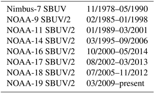
The comparison between lidar and SBUV station overpasses on common days throughout the record was based on deseasonalized monthly mean lidar and SBUV ozone profiles. Figure 1a shows the resulting correlation coefficients which were found to be all statistically significant at the 99.99 % confidence level. Concerning the correlations between lidar data and SBUV overpasses, we calculated monthly averages when at least three common days were available. The data were deseasonalized by subtracting the long-term monthly mean pertaining to the same calendar month. All correlation coefficients (r) were calculated using the Pearson product–moment correlation and were tested for significance using the t test formula for the correlation coefficient with n−2 degrees of freedom (von Storch and Zwiers, 1999):
Recalculation after removing the strong trends before 1998 does not alter the significance. We have confined our analysis to the SBUV layers from 8 (40–25 hPa) up to 14 (2.5–1.6 hPa). This was imposed by the fact that at the highest altitudes lidar data quality is reduced, while at the lowest altitudes SBUV data quality is also reduced. The average distance between the subsatellite point and a lidar station was 500 km at middle latitude stations (Hohenpeißenberg, Haute Provence and Lauder) and 700 km for lower latitude lidar stations (Table Mountain and Mauna Loa) with collocation time criterion being sub daily.
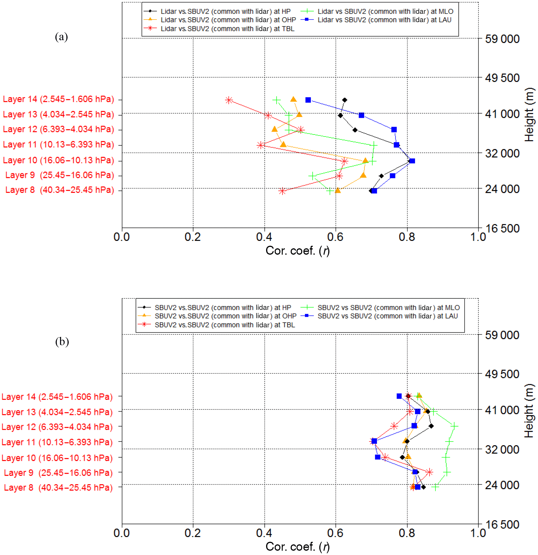
Figure 1(a) Correlation between monthly mean ozone anomalies from lidar and SBUV station overpasses on common days. Best correlations are between 25 and 32 km. All correlations are statistically significant at 99.99 %. HP: Hohenpeißenberg, OHP: Haute Provence, TBL: Table Mountain, MLO: Mauna Loa, LAU: Lauder. (b) Same as in (a) but comparing monthly mean SBUV overpasses from about 30 days in a month with monthly mean SBUV overpasses from only days when lidar measurements were available. All correlations are statistically significant at 99.99 %.
The correlation coefficients in Fig. 1a show a structure in the vertical. This is a result of using different instruments and different sampling times (SBUV data are daytime drifting orbit, lidar data are night-time). The declining signal-to-noise ratio for the lidars above 35 to 40 km also plays a role. Larger atmospheric variability at higher latitudes tends to increase correlations, e.g. at Lauder and Hohenpeißenberg, as does the very regular and large Quasi Biennial Oscillation (QBO) signal at Mauna Loa. To check the effect of different sampling, we also calculated the correlation between monthly mean SBUV overpasses averaged over all ≈ 30 days in a month, with SBUV overpasses averaged only over those days when lidar measurements were available. These results are presented in Fig. 1b. Now the vertical structure is reduced, indicating that the drop above 35 km in Fig. 1a is due to instrumental differences between SBUV and the lidars. The drop in correlation around 32 km in Fig. 1b indicates atmospheric variability that is sampled differently, when measurements are available only on the lidar dates. Interestingly, this variability seems to occur predominantly at the mid-latitude stations, not at Mauna Loa.
We now come to the question of the representativeness of ozone monthly means at single stations compared to 5∘ latitude zonal means calculated for SBUV. Figure 2a shows the profiles of correlations between SBUV monthly 5∘ zonal means and SBUV monthly mean overpasses at the lidar locations. Again, all correlation coefficients are large (0.70 to 0.95) and highly significant (99.99 %). The increase in the correlations with altitude is in part due to the larger trends at higher latitudes, which increase the signal-to-noise ratio on longer timescales. Finally, Fig. 2b gives the correlation between SBUV monthly zonal means and lidar station monthly means. These correlation coefficients are substantially reduced, but are still statistically significant, except at Table Mountain above 10 hPa. The previous figures help to explain the observed range of correlations in Fig. 2b: as shown in Fig. 2a for SBUV data, the correlation between station monthly means and zonal means ranges between 0.8 and 0.9 from a perfect value of 1. This is largely due to longitudinal variations, which are smallest at lower latitudes, e.g. Mauna Loa. Figure 1b, again on the basis of SBUV data, then indicates that the sparse temporal sampling of the lidars leads to correlations between 0.7 to 0.9, compared to the perfect correlation value of 1. Again, this is less critical at Mauna Loa, where either better sampling or lower temporal variability (or both) gives the highest correlations. Figure 1a indicates that instrumental differences between the lidars and SBUV (different vertical resolution, different accuracy, different long-term stability) result in correlations between 0.4 and 0.8 for monthly mean data with comparable sampling. Reduced temporal sampling by the lidars (compare Fig. 1b), and longitudinal variations not sampled by a single station (compare Fig. 2a), together explain the reduced correlations (0.2 to 0.6) between lidar monthly means and SBUV zonal means in Fig. 2b.
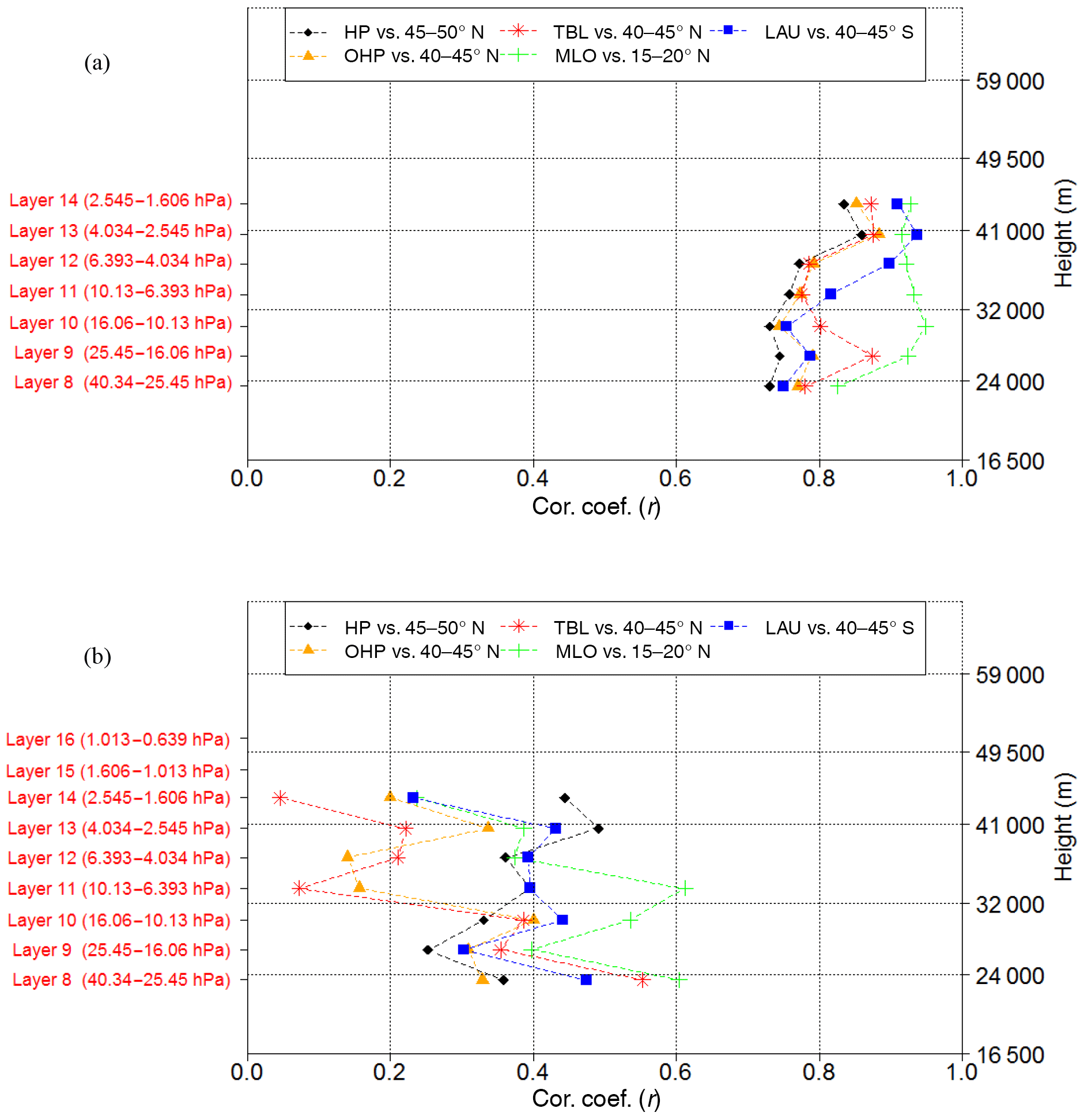
Figure 2(a) Correlations between monthly mean SBUV station overpasses and the corresponding SBUV monthly 5∘ zonal means. (b) Correlations between monthly mean lidar observations and the corresponding SBUV monthly 5∘ zonal means.
A further look at the spatial distribution of correlation coefficients between single SBUV overpasses at lidar stations (or station groups) and SBUV 5∘ zonal means is given in Fig. 3. The correlation coefficients have been calculated using deseasonalized and detrended ozone data. Data were detrended by removing a 2∘ polynomial fit from the deseasonalized time series. The results show that ozone at the five selected lidar stations correlate well with ozone over a fairly wide range of latitudes within ±15∘ centred at the station. This result has little dependence on height. The correlation coefficients found were high and in all cases their statistical significance exceeded 99.99 % (correlations ranging between 0.45 and 0.9 with the highest values near the latitude circle corresponding to each station). The fairly good “zonal representativeness” of the stations is obvious from the colour scale. Here we remind the reader that long-term trends have been removed from the time series and therefore long-term trends do not contribute to the observed correlations.
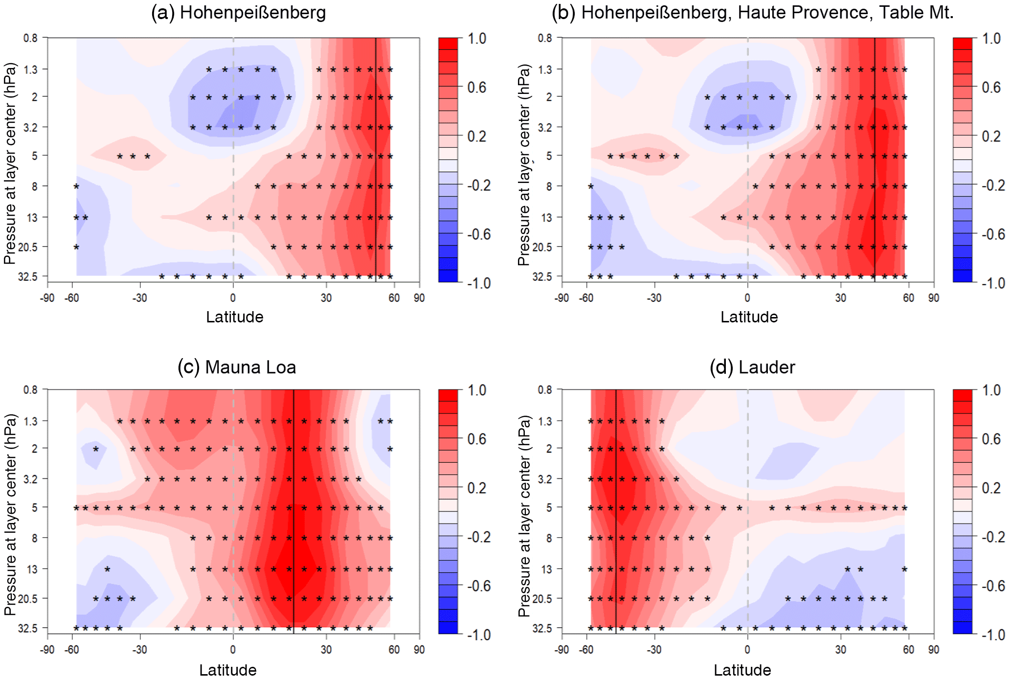
Figure 3(a) Cross section of correlation coefficients between monthly mean SBUV overpasses at Hohenpeißenberg and 5∘ zonal monthly mean SBUV data. (b) Same as (a) but for three combined northern mid-latitude stations (Hohenpeißenberg, Haute Provence and Table Mountain). (c) Same as (a) but for Mauna Loa. (d) Same as (a) but for Lauder. Data have been deseasonalized and detrended (see text). Stippling indicates significance at 95 %. Black vertical lines indicate the latitudes of stations presented in each panel.
A number of proxies have been used to explain the variability in space and time of the vertical ozone distribution, superimposed to the dominating annual cycle (Zerefos et al., 1992; Reinsel et al., 2002; Newchurch et al., 2003; Reinsel et al., 2005; Zanis et al., 2006; Nair et al., 2013; Frith et al., 2014; Harris et al., 2015; Steinbrecht et al., 2017; Weber et al., 2018; WMO Scientific Assessment of Ozone Depletion, 2007, 2011, 2014). Each proxy reflects ozone variability in a different way. For instance, the ENSO has specific geographic patterns of influence in total ozone and its effect is confined in the upper troposphere and/or lower stratosphere (Zerefos et al., 1992). The QBO is influencing ozone from the middle stratosphere down to the troposphere with a phase progressing both in height and latitude at rates of about 1 km per month vertically, and by about 4∘ of latitude per month horizontally (Zerefos, 1983).
The proxies can be grouped into the following categories: (1) Dynamical proxies. These include the Quasi Biennial Oscillation (QBO), the El Niño Southern Oscillation (ENSO), the Arctic Oscillation (AO), the Antarctic Oscillation (AAO) and tropopause pressure. (2) Extraterrestrial proxies. This is primarily the 11-year solar cycle and (3) stratospheric composition proxies, typically stratospheric aerosol optical depth (AOD, e.g. at 525 nm) and equivalent effective stratospheric chlorine (EESC). In order to investigate both qualitatively and quantitatively the attribution of ozone variations to the different proxies, we have used the MLR method, as described in the following section.
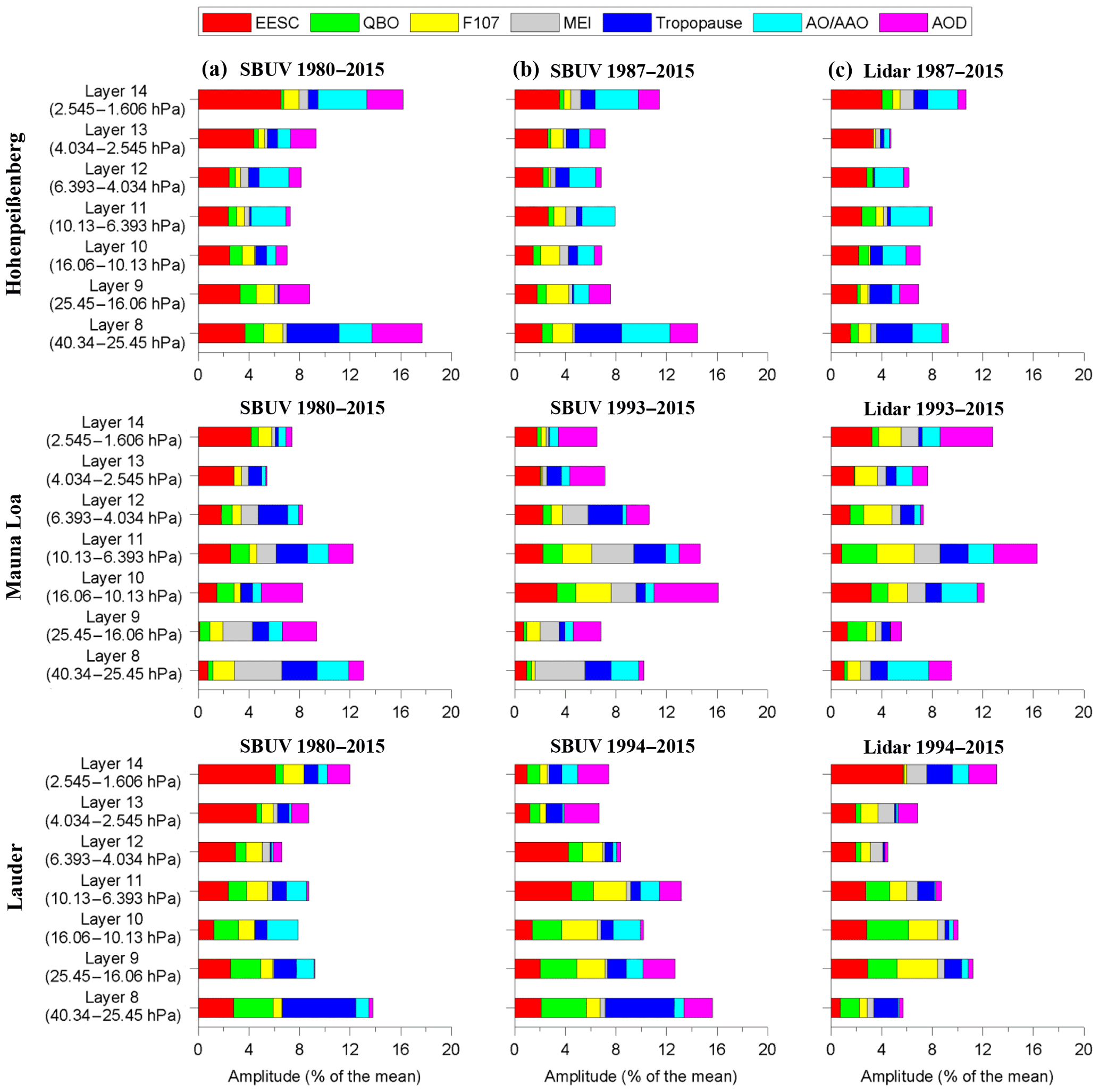
Figure 4Amplitudes, i.e. (max−min)∕2, of ozone variations attributed to EESC and its orthogonal function, QBO, F10.7, MEI, tropopause pressure, AO (or AAO at Lauder) and AOD for each stratospheric layer. All values are expressed in percent of the long-term mean at each layer. Stations shown are: Hohenpeißenberg (47.8∘ N, 11.0∘ E), Mauna Loa (19.5∘ N, 155.6∘ W) and Lauder (45.0∘ S, 169.7∘ E). (a) SBUV overpass data for the full period 1980–2015. (b) SBUV overpass data for common period with lidar, starting in 1987 at Hohenpeißenberg, 1993 at Mauna Loa and 1994 in Lauder. (c) lidar monthly means.
4.1 Regression analysis model
Multivariate linear regression (MLR) analysis has been applied both to SBUV and lidar datasets (e.g. WMO Scientific Assessment of Ozone Depletion, 2011; Nair et al., 2013; Harris et al., 2015). Historically, long-term trends in ozone have been investigated with the use of simple linear trends. More sophisticated methods allowing for the estimation of a change in the long-term trend (such as the piecewise linear trend, PWLT), or directly using the EESC as a proxy to estimate the rate of change in ozone losses due to the evolution of ozone depleting substances (ODSs), have been used, e.g. by Reinsel et al. (2005), Newman et al. (2007) or in the ozone assessments (WMO Scientific Assessment of Ozone Depletion, 2014).
In this work we have used the statistical model in two ways, using either (a) the PWLT method, with January 1998 selected as inflection point, or (b) EESC and its orthogonal function as proxies (Damadeo et al., 2014; Kuttippurath et al., 2015). The MLR regression model, in each case, was applied at all seven pressure levels and for the different zonal belts or stations. Our MLR model takes the following general form:
where the term atrendTrend corresponds to either (a) a PWLT or (b) the EESC proxy:
(a) , in the case of the PWLT runs, with T1 and T2 accounting for pre- and post-1998 linear trends and T2 set to zero before January 1998, and (b) αeescEESC(t), for the runs with EESC and its orthogonal term as proxies.
Overall, ΔO3(t) is the time series of ozone “anomalies” in percent (%) for a particular month t. Data are deseasonalized prior to the analysis by removing the long-term monthly average (1980–2015) for each calendar month (January, February, … December).
The other terms are the following:
-
μ which corresponds to a constant term.
-
For the QBO term, equatorial zonal winds at 30 and 50 hPa as given by the standardized NOAA – CPS indices for 30 and 50 hPa were used (http://www.cpc.ncep.noaa.gov/data/indices/, last access: 2 May 2018).
-
SOLAR accounts for the solar cycle effect in ozone, using the 10.7 cm wavelength solar radio flux (F10.7) as a proxy.
-
Similarly, ENSO accounts for the ENSO effect on ozone, using the MEI (Multivariate ENSO Index) as a proxy http://www.esrl.noaa.gov/psd/enso/mei/table.html (last access: 2 May 2018).
-
The AOI term is used to describe the Arctic (or Antarctic) Oscillation effect on ozone. The AO index is used for the Northern Hemisphere and the AAO index for the Southern Hemisphere. Both come from NOAA: http://www.cpc.ncep.noaa.gov/products/precip/CWlink/daily_ao_index/teleconnections.shtml (last access: 2 May 2018).
-
troppres is the term used to describe the effect of tropopause changes on ozone. This index is constructed from NCEP reanalysis tropopause pressures. It is filtered to remove ENSO, solar, QBO, long-term trend and volcanic effects through MLR analysis. The index is calculated separately for every dataset used here, either as a zonal mean for the SBUV zonal averages or for each station (lidar or SBUV overpasses).
-
AOD is used to describe volcanic effects: the zonal mean 525 nm stratospheric aerosol optical depth integrated from the tropopause upwards is used from the Global Space-based Stratospheric Aerosol Climatology (GloSSAC) dataset (Thomason et al., 2018; https://doi.org/10.5067/GloSSAC-L3-V1.0).
-
N(t) is the residual noise series, assumed to be an autoregressive AR(1) time series with , where ε(t) is an uncorrelated series, with weights inversely proportional to the monthly residual variances, in which the uncertainties in the monthly averages were taken into account.
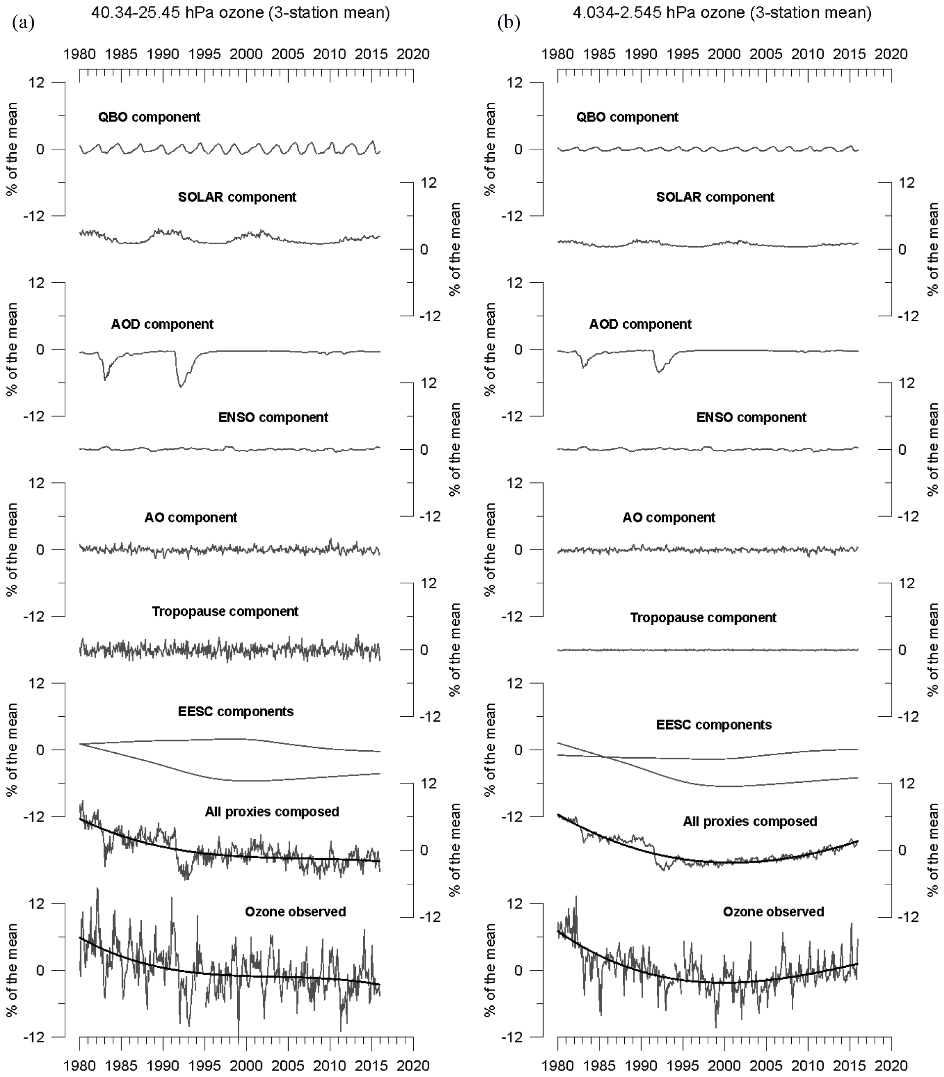
Figure 5(a) Ozone variations attributed to the different proxies (QBO, SOLAR, AOD, ENSO, AO, tropopause pressure, EESC and its orthogonal function) at layer 8 (40.34–25.45 hPa, centred at about 24 km height) for SBUV overpasses averaged over Hohenpeißenberg, Haute Provence and Table Mountain. (b) Same as in (a) but for layer 13 (4.034–2.545 hPa) centred at about 40 km height. The lower most curves give the observed deseasonalized SBUV time series. Thick solid curves in the four bottom panels are third degree polynomials fit to the data.

Figure 6Ozone anomalies from SBUV overpasses averaged over Hohenpeißenberg, Haute Provence and Table Mountain. Top: original deseasonalized time series. Middle: time series with natural proxies removed, but EESC-related variations remaining. Bottom: time series with natural proxies and orthogonal EESC-related variations removed. (a) For layer 8 (40.34–25.45 hPa, centred at about 24 km height). (b) Same as in (a) but for the layer 13 (4.034–2.545 hPa) centred at about 40 km height. MK test refers to the Mann–Kendall trend test. Thick solid curves are third degree polynomials fit to the data.
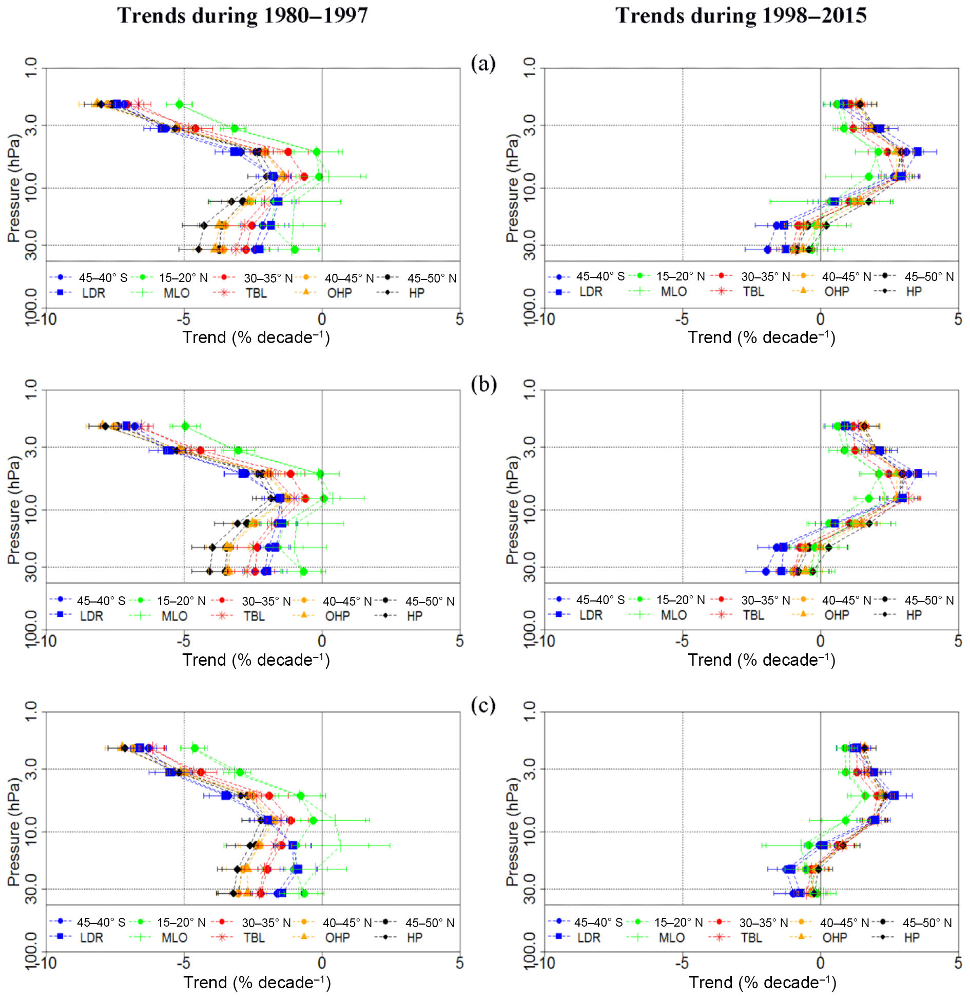
Figure 7Trends in the vertical distribution of ozone for the pre-1998 and post-1998 period, based on SBUV station overpass and zonal mean data, using (a) two linear trend terms and volcanic effects only, (b) the PWLT method including all proxies and (c) using all proxies and two orthogonal EESC terms to describe the long-term ozone changes. The results are based on SBUV overpasses and SBUV zonal means.
Trends and errors (especially for the PLWT runs) are calculated as in Reinsel et al. (2002) and the results are given in percent of the respective long-term mean.
4.2 MLR results and discussion
Figure 4 shows the amplitude (maximum value minus minimum value all divided by two) of ozone variability attributed to each proxy for the seven vertical layers and for Hohenpeißenberg, Mauna Loa and Lauder. Amplitudes are given in percent of the long-term ozone mean. The upper panels of Fig. 4 show results for Hohenpeißenberg as a northern mid-latitude example, the middle panels for Mauna Loa as a tropical latitude and the bottom panels for Lauder as a southern mid-latitude example. The left plots refer to monthly mean SBUV overpasses for the whole period 1980–2015, the middle plots refer to SBUV data for the period common with lidar measurements and the right plots refer to the lidar monthly mean ozone profiles. The amplitude of QBO-related variations below 10 hPa, down to 40 hPa, is on the order of 2 % of the mean. The smallest QBO amplitudes are found in the uppermost layers 13 and 14 (0.5 % of the mean or less). We should point out that according to Kramarova et al. (2013) the coarse vertical resolution of SBUV (and the decreasing altitude resolution of the lidars above 35 to 40 km) can induce errors in the amplitude of QBO-related ozone anomalies on the order of 1 % at heights between 10 and 1 hPa. However, for trend analysis purposes this is not expected to have any significant effect.
The footprint of the solar cycle is clearly seen in the middle and upper stratosphere with amplitudes around 2 % of the mean. The amplitude of AO (AAO in the Southern Hemisphere) in the zonal mean is about 1 % of the mean. At individual levels or stations it can be as high as 4 % of the mean. The contribution of ENSO (MEI) is typically less than 1 % of the mean at Hohenpeißenberg and Lauder, but up to 4 % for the Mauna Loa SBUV data.
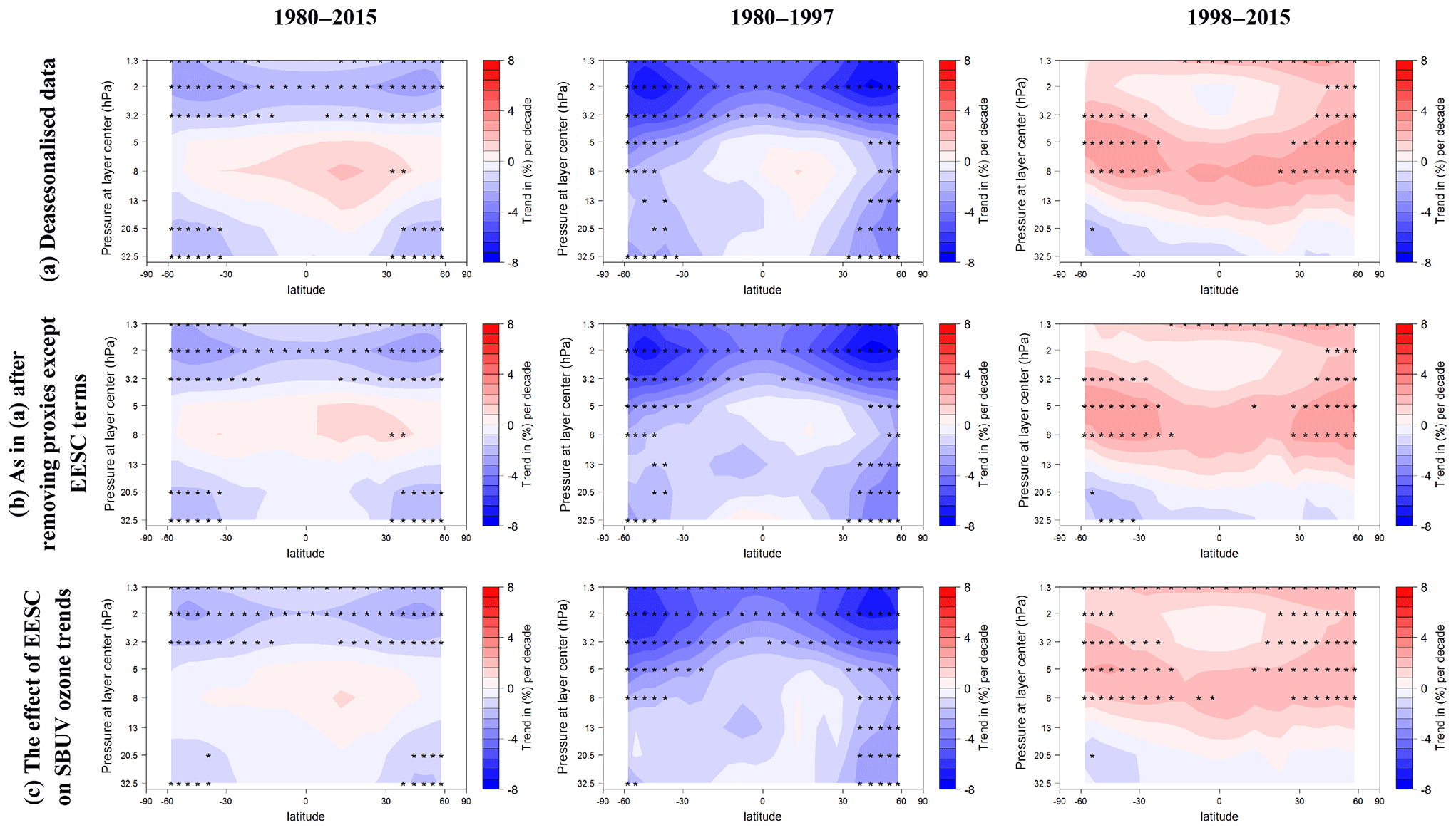
Figure 8Cross section of ozone trends from zonal mean SBUV (1980–2015, left), (1980–1997, middle) and (1998-2015, right) in percent per decade. Rows as in Fig. 7, (a) PWLT, no proxies except AOD, (b) PWLT with all proxies, bottom: trends from two fitted orthogonal EESC terms. Stippling indicates significance at 95 %. Data are averaged over 5∘ of latitude zones.
The effect of tropopause height variations is most evident in the lower stratospheric layer 8, where it reaches 4 % for the SBUV data at Lauder and Hohenpeißenberg, but only 2 % for the lidar data. The lidars have better altitude resolution than SBUV in the lower- and mid-stratosphere, and do not include a substantial contribution from levels below 40 hPa or 26 km. In the upper levels, tropopause-height-related ozone variations generally decrease. Transient effects from large AOD of volcanic origin (El Chichon, Mount Pinatubo) can contribute substantially to the ozone variability, from 4 to 6 % of the mean, but for shorter time periods (2 to 3 years) after the volcano. Finally, the EESC proxies representing halogen chemistry carry the largest and most significant ozone variations, up to 5 % of the mean in the upper stratosphere. These results are in general agreement with previous results by Nair et al. (2013) and Kirgis et al. (2013).
As it appears from Fig. 4, the percent of the total variability explained by all proxies taken together ranges between 5 and 15 % of the mean, both for the lidar and the SBUV overpasses. Additionally there appears to be poorer agreement for Lauder than for the other stations. It should be noted here that both Lauder and Mauna Loa lidar records start 1–2 years after the Mount Pinatubo eruption and this makes it difficult to separate the influence of volcanic aerosol from other proxies at these two stations, but not at Hohenpeissenberg because of its longer record.
The temporal evolution of ozone variations attributed to natural proxies and to EESC terms is presented in Fig. 5. That figure shows time series of ozone anomalies and regression results from 1980 to 2015 SBUV monthly mean overpasses, averaged over three stations (Hohenpeißenberg, Haute Provence and Table Mountain). Two stratospheric layers are shown: layer 8 (40.34–25.45 hPa) centred at about 24 km height and layer 13 (4.034–2.545 hPa) centred at about 40 km height. Figure 5 shows that the major long-term variations come from the two orthogonal EESC terms, the solar cycle and AOD. The major contribution from AOD is highly limited to the two periods with the strong volcanic eruptions (El Chichon and Mount Pinatubo). Interesting to note here is the fact that in some particular years the synergistic contribution of shorter-term variations can result in substantial additive anomalies. This might or might not influence the estimation of long-term changes or trends in the ozone profile. Notable synergistic negative anomalies can be seen in the years 1983, 1985, 1988, 1992, 1993, 1995, 1997, 1999, 2002, 2004, 2006, 2008, 2011 and 2013 in which the negative phase of QBO and of other proxies coincided. Further analysis, however, showed that, even after removing the above years, the observed trends remained the same. Therefore we conclude that the synergistic effect by different proxies has not influenced the trend estimates discussed before. Finally we note here that the correlations between the regressed time series (all proxies composed) and the observed ozone anomalies are 0.62 for layer 8 (t value = 16.19, p value < 0.0001, N= 426) and 0.67 for layer 13 (t value = 18.59, p value < 0.0001, N= 426).
Another look at the long-term ozone variations is given in Fig. 6. The upper time series in the figure shows the observed SBUV overpass anomalies, the middle series the variations explained by natural influences (i.e. all proxies except the orthogonal EESC terms) and the lower series shows the remaining ozone residuals after all natural influences and the orthogonal EESC terms (all proxies) have been removed, for the whole 36-year period (1980–2015) and for layers 8 (left) and 13 (right). From Fig. 6a and b one can clearly see that removing the natural proxies has little effect on the slowly moving long-term ozone trends. Most of the long-term variability is congruent with the EESC proxies, especially in the upper stratospheric layer 13. The same figure shows that in the lower stratosphere a small negative tendency prevails after the end of the 1990s and a small positive tendency is seen in the upper stratosphere. After removing the variability attributed to all proxies (natural and orthogonal EESC terms), the nonparametric Mann–Kendall rank statistic trend test (Mitchell et al., 1966) was applied to the anomaly series. It was found that both in the upper and lower stratosphere the overall trends (1980–2015) were insignificant at the 99 % confidence level.
Various authors (Newchurch, 2003; Reinsel et al., 2005; Zanis et al., 2006; Zerefos et al., 2012; Harris et al., 2015; Solomon et al., 2016; Steinbrecht et al., 2017) provide evidence for a difference in ozone “trends” before and after the years 1996 and 1998. Using the MLR model described in Sect. 4.1 we have calculated linear trends, with and without including the various proxies listed in Sect. 4.1, for the SBUV zonal means and SBUV overpasses over the lidar stations. Trends were calculated using the PWLT method (January 1998 set as the inflection point). In a separate run we used EESC and its orthogonal function to describe the ozone trends, and from that calculated the EESC orthogonal-related ozone trends before and after 1998.
As a first step, we performed a base-line run, fitting only the two linear trend terms (denoted as T1 and T2 in Sect. 4.1) and the volcanic effect (AOD). This gives the pre- and post-1998 trends in Fig. 7a. Then a run with the PWLT method was performed accounting for the effects of QBO, ENSO, solar cycle, tropopause variability, AO, AAO and volcanic effects, and including the two linear trend terms T1 and T2 for the same inflection point. The resulting trends are displayed in Fig. 7b (mid-row). Finally, we performed a run with all proxies, but using EESC and its orthogonal term instead of PWLT. The corresponding ozone trends before and after 1998, due to the fitted orthogonal EESC terms, are presented in Fig. 7c (bottom row).
Comparison of the trends presented in Fig. 7a and b, both calculated using linear trend terms (PWLT), shows minor changes only. Clearly this signifies that different proxies have very little effect on the trends. The proxy that has the largest influence on trends is the solar cycle, a result based on 36 years of data. Comparison between Fig. 7b and c shows that for the pre-1998 period (left panels) trends are very similar (almost identical), regardless if a linear trend term (the pre-1998 part of the PWLT method) or the orthogonal EESC terms are used. For the post-1998 period (right panels), the resulting trends do not change significantly when comparing Fig. 7a, b and c.
While trends calculated with the use of EESC reflect the effect of changes in ODS on ozone, PWLT linear trends can interact to other long-term changes, e.g. to effects of increasing green house gases (GHGs) and global warming (e.g. Jonsson et al., 2004; Zerefos et al., 2014). Chemistry-climate model simulations assessing the effects of changes in ODS and/or GHGs indicate that their contributions add linearly to produce the overall ozone change (see detailed discussion and references in WMO Scientific Assessment of Ozone Depletion, 2014; Sect. 2.3.5.2). We note here that the comparison of Fig. 7b and c reduces the importance of the GHG effect on the observed small differences between b and c; always remember that our study is confined to the region between 30 and 2 hPa.
Although the period (1998–2015) is slightly larger from the period studied by Frith et al. (2017) (2001–2015) the results reported here are in general agreement with the SBUV trends reported in that study. Finally, it should be noted that the profiles of trends from SBUV station overpasses (dashed lines) and trends for the 5∘ latitudinal belts (solid lines) are very similar for both periods of study (1980–1997 and 1998–2015).
Figure 8 extends the previous findings to a global perspective, based on SBUV zonal means. All cross sections in Fig. 8 are plotted against the sine of latitude north and south in order that tropical areas are represented in their proper dimension. The tick marks of the vertical axis are centred at the indicated pressure level. The colour scale gives the calculated trends in percent per decade. The first vertical group of cross sections refers to the period 1980–2015, the middle to the period 1980–1997 and the right to the period 1998–2015. Comparing the observed trends during the different periods, we see that there is a region between 10 and 5 hPa over the tropics which shows positive ozone trends over the whole 1980 to 2015 period of record, and to a different degree also in the two sub-periods. These trends, however, are not statistically significant. Also notable are the negative trends over middle and high latitudes below 15 hPa, both in the total 1980 to 2015 period and in both sub-periods. The big change when dividing the 1980–2015 period into two sub-periods is the change in sign of the observed trends in the upper stratosphere, as well as in parts of the middle stratosphere, particularly over middle and high latitudes (upper set of cross sections). Trends in the lower stratosphere continue to be negative as reported by Ball et al. (2018).
The middle and lower sets of cross sections in Fig. 8 are plotted to provide preliminary answers to the effect of including natural proxies, and to the agreement between PWLT and trends using the prescribed EESC and its orthogonal function curves. It is obvious from the top and middle panels of Fig. 8 that adding or removing the natural proxies has little effect on the observed trends. At any rate a separate analysis (not shown here) confirms that adding or removing of AOD has little and an insignificant effect on the trends. The general similarity between the middle and bottom set of cross sections in Fig. 8 points out the importance of anthropogenic ODSs, represented by EESC and its orthogonal function, from the middle to the upper stratosphere.
This paper investigates the representativeness of single lidar stations to calculate trends in the vertical ozone profiles. From 40 hPa to the upper stratosphere, single or grouped stations correlate well with zonal means calculated from SBUV overpasses. A good correlation (> 0.4) with zonal means is found within ±15∘ of latitude north or south of any lidar station with little dependence on height. This is because at the highest altitudes lidar data quality is reduced, while at the lowest altitudes SBUV data quality are reduced; we have confined our analysis to the SBUV layers from 8 (40–25 hPa) to 14 (2.5–1.6 hPa). Ozone trend profiles are very similar over the different stations and their corresponding zonal means. A detailed analysis of proxy footprints in the vertical ozone profiles also shows large similarities between lidar time series at the stations, the SBUV overpass time series and the SBUV zonal means.
Ozone trends have been studied with and without the inclusion of additional proxies, and for the full period 1980–2015, as well as for the two sub-periods 1980–1997 and 1998–2015. The major contribution to the trends comes from anthropogenic ODSs (EESC) and its orthogonal function, and to a much lesser extent to the solar cycle and AOD. Long-term trends were not influenced by adding all other proxies, although these can produce significant negative anomalies in certain years; for example in 1983, 1985, 1988, 1992, 1993, 1995, 1997, 1999, 2002, 2004, 2006, 2008, 2011 and 2013.
The so-called “inflection point” between 1997 and 1999 marks the change from previously significant negative ozone trends to recent positive ozone trends (1998–2015) mostly at levels above 15 hPa. Ozone trends in the two sub-periods before and after 1998 have been further compared with a multiple regression model with piece-wise linear trends (PWLT), with and without natural proxies, or with EESC and its orthogonal function representing the effects of anthropogenic ODSs. Natural proxies had little effect on the observed trends in both periods before and after 1998. The largest contributor to the observed ozone trends in both periods were the anthropogenic ODS. At lower heights between 15 and 40 hPa, the pre-1998 negative ozone trends tend to become less significant as we move towards 2015, below which recent literature reports the continuation of the lower stratosphere ozone decline.
Satellite ozone data from the Solar Backscatter Ultraviolet Radiometer (SBUV) overpassing Hohenpeißenberg, Haute Provence, Table Mountain, Mauna Loa and Lauder were obtained from ftp://toms.gsfc.nasa.gov/pub/sbuv/AGGREGATED/ (last access: 2 May 2018) (McPeters et al., 2012; Bhartia et al., 2013). Additional SBUV data at 5∘ of latitude zonal means were taken from ftp://toms.gsfc.nasa.gov/pub/MergedOzoneData/Ind_Inst_HDF/ (last access: 2 May 2018; McPeters et al., 2012; Bhartia et al., 2013). Ground-based lidar ozone profiles were obtained from the Network for the Detection of Atmospheric Composition Change (NDACC) database at ftp://ftp.cpc.ncep.noaa.gov/ndacc/station/ (last access: 2 May 2018; De Mazière et al., 2018).
The authors declare that they have no conflict of interest.
Quadrennial Ozone Symposium 2016 – Status and trends of atmospheric ozone (ACP/AMT inter-journal SI) SI statement: this article is part of the special issue “Quadrennial Ozone Symposium 2016 – Status and trends of atmospheric ozone (ACP/AMT inter-journal SI)”. It is a result of the Quadrennial Ozone Symposium 2016, Edinburgh, United Kingdom, 4–9 September 2016.
The authors acknowledge the Mariolopoulos-Kanaginis Foundation for the
Environmental Sciences for funding this research, the Copernicus Atmosphere
Monitoring Service (CAMS-84) and the project of EUMETSAT AC SAF.
We acknowledge the NDACC network and the individual agencies and scientists responsible for
the ground-based lidar ozone measurements, particularly Thierry Leblanc for
the Mauna Loa and Table Mountain lidars, and Daan Swart and Ann van Gijsel
for the Lauder lidar, as well as the SBUV science team for providing the
satellite ozone profiles. Birgit Hassler would like to thank DLR-IPA in
Oberpfaffenhofen, Germany for funding a three-month stay as visiting
scientist that allowed her to work on this study. The authors would like to
thank the two anonymous reviewers for their constructive comments and
suggestions.
Edited by: Mark
Weber
Reviewed by: two anonymous referees
Ball, W. T., Alsing, J., Mortlock, D. J., Staehelin, J., Haigh, J. D., Peter, T., Tummon, F., Stübi, R., Stenke, A., Anderson, J., Bourassa, A., Davis, S. M., Degenstein, D., Frith, S., Froidevaux, L., Roth, C., Sofieva, V., Wang, R., Wild, J., Yu, P., Ziemke, J. R., and Rozanov, E. V.: Evidence for a continuous decline in lower stratospheric ozone offsetting ozone layer recovery, Atmos. Chem. Phys., 18, 1379–1394, https://doi.org/10.5194/acp-18-1379-2018, 2018.
Bhartia, P. K., McPeters, R. D., Flynn, L. E., Taylor, S., Kramarova, N. A., Frith, S., Fisher, B., and DeLand, M.: Solar Backscatter UV (SBUV) total ozone and profile algorithm, Atmos. Meas. Tech., 6, 2533–2548, https://doi.org/10.5194/amt-6-2533-2013, 2013.
Damadeo, R. P., Zawodny, J. M., and Thomason, L. W.: Reevaluation of stratospheric ozone trends from SAGE II data using a simultaneous temporal and spatial analysis, Atmos. Chem. Phys., 14, 13455–13470, https://doi.org/10.5194/acp-14-13455-2014, 2014.
DeLand, M. T., Taylor, S. L., Huang, L. K., and Fisher, B. L.: Calibration of the SBUV version 8.6 ozone data product, Atmos. Meas. Tech., 5, 2951–2967, https://doi.org/10.5194/amt-5-2951-2012, 2012.
De Mazière, M., Thompson, A. M., Kurylo, M. J., Wild, J. D., Bernhard, G., Blumenstock, T., Braathen, G. O., Hannigan, J. W., Lambert, J.-C., Leblanc, T., McGee, T. J., Nedoluha, G., Petropavlovskikh, I., Seckmeyer, G., Simon, P. C., Steinbrecht, W., and Strahan, S. E.: The Network for the Detection of Atmospheric Composition Change (NDACC): history, status and perspectives, Atmos. Chem. Phys., 18, 4935–4964, https://doi.org/10.5194/acp-18-4935-2018, 2018.
Frith, S. M., Kramarova, N. A., Stolarski, R. S., McPeters, R. D., Bhartia, P. K., and Labow G. J.: Recent changes in total column ozone based on the SBUV Version 8.6 Merged Ozone Data Set, J. Geophys. Res.-Atmos., 119, 9735–9751, https://doi.org/10.1002/2014JD021889, 2014.
Frith, S. M., Stolarski, R. S., Kramarova, N. A., and McPeters, R. D.: Estimating uncertainties in the SBUV Version 8.6 merged profile ozone data set, Atmos. Chem. Phys., 17, 14695–14707, https://doi.org/10.5194/acp-17-14695-2017, 2017.
Harris, N. R. P., Hassler, B., Tummon, F., Bodeker, G. E., Hubert, D., Petropavlovskikh, I., Steinbrecht, W., Anderson, J., Bhartia, P. K., Boone, C. D., Bourassa, A., Davis, S. M., Degenstein, D., Delcloo, A., Frith, S. M., Froidevaux, L., Godin-Beekmann, S., Jones, N., Kurylo, M. J., Kyrölä, E., Laine, M., Leblanc, S. T., Lambert, J.-C., Liley, B., Mahieu, E., Maycock, A., de Mazière, M., Parrish, A., Querel, R., Rosenlof, K. H., Roth, C., Sioris, C., Staehelin, J., Stolarski, R. S., Stübi, R., Tamminen, J., Vigouroux, C., Walker, K. A., Wang, H. J., Wild, J., and Zawodny, J. M.: Past changes in the vertical distribution of ozone – Part 3: Analysis and interpretation of trends, Atmos. Chem. Phys., 15, 9965–9982, https://doi.org/10.5194/acp-15-9965-2015, 2015.
Jonsson, A. I., de Grandpré, J., Fomichev, V. I., McConnell, J. C., and Beagley, S. R.: Doubled CO2-induced cooling in the middle atmosphere: photochemical analysis of the ozone radiative feedback, J. Geophys. Res., 109, D24103, https://doi.org/10.1029/2004JD005093, 2004.
Kirgis, G., Leblanc, T., McDermid, I. S., and Walsh, T. D.: Stratospheric ozone interannual variability (1995–2011) as observed by lidar and satellite at Mauna Loa Observatory, HI and Table Mountain Facility, CA, Atmos. Chem. Phys., 13, 5033–5047, https://doi.org/10.5194/acp-13-5033-2013, 2013.
Kramarova, N. A., Bhartia, P. K., Frith, S. M., McPeters, R. D., and Stolarski, R. S.: Interpreting SBUV smoothing errors: an example using the quasi-biennial oscillation, Atmos. Meas. Tech., 6, 2089–2099, https://doi.org/10.5194/amt-6-2089-2013, 2013.
Kuttippurath, J., Bodeker, G. E., Roscoe, H. K., and Nair, P. J.: A cautionary note on the use of EESC-based regression analysis for ozone trend studies, Geophys. Res. Lett., 42, 162–168, https://doi.org/10.1002/2014GL062142, 2015.
McPeters, R. D., Bhartia, P. K., Haffner, D., Labow, G. J., and Flynn, L.: The version 8.6 SBUV ozone data record: An overview, J. Geophys. Res.-Atmos., 118, 8032–8039, https://doi.org/10.1002/jgrd.50597, 2013.
Mitchell, J. M., Dzerdzeevskii, B., Flohn, H., Hofmeyr, W. L., Lamb, H. H., Rao, K. N., and Wallén, C. C.: Climatic change: report of a working group of the Commission for Climatology, Technical Note No. 79, WMO-No. 195. TP. 100, World Meteorological Organization, Geneva, Switzerland, available at: https://library.wmo.int/opac/index.php?lvl=notice_display&id=3849#.WilBr0pl-Uk (last access: 2 May 2018), 1966.
Nair, P. J., Godin-Beekmann, S., Kuttippurath, J., Ancellet, G., Goutail, F., Pazmiño, A., Froidevaux, L., Zawodny, J. M., Evans, R. D., Wang, H. J., Anderson, J., and Pastel, M.: Ozone trends derived from the total column and vertical profiles at a northern mid-latitude station, Atmos. Chem. Phys., 13, 10373–10384, https://doi.org/10.5194/acp-13-10373-2013, 2013.
Newchurch, M. J., Yang, E.-S., Cunnold, D. M., Reinsel, G. C., Zawodny, J. M., and Russell, J. M.: Evidence for slowdown in stratospheric ozone loss: first stage of ozone recovery, J. Geophys. Res., 108, 4507, https://doi.org/10.1029/2003JD003471, 2003.
Newman, P. A., Daniel, J. S., Waugh, D. W., and Nash, E. R.: A new formulation of equivalent effective stratospheric chlorine (EESC), Atmos. Chem. Phys., 7, 4537–4552, https://doi.org/10.5194/acp-7-4537-2007, 2007.
Reinsel, G. C., Weatherhead, E. C., Tiao, G. C., Miller, A. J., Nagatani, R. M., Wuebbles, D. J., and Flynn, L. E.: On detection of turnaround and recovery in trend for ozone, J. Geophys. Res., 107, 4078, https://doi.org/10.1029/2001JD000500, 2002.
Reinsel, G. C., Miller, A. J., Weatherhead, E. C., Flynn, L. E., Nagatani, R. M., Tiao, G. C., and Wuebbles, D. J.: Trend analysis of total ozone data for turnaround and dynamical contributions, J. Geophys. Res., 110, D16306, https://doi.org/10.1029/2004JD004662, 2005.
Solomon, S., Ivy, D. J., Kinnison, D., Mills, M. J., Neely III, R. R., and Schmidt, A.: Emergence of healing in the Antarctic ozone layer, Science, 353, 269–274, https://doi.org/10.1126/science.aae0061, 2016.
Steinbrecht, W., Froidevaux, L., Fuller, R., Wang, R., Anderson, J., Roth, C., Bourassa, A., Degenstein, D., Damadeo, R., Zawodny, J., Frith, S., McPeters, R., Bhartia, P., Wild, J., Long, C., Davis, S., Rosenlof, K., Sofieva, V., Walker, K., Rahpoe, N., Rozanov, A., Weber, M., Laeng, A., von Clarmann, T., Stiller, G., Kramarova, N., Godin-Beekmann, S., Leblanc, T., Querel, R., Swart, D., Boyd, I., Hocke, K., Kämpfer, N., Maillard Barras, E., Moreira, L., Nedoluha, G., Vigouroux, C., Blumenstock, T., Schneider, M., García, O., Jones, N., Mahieu, E., Smale, D., Kotkamp, M., Robinson, J., Petropavlovskikh, I., Harris, N., Hassler, B., Hubert, D., and Tummon, F.: An update on ozone profile trends for the period 2000 to 2016, Atmos. Chem. Phys., 17, 10675–10690, https://doi.org/10.5194/acp-17-10675-2017, 2017.
Thomason, L. W., Ernest, N., Millán, L., Rieger, L., Bourassa, A., Vernier, J.-P., Manney, G., Luo, B., Arfeuille, F., and Peter, T.: A global space-based stratospheric aerosol climatology: 1979–2016, Earth Syst. Sci. Data, 10, 469–492, https://doi.org/10.5194/essd-10-469-2018, 2018.
von Storch, H. and Zwiers, F. W.: Statistical analysis in climate research, Cambridge University Press, Cambridge, ISBN 0 521 45071 3, 484 pp., 1999.
Weber, M., Coldewey-Egbers, M., Fioletov, V. E., Frith, S. M., Wild, J. D., Burrows, J. P., Long, C. S., and Loyola, D.: Total ozone trends from 1979 to 2016 derived from five merged observational datasets – the emergence into ozone recovery, Atmos. Chem. Phys., 18, 2097–2117, https://doi.org/10.5194/acp-18-2097-2018, 2018.
WMO Scientific Assessment of Ozone Depletion: 2006, Global Ozone Research and Monitoring Project-Report No. 50, WMO (World Meteorological Organization), Geneva, Switzerland, available at: https://www.esrl.noaa.gov/csd/assessments/ozone/ (last access: 2 May 2018), 2007.
WMO Scientific Assessment of Ozone Depletion: 2010, Global Ozone Research and Monitoring Project-Report No. 52, WMO (World Meteorological Organization), Geneva, Switzerland, available at: https://www.esrl.noaa.gov/csd/assessments/ozone/ (last access: 2 May 2018), 2011.
WMO Scientific Assessment of Ozone Depletion: 2014, Global Ozone Research and Monitoring Project-Report No. 55, WMO (World Meteorological Organization), Geneva, Switzerland, available at: https://www.esrl.noaa.gov/csd/assessments/ozone/ (last access: 2 May 2018), 2014.
Zanis, P., Maillard, E., Staehelin, J., Zerefos, C., Kosmidis, E., Tourpali, K., and Wohltmann, I.: On the turnaround of stratospheric ozone trends deduced from the reevaluated Umkehr record of Arosa, Switzerland, J. Geophys. Res., 111, D22307, https://doi.org/10.1029/2005JD006886, 2006.
Zerefos, C. S.: On the quasi-biennial oscillation in equatorial stratospheric temperatures and total ozone, Adv. Space Res., 2, 177–181, 1983.
Zerefos, C. S., Bais, A. F., Ziomas, I. C., and Bojkov, R. D.: On the relative importance of quasi-biennial oscillation and El Nino/southern oscillation in the revised Dobson total ozone records, J. Geophys. Res., 97, 10135–10144, 1992.
Zerefos, C. S., Tourpali, K., Eleftheratos, K., Kazadzis, S., Meleti, C., Feister, U., Koskela, T., and Heikkilä, A.: Evidence of a possible turning point in solar UV-B over Canada, Europe and Japan, Atmos. Chem. Phys., 12, 2469–2477, https://doi.org/10.5194/acp-12-2469-2012, 2012.
Zerefos, C. S., Tourpali, K., Zanis, P., Eleftheratos, K., Repapis, C., Goodman, A., Wuebbles, D., Isaksen, I. S. A., and Luterbacher, J.: Evidence for an earlier greenhouse cooling effect in the stratosphere before 1980 over the Northern Hemisphere, Atmos. Chem. Phys., 14, 7705–7720, https://doi.org/10.5194/acp-14-7705-2014, 2014.
- Abstract
- Introduction
- Data, analysis and methods
- Representativeness of single station ozone profiles in comparison to zonal means
- The role of proxies in the variability in ozone
- Stratospheric ozone trends before and after 1998
- Conclusions
- Data availability
- Competing interests
- Special issue statement
- Acknowledgements
- References