the Creative Commons Attribution 4.0 License.
the Creative Commons Attribution 4.0 License.
 | 02 May 2018
Decadal evolution of ship emissions in China from 2004 to 2013 by using an integrated AIS-based approach and projection to 2040
Cheng Li
Jens Borken-Kleefeld
Junyu Zheng
Zibing Yuan
Jiamin Ou
Yue Li
Yanlong Wang
Yuanqian Xu
Ship emissions contribute significantly to air pollution and pose health risks to residents of coastal areas in China, but the current research remains incomplete and coarse due to data availability and inaccuracy in estimation methods. In this study, an integrated approach based on the Automatic Identification System (AIS) was developed to address this problem. This approach utilized detailed information from AIS and cargo turnover and the vessel calling number information and is thereby capable of quantifying sectoral contributions by fuel types and emissions from ports, rivers, coastal traffic and over-the-horizon ship traffic. Based upon the established methodology, ship emissions in China from 2004 to 2013 were estimated, and those to 2040 at 5-year intervals under different control scenarios were projected. Results showed that for the area within 200 nautical miles (Nm) of the Chinese coast, SO2, NOx, CO, PM10, PM2.5, hydrocarbon (HC), black carbon (BC) and organic carbon (OC) emissions in 2013 were 1010, 1443, 118, 107, 87, 67, 29 and 21 kt yr−1, respectively, which doubled over these 10 years. Ship sources contributed ∼ 10 % to the total SO2 and NOx emissions in the coastal provinces of China. Emissions from the proposed Domestic Emission Control Areas (DECAs) within 12 Nm constituted approximately 40 % of the all ship emissions along the Chinese coast, and this percentage would double when the DECA boundary is extended to 100 Nm. Ship emissions in ports accounted for about one-quarter of the total emissions within 200 Nm, within which nearly 80 % of the emissions were concentrated in the top 10 busiest ports of China. SO2 emissions could be reduced by 80 % in 2020 under a 0.5 % global sulfur cap policy. In comparison, a similar reduction of NOx emissions would require significant technological change and would likely take several decades. This study provides solid scientific support for ship emissions control policy making in China. It is suggested to investigate and monitor the emissions from the shipping sector in more detail in the future.
- Article
(9381 KB) -
Supplement
(2391 KB) - BibTeX
- EndNote


Although a reduction in ambient PM2.5 levels of more than 30 % has been achieved during the past several years in major city clusters in China due to stringent control measures, the ambient PM2.5 levels are still far higher than the World Health Organization (WHO) Air Quality Guidelines of a 10 g m−3 annual average. Strengthened reduction efforts are needed to reduce the adverse impact of ambient PM2.5 on public health. In comparison with tightened controls on power plants, industry and road vehicle sectors, controls on ship emissions, one of the most significant contributors to ambient PM2.5 pollution along the river and in coastal areas (Liu et al., 2016), are still lax in China. Ship emissions control has been put on the agenda of PM2.5 reduction in the coming years (Ye, 2014; Yang et al., 2015; Fu et al., 2016).
However, estimation of ship emissions in China remain incomplete and largely inaccurate. Locally, ship emission inventories are generally compiled in limited provinces and ports (Fu et al., 2012; Bao et al., 2014; Song, 2014; Tan et al., 2014; Yang et al., 2015), while in global inventories, ship emissions from China are of coarse temporal (monthly) and spatial (1∘ × 1∘) resolutions (Endresen et al., 2003; Corbett et al., 2007; Paxian et al., 2010). A recent study develops ship emission inventory in Asia with spatial resolution of 3 km × 3 km (Liu et al., 2016); however, characteristics of coastal and ship traffic emissions, sector-based contributions in Chinese ports, and their temporal characteristics remain unknown. Furthermore, estimates from domestic (Fan et al., 2016; Li et al., 2016) and international studies (Endresen et al., 2003, 2007; Corbett and Koehler, 2003; Corbett et al., 2007) are associated with large uncertainties due to inconsistency in estimation approaches and data sources, thus hampering the formulation of an effective ship emissions control strategy. Therefore, detailed and reliable ship emission inventories are needed to estimate the potential of ship emission reduction and the formulation of air pollution and public health improvement strategies.
The Automatic Identification System (AIS), an automatic vessel position reporting system, has been widely recognized as a reliable data source that can significantly reduce the uncertainty in ship activities and their geographic distribution (Wang et al., 2008; Dalsøren et al., 2009; Bandemehr et al., 2015). The accuracy of ship emissions estimates based on cargo volumes (Schrooten et al., 2009) and vessel arrived numbers (Yang et al., 2007; Yau et al., 2012; Li et al., 2016) can be improved by using AIS data. Recent studies use AIS data to estimate emissions from all ships at a given time or each single trip in an entire year in Asia and Europe (Liu et al., 2016; Jalkanen et al., 2016). However, the entire AIS database is not freely available to the public, especially in East Asia, and the data before 2012 are not suitable for use due to significant absence of data from a limited number of satellites and shore-based radar sources (He et al., 2013). Therefore, establishing an integrated ship emission estimation and validation approach capable of handling incomplete AIS dataset is essential to enhance the usage of AIS data. This integrated approach improves temporal resolution and accuracy of ship emission estimates by cross-validation between port-based and cargo-based methods, thereby providing more detailed estimations of sector-based contributions of fuel consumption and emission of air pollutants.
This integrated approach is also capable of estimating historical decadal evolution of ship emissions. A few studies indicate that ship emissions in China have more than doubled over the last decade (Liu et al., 2016), and their evolutions in future decades are certainly of great interest to the atmospheric science community and policy makers, as the development of ship emissions control policies, e.g., Chinese Domestic Emission Control Areas (DECAs) (Ministry of Transport of China, 2015) and the 0.5 % global sulfur cap (IMO, 2016), profoundly impacts both domestic shipping sectors and international trade stakeholders; however, these decadal ship emission data are currently unavailable in interannual trend predictions of SO2 (Lu et al., 2010) and NOx (Zhao et al., 2013) emissions from anthropogenic sources and the Multi-resolution Emission Inventory for China (MEIC) (Li et al., 2014; Zheng et al., 2014; Liu et al., 2015). Rebuilding historical ship emission data will not only address data gaps in current emission inventories, but can also help forecast future port and ship emissions and assess the effectiveness of ship emission control measures.
In this study, we illustrated development of the integrated AIS-based ship emission estimation and validation approach by combining detailed information on cargo turnover and the number of vessels calling. Emissions from river vessels, ports, and ocean-going vessels (OGVs) up to a distance of 200 nautical miles (Nm) from the Chinese coast were calculated. Estimations during 2004–2013 were used as a basis for projections upon different control scenarios at 5-year intervals until 2040. Current legislation and the DECA policy were factored into the scenarios. SO2 and NOx emission reductions by additional emissions control policies on ships and ports were evaluated. This study demonstrates the first effort in estimating national-scale ship emissions in China with improved accuracy by combining information on port-based vessel arrived numbers and province-based cargo volume.
2.1 Domain and ship categorization
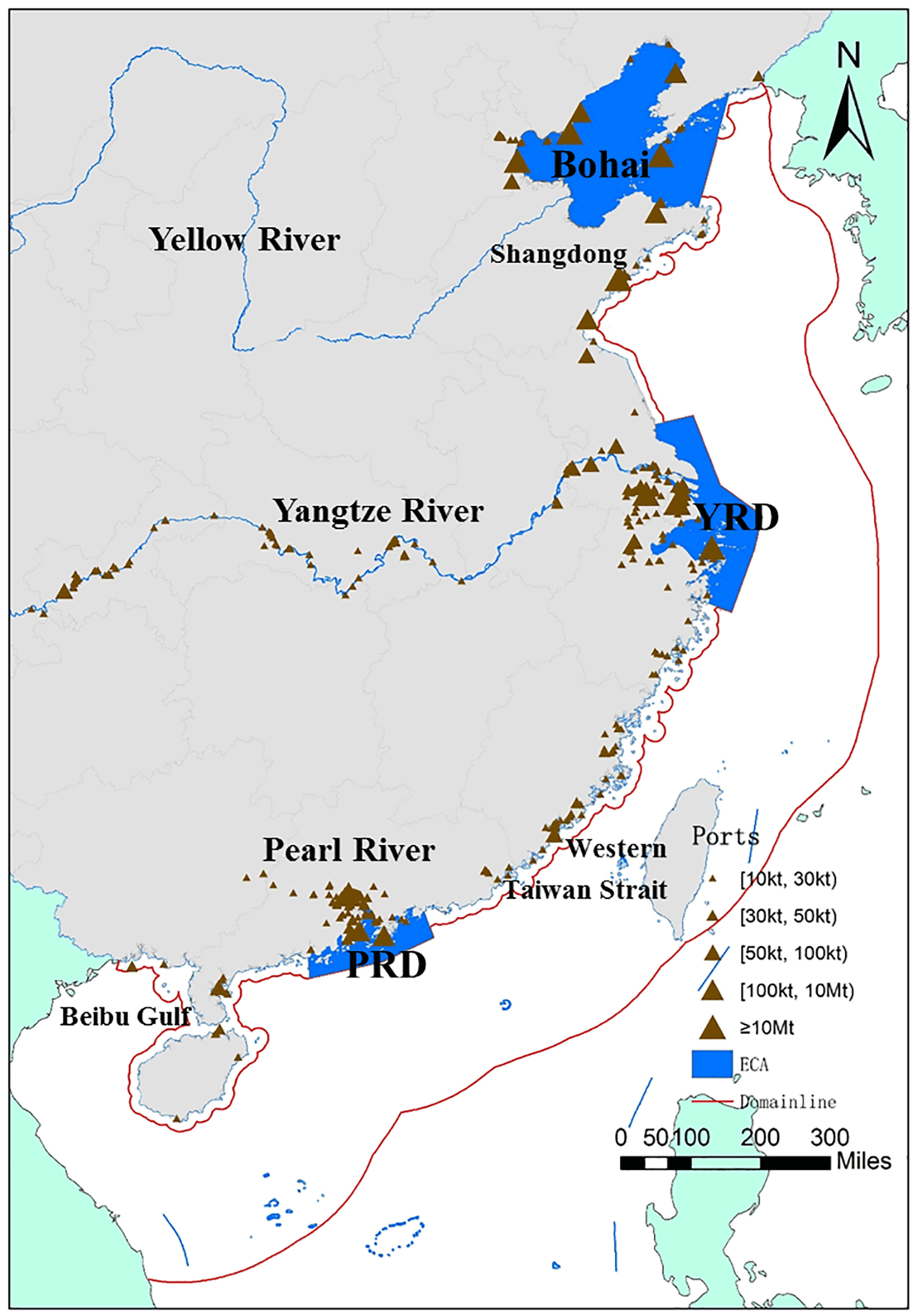
The study domain includes all ports in China and offshore waters within 200 Nm of the coast (17.93 to 41.82∘ N, 105.28 to 124.43∘ E). Based on the proposed DECAs and approved global ECAs approved by IMO (IMO, 2010, 2016), ship emissions within 12 and 200 Nm from the coastline of China, excluding offshore islands, were estimated (Fig. 1). To identify the transport distance and activity time in modes for ship emissions estimations, six port groups were defined geographically, namely Bohai, Shandong, Yangtze River Delta (YRD), Taiwan Strait, Pearl River Delta (PRD) and Beibu Gulf. The reason for choosing the 200 Nm offshore area as one of the research domains is to assess how the setting of ECAs influences emission reductions on shipping sources. More information about the domain is presented in Sect. 1 of the Supplement with Tables S1 and S2.
In this study, ships were classified by three classification schemes, namely OGVs, coastal vessels (CVs) and river vessels (RVs), as detailed in Table S3 in the Supplement. Four subcategories were classified by ship types, i.e., cargo ship, container, tanker, and others. Three subcategories were classified by ship flag and customs declarations to the marine department (MD) of China, i.e., OGVs operated under a foreign flag or engaged in international trade, CVs operated under the Chinese flag and not engaged in international trade, and RVs operated in the rivers and statistically independent of local MDs. Three subcategories were classified by operational modes, i.e., at sea, maneuvering and at berth (IMO, 2015), as indicated in Table S4 in the Supplement. Emissions from the main engine (ME), auxiliary engine (AE) and auxiliary boilers (AB) were considered. Ships that traveled through the research domain but did not call at any port in mainland China were not included, their major shipping routes were extracted from a real-time AIS digital map shown in Fig. S1 in the Supplement and their potential influence was analyzed in Sect. 2 of the Supplement.
2.2 Approach
2.2.1 Estimation approaches
Different emission estimation approaches were described for shipping emission inventories worldwide (Dalsøren et al., 2009), in East Asia (Liu et al., 2016) and on a regional scale (Li et al., 2016). In this study, an AIS-based integrated approach was established to identify emissions contributions and their historical trends. This approach integrated two AIS-based methods to address the problems of data availability and completeness. One is the port-based approach, which makes use of the AIS-based ship activity time in mode in 2013 to fill the data gap in port-based vessel calling number. This enables a detailed characterization of ship emissions and their uncertainties. The other is the cargo-based approach which used province-specific cargo volume data categorized by cargo type and trade type. By combining these activity data with the average distances of major navigation routes between ports obtained from an AIS-based digital map, the historical emissions can be estimated. The cargo-based approach considers the effects of trade type, ship type structure, fuel quality and port function on ship emissions. Meanwhile, cross-validation between different statistical methods ensures robust and reliable inventory estimates. Details of the two approaches are introduced in the following sections.
Port-based approach
The port-based approach calculates ship emissions based on engine activity, as shown by Eq. (1) (US EPA, 2000, 2008; Ng et al., 2012):
where i, j, k, l, m, and n represent a single voyage, engine type, pollutant, dead weight tonnage (DWT) class in ship type, activity mode, and total vessel arrived number, respectively. E is emission (g), VAN is the vessel arrived number, P is the average installed engine power (kW), LF is the average engine load factor, T is the average operation time in three activity modes (h), and EF is the emissions factor corresponding to the engine and fuel types (g kW−1 h−1).
In this equation, VANs were further divided into subcategories according to ship type and DWT. The engine power and load factors of the ME were estimated using the Propeller Law based on the relationship between the instantaneous speed and the design speed, together with the detailed technical information of the ship engine which has been widely used in the estimation of ship emissions (ICF international, 2009). Owing to the lack of information and similar propulsion ratios for AE and AB (Ng et al., 2012), the propulsion ratios and load factors for different ship types and operational modes were obtained from technical reports (US EPA, 2008; Starcrest Consulting Group, 2009). Due to the difference in the DWT subclass range and distribution of ship profile in different studies, adjustments were made for major ship types such that the AE and AB engine defaults better corresponded with the ship size and tonnage (Entec UK Limited, 2010; Ng et al., 2012). In addition, AE was assumed to be off when the ship speed was more than 8 kn (except for container and passenger ships), and those ships with diesel–electric engines were assumed not to use their boilers.
Table 1Time in mode for different ship types within 12 and 200 Nm of the coast (unit: h voyage−1).
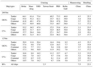
Table 2Transport distance for OGVs and CVs in different regions (unit: Nm).
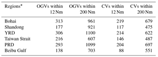
*The average transport distance of ships arriving in or departing from the corresponding port region.
An AIS-based ship trajectory was used to define the cruising time and maneuvering time for OGVs and CVs, which included the position, time, status, speed and course of ship. For RVs, the cruising time was calculated as the average transport distance divided by average ship speed, considering the main navigation routes in different regions. The hotelling time can be calculated using publicly available data regarding ship activity in the main ports of China, such as the ship name, ship type, destination harbors, departure times and arrival times (http://www.chinaports.com/). The calculation results are listed in Table 1. More information regarding emissions estimations is presented in the Supplement.
Cargo-based approach
A cargo-based approach considering the fuel consumption rate and transport distance is shown in Eq. (2):
where l, k, r, and m are ship type, pollutant, activity region and fuel type, respectively. Q is the transport volume (kt), TD is the average transport distance along the main navigation route (Nm), F is the fuel consumption rate (kg of fuel per kt Nm), and EF is the emissions factor (g kg−1 of fuel).
Transport volume, transport distance, fuel consumption rate and emission factor are therefore essential factors to estimate emissions in historical years. Transport volume is the real weight of transport cargo for a period of time. It was extracted from the annual report of 100 Chinese ports in 6 port clusters. Due to the lack of transport volume in different ship types, the stock of waterway cargo types in different provinces was separated into OGVs, CVs and RVs using the province-specific throughput of coastal ports and river ports, and it was then adjusted by the contributions of foreign trade in the main ports. Detailed transport volume data for all 100 ports is provided in Table S5 in the Supplement. Transport distance is the weight-based length along common ship routes of OGVs and CVs. Specifically, transport distances of OGVs were calculated as the average of the main international routes from the main ports in a particular port cluster, combined with the fraction of regular routes to South Korea, Japan, the South China Sea and the Pacific, respectively (Table S6 in the Supplement); transport distances of CVs were derived from transport distances between port clusters measured by the AIS data and digital map. We collected information of more than 1000 regular routes, including their departure and arrival ports (sample as Fig. S2b in the Supplement). We classified departure and arrival ports into port clusters, and then used the AIS data and digital map to calculate transport distances between port clusters. The calculation process of transport distances and AIS-based ship trajectories was shown in Fig. S2 in the Supplement. The calculation results are presented in Table 2. The determination of fuel consumption rate and emission factor is introduced in detail in Sects. 2.3.2 and 2.3.3, respectively.
Table 3Summary of ship calls number by marine department in 2013.
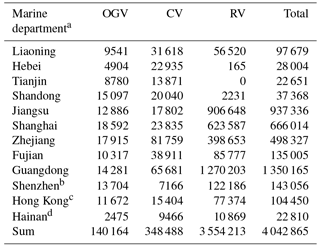
a Ordered from north to south China.
b The MD of Shenzhen was independent of the Guangdong
MD;
c Refers to the HKMD official website (H.K.EPD,
2015).
d The domain corresponding to statistics compiled
by the Hainan MD covered the ports in Hainan and Guangxi provinces.
2.2.2 Temporal and spatial allocation
Ship fuel consumption was temporally and spatially allocated using surrogates from AIS data and other official statistics. Because ship fuel consumption is significantly correlated with port throughput and main navigation routes, the average monthly throughput data in 2010–2013 were used to depict monthly variations in fuel consumption from container ships and cargo ships so as to account for the difference among annual variation caused by the fluctuations in international trade. As the weekly and daily variations of fuel consumption were very small, as illustrated in density distribution of AIS data (Fig. S3 in the Supplement), using 1 day if data per month can reproduce the monthly variation of fuel consumption well. As we did not have hourly cargo transport data, diurnal variation of fuel consumption was determined based on AIS ship track data.
A dot-density-weighted algorithm was applied for the spatial allocation of emissions. This algorithm used the density of data “dots” to calculate spatial surrogates by weighting emissions from different pollutant types and navigation modes. The emissions in different ports and water areas were defined based on hotelling and cruising information. According to the weights of the above spatial surrogates in every grid cell, the ship emissions were distributed in 3 km × 3 km grid cells covering the research domain.
2.2.3 Uncertainty
Previous studies indicated that the uncertainties in ship emissions were mainly introduced by time in mode, load factors and emission factors (Yang et al., 2007; Ng et al., 2013), but these uncertainties were not quantified. In this study, AIS data were used to quantitatively characterize the uncertainties associated with time in modes and load factors using a bootstrap simulation approach. Statistical methods and expert judgment were used to estimate uncertainties in the emission factors. The uncertainty ranges of emission factors and time in modes are presented in Tables S7 and S8 in the Supplement, respectively. Using a Monte Carlo simulation approach, the propagation of uncertainties in the above inputs into the estimated results was evaluated. This quantitative assessment revealed key contributors of uncertainties, which called attention to the need for further inventory improvement and refinement.
2.3 Data sources and validation
2.3.1 Port distribution and ship activity
To ensure the reliability and precision of the emissions estimates, verification of the input data is important. Here, the difference in input data from different data sources was analyzed, and the potential reasons for the variations were discussed. Specifically, data at the national level, provincial level and port level from different statistical departments, e.g., National Bureau of Statistics, MD and Port Association, were compared. Other parameters in the port-based approach, including vessel call, ship type stock, engine power, load factor and activity time in mode, were also examined.
Table 3 lists the vessel calls based on MDs. The difference between the statistics provided by the national MD and some local MDs might be caused by the existing differences in statistical methods and different classifications of vessel calls, e.g., regular shipment, international trade, domestic trade and local shipment. To address these differences, port-based vessel calls were summarized based on 11 regional MDs defined by the Ministry of Transport of China (MD Report, 2015, unpublished) using the same statistical approach. The RV data were obtained directly and solely from the national MD. As the ship statistics by MD were not classified based on DWT, an adaptive sampling approach based on real-time AIS data was adopted by considering port sizes and wharf structures to remove errors in individual sampling periods. A summary of the stock of ship types that navigated in different regions is presented in Fig. S4 in the Supplement. The detailed data sources are shown in Fig. S5 in the Supplement.
The activity information for different ship types was collected from various sources. Information for more than 5000 OGVs and CVs was acquired from Lloyd's Register of Ships (LRS). Registration information regarding nearly 7600 RVs was acquired from local MDs. Liu et al. (2016) reported that almost 18 000 ships navigated in the East Asian seas, which supported the representativeness of samples used in this study. The LRS and MD registration databases provided the registration number, ship type and tonnage, major sea routes, fuel type, engine information, and other relevant information for emissions estimates.
Specifically, approximately 700 AIS-based navigation trajectories with all data from 2013 were collected, including 350 million AIS messages with 3 million operation hours covering OGVs, CVs, RVs and major ship types. In comparison with the AIS dataset in East Asia for 2013 (Liu et al., 2016), the area of the research domain in this study was around 71 % and covered 69 % of ship information, including all regular routes. This meant that the density of ship information in this study was comparable with Liu et al. (2016). Based on this AIS dataset, ship activity profiles were established by considering different regions, ship types and size categories, e.g., time in modes, load factors and spatiotemporal surrogates. More information regarding the AIS data is presented in Table S9 in the Supplement.
2.3.2 Cargo transport trends and fuel consumption statistics
Based on the cargo transport statistics, there were no significant differences between different statistical departments, such as the China Port Statistics Yearbook (CPSY, 2004–2014), China Statistics Yearbook, and Statistics Communique of China on the Traffic and Transportation Industry Development (CCTD, 2008–2015). Because CPSY provides both national and provincial cargo transport balances and covers OGVs, CVs and RVs on the provincial scale, transport volume balances were adopted for estimation from 2004 to 2013. Transport volume of cargo types in 6 port clusters with 100 Chinese ports from 2004 to 2013 were shown in Table S5a–k in the Supplement; more information about transport volume was shown in the Supplement..
The fuel consumption rates of OGVs and CVs used in this study were based on the median values of the range provided by the IMO report (IMO, 2015), and they accounted for the differences between container, general cargo, bulk carrier and tanker ships; for RVs, the value of 5.2 tce per 10 kt was provided by the CCTD. More information regarding fuel consumption rates is presented in Fig. S6 in the Supplement.
2.3.3 Emission factors
Apart from activity data, pollutant emission factors are also imperative for emission inventory development. Emission factors were described per kilowatt hour (Li et al., 2016; Fan et al., 2016; Liu et al., 2016) and per kilogram of fuel consumption (Jin et al., 2009; Bao et al., 2014) in different studies. To make emission factor units from the literature consistent and to analyze their uncertainties, a fuel consumption rate of 227 g kWh−1 was calculated for heavy fuel oil (HFO) and a rate of 217 g kWh−1 was calculated for marine diesel oil (MDO) and gas oil (Ng et al., 2012). In China, most RV engines were produced by Chinese manufacturers, such as Zichai, Weichai and Guangchai. Therefore, the average values of emission factors obtained via field measurements on local ships were used in this study (Zhang et al., 2016).
Table 4Sulfur transfer rates of different engine types used in this study.
* Calculated based on the average values reported in previous studies.
Table 5Ship emissions reduction analysis scenarios of SO2 DECA and NOx DECA.
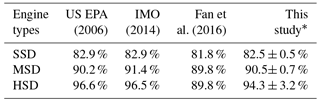
Given that the marine ship industry is associated with international trade and technology, there are no significant differences in ship engine emissions for OGVs. To reduce the uncertainties in emissions estimates due to emission factors, the relationships between emission factors by pollutant and ship characteristics, such as engine type, fuel type, sulfur content and emissions standards, were identified using a quantitative assessment approach. In this study, SO2 emissions were calculated using both the sulfur balance approach and the sulfur transfer rate, which were dependent upon the engine type (US EPA, 2008; IMO, 2016; Fan et al., 2016). As indicated in Table 4, sulfur contents of fuel consumption for OGVs, CVs and RVs were determined by considering the global average value (IMO, 2016) and the local and national statistical values (Fan et al., 2016). The global background values of sulfur contents used for estimation are shown in Fig. S7 in the Supplement. To assess the historical and future trends of NOx emissions under control policies with different NOx emission standards, NOx emission factors under different influence factors were determined from the IMO study (IMO, 2015) and Liu et al. (2016), as detailed in Table S10 in the Supplement. Emissions of particulate matter, hydrocarbon (HC), CO, black carbon (BC) and organic carbon (OC) were determined based on the engine types and fuel types (US EPA, 2006, 2009; Zhang et al., 2016), as shown in Table S11 in the Supplement. All emission factors were selected according to local emission characteristics for navigational areas, ship types and DWT values, as listed in Table S12 in the Supplement. Low-load adjustment multipliers were applied when the load factors of ME were below 20 % to account for the low combustion correction coefficient during low main engine loading conditions (ICF International, 2009), as indicated in Table S13 in the Supplement.
Table 6Comparison of HFO consumption in China in 2013 (unit: kt).
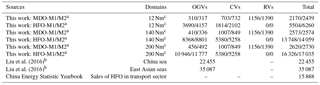
a M1/M2 represent cargo-based and port-based approach, respectively; MDO and HFO represent marine diesel oil and marine heavy oil. b Calculated using CO2 emissions and an emission factor of 3591.12 g CO2 kg−1 of Fuel (IMO Report, 2015). c The distance to Chinese shore.
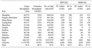
Table 7Port activity and fuel consumption in the top 10 ports in China.
2.3.4 Control scenarios and factors for emission projection
Ship emissions in China are largely associated with international trade patterns and ship engine technology development. Future ship emissions are therefore determined by multiple factors, including trade and political (e.g., DECA, emissions standard), economic (e.g., gross domestic product (GDP), shipbuilding industry), social (e.g., sulfur content of HFO, population), and technological (e.g., engine type, after-treatment devices) factors. In this study, fuel consumption was used to predict baseline ship emission scenarios since there are strong associations between fuel consumption and ship emissions (Fig. S8 in the Supplement), and emission control scenarios were used to adjust baseline emissions under different control strategies.
Changes in ship fuel consumption at 5-year intervals from 2015 to 2040 in China were estimated by the output data from a predication model with high reliability (IEA, 2016). Specifically, estimation of marine fuel consumption in 2013 was used as the base-year value. Fuel consumption associated with inland and coastal navigation sources (oil and gas) were used to predict fuel consumption of CVs and RVs, whereas international marine bunkers were used to predict fuel consumption of OGVs.
Table 8Summary of ship emissions in China (within 200 Nm of the coast) in 2013.
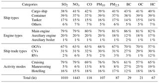
Table 9Uncertainties in emission estimates.
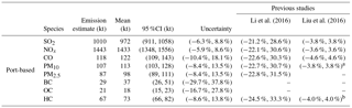
a Results of PM. b Results of NMVOC.
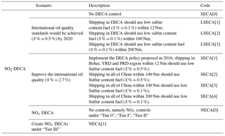
A total of 10 scenarios were designed for SO2 and NOx emissions reductions based on a global sulfur cap of 0.5 % by 2020 as planned by the IMO. Because NOx emission reductions depend on new engine technologies such as exhaust gas recirculation (EGR), selective catalyst reduction (SCR) and liquefied natural gas (LNG) engines, a 20-year lifetime for ship engines was assumed for the engine renewal period. Current legislation and DECAs were factored into the scenarios. Additional emissions control policies targeting SO2 and NOx emissions from vessels and ports were evaluated based on emissions reductions, including a baseline, SO2 DECA (SECA) and NOx DECA (NECA), as detailed in Table 5. Future emissions were calculated at 5-year intervals.
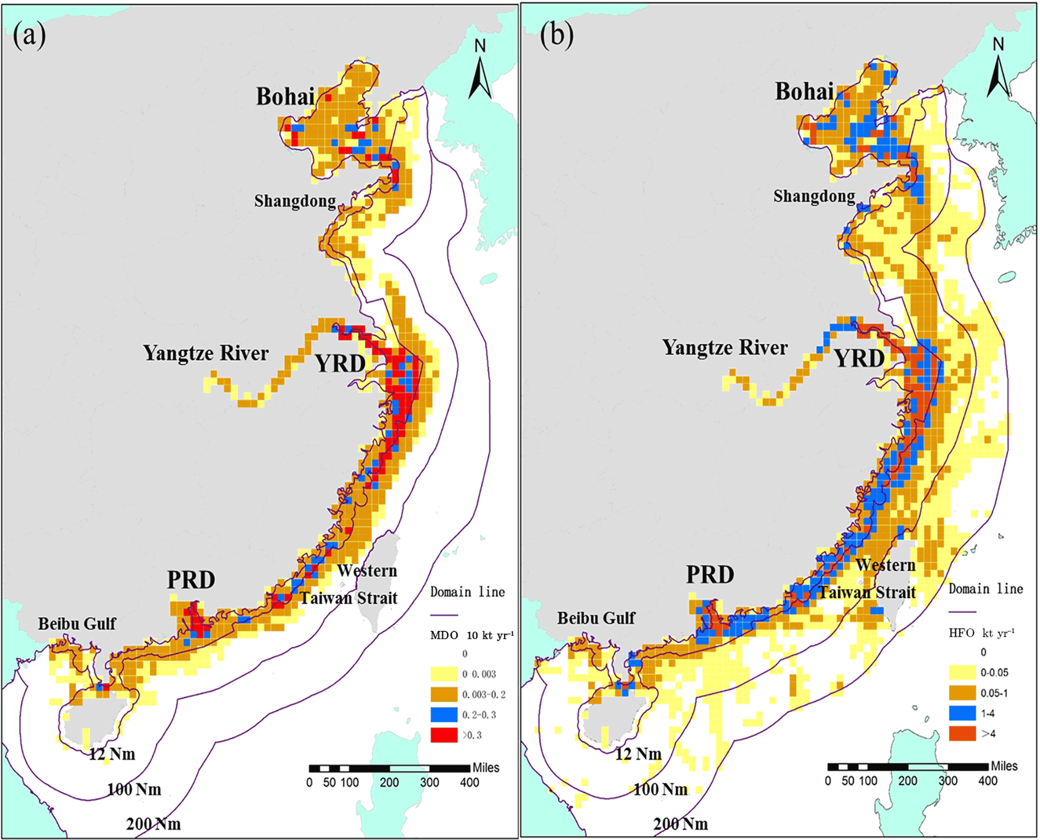
Figure 2Spatial distribution of marine diesel oil MDO (a) and HFO (b) consumption by ships (27 km × 27 km).
3.1 Characteristics of ship emissions in 2013
3.1.1 Estimation of fuel consumption in ports and sea
In 2013, there was no ship emission control measure in China. Ship emissions were therefore largely determined by fuel consumption. We start this section by discussing fuel consumption characteristics in ports and at sea which can be indicative of and verify ship emissions in 2013.
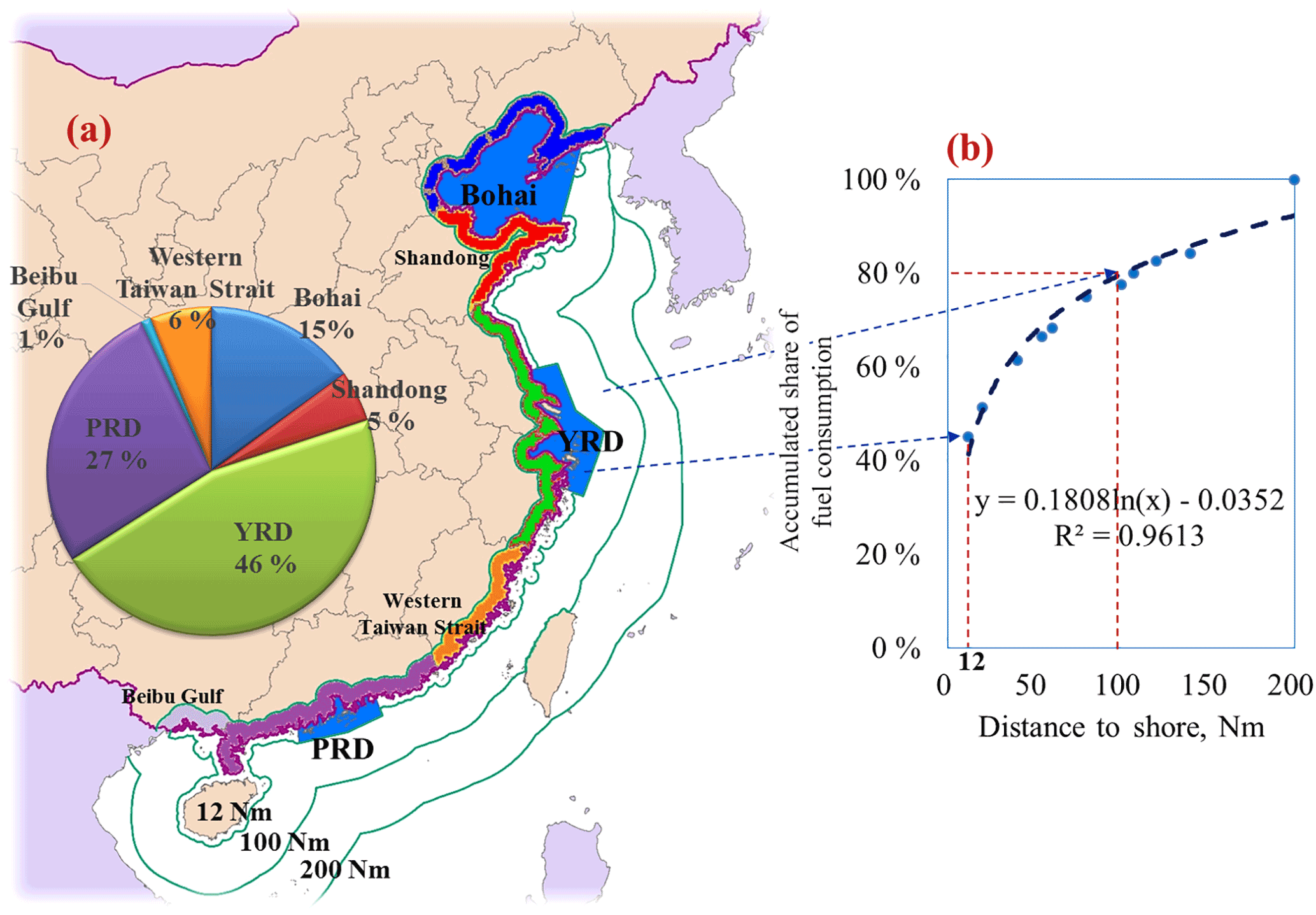
Figure 3(a) Fuel consumption contributions of different port groups within 200 Nm and (b) the cumulative distribution of fuel consumption within 200 Nm.
The integrated approach is used to estimate ship fuel consumption in China in 2013, as shown in Table 6. Total fuel consumption based on port-based and cargo-based approaches exhibited a good agreement within 12 and 200 Nm of the coastline (deviation < 15 %). More than 85 % of MDO was consumed within 12 Nm, and almost 80 % was contributed by RVs and CVs, particularly by RVs. Conversely, only 35 % of HFO was consumed within 12 Nm, and OGVs dominated its consumption. Although there were differences in the MDO estimations of CVs and RVs between two approaches, they were mainly associated with small CVs that were categorized as RVs in port under the port-based approach. Here, the results of the port-based approach were used for comparison. Total fuel consumption within 200 Nm was estimated to be 17 035 kt in 2013, within which 2730 kt of MDO was consumed in rivers and coastal waters. Fuel consumption in the overlapping area estimated by Liu et al. (2016) was almost 25 % greater than that in this study because of differences in domain size and estimation approach.
Table 10Emission intensities in three DECAs and along typical navigation lines.
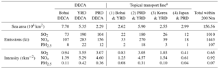
* Geographic location of transport lines shown in Fig. S9 in the Supplement.
Figure 2 showed the spatial allocation maps of MDO and HFO, which were calculated by the dot density of AIS data from RVs and CVs within 50 Nm and from OGVs within 200 Nm of the coastline, respectively. As most MDO was consumed by RVs and low-power CVs, the spatial distribution of MDO follows the coastline and rivers, especially in the YRD region. OGVs predominantly consume HFO, therefore the highest densities of HFO appear in the development areas of international trade and near the international navigation routes, such as the YRD, PRD, Bohai and regular routes connecting YRD and PRD.
We further examined the port activity and fuel consumption for the top 10 ports in China, as detailed in Table 7. The results indicated that Shanghai and Ningbo-Zhoushan contributed to ∼ 28 % of total HFO consumption; Hong Kong, Shenzhen and Guangzhou contributed 23 %, whereas 36 % of total HFO was consumed outside the top 10 ports. HFO consumption in all ports accounted for ∼ 30 % of the total ship fuel consumption within 12 Nm. In comparison, nearly 70 % of the total MDO was consumed within 12 Nm of the top 10 ports, and 42 % was consumed in ports. Shanghai, Guangzhou and Suzhou were the largest MDO consumption ports in China (43 % of the total MDO), as a great number of RVs were operated in the dense waterways of the YRD and PRD. It is interesting to note that the ranks of ship fuel consumption were not the same as those of cargo throughput, container throughput and vessel arrived number. The difference was mainly caused by port conditions and target clients, which further causes huge differences in emissions from different ship types. Using cargo throughput, container throughput or vessel arrived number to represent ship emissions would therefore generate misleading results. Our results suggest that the consideration of ship type and DWT is crucial for accurate estimation of ship emissions.
Previous studies reported a strong correlation between emissions and the distance from the coastline in the YRD region (Fan et al., 2016; Liu et al., 2016). In this study, by taking advantage of the port-based approach, fuel consumption of ocean traffic can be determined in a designated port, and fuel consumption from different coastal port clusters can be identified. As shown in Fig. 3a, HFO consumption from the YRD, PRD and Bohai regions accounted for more than 85 % of the total consumption in China, with YRD itself accounting for 46 %. This provides solid evidence for the DECAs in these three regions proposed by the Chinese government in 2016. Figure 3b shows the cumulative distribution of HFO with the distance to the coastline, which indicated that the DECAs within 12 Nm covered about 40 % of the HFO from the total ship sector within 200 Nm and can reach 80 % when the distance was extended to 100 Nm.
3.1.2 Compilation of ship emission inventory and uncertainty
Based on the above fuel consumption results, the ship emission inventory in 2013 in China was calculated by combining with a fuel-based emission factor. Table 8 lists ship emissions within 200 Nm of the coastline in 2013. Emissions of SO2, NOx, PM10, PM2.5, CO and HC were 1010, 1443, 118, 107, 87 and 67 kt yr−1, respectively. Compared with the total anthropogenic emissions in MEIC (Li et al., 2014; Zheng et al., 2014; Liu et al., 2015), emissions from ships accounted for about 10 % of the total SO2 emission and 9 % of the total NOx emission from all sectors in coastal provinces. Cargo ships (general cargo ships and dry bulk carriers), container ships and tankers (chemical tankers, gas tankers and oil tankers) were the main contributors of all pollutants, accounting for 38–42, 37–39 and 14–17 % of total pollutants emitted within 200 Nm of the coast, respectively. These results are in line with previous estimates (Liu et al., 2016). The AE was responsible for 20 % of SO2 and NOx, similar to 26 % in East Asia (Liu et al., 2016) but significantly higher than the global fraction of 10 % (Paxian et al., 2010) and lower than 40–60 % from local ports or regions (Ng et al., 2013; Fan et al., 2016; Li et al., 2016). These diversified results mainly resulted from ship navigating time in cruising mode in different research domains, and the simplifications on basic parameters of AE and AB, e.g., lower output power of cargo ships and container ships in this study than those in Liu et al. (2016). We also noted that RVs contributed to 6 % of NOx and 2 % of SO2 in the shipping sector, which was not reported in previous studies. The majority of ship emissions occurred during ship cruising, whereas ship emissions at berth and during maneuvering only comprised 14 and 5 % of total ship emissions, respectively.
Table 9 summarizes the estimated means and the associated uncertainty ranges of pollutant-based ship emissions in 2013 using Monte Carlo methods. CO emission showed relatively large uncertainties, ranging from 109 to 143 kt in the 95 % confidence interval with relative errors of −10 to 18 %. In comparison, the uncertainties in SO2 and NOx were relatively small, ranging from 991 to 1058 kt and from 1348 to 1556 kt, respectively, with relative errors of −6 to 9 % in the 95 % confidence intervals. The high uncertainties in CO estimates were mainly caused by the differences in emission factors from different sources (US EPA, 2006; ICF International, 2009; Liu et al., 2016), which varied between engine type, combustion conditions and operation modes. Overall, the uncertainties reported in this study were larger than those reported in large-scale studies (∼ ±5 %) and lower than those in small-scale studies (∼ ±20 %) (Li et al., 2016; Liu et al., 2016).
3.1.3 Temporal characteristics
Figure 4 shows the monthly and diurnal variations of emissions from different ship types. Based on the temporal surrogates of container and cargo transport in the southern (south of YRD) and northern (north of YRD) port groups from 2010 to 2013, the monthly variations in container and cargo ship emissions were similar, with small variations. Additionally, emissions were slightly higher in August and December and lower in February. This was mainly due to increased ship activity in the summer and winter, with relatively less cargo transport during the long public holiday of Spring Festival in February. These variations were generally consistent with some local studies (Ng et al., 2013; Li et al., 2016) but differed from Fan et al. (2016), which indicated that ship emissions were the highest in April and no significant differences in total emissions were observed in June, November and December. Passenger ships exhibited a bimodal monthly variation pattern, with peaks in August and December.
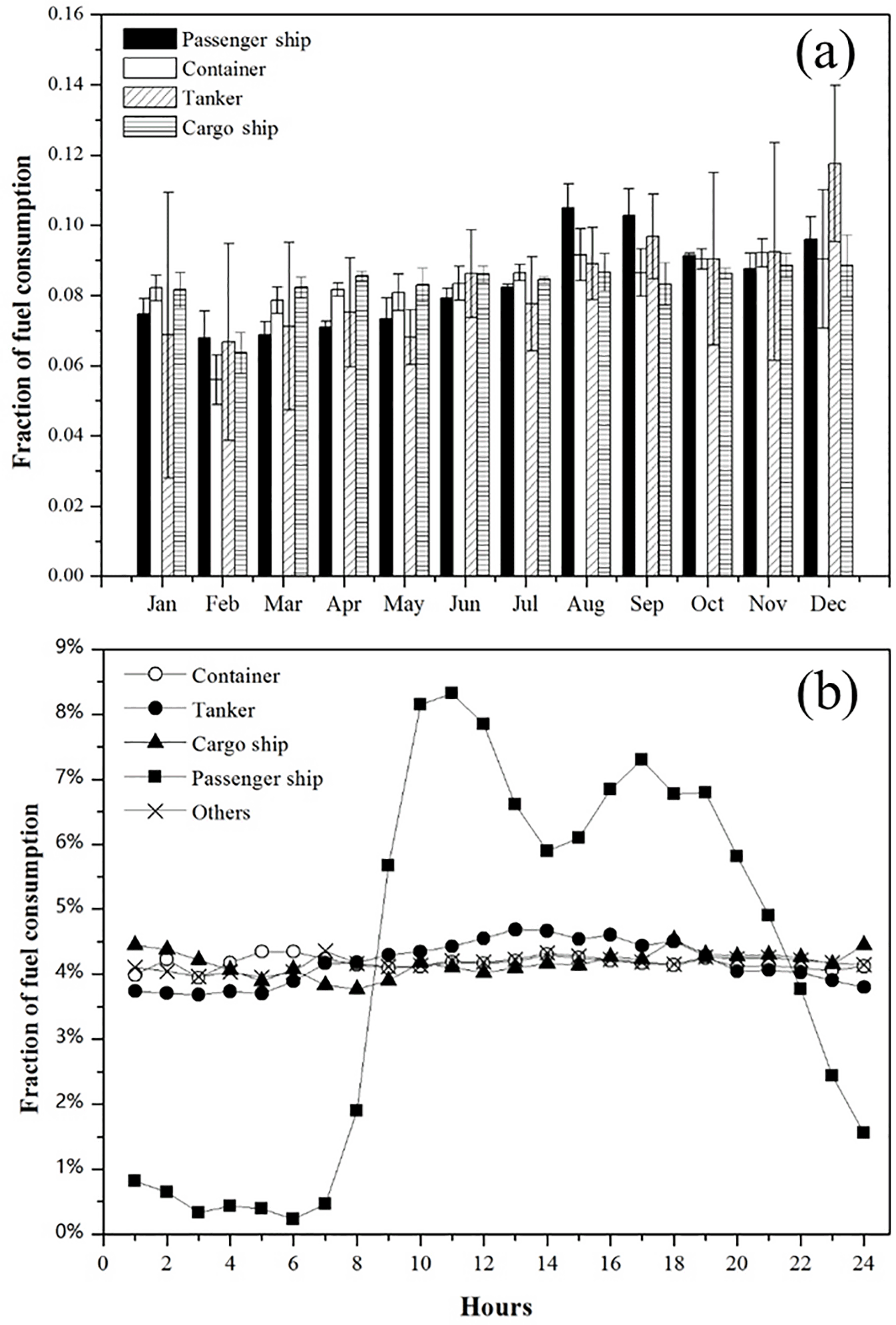
Ferries were the only type that exhibited significant diurnal patterns. With an hourly percentage of less than 1 % at midnight and in the early morning, fuel consumption from ferries increased dramatically starting at 08:00 LT, reached a peak at 10:00–11:00 LT, then slightly declined and reached another peak at 17:00 LT. Fuel consumption from other ship types remained constant over the course of a day because these ships were generally used for long-distance transport and sailed at all times under the 24 h rotation system.
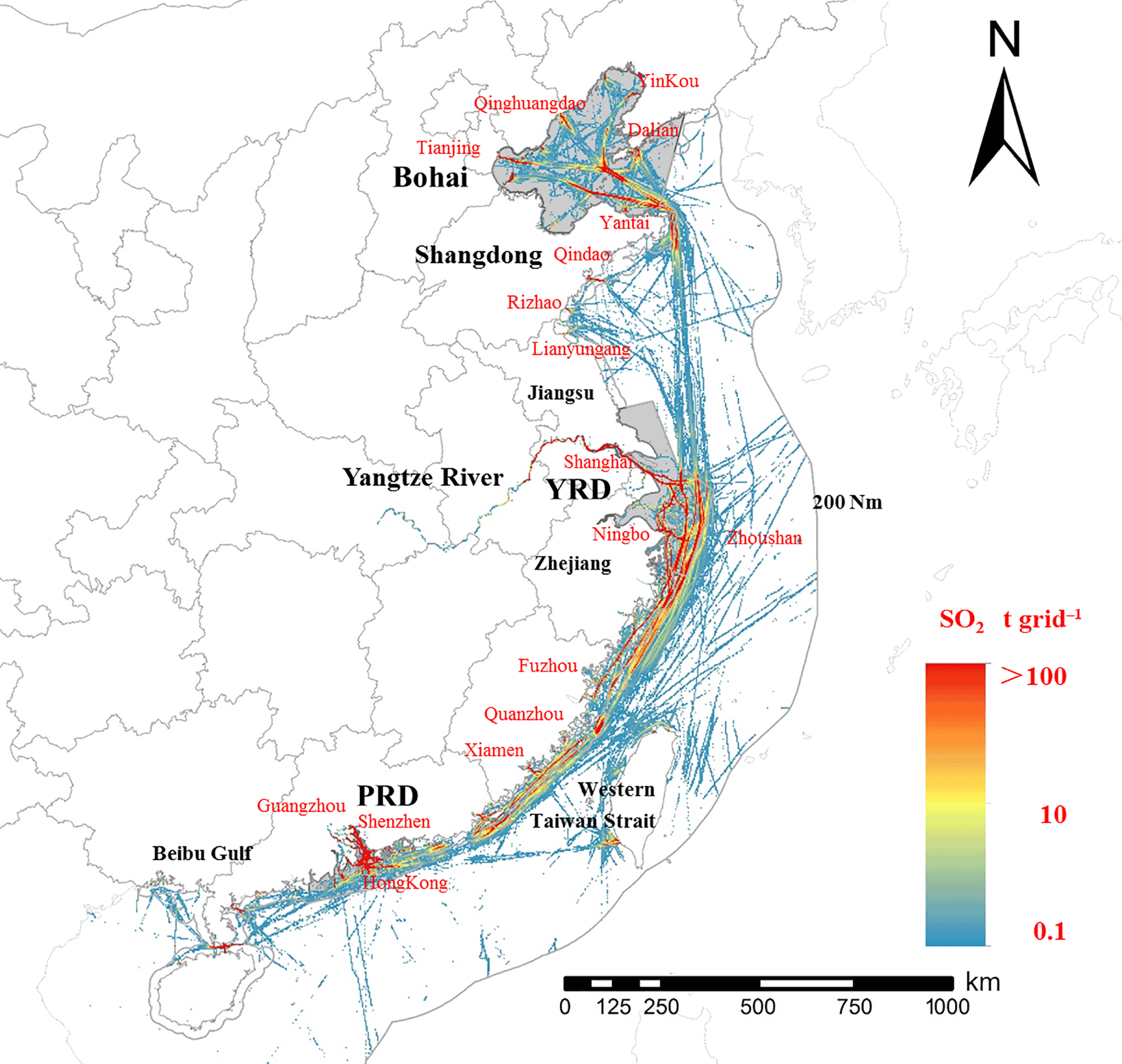
3.1.4 Geographic distribution and emissions intensity
Figure 5 shows the spatial allocation of SO2 (3 km × 3 km) in the ship emission inventory in 2013, with the main ports and navigation routes highlighted. It is clear that the emission distribution is strongly consistent with the current regular navigation routes. Specifically, the lines south of YRD are more aggregated, whereas those north of YRD were more scattered and concentrated in the ports of Dalian, Tianjin and Qingdao and the transport routes in between, as shown in Fig. S9 in the Supplement. By contrast, the emissions over the PRD were concentrated on the lines to the north and in the estuary. Because the YRD region is a fast-developing international shipping center and the convergence area of the south and north waterways, the emissions were very intensive in this region.
Previous studies showed that ship emissions were commonly concentrated, and ship emissions from different geographical areas, such as traffic hubs (Fan et al., 2016), ports (Ng et al., 2013), coastal areas (Ng et al., 2012; Goldsworthy et al., 2015; Li et al., 2016) and the sea (Jalkanen et al., 2009; Tournadre et al., 2014; Liu et al., 2016), were discussed. In this study, special analysis was conducted with regard to emissions from DECAs and typical shipping routes in China.
Table 10 presents the emission intensities of SO2, NOx and PM10 in three DECAs and along four typical shipping routes (Fig. S9 in the Supplement). The results indicated that all DECAs and shipping routes contributed significant emissions to coastal waters. Only covering 19 % of the total area within 200 Nm, the DECAs and shipping routes contributed to almost 36–38 and 27–29 % of total emissions, respectively. As YRD DECA has the highest traffic concentration in East Asia, the average intensities of SO2, NOx and PM2.5 emissions were 6 times those of East China Sea (Liu et al., 2016). With three busy ports (Hong Kong, Guangzhou and Shenzhen), the intensity of PRD DECA was approximately 8 times higher than average emission intensities of the South China Sea (Liu et al., 2016). A previous study indicated that emission values greater than 8 t yr−1 km−2 were common in the busy fairways of the East China Sea (Fan et al., 2016), but the values associated with traffic hubs are still ambiguous. Table 10 presents the SO2, NOx and PM2.5 emission intensities at four traffic hubs along shipping routes. The route between the YRD and PRD (including the Taiwan Strait) is one of the busiest sea routes in the world, and the emission intensities were similar to those in the PRD DECA and much greater than those of the Bohai DECA. By contrast, the sum of emissions intensities of the other three regular routes were slightly less than the route between the YRD and PRD as they became scattered to the Bohai, South Korea and Japan.
3.2 Ship emissions from 2004 to 2013
3.2.1 Trends in ship activities
Figure 6 shows the multiyear estimation of HFO consumption in main port clusters within 200 Nm offshore using a cargo-based approach from 2004 to 2013. HFO consumption in China increased from 8040 kt in 2004 to 17 035 kt in these 10 years, with an annual growth rate of 9 %. This change has been driven by the rapid increase in international trade (10 % growth in the external trade of cargo) due to the economic boom (10 % growth in GDP) during this period.

Figure 6Trends in HFO consumption in port clusters in China from 2004 to 2013: (a) fuel consumption and (b) normalized fuel consumption.
Although fuel consumption had more than doubled from 2004 to 2013, the growth of cargo and container turnover in most port groups were even more significant (Fig. S10 in the Supplement). We expect the difference would become even larger as a result of technological development of the diesel engine in the future. In addition, the growth rate of top-scale port clusters (PRD and Shanghai) were relatively lower than others. Specifically, traffic in the Jiangsu and Liaoning port clusters even recorded an almost five-fold increase. Such a significant increase was largely contributed by the dramatic growth of domestic trade in China, which highlighted the urgent need for emission control on RVs and CVs. There was a slight drop in traffic in 2008 amid the general increase trend in these 10 years, which was largely caused by the declined external trade in most ports in China resulting from the global economic crisis (Fig. S11 in the Supplement).
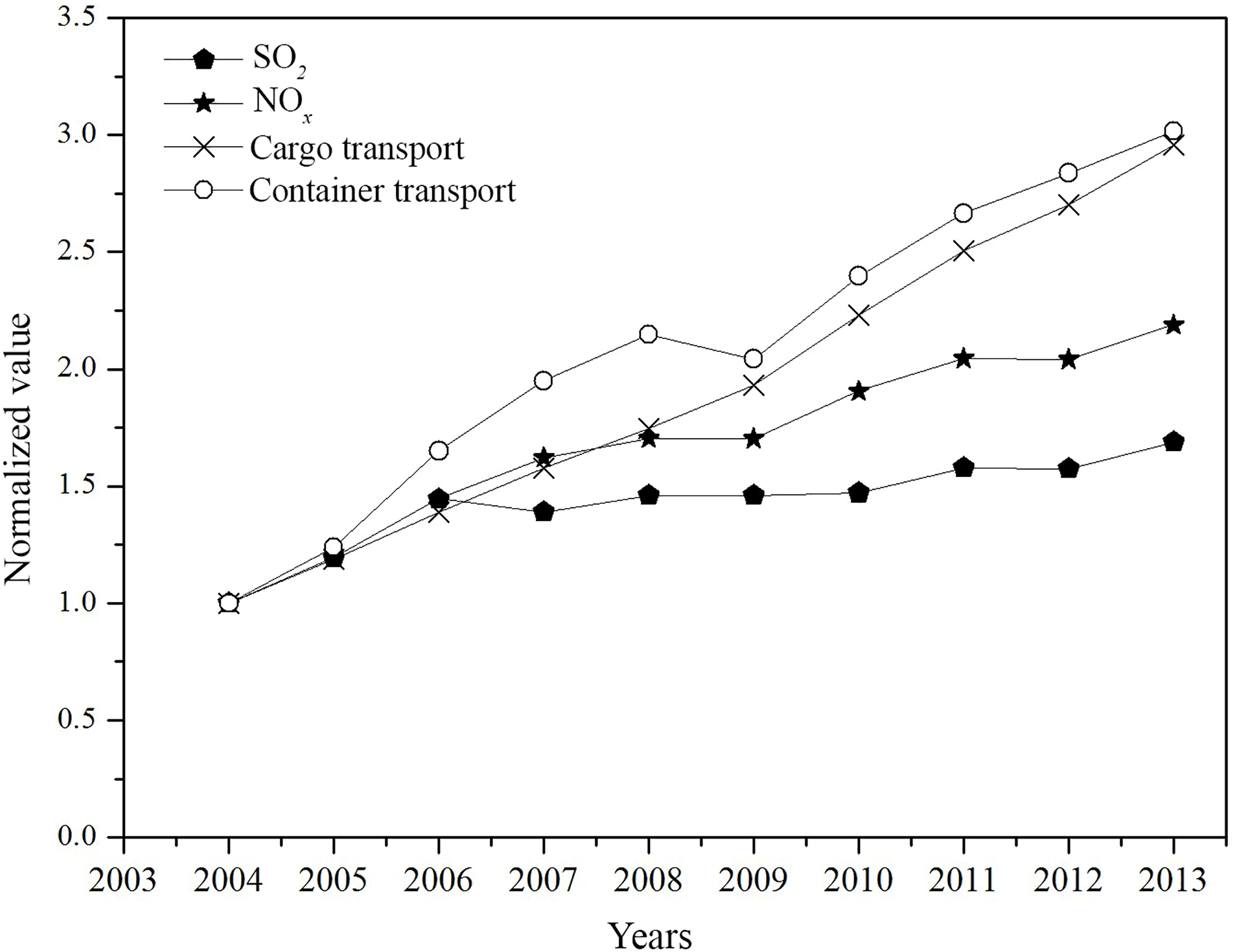
Figure 7SO2 and NOx emissions and their aggregated emissions from cargo and container transport from 2004 to 2013.
3.2.2 Emission trends
Figure 7 uses SO2 and NOx as examples to show the trends of ship emissions in China from 2004 to 2013. The results indicated that emissions increased first, leveled off or even decreased slightly in 2008 and 2009, and then increased rapidly afterwards. The drop in 2008 was mainly caused by decreased container turnover due to a weakened international trade market during the international financial crisis. This period was followed by a rapid increase with the global economic recovery after 2009. During these 10 years, seaborne trade for both cargo and container transport in China tripled, but the increase in pollutant emission was slower, e.g., 1.7 times for SO2 and 2.2 times for NOx. The low growth rate of SO2 compared to that of NOx emissions was caused by the improvement in the sulfur content of global HFO from 3.5 to 2.7 % over the past 10 years (Fig. S7 in the Supplement). In comparison, emission factors of NOx decreased slightly due to technological difficulties in further improving ship engines. The increasing trends for SO2 and NOx were different from those for land-based anthropogenic sources. SO2 emissions from power plants and other major sources have decreased substantially since 2005 due to the application of emissions control technologies (Lu et al., 2010), and NOx emissions declined continuously after 2011 (Zhao et al., 2013).
3.3 Estimation of ship emissions during 2013–2040
3.3.1 Impacts of various SO2 DECA policies
Figure 8a shows SO2 emission reductions based on the global sulfur cap of 0.5 %, and the results indicated that SO2 emissions will be reduced by over 80 % when the 0.5 % sulfur cap is achieved in 2020. Emissions can be further reduced by 86, 91 and 94 % within 12, 100 and 200 Nm, respectively, by expanding DECA regions with 0.1 % sulfur content in oil. These results indicated the importance of lowering the sulfur content of global marine oil.
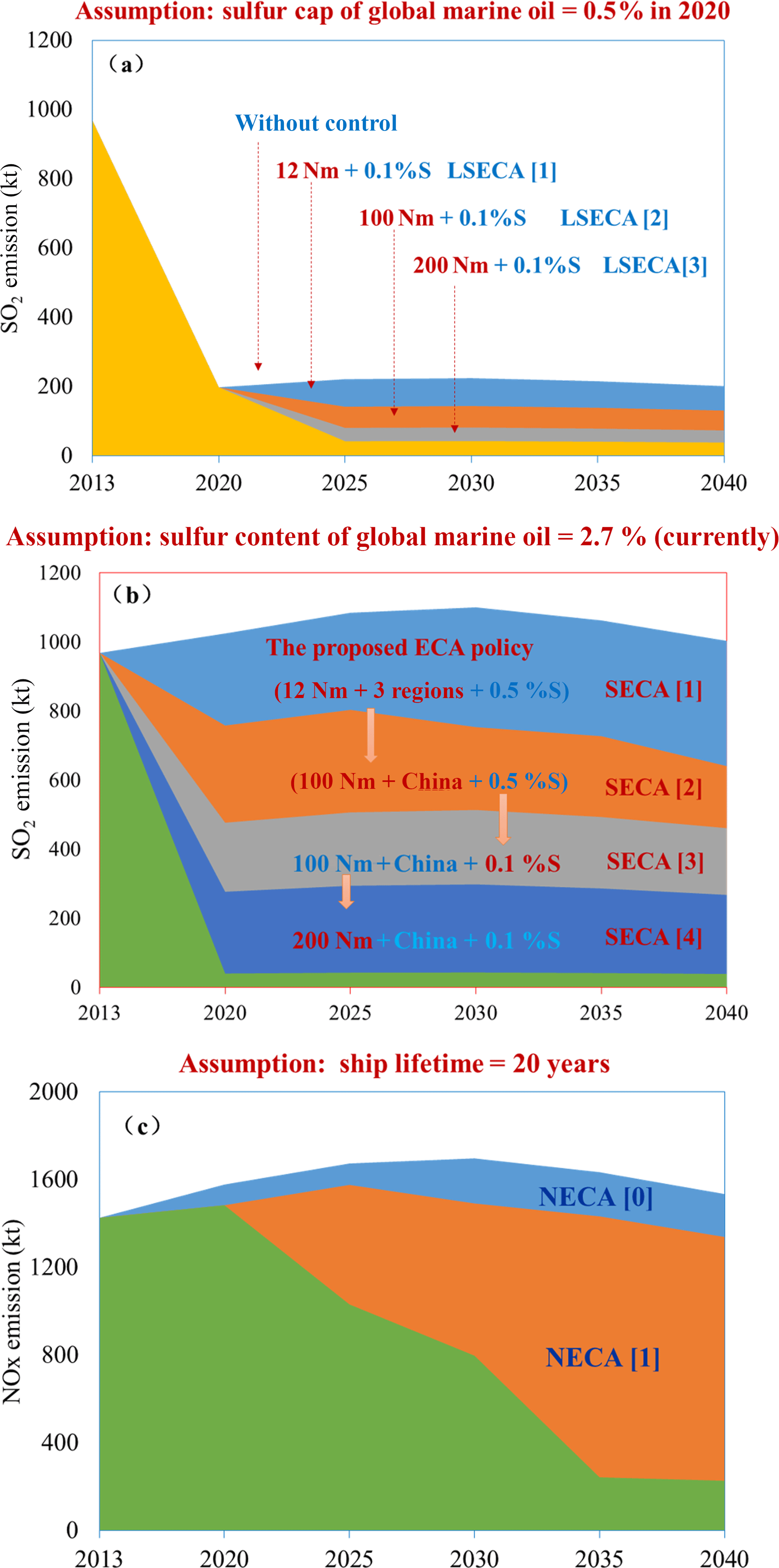
Figure 8SO2 and NOx emissions from the shipping sector under SO2 DECA (a, b) and NOx DECA (c) with different control policies from 2013 to 2040.
If the 0.5 % global sulfur cap fails to achieve, China could make its own effort to reduce SO2 emission from ships, as shown in Fig. 8b. The proposed DECA policy within 12 Nm in three regions can reduce SO2 emissions by over 20 %. Further scenarios with different DECA strategies were calculated from 2020 to 2040. SO2 emissions can be reduced by over 50 % by expanding the DECA regions to within 100 Nm of the entire Chinese coast and using 0.5 % sulfur content fuel. An additional 25 % reduction is expected by expanding the DECA to 200 Nm and using 0.1 % sulfur content fuel. In total, 94 % of SO2 emissions can be mitigated.
3.3.2 Impacts of NOx DECA policies
Currently, the effective approaches for limiting NOx emissions from ships depends on the development of new ship engines, such as EGR, LNG and SCR engines. Thus, reductions in NOx emissions were associated with passive step-by-step controls if no enforcement measures were implemented for existing ships. Therefore, the assumption of a 20-year ship lifetime was used in this study. Figure 8c shows future NOx emissions with or without a NOx DECA in China. If there is no emissions control plan for “Tier III” ship engines, the emission from engines with “Tier II” NOx emission standards will peak in 2030, and with the elimination of “Tier 0” ship engines, a 13 % reduction in NOx emissions can be achieved by 2040. By contrast, if China implements a NOx DECA within 200 Nm of China coastline in 2020, NOx emissions can be reduced by 80 %.
4.1 Implications for policy making
This study showed a significant increase in ship emissions in China from 2004 to 2013, which highlighted the urgent need for effective control of ship emissions. Application of cleaner fuels and environmentally friendly ship engines are possible means to reduce ship emissions in China. This study also provided justifications for the establishment of DECAs in China.
To improve regional air quality and facilitate the structural adjustment of industry, an implementation plan for DECAs in the waters of the Bohai, YRD and PRD regions was established in December 2015. This was a health-based initiative that is anticipated to have positive long-term effects on those who live and work in DECAs and nearby. Shanghai as a demonstration city has observed positive impact after implementation of this policy for 1 year. However, many issues still may hinder successful implementation of the policy. We believe the following tasks are essential:
-
More technical guidelines and standards regarding the exhaust emissions of ships and the use of shore power and other clean energy, e.g., supervision guidelines for DECAs, should be issued.
-
Qualitative and quantitative emissions management should be improved by strengthening monitoring procedures, responsible parties and managers should be quickly spotted, and the illegal emissions of air pollutants from ships should be banned.
-
Smooth communication and regional cooperation should be enhanced, e.g., communication with shipping and energy enterprises to increase the supply of low-sulfur fuel and offset shipping costs in cooperation with multiple environmental authorities for joint prevention and control.
-
Awareness from different stakeholders should be enhanced, e.g., alleviation of community and public attention, strengthening social responsibility of governments and corporations, optimization of standardized management and service function, and investment in public health mechanisms in port areas.
-
future phases of emissions control policies should be formulated, e.g., enhancement of the DECA policy from local to regional, national and continental scales based on scientific findings to formulate both short-term and long-term effective ship emission control strategies.
4.2 Call for more comprehensive data
We used an integrated AIS-based methodology to represent the characteristics and trends of ship emissions in China. In this methodology, it was assumed that the empirical statistics of voyages along regular routes and in ports were correlated with the ship type and geography and that emission factors changed along with changes in oil quality and engine technology. Uncertainty in ship activity parameters and emissions factors will impact the accuracy of the emissions characteristics and trends. Discrepancies in total ship emissions existed in global-, regional- and port-scale studies. The key reason for the emissions discrepancies was not only the uncertainty in annual activity rates and emission factors but also the quality of different data sources and variations in the assumptions underlying different methods. For example, the Ports of Los Angeles and Long Beach (PoLa) study assumed that the ship AE was shut down when the ship speed exceeded 8 kn (except for passenger ships; Starcrest Consulting Group, 2009; Ng et al., 2013), but there were other studies assuming that the AE worked all the time (IMO, 2015; Liu et al., 2016). Additionally, BEs were used on OGVs in the IMO study but were not included in ships with diesel-electric engines in the PoLa study.
Moreover, the estimation of emissions factors were characterized in most studies, but some studies only considered fuel type and engine type (Fan et al., 2016). Some studies also ignored missing ships in the AIS dataset (Ng et al., 2013; Li et al., 2016). Due to uncoordinated control policies in different regions and the poor performance of the port environmental statistics system in China, field surveys and measurements must be conducted, more accurate local assumptions must be made and a standardized methodology for estimating ship emission inventories is needed.
Small differences in the assumptions can yield large errors in the emission estimates. To avoid this problem, we suggest maximizing the collaboration with other related entities (e.g., engine manufacturers, regulatory agencies, port authorities, vessel owners, the published literature and commercial entities) to gain a more complete and unbiased understanding, fill data gaps, and mutually validate approaches. Subsequently, plans to conduct field surveys and measurements to establish local databases and validate these assumptions should be made. Examples include the engine operation conditions of different ship types under local navigational conditions (especially under the current national emissions reduction framework), the tendency of fuel quality and engine technology, and the integrity and accuracy of the real-time data obtained from the AIS dataset.
To establish a standardized methodology for estimation, some suggestions are proposed:
-
fill the data gap and optimize data quality by implementing various measures, e.g., data integrity and volume checks, data longevity assessment, separation of real data from assumptions or defaults, separation of activity-based values from those based on factors or equipment, provision of valid data ranges for factors and equipment, improvement in geospatial data collection, and establishment of quality assurance and quality control (QAQC) measures;
-
standardize data collection procedures, verify the existing results, conduct third party reviews of findings and update existing inventories with these findings;
-
develop a regulatory framework, e.g., cross-comparison datasets, which limit interpretation errors, evaluate data quality and perform data logging and emissions testing; and
-
conduct vessel boarding programs to collect actual vessel and operational parameters, e.g., equipment duty cycle; engine operation; fuel use and fuel switching data; main, auxiliary and boiler loads according to mode; and operational parameters according to mode.
A robust emissions inventory is essential for planning and tracking as environment challenges broaden. Thus, further refinement of ship emission inventories should be conducted to ensure regulatory emissions inventories are accurate and to track the progress of emissions reductions strategies. In addition, because coastal areas in China are densely populated, more assessment studies should be conducted based on reliable emission inventories to develop sustainable, cost-effective, environmental and human health solutions, e.g., health risk assessments, air quality assessments and cost–benefit evaluations of control policies.
We demonstrated a good agreement in ship emissions estimation by AIS-based integrated approach based on different data sources, and these results provided solid evidence for better understanding national-, regional- and local-scale ship emissions in China. The results indicated that ship emissions within 200 Nm of the Chinese coast were 1010, 1443, 118, 107, 87, 67, 29 and 21 kt yr−1 for SO2, NOx, PM10, PM2.5, CO, HC, BC and OC in 2013, respectively. Ship emissions constituted approximately 10 % of the total NOx and SO2 emissions in coastal cities. Approximately 40 % of the pollutants from ships were emitted within 12 Nm of the coast, and would be doubled within a distance of 100 Nm. Therefore, the expansion of the DECAs could greatly improve the control effect. YRD, PRD and Bohai Regions contributed 46, 27 and 15 % to the total HFO emissions, respectively. Additionally, about 65 % of ship emissions came from the top 10 ports, which also contributed to 24 % of the total emissions within 200 Nm. In addition to the proposed DECAs, more attention should be paid to the emissions along regular navigational lines near coastlines, especially the Taiwan Strait and south–north routes. Furthermore, ship emissions have doubled over the past 10 years, and SO2 DECA and NOx DECA control policies can potentially achieve > 80 % emission reductions in the future. For NOx, similar reductions could be achieved via strict engine emissions controls, low-sulfur fuel oil and a switch to propulsion with natural gas. However, such policies would not provide substantial benefits until 2040 because decades are needed to implement fleet-wide changes. Potential reduction efforts are of considerable regional importance because ship emissions along the Chinese coast account for almost half of the total ship emissions in East Asia.
This study established a methodology in using limited AIS data to develop ship emission inventory. Such a methodology can be used in other parts of the world, as most of the time it is not possible to collect a complete set of AIS information. The emission estimation and uncertainty analysis in this study have great reference values for modelers and other emission inventory users. The AIS-based spatial and temporal allocation methods have great representativeness and could well satisfy the simulation requirement by the models.
The data can be accessed upon request to the corresponding author.
The supplement related to this article is available online at: https://doi.org/10.5194/acp-18-6075-2018-supplement.
The authors declare that they have no conflict of interest.
This work was supported by the National Distinguished Young Scholar Science
Fund of the National Natural Science Foundation of China (41325020), Public
Environmental Service Project of the Ministry of Environmental Protection of
People's Republic of China (201409012) and the Chinese National Member
Organization at the International Institute for Systems Analysis, Laxenburg,
Austria. Edited by: Jianzhong Ma
Reviewed by: three anonymous referees
Bandemehr, A., Muehling, B., Corbett, J., Comer, B., and Boyle, J.: U.S.-Mexico cooperation on reducing emissions from ships through a Mexican emission control area: development of the first national Mexican emission inventories for ships using the waterway network ship traffic, energy, and environmental model (STEEM), Office of International and Tribal Affairs, EPA-160-R-15-001, available at: https://www.epa.gov/nscep, May 2015.
Bao, X., F., Ding, Y., Yin, H., Huang, Z. H., Wang, J. F., and Ma, D.: Guideline of method for emissions estimation from non-road mobile source. available at: http://www.qhepb.gov.cn/xwzx/zqyj/201407/W020140711608259681099.pdf, 2014.
China National Ports Association, China Port Statistics Yearbook (CPSY), available at: http://navi.cnki.net/KNavi/YearbookDetail?pcode=CYFD&pykm=YZGAW&bh=, 2004–2014.
Corbett, J. J. and Koehler, H. W.: Updated emissions from ocean shipping, J. Geophys. Res.-Atmos., 108, 87–107, 2003.
Corbett, J. J., Windebrake, J. J., Green, E. H., Kasibhatla, P., Eyring, V., and Lauer, A.: Mortality from ship emissions: a global assessment, Environ. Sci. Technol., 24, 8512–8518, 2007.
Dalsøren, S. B., Eide, M. S., Endresen, Ø., Mjelde, A., Gravir, G., and Isaksen, I. S. A.: Update on emissions and environmental impacts from the international fleet of ships: the contribution from major ship types and ports, Atmos. Chem. Phys., 9, 2171–2194, https://doi.org/10.5194/acp-9-2171-2009, 2009.
Endresen, O., Sorgard, E., Sundet, J. K., Dalsoren, S. B., Isaksen, I. S. A., Berglen, T. F., and Gravir, G.: Emission from international sea transportation and environmental impact, J. Geophys. Res., 108, 4650–4665, https://doi.org/10.1029/2003JD003751, 2003.
Endresen, O., Sørgard, E., Behrens, H. L., and Brett, P. O.: A historical reconstruction of ships' fuel consumption and emissions, J. Geophys. Res., 112, D12301, https://doi.org/10.1029/2006JD007630, 2007.
Fan, Q. Z., Zhang, Y., Ma, W. C., Ma, H. X., Feng, J. L., Yu, Q., Yang, X., Ng, S. K. W., Fu, Q. Y., and Chen, L. M.: Spatial and seasonal dynamics of ship emissions over the Yangtze River Delta and East China Sea and their potential environmental influence, Environ. Sci. Technol., 50, 1322–1329, https://doi.org/10.1021/acs.est.5b03965, 2016.
Fu, Q. Y., Shen, Y., and Zhang, J.: Study on ship emission inventory in Shanghai port, J. Safety Environ., 12, 57–63, 2012.
Fu, L., Wang, W., Zhang, W. H., and Cheng, H. H.: Air Quality in China in 2016 the process of air pollution prevention and control, CLEAN AIR ASIA, available at: http://www.allaboutair.cn/uploads/160816/airchina2016.rar, 2016.
Goldsworthy, L. and Goldsworthy, B.: Modelling of ship engine exhaust emissions in ports and extensive coastal waters based on terrestrial AIS data – an Australian case study, Environ. Model. Software, 63, 45–60, https://doi.org/10.1016/j.envsoft.2014.09.009, 2015.
He, C. F., Xu, T., Hu, Q. Y., and Ge, Y. D.: Acquisition of ship AIS data via Beidou satellite navigation system. Journal of Shanghai Maritime University, 34, 5–9, 2013.
Hong Kong Environment Protection Department (H.K.EPD): Ocean going vessels fuel switch at berth, available at: http://www.epd.gov.hk/epd/sites/default/files/epd/english/environmentinhk/air/guide_ ref/files/Leaflet% 20for% 20Fuel% 20Switch% 20at% 20Berth% 20Regulation% 20English.pdf, 2015.
ICF international: Current Methodologies in Preparing Mobile Source Port-related Emission Inventories, Final Report, 2009.
International Energy Agency (IEA): World Energy Outlook Special Report 2016: Energy and Air Pollution, available at: https://webstore.iea.org/world-energy-outlook-2016, 2016.
International Maritime Organization (IMO): Information on North American Emission Control Area under MARPOL ANNEX VI, available at: http://www.doc88.com/p-9485203363727.html, May 2010.
International Maritime Organization (IMO): Third IMO Greenhouse Gas Study 2014 Executive summary and Final Report, available at: https://www.researchgate.net/publication/281242722_Third_IMO_GHG_Study_2014_Executive_Summary_and_Final_Report, 2015.
International Maritime Organization (IMO): Marine Environment Protection Committee (MEPC), 70th session, available at: http://www.imo.org/en/MediaCentre/IMOMediaAccreditation/Pages/MEPC-70.aspx, 2016.
Jalkanen, J.-P., Brink, A., Kalli, J., Pettersson, H., Kukkonen, J., and Stipa, T.: A modelling system for the exhaust emissions of marine traffic and its application in the Baltic Sea area, Atmos. Chem. Phys., 9, 9209–9223, https://doi.org/10.5194/acp-9-9209-2009, 2009.
Jalkanen, J.-P., Johansson, L., and Kukkonen, J.: A comprehensive inventory of ship traffic exhaust emissions in the European sea areas in 2011, Atmos. Chem. Phys., 16, 71–84, https://doi.org/10.5194/acp-16-71-2016, 2016.
Jin, T., Yin, X., Xu, J., Yang, L., Ge, W., and Ju, M.: Air pollutants emission inventory from commercial ships of Tianjin Harbor, Marine Environ. Sci., 28, 623–625, 2009.
Li, C., Yuan, Z. B., Ou, J. M., Fan, X. L., Ye, S. Q., Xiao, T., Shi, Y. Q., Huang, Z. J., Ng, S. K. W., Zhong, Z. M., and Zheng, J. Y.: An AIS-based high-resolution ship emission inventory and its uncertainty in Pearl River Delta region, China, Sci. Total Environ., 573, 1–10. https://doi.org/10.1016/j.scitotenv.2016.07.219, 2016.
Li, M., Zhang, Q., Streets, D. G., He, K. B., Cheng, Y. F., Emmons, L. K., Huo, H., Kang, S. C., Lu, Z., Shao, M., Su, H., Yu, X., and Zhang, Y.: Mapping Asian anthropogenic emissions of non-methane volatile organic compounds to multiple chemical mechanisms, Atmos. Chem. Phys., 14, 5617–5638, https://doi.org/10.5194/acp-14-5617-2014, 2014.
Liu, F., Zhang, Q., Tong, D., Zheng, B., Li, M., Huo, H., and He, K. B.: High-resolution inventory of technologies, activities, and emissions of coal-fired power plants in China from 1990 to 2010, Atmos. Chem. Phys., 15, 13299–13317, https://doi.org/10.5194/acp-15-13299-2015, 2015.
Liu, H., Fu, M. L., Jin, X. X., Shang, Y. Shindell, D., Faluvegi, G., Shindell, C., and He, K. B.: Health and climate impacts of ocean-going vessels in East Asia, Nat. Clim. Change, 6, 1037–1041, https://doi.org/10.1038/NCLIMATE3083, 2016.
Lu, Z., Streets, D. G., Zhang, Q., Wang, S., Carmichael, G. R., Cheng, Y. F., Wei, C., Chin, M., Diehl, T., and Tan, Q.: Sulfur dioxide emissions in China and sulfur trends in East Asia since 2000, Atmos. Chem. Phys., 10, 6311–6331, https://doi.org/10.5194/acp-10-6311-2010, 2010.
Ministry of Transport of China: Implementation plan on domestic Emission Control Areas in waters of the Pearl River Delta, the Yangtze River Delta and Bohai Rim (Beijing, Tianjin, Hebei), 2015-01183, available at: http://zizhan.mot.gov.cn/zfxxgk/bzsdw/bhsj/201512/P020160215528398838765.pdf, 2015.
Ng, S. K. W., Lin, C., Chan, J. W. M., Yip, A. C. K., Lau, A. K. H., and Fung, J. C. H.: Study on marine vessels emission inventory, Final Report, Civic Exchange, 1–20, 2012.
Ng, S. K. W., Loh, C., Lin, C., Booth, V., Chan, J. W. M., Yip, A. C. K., Li Y., and Lau, A. K. H.: Policy change driven by an AIS-assisted marine emission inventory in Hong Kong and the Pearl River Delta, Atmos. Environ., 76, 102–112, 2013.
Paxian, A., Eyring, V., Beer, W., Sausen, R., and Wright, C.: Present-day and future global bottom-up ship emission inventories including polar routes, Environ. Sci. Technol., 44, 1333–1339, 2010.
Schrooten, L., De Vlieger, I., Panis, L. I., Chiffi, C., and Pastori, E.: Emissions of maritime transport: a European reference system, Sci. Total Environ., 408, 318–323, 2009.
Song, S.: Ship emissions inventory, social cost and eco-efficiency in Shanghai Yangshan port, Atmos. Environ. 82, 288–297, 2014.
Starcrest Consulting Group: The Port of Los Angeles Inventory of Air Emissions for Calendar year 2008, Technical Report, ADP# 050520-525, available at: https://www.portoflosangeles.org/DOC/REPORT_Air_Emissions_Inventory_2009.pdf, 2009.
Tan, J. W., Song, Y. N., Ge, Y. S., Li, J. Q., and Li, L.: Emission inventory of ocean-going vessels in Dalian Coastal area, Res. Environ. Sci., 27, 1426–1431, 2014.
Tournadre, J.: Anthropogenic pressure on the open ocean: the growth of ship traffic revealed by revealed by altimeter data analysis, Geophys. Res. Lett. 41, 7924–7932, 2014.
US Environmental Protection Agency (US EPA): Analysis of commercial marine vessels emissions and fuel consumption data, EPA420-R-00-002, 2000.
US Environmental Protection Agency (US EPA): Control of Emissions from Marine SI and Small SI Engines, Vessels, and Equipment, EPA420-R-08-014, 2008.
Wang, C. F., Corbett, J. J., and Firestone, J.: Improving spatial representation of global ship emissions inventories, Environ. Sci. Technol., 42, 193–199, https://doi.org/10.1021/es0700799, 2008.
Whall C., Scarbrough T., Stavrakaki A., Green C., Squire T. and Noden R.. Entec UK: Limited UK ship emissions inventory, Final Report, available at: https://uk-air.defra.gov.uk/assets/documents/reports/cat15/1012131459_21897_Final_Report_291110.pdf, 2010.
Yang, D. Q., Kwan, S. H., Lu, T., Fu, Q. Y., Cheng, J. M., Streets, D. G., Wu, Y. M., and Li, J. J.: An emission inventory of marine vessels in Shanghai in 2003, Environ. Sci. Technol., 41, 5183–5190, 2007.
Yang, J., Yin, P. L., Ye, S. Q., Wang, S. S., Zheng, J. Y., and Ou, J. M.: Marine emission inventory and its temporal and spatial characteristics in the city of Shenzhen, Environ. Sci., 36, 1217–1226, 2015.
Yau, P. S., Lee, S. C., Corbett, J. J., Wang, C. F., Cheng, Y., and Ho, K. F.: Estimation of exhaust emission from ocean-going vessels in Hong Kong, Sci. Total Environ., 431, 299–306, 2012.
Ye, S. Q., Zheng, J. Y., Pan, Y. Y., Wang, S. S., Lu, Q., and Zhong, L. J.: Marine emission inventory and its temporal and spatial characteristics in Guangdong Province, Acta Sci. Circumst., 34, 537–547, 2014.
Zhao, B., Wang, S. X., Liu, H., Xu, J. Y., Fu, K., Klimont, Z., Hao, J. M., He, K. B., Cofala, J., and Amann, M.: NOx emissions in China: historical trends and future perspectives, Atmos. Chem. Phys., 13, 9869–9897, https://doi.org/10.5194/acp-13-9869-2013, 2013.
Zhang, F., Chen, Y., Tian, C., Lou, D., Li, J., Zhang, G., and Matthias, V.: Emission factors for gaseous and particulate pollutants from offshore diesel engine vessels in China, Atmos. Chem. Phys., 16, 6319–6334, https://doi.org/10.5194/acp-16-6319-2016, 2016.
Zheng, B., Huo, H., Zhang, Q., Yao, Z. L., Wang, X. T., Yang, X. F., Liu, H., and He, K. B.: High-resolution mapping of vehicle emissions in China in 2008, Atmos. Chem. Phys., 14, 9787–9805, https://doi.org/10.5194/acp-14-9787-2014, 2014.