The importance of vertical resolution in the free troposphere for modeling intercontinental plumes

Zhuang, Jiawei; Jacob, Daniel J.; Eastham, Sebastian D.

doi:https://doi.org/10.5194/acp-18-6039-2018

Articles | Volume 18, issue 8

https://doi.org/10.5194/acp-18-6039-2018

Articles | Volume 18, issue 8

Research article

02 May 2018

Research article |

| 02 May 2018

The importance of vertical resolution in the free troposphere for modeling intercontinental plumes

Jiawei Zhuang, Daniel J. Jacob, and Sebastian D. Eastham

Abstract

Chemical plumes in the free troposphere can preserve their identity for more than a week as they are transported on intercontinental scales. Current global models cannot reproduce this transport. The plumes dilute far too rapidly due to numerical diffusion in sheared flow. We show how model accuracy can be limited by either horizontal resolution (Δx) or vertical resolution (Δz). Balancing horizontal and vertical numerical diffusion, and weighing computational cost, implies an optimal grid resolution ratio (Δx ∕ Δz)_opt ∼ 1000 for simulating the plumes. This is considerably higher than current global models (Δx ∕ Δz ∼ 20) and explains the rapid plume dilution in the models as caused by insufficient vertical resolution. Plume simulations with the Geophysical Fluid Dynamics Laboratory Finite-Volume Cubed-Sphere Dynamical Core (GFDL-FV3) over a range of horizontal and vertical grid resolutions confirm this limiting behavior. Our highest-resolution simulation (Δx ≈ 25 km, Δz ≈ 80 m) preserves the maximum mixing ratio in the plume to within 35 % after 8 days in strongly sheared flow, a drastic improvement over current models. Adding free tropospheric vertical levels in global models is computationally inexpensive and would also improve the simulation of water vapor.

Download & links

Article (PDF, 4655 KB)

Supplement (13075 KB)

Download & links

Article (4655 KB)
Supplement (13075 KB)
BibTeX
EndNote

How to cite

How to cite.

Dates

Received: 04 Dec 2017 – Discussion started: 08 Dec 2017 – Revised: 10 Apr 2018 – Accepted: 10 Apr 2018 – Published: 02 May 2018

1 Introduction

Global transport of pollution mainly takes place in the free troposphere where winds are strong and pollutant lifetimes are long. The free troposphere extends from the top of the planetary boundary layer (PBL, typically 2 km altitude) up to the tropopause. It is a prevailingly stable environment with strong wind shear. Much of pollution transport in the free troposphere takes place as plumes, typically ∼ 1 km thick in the vertical, that fan out horizontally over a ∼ 1000 km scale and may preserve their coherent structure for up to 1–2 weeks (Newell et al., 1999; Stoller et al., 1999; Thouret et al., 2000; Heald et al., 2003; Crawford et al., 2004; Liang et al., 2007). Global Eulerian models dilute these plumes too rapidly because of numerical diffusion introduced by the advection schemes. Although the high-order advection schemes used in models are highly accurate under uniform flows, the accuracy breaks down in realistic sheared/stretched flows where plumes filament, and the ability to resolve cross-plume gradients is rapidly compromised (Rastigejev et al., 2010). Eastham and Jacob (2017) found that increasing the horizontal resolution of models to address this problem is only of marginal benefit and suggested that the main limitation is vertical resolution. Here, we use the Geophysical Fluid Dynamics Laboratory Finite-Volume Cubed-Sphere Dynamical Core (GFDL-FV3), a global 3-D dynamical core that explicitly solves atmospheric dynamic equations, to understand the horizontal and vertical resolution requirements for models to simulate global-scale plume transport.

Preserving the structure of chemical plumes during global-scale transport is important for representing non-linear chemical and aerosol processes (Wild and Prather, 2006) and for quantifying intercontinental influences on surface air (Lin et al., 2012; Zhang et al., 2014). For example, models are unable to capture the plumes of Asian ozone pollution frequently observed at 2–5 km altitude over California (Hudman et al., 2004; Nowak et al., 2004). Air quality agencies in California have claimed that they cannot meet the current surface ozone standard because of this Asian pollution influence (Neuman et al., 2012). Models find Asian pollution influence in surface air over California to be only a few ppb (Goldstein et al., 2004; Zhang et al., 2008), but since they cannot resolve the structure of Asian pollution plumes crossing the Pacific they have little credibility.

General circulation models (GCMs) used for global simulations of atmospheric dynamics including meteorological data assimilation have increased their resolutions 1000-fold over the past 50 years, buoyed by the growth of computing power (Balaji, 2015). Increasing horizontal resolution has been privileged, and attention to vertical resolution has mainly focused on the PBL. For example, assimilated meteorological data produced operationally by the NASA Goddard Earth Observing System (GEOS) started in the 1990s with 2^∘ × 2.5^∘ horizontal resolution and 20 vertical levels (GEOS-1; Schubert et al., 1993). Today, the operational GEOS forward processing (GEOS-FP) product uses a cubed-sphere C720 horizontal resolution (≈ 0.125^∘) and 72 vertical levels (Lucchesi, 2017). This represents a 20-fold increase in horizontal resolution but only a 4-fold increase in vertical resolution. In the free troposphere at 2–10 km altitude, the vertical resolution has increased by only a factor of 2 from GEOS-1 (8 levels) to GEOS-FP (15 levels). In NOAA's Next Generation Global Prediction System (NGGPS) program, several state-of-the-science dynamical cores are tested at horizontal resolutions of 12 km and 3 km but only with 128 vertical layers – not trying to improve on the current generation of models (Michalakes et al., 2015). ECMWF's Integrated Forecasting System (IFS) increased its horizontal resolution from 16 km to 9 km in 2016 but its vertical resolution remains at 137 levels (Haiden et al., 2016). On the Sunway TaihuLight supercomputer, a dynamical core is tested at an unprecedentedly high global horizontal resolution of 488 m but with only 128 vertical layers (Yang et al., 2016).

There are important reasons why horizontal resolution is a priority in GCMs, as reviewed by Haarsma et al. (2016). Increasing horizontal resolution improves the simulation of large-scale features such as the El Niño–Southern Oscillation (ENSO), as well as small-scale features such as tropical cyclones. It has been argued that increasing vertical resolution should follow suit. Pecnick and Keyser (1989) recommend an optimal relationship between horizontal and vertical grid spacing to resolve fronts:

\begin{matrix} (1) & {(\frac{Δ x}{Δ z})}_{opt} = \frac{1}{s}, \end{matrix}

where s is the frontal slope, and Δx and Δz are the horizontal and vertical grid spacings, respectively. s typically ranges from 0.005 to 0.02 for synoptic-scale fronts, so the optimal Δx ∕ Δz would be in the range 50–200. Lindzen and Fox-Rabinovitz (1989) recommend the following equation for resolving quasi-geostrophic flows:

\begin{matrix} (2) & {(\frac{Δ x}{Δ z})}_{opt} = \frac{N}{f}, \end{matrix}

where N is the Brunt–Väisälä frequency and f is the Coriolis parameter. N∕f ∼ 100 is Prandtl's ratio, measuring the ratio between the horizontal and vertical scales of geostrophic flows (Dritschel and McKiver, 2015). Based on both Eqs. (1) and (2), Δx ∕ Δz in GCMs is recommended to be of the order of 100 (Chapter 3.2.1 of Warner, 2010). The current generation of GCMs with Δx ∼ 10 km and Δz ∼ 0.5 km (thus, Δx ∕ Δz ∼ 20) in the free troposphere is beginning to fall outside that range.

Preserving chemical plume gradients in the free troposphere may have its own resolution requirements. In idealized tests by Kent et al. (2012), where plumes were advected by a solid-body rotation flow coupled with vertical oscillation, doubling the vertical resolution brought down the numerical diffusion error by more than half. Numerical diffusion of plumes is considerably more severe in realistic sheared/stretched atmospheric flows (Rastigejev et al., 2010). Eastham and Jacob (2017) used GEOS-FP meteorological data with 0.25^∘ × 0.3125^∘ horizontal resolution and 72 vertical levels to drive the offline GEOS-Chem chemical transport model (CTM) with horizontal resolutions ranging from 0.25^∘ × 0.3125^∘ to 4^∘ × 5^∘, all with 72 vertical levels and using conservative regridding of the native meteorological fields for the coarser simulations. They found that increasing the horizontal resolution is effective in preserving plumes in 2-D simulations (horizontal-only, no vertical dimension) but fails with 3-D plumes because the coarse vertical resolution of the native GEOS-FP data incurs large vertical numerical diffusion. They could not increase the vertical resolution in the GEOS-FP environment and thus could not explore the issue further.

Solution of the advection equation in models should conserve the mixing ratio for the transported species (mass of species per unit mass of air) but should also account for the filamentation of plumes down to the millimeter Kolmogorov scale where molecular diffusion takes over to complete the dissipation process. An Eulerian model computing advection with no error would underestimate the actual diffusion process if it did not account for subgrid filamentation, which is often parameterized by adding a turbulent diffusion term to the advection equation. D'Isidoro et al. (2010) examined the relative importance of numerical and actual (physical) turbulent horizontal diffusion in air quality models and found that numerical diffusion dominates for grid cell sizes larger than ∼ 1 km. Numerical diffusion is also expected to dominate in the vertical because the prevailing stable conditions in the free troposphere suppress vertical turbulence. Thus, the transport of intercontinental plumes in global models incurs numerical diffusion far in excess of physical turbulent diffusion. This is manifest in the failure of the models to preserve the plumes.

Increasing free tropospheric vertical resolution in GCMs would also have meteorological implications for the transport of water vapor, similar to chemical plumes (Tompkins and Emanuel, 2000; Pope et al., 2001). Water vapor in the free troposphere is layered in the same way as other chemical species (Newell et al., 1999; Thouret et al., 2000). An early intercomparison of GCMs found that the radiative effect of water vapor is relatively insensitive to model vertical resolution (Ingram, 2002), which might explain the lack of attention to this issue. However, all GCMs in that intercomparison had coarse resolution that would make them inadequate for addressing the problem properly.

Here, we use the GFDL-FV3 dynamical core as a computationally flexible framework to explore the horizontal and vertical resolution requirements for free tropospheric plume transport. The dynamical core solves the atmospheric dynamics equations with no complications from physical parameterizations such as boundary layer mixing or deep convection. In a full GCM, one would need to account for the vertical resolution dependence of physical parameterization schemes (Lane et al., 2000; Kent et al., 2012). In a dry dynamical core, we are free to choose any horizontal and vertical resolutions to solve the dynamics equations. A realistic sheared/stretched atmospheric flow can be simulated in a dry dynamical core by triggering baroclinic instability (Jablonowski and Williamson, 2006).

2 Theoretical analysis

2.1 Numerical diffusion and its relation to grid resolution

Numerical diffusion for a given species in a Eulerian chemical transport model is caused by the error when numerically solving the 3-D advection equation:

\begin{matrix} (3) & \frac{\partial C}{\partial t} + u \frac{\partial C}{\partial x} + v \frac{\partial C}{\partial y} + w \frac{\partial C}{\partial z} = 0, \end{matrix}

where C is the species mixing ratio (kilogram of species per kilogram of air), and (u, v, w) are the horizontal and vertical wind components. Exact solution of the advection equation translates the mixing ratio downwind while conserving its magnitude, even in divergent flow (Chapter 7.2 of Brasseur and Jacob, 2017). However, the discretization of the model grid requires a numerical solution. Numerical schemes in models typically use high-order approximations to the upstream derivatives. But a first-order scheme allows here a simple analysis, and is relevant to our problem because higher-order schemes degrade to first order as a plume gets stretched to be resolved by only a few grid cells (Huynh, 1997; Rastigejev et al., 2010).

Using a 3-D first-order upwind scheme with no cross terms, applied to a grid cell (i, j, k) with time level n and wind vector components (u, v, w), Eq. (3) is approximated by

\begin{array}{l} \frac{C (n + 1, i, j, k) - C (n, i, j, k)}{Δ t} \\ + u \frac{C (n, i, j, k) - C (n, i - 1, j, k)}{Δ x} \\ + v \frac{C (n, i, j, k) - C (n, i, j - 1, k)}{Δ y} \\ (4) & + w \frac{C (n, i, j, k) - C (n, i, j, k - 1)}{Δ z} = 0 . \end{array}

Here, we have assumed that the wind components are positive so that the first-order approximation of the upwind derivatives is given by backward finite difference. Let us apply the Taylor expansion to each term in Eq. (4); for example,

\begin{array}{l} C (n, i - 1, j, k) = C (n, i, j, k) - Δ x \frac{\partial C}{\partial x} \\ (5) & + \frac{Δ x^{2}}{2} \frac{\partial^{2} C}{\partial x^{2}} + o (Δ x^{2}), \end{array}

which yields for that term

\begin{array}{l} u \frac{\partial C}{\partial x} - u \frac{C (n, i, j, k) - C (n, i - 1, j, k)}{Δ x} \\ (6) & = u \frac{Δ x}{2} \frac{\partial^{2} C}{\partial x^{2}} + o (Δ x) . \end{array}

The right-hand side of Eq. (6) is the truncation error between the u(∂C ∕ ∂x) term in the true equation (Eq. 3) and its numerical approximation in Eq. (4). Adding up the error for each term in Eq. (3), we obtain the total truncation error ε:

\begin{array}{l} ε = - \frac{Δ t}{2} \frac{\partial^{2} C}{\partial t^{2}} + \frac{u Δ x}{2} \frac{\partial^{2} C}{\partial x^{2}} + \frac{v Δ y}{2} \frac{\partial^{2} C}{\partial y^{2}} + \frac{w Δ z}{2} \frac{\partial^{2} C}{\partial z^{2}} \\ (7) & + o (Δ t + Δ x + Δ y + Δ z) . \end{array}

In typical truncation error analysis, terms like Δx are important as indicators of the order of accuracy of the scheme, while terms like ∂²C ∕ ∂x² are just coefficients. The scheme here is first order because the error decreases linearly with Δx. The modified equation approach (Chapter 3.3.2 of Durran, 2010; Warming and Hyett, 1974) provides a different view. We can modify the advection equation (Eq. 3) to add the error terms from Eq. (7) on the right-hand side:

\begin{array}{l} \frac{\partial C}{\partial t} + u \frac{\partial C}{\partial x} + v \frac{\partial C}{\partial y} + w \frac{\partial C}{\partial z} = - \frac{Δ t}{2} \frac{\partial^{2} C}{\partial t^{2}} + \frac{u Δ x}{2} \frac{\partial^{2} C}{\partial x^{2}} \\ (8) & + \frac{v Δ y}{2} \frac{\partial^{2} C}{\partial y^{2}} + \frac{w Δ z}{2} \frac{\partial^{2} C}{\partial z^{2}} . \end{array}

Using the same scheme (Eq. 4) to solve this modified equation, the error becomes second order, i.e., decreases quadratically (Δx²):

\begin{matrix} (9) & ε^{'} = o (Δ t + Δ x + Δ y + Δ z) . \end{matrix}

Thus, we can say that, instead of representing the original advection equation (Eq. 3), the numerical scheme (Eq. 4) better represents the advection–diffusion equation (Eq. 8) with the diffusion term

\begin{matrix} (10) & D = - \frac{Δ t}{2} \frac{\partial^{2} C}{\partial t^{2}} + \frac{u Δ x}{2} \frac{\partial^{2} C}{\partial x^{2}} + \frac{v Δ y}{2} \frac{\partial^{2} C}{\partial y^{2}} + \frac{w Δ z}{2} \frac{\partial^{2} C}{\partial z^{2}} . \end{matrix}

This view is different from Eq. (7) in that terms like ∂²C ∕ ∂x² can now be interpreted as explicit diffusion in the differential equation while terms like Δx become just coefficients. The magnitude of the diffusion term decreases as the resolution increases, i.e., as the grid spacing Δx decreases, bringing the numerical scheme closer to the original equation (Eq. 3).

The time derivative (Δt∕2)∂²C ∕ ∂t² in Eq. (10) is not a standard diffusion term and does not have a clear physical meaning, but we can show following Odman (1997) that in the 1-D upwind scheme it is approximated by the spatial derivative (see Appendix A for proof):

\begin{matrix} (11) & \frac{Δ t}{2} \frac{\partial^{2} C}{\partial t^{2}} \approx α \frac{u Δ x}{2} \frac{\partial^{2} C}{\partial x^{2}}, \end{matrix}

where $α = u Δ t / Δ x$ is the Courant–Friedrichs–Lewy (CFL) number. Eulerian advection schemes require |α|≤1 for stability (CFL condition). This means, as long as the CFL condition is satisfied, that the time discretization error will not be larger than the spatial discretization error and will not limit the overall accuracy. We omit it in what follows and only consider

\begin{matrix} (12) & D \approx \frac{u Δ x}{2} \frac{\partial^{2} C}{\partial x^{2}} + \frac{v Δ y}{2} \frac{\partial^{2} C}{\partial y^{2}} + \frac{w Δ z}{2} \frac{\partial^{2} C}{\partial z^{2}} . \end{matrix}

If the horizontal grid spacings (Δx, Δy) decrease while the vertical grid spacing (Δz) remains the same, we will eventually reach a point where

\begin{matrix} (13) & |\frac{u Δ x}{2} \frac{\partial^{2} C}{\partial x^{2}}| + |\frac{v Δ y}{2} \frac{\partial^{2} C}{\partial y^{2}}| ≪ |\frac{w Δ z}{2} \frac{\partial^{2} C}{\partial z^{2}}|, \end{matrix}

which implies

\begin{matrix} (14) & D \approx \frac{w Δ z}{2} \frac{\partial^{2} C}{\partial z^{2}} . \end{matrix}

Under this condition, the numerical diffusion is independent of the horizontal resolution and only depends on the vertical resolution. Equation (14) explains why Eastham and Jacob (2017) found that increasing the horizontal resolution beyond 1^∘ × 1^∘ in their model did not lead to further improvement in plume preservation. Similarly, if the vertical resolution increases, the numerical diffusion will eventually be determined by the horizontal resolution.

2.2 Balancing horizontal and vertical numerical diffusion

To avoid being limited by one dimension, the horizontal and vertical diffusion terms in Eq. (12) should have similar magnitude:

\begin{matrix} (15) & |\frac{u Δ x}{2} \frac{\partial^{2} C}{\partial x^{2}}| + |\frac{v Δ y}{2} \frac{\partial^{2} C}{\partial y^{2}}| \approx |\frac{w Δ z}{2} \frac{\partial^{2} C}{\partial z^{2}}| . \end{matrix}

There is general isotropy in the horizontal dimensions; thus, we have

\begin{matrix} (16) & |\frac{u Δ x}{2} \frac{\partial^{2} C}{\partial x^{2}}| \approx |\frac{v Δ y}{2} \frac{\partial^{2} C}{\partial y^{2}}| . \end{matrix}

The optimal grid spacing can then be obtained by equating horizontal and vertical diffusion:

\begin{matrix} (17) & 2 |\frac{u Δ x}{2} \frac{\partial^{2} C}{\partial x^{2}}| = |\frac{w Δ z}{2} \frac{\partial^{2} C}{\partial z^{2}}| . \end{matrix}

Rearranging, we obtain an expression for the optimal ratio between horizontal and vertical grid resolution to balance the effect of numerical diffusion:

\begin{matrix} (18) & {(\frac{Δ x}{Δ z})}_{opt} = \frac{| w \frac{\partial^{2} C}{\partial z^{2}} |}{2 | u \frac{\partial^{2} C}{\partial x^{2}} |} . \end{matrix}

Let L and H be the horizontal and vertical extents of the plume and ΔC be the change in mixing ratio from the center of the plume to the background. We have

\begin{matrix} (19) & |\frac{\partial^{2} C}{\partial x^{2}}| \approx \frac{Δ C}{L^{2}}, |\frac{\partial^{2} C}{\partial z^{2}}| \approx \frac{Δ C}{H^{2}} . \end{matrix}

The above approximation can be obtained by either scale analysis (Chapter 2.4 of Holton, 2004) or a finite-difference approximation at the center of the plume (x=x₀):

\begin{array}{l} {\frac{\partial^{2} C}{\partial x^{2}}}_{| x = x_{0}} & \approx \frac{C_{| x = x_{0} + L} + C_{| x = x_{0} - L} - 2 C_{| x = x_{0}}}{L^{2}} \\ (20) & = - \frac{2 Δ C}{L^{2}} . \end{array}

Placing Eq. (19) into Eq. (18), we get

\begin{matrix} (21) & {(\frac{Δ x}{Δ z})}_{opt} = \frac{w}{2 u} {(\frac{L}{H})}^{2} . \end{matrix}

Equation (21) means that the optimal ratio of horizontal and vertical grid resolutions depends on the wind velocity and the plume aspect ratio. To get an intuition for this, consider two extreme cases: (1) if w=0, i.e., the 3-D advection problem degrades to 2-D, there will be no vertical diffusion and thus no requirement on the vertical resolution (Δz_opt→∞); (2) if H→ 0, i.e., the plume is infinitely thin, we will need infinitely small vertical grids to resolve it (Δz_opt→ 0). In the real atmosphere with typical large-scale wind speeds u=10 m s⁻¹, w=1 cm s⁻¹ and typical plume sizes L=1000 km, H=1 km, we get (Δx ∕ Δz)_opt=500, larger than the dynamical criteria reviewed in the introduction (Eqs. 1 and 2). Although this numerical value is little more than an order-of-magnitude estimate, considering the uncertainty in the individual terms, it suggests that numerical diffusion of chemical plumes may place greater restriction on model vertical resolution than atmospheric dynamics. The estimated plume aspect ratio L ∕ H=1000 applies to the bulk of the plume but might not be appropriate for small filaments. Later in this paper (Sect. 4.3), we will use numerical simulations to derive (Δx ∕ Δz)_opt and compare it to the result of this simple theoretical analysis.

2.3 Applying computational cost considerations

In practice, the trade-off between horizontal resolution (Δx) and vertical resolution (Δz) must be considered in the context of a given allocation of computational resources. Increasing horizontal resolution by a factor m increases the number of grid cells by m², since the increase is applied to both the x and y dimensions. In addition, the time step must generally be decreased by a factor m to satisfy the CFL condition, so that the computation cost scales as m³. Increasing vertical resolution does not generally affect the CFL condition because vertical winds are weak relative to Δz. A fixed amount of computation can thus be expressed by ΔzΔx²=P (where P is a constant), ignoring the CFL condition, or by ΔzΔx³=P, accounting for the CFL condition.

Here, we consider the general problem of minimizing the numerical diffusion for a given allocation of computational resources and with a trade-off parameter k, where k=1 represents equal costs for decreasing Δx and Δz, k=2 represents a quadratic cost of decreasing Δx (because of corresponding decrease in Δy), and k=3 represents a cubic cost of decreasing Δx (factoring in the CFL condition):

\begin{matrix} (22) & Δ x^{k} Δ z = P . \end{matrix}

From Eqs. (12) and (16), the magnitude of the numerical diffusion term can be written as

\begin{matrix} (23) & D = A Δ x + B Δ z, \end{matrix}

where A and B are coefficients:

\begin{matrix} (24) & A = |u \frac{\partial^{2} C}{\partial x^{2}}|, B = |\frac{w}{2} \frac{\partial^{2} C}{\partial z^{2}}| . \end{matrix}

In Sect. 2.2, and following Eq. (21), we estimated $B / A \approx 500$ for typical atmospheric conditions.

For a given amount of computing P, the optimal Δx ∕ Δz ratio is the one that minimizes the numerical diffusion term D. This minimum is readily found graphically, as illustrated in Fig. 1. In this figure, the filled contours are isolines of D as given by Eq. (23) with B ∕ A=500. The solid lines are the computational trade-offs ΔzΔx²=P and ΔzΔx³=P. For a given value of P, the numerical diffusion is minimized when the contour lines of D(Δx, Δz) and P(Δx, Δz) are parallel, i.e., when their gradients have the same direction:

\begin{matrix} (25) & \nabla P (Δ x, Δ z) \propto \nabla D (Δ x, Δ z) . \end{matrix}

From Eq. (22), $\nabla P (Δ x, Δ z) = (k Δ x^{k - 1} Δ z, Δ x^{k}) = Δ x^{k - 1}$ (kΔz,Δx). From Eq. (23), ∇D(Δx, $Δ z) = (A, B)$ . Thus, Eq. (25) becomes

\begin{matrix} (26) & (k Δ z, Δ x) \propto (A, B), \end{matrix}

which yields

\begin{matrix} (27) & {(\frac{Δ x}{Δ z})}_{opt} = \frac{k B}{A} . \end{matrix}

In Sect. 2.2, we implicitly assumed that the computational costs of adjusting Δx or Δz would be the same, i.e., k=1 in Eq. (22). Equation (27) is then the same as Eq. (18), and using the same estimate $B / A = 500$ as in Sect. 2.2 yields $(Δ x / Δ z)_{opt} = 500$ . Accounting for higher computational cost when increasing horizontal resolution (k > 1) results in a higher optimal ratio. The dashed lines in Fig. 1 show the optimal Δx ∕ Δz ratios derived for k=2 and k=3. For k=2, we find $(Δ x / Δ z)_{opt} = 1000$ , and for k=3 we find (Δx ∕ Δz)_opt=1500. It is actually remarkable that the dependence of this optimal ratio on k is linear rather than exponential. The reason is that it is based on the relative contributions of numerical diffusion in the horizontal vs. vertical directions; if numerical diffusion is caused by a coarse horizontal grid, then increasing vertical resolution (even if cheap) will not provide benefit.

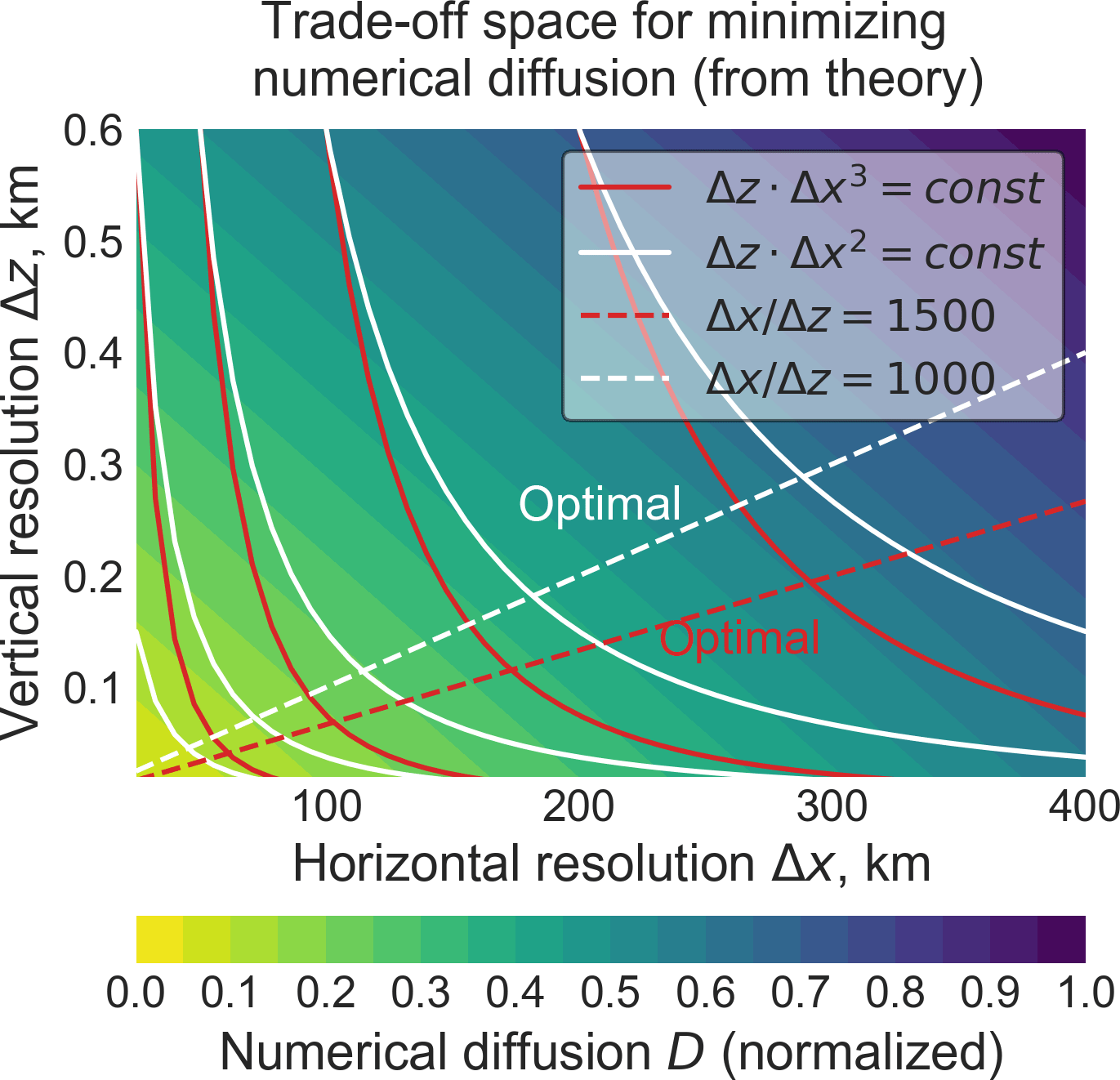
https://www.atmos-chem-phys.net/18/6039/2018/acp-18-6039-2018-f01

Figure 1Optimal combination of horizontal and vertical grid resolutions (Δx and Δz) for minimizing numerical diffusion of chemical plumes within a given amount of computational resources. Results are from the theoretical analysis of Sect. 2.3. The filled contours show the magnitude of the numerical diffusion term D from Eq. (23) as a function of Δx and Δz with $B / A = 500$ . The solid lines indicate a fixed amount of computational resources (P) in the trade-off between horizontal and vertical resolution, either using a fixed time step (ΔzΔx²=P) or accounting for the CFL condition (ΔzΔx³=P). The dashed lines from Eq. (27) indicate the corresponding optimal Δx ∕ Δz ratios to minimize numerical diffusion.

Download

3 Atmospheric plume simulation in the GFDL-FV3 dynamical core

We conduct an 8-day simulation of a chemically inert plume in the GFDL-FV3 (https://www.gfdl.noaa.gov/fv3/, “FV3” hereinafter) global 3-D dynamical core, with realistic sheared/stretched turbulent flow generated through a baroclinic instability test. FV3 uses the cubed-sphere geometry of Putman and Lin (2007) and the vertically Lagrangian discretization of Lin (2004). It includes a capability for transporting inert chemicals (“tracers”). The horizontal tracer transport algorithm is a high-dimension extension of the third-order piecewise parabolic method (PPM) (Lin and Rood, 1996) but is formally second-order accurate due to operator splitting between the two dimensions (Ullrich et al., 2010). The cubed-sphere grid avoids the polar singularity in the regular latitude–longitude grid and therefore permits efficient global high-resolution simulations on massively parallel machines. An intuitive explanation of the cubed-sphere geometry and resolution notation can be found at http://acmg.seas.harvard.edu/geos/cubed_sphere.html. FV3 has been implemented as a dynamical core in many global models including the NASA Goddard Earth Observing System (GEOS-5), the NCAR Community Earth System Model (CESM), the NCEP Global Forecast System (GFS) and the high-performance version of GEOS-Chem (GCHP) (see https://www.gfdl.noaa.gov/fv3/fv3-applications/).

Numerical diffusion takes place in FV3 during Eulerian horizontal advection (due to finite differencing of the spatial derivatives) and during vertical remapping of the Lagrangian surfaces to the model grid (due to interpolation error). Vertical remapping can use a larger time step than horizontal advection, but the interpolation scheme can be very diffusive if monotonicity is required. Our own comparisons of the vertically Lagrangian scheme to a high-order Eulerian scheme show that they have similar vertical diffusion (Appendix B).

https://www.atmos-chem-phys.net/18/6039/2018/acp-18-6039-2018-f02

Figure 2Atmospheric flow generated by the FV3 dynamical core in a baroclinic instability test, 16 days after initialization of the test and 8 days after the release of the chemical plume. Shown are surface pressures, 700 hPa flow streamlines and Lyapunov exponents λ measuring the stretching of the flow. Panel (a) shows results from the lowest horizontal resolution (C48, ≈ 200 km) and (b) shows results from the highest horizontal resolution (C384, ≈ 25 km), both with 20 vertical levels (L20). Increasing vertical resolution has little effect on the dynamics, as discussed in the text.

Download

An effective way to emulate realistic turbulent atmospheric flows in a dynamical core is the baroclinic instability test, originally developed by Jablonowski and Williamson (2006) as a dynamical core benchmark and subsequently used in tracer transport simulations (Jablonowski et al., 2008; Ullrich et al., 2016). Baroclinic instability is the main mechanism for cyclogenesis in midlatitudes. Instability can be triggered by applying a small perturbation to an initial reference state in geostrophic and hydrostatic balance. Starting from the initial perturbation, the baroclinic wave typically becomes observable around model day 4 and generates strong cyclones by day 8 (Jablonowski and Williamson, 2006).

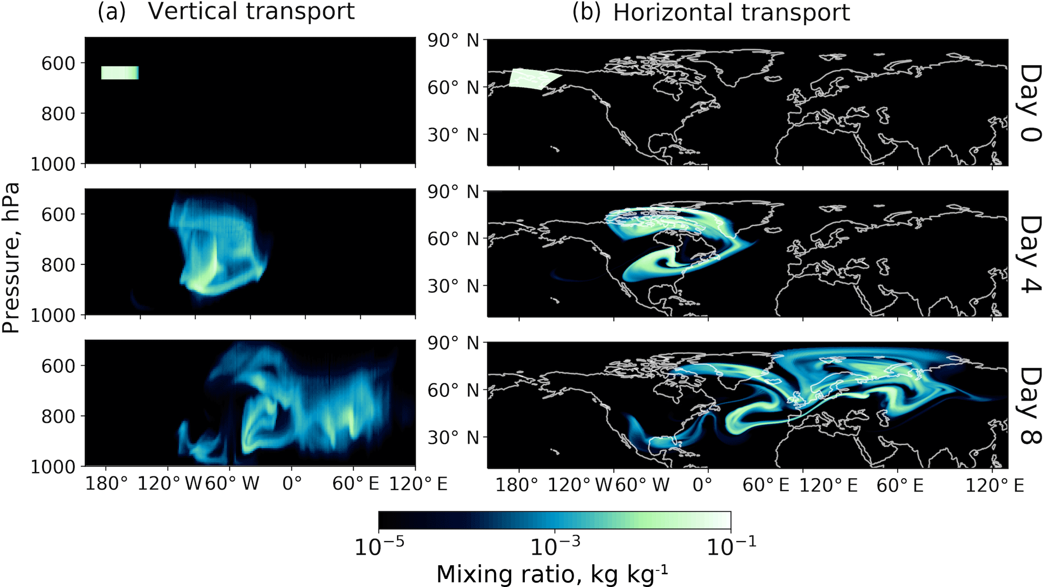
https://www.atmos-chem-phys.net/18/6039/2018/acp-18-6039-2018-f03

Figure 3The 8-day simulation of plume transport in the FV3 dynamical core at C384L160 resolution (≈ 25 km in horizontal and 6 hPa in vertical). The plume is initialized at 625 hPa over Alaska with a normalized mixing ratio of unity over a domain 1000 × 1000 km² in the horizontal and 50 hPa thickness in the vertical. Panel (a) shows the vertical and longitudinal transport of the plume as the meridionally averaged mixing ratio. Panel (b) shows the horizontal transport of the plume as column-averaged mixing ratios. Because mixing ratios are plotted here as meridional or vertical averages, the values are much lower than the actual values in the plume.

Download

https://www.atmos-chem-phys.net/18/6039/2018/acp-18-6039-2018-f04

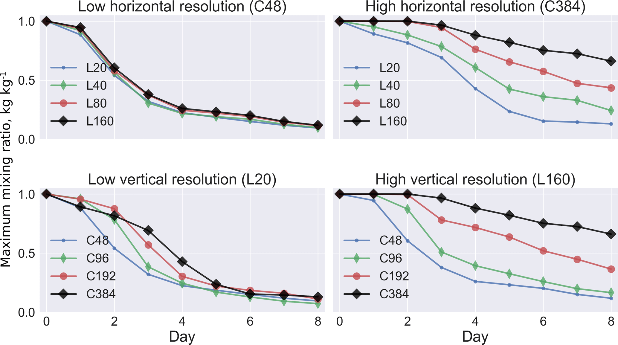
Figure 4Plume dilution due to numerical diffusion at different model grid resolutions. The plume is released in the free troposphere at northern midlatitudes with an initial mixing ratio of unity. Plume dilution is measured by the decrease in the maximum mixing ratio as a function of time. Model horizontal resolution is defined by a cubed-sphere grid ranging from C48 (≈ 200 km) to C384 (≈ 25 km). Vertical resolution is defined by an equally spaced isobaric grid ranging from L20 (20 levels, each 50 hPa thick) to L160 (160 levels, each 6 hPa thick).

Download

Here, we first run the baroclinic instability simulation for 8 days so that cyclones become intense enough for realistic flow shearing/stretching. We then initialize an inert tracer plume with uniform mixing ratio at the location where flow stretching is the strongest. This initial plume extends horizontally and vertically over a number of grid cells depending on the grid resolution, as detailed below. We continue the simulation for 8 days and diagnose the transport of the plume. Tracer transport involves solely advection. There is no subgrid turbulent diffusion or convection.

We conduct simulations at horizontal cubed-sphere resolutions ranging from C48 (≈ 200 km) to C384 (≈ 25 km) and vertical resolutions ranging from L20 (20 vertical layers) to L160. The vertical layers are equally spaced in pressure from the surface (1000 hPa in the reference state) to 1 hPa altitude. Thus, L20 has a vertical resolution of 50 hPa, corresponding to 0.6 km in the free troposphere at 600 hPa, which is roughly the vertical resolution of the GEOS-FP product used in the current version of GEOS-Chem. L160 has a vertical resolution of 6 hPa (roughly 80 m in the free troposphere), well beyond the resolution of any of the current global models. The same grid resolution is used for computing dynamics and tracer transport.

The time step for the Lagrangian remapping is 30 min for the lowest horizontal resolution case (C48) and is reduced proportionally at higher horizontal resolutions. Within this time step are eight sub-steps for horizontal dynamics calculations. The frequency of horizontal tracer advection calculations is determined on the fly based on the CFL criterion.

The plume is initialized with a uniform mixing ratio normalized to unity over a horizontal area corresponding to 6 × 6 C48 grid squares (roughly 1000 km × 1000 km) and vertically in a single layer in the L20 case (roughly 0.6 km thick) centered at 625 hPa (4 km) altitude. Thus, our coarsest simulation C48L20 resolves the initial plume with 6 × 6 × 1 grid cells, while our finest simulation C384L160 resolves it with 48 × 48 × 8 grid cells. The initialization is intended to describe a pollution plume once it has been lifted to the free troposphere and undergone fast initial horizontal fanning (Andreae et al., 1988; Heald et al., 2003). CTMs are generally successful at simulating this initial fanning but then fail to preserve the plume's coherent structure during the subsequent intercontinental transport (Heald et al., 2006; Zhang et al., 2008). The sensitivity of our results to the initial plume size will be discussed in Sect. 4.3.

4 Results and discussion

4.1 Plume transport and stretching

Figure 2 shows the surface pressures and 700 hPa wind fields on day 8 of the plume simulation, at C48L20 and C384L20 resolutions. The simulation describes a typical quasi-geostrophic system at midlatitudes with low and high pressure centers and the associated geostrophic winds. We find that increasing the horizontal resolution intensifies the cyclones, as shown in previous studies (Jablonowski and Williamson, 2006; Lauritzen et al., 2010), while increasing vertical resolution from L20 to L160 has almost no effect. Hence, the GCM emphasis on increasing horizontal resolution.

Also shown in Fig. 2 is the local Lyapunov exponent λ of the wind field. λ is the rate constant at which nearby air parcels separate in the direction of the flow, i.e., the intensity of flow stretching. Rastigejev et al. (2010) showed theoretically that the Lyapunov exponent should be a predictor of numerical diffusion in Eulerian models, and Eastham and Jacob (2017) confirmed this in GEOS-Chem model simulations. We calculate the Lyapunov exponent locally, using the formula derived by Eastham and Jacob (2017):

\begin{matrix} (28) & λ \approx \frac{|Δ u| + |Δ v|}{Δ x + Δ y}, \end{matrix}

where Δu and Δv are the changes in wind speed between the local grid cell and the grid cell downwind, and Δx and Δy are the corresponding grid spacings. Between 30^∘ N and 60^∘ N where the plume transport takes place, the Lyapunov exponents are of order 10⁻⁵ s⁻¹, consistent with values derived from the GEOS-FP wind data (Eastham and Jacob, 2017). Higher horizontal resolution increases stretching because small-scale eddies are better resolved, which offsets some of the reduction in numerical diffusion (Rastigejev et al., 2010). We find the 700 hPa vertical wind speed w at 30–60^∘ N of −0.1 ± 1.0 cm s⁻¹ (mean ±1 SD), typical of the range of large-scale vertical wind speeds in the real atmosphere. Thus, the FV3 simulation provides a realistic environment to investigate how global-scale transport of chemical plumes is sensitive to model grid resolution. It does not account for deep convection or boundary layer turbulence, but our focus here is on the free troposphere under the prevailing stable conditions that allow for plume preservation during global-scale transport. The plume may originate from a convective updraft, and it may be eventually entrained and mixed in the turbulent boundary layer, but convection and boundary layer turbulence are out of scope.

Figure 3 illustrates the evolution of the plume over the 8-day period in the C384L160 case (≈ 25 km, 6 hPa resolution). The plume is initialized over Alaska, reaches eastern North America by day 4, and Eurasia by day 8, with strong filamentation along the way due to wind shear. Such rapid transport and filamentation are typical of free tropospheric plumes at northern midlatitudes (Stohl et al., 2002). The plume gradually subsides and dilutes vertically over the 8-day period, with a subsidence rate typical of observations (Crawford et al., 2004). The spreading and dilution of the plume apparent in Fig. 3 are due in part to the plotting of column and meridional average mixing ratios for visualization purposes; the actual numerical diffusion is less and can be quantified by the mixing ratio decay and entropy increase for the actual plume, as described in Sect. 4.2.

4.2 Numerical diffusion at different grid resolutions

Exact solution to the advection equation conserves the mixing ratio, even for divergent or sheared flow (Chapter 7.2 of Brasseur and Jacob, 2017). Our simulation includes advection as the only process. It follows that any mixing ratio decay in the model plume must be due solely to numerical diffusion and provides a metric for this diffusion.

Figure 4 shows the rate of decay of the maximum mixing ratio in the plume for the different horizontal and vertical resolutions of our simulations. The timescale for this decay diagnoses the rate of plume dissipation from numerical diffusion and can be used to compare different grid resolutions (Rastigejev et al., 2010; Eastham and Jacob, 2017).

At the lowest resolution (C48L20), the maximum mixing ratio in the plume drops from 1.0 to 0.1 after 8 days. Such rapid diffusion is consistent with the midlatitude results of Eastham and Jacob (2017) using GEOS-FP winds. Starting from C48L20, solely increasing the vertical resolution has no benefit in reducing numerical diffusion (Fig. 4, top left panel). Solely increasing horizontal resolution has some benefit for the first 4 days of aging, but by day 5 the benefit is gone (Fig. 4, bottom left panel). This is consistent with the theory in Sect. 2.1 that inadequate resolution in one direction will limit the overall accuracy, making grid refinement in the other direction useless.

However, once the resolution of one dimension is high enough that it is no longer a limiting factor, grid refinement in the other direction becomes effective. This is illustrated in the right panels of Fig. 4. Increasing vertical resolution in a C384 simulation has sustained benefit from L20 to L160, and increasing horizontal resolution in a L160 simulation has sustained benefit from C48 to C384. At the highest resolution (C384L160), the decay in the maximum mixing ratio is only 35 % after 8 days of transport, a drastic improvement over the simulation cases presented by Rastigejev et al. (2010) and Eastham and Jacob (2017).

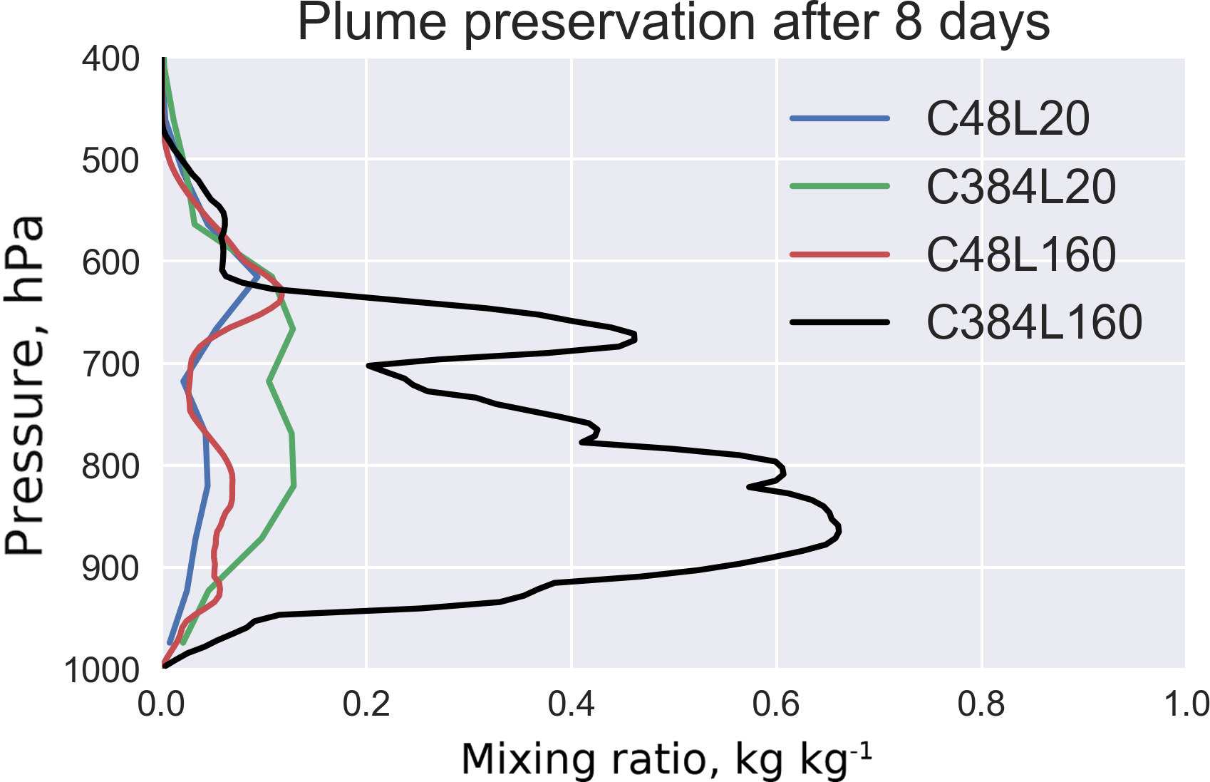
https://www.atmos-chem-phys.net/18/6039/2018/acp-18-6039-2018-f05

Figure 5Vertical profile of the maximum mixing ratio for each model vertical level after 8 days of simulation, at low model resolution (C48L20), high model resolution (C384L160) and intermediate cases where only horizontal resolution or vertical resolution is increased from the low-resolution case (C384L20, C48L160).

Download

https://www.atmos-chem-phys.net/18/6039/2018/acp-18-6039-2018-f06

Figure 6Same as Fig. 4 but with entropy instead of maximum mixing ratio as a diagnostic for numerical diffusion. The entropy is initialized on day 0 with a value of 1. Pure advection conserves entropy but diffusion increases it.

Download

The behavior of decay rates in Fig. 4 lends further insights into numerical diffusion. We see that the decay rates are initially slow and then abruptly increase. This is because the plume is initially well resolved on the grid, but as the plume gradually filaments and becomes poorly resolved, fast numerical diffusion takes over. Increasing horizontal resolution delays the onset of this fast numerical diffusion, as seen most dramatically in the bottom left panel of Fig. 4. Thus, a factor in the choice of resolution should be the extent of time over which the model plumes must be preserved, considering that molecular diffusion will eventually dissipate the plumes in the actual atmosphere as they filament down to the millimeter Kolmogorov scale (Chapter 8 of Brasseur and Jacob, 2017). Observations show that intercontinental free tropospheric plumes can retain their structure for at least a week (Heald et al., 2003; Zhang et al., 2008), so there is benefit in the highest range of resolutions investigated in our simulations.

Figure 5 shows the vertical profile of maximum mixing ratios for each model level after 8 days of simulation, at the lowest model resolution (C48L20), the highest model resolution (C384L160) and intermediate cases where only horizontal or vertical resolution is increased from the low-resolution case (C384L20, C48L160). Starting from C48L20, solely increasing either the horizontal resolution (to C384L20) or the vertical resolution (to C48L160) has limited improvement on the vertical profile. This is the familiar picture of models being unable to preserve the vertical structure of pollution plumes on intercontinental scales (Heald et al., 2003). Increasing both horizontal and vertical resolutions (to C384L160) drastically improves the preservation of the vertical profile and largely fixes the problem. The surface concentrations are close to zero in all cases but this is because the FV3 dynamical core does not include boundary layer physics. From the concentrations at 900–950 hPa, we can conclude that the high-resolution simulation when implemented in a full GCM would lead to much stronger localized impact of the subsiding plume on surface concentrations.

Maximum mixing ratio in the plume is an extreme value diagnostic that is relevant for plume observation and impact but is an imperfect measure of plume dilution (Eastham and Jacob, 2017). As shown in Fig. 3, the plume shears into multiple filaments as it ages but the maximum mixing ratio diagnoses just one of these filaments. Also, numerical diffusion will first erode the plume as its edges while preserving the maximum mixing ratio at the center. Eastham and Jacob (2017) used the expanding size of the plume as an alternate diagnostic but this relies on an arbitrary concentration threshold.

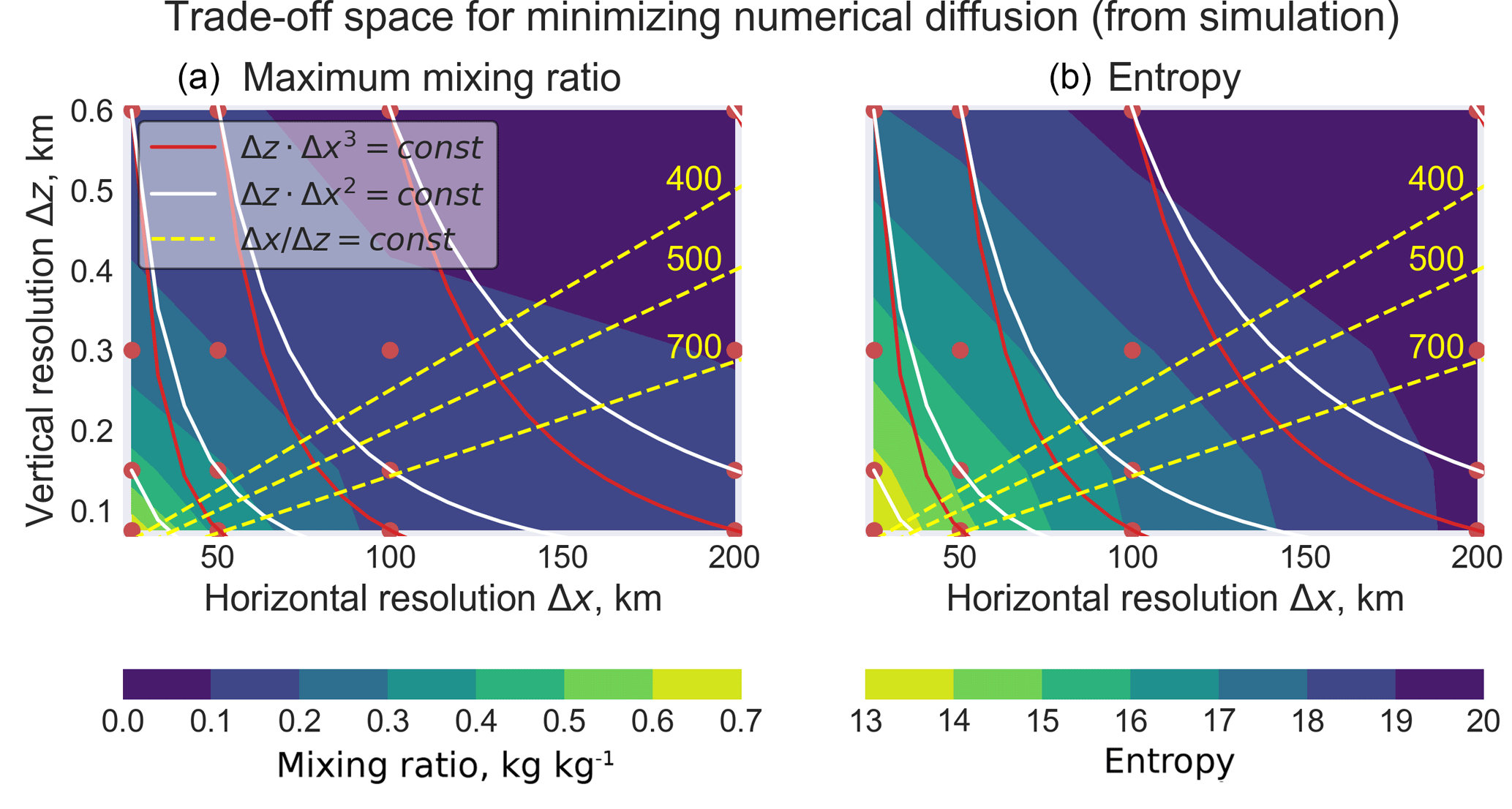
https://www.atmos-chem-phys.net/18/6039/2018/acp-18-6039-2018-f07

Figure 7Optimal combination of horizontal and vertical grid resolutions (Δx and Δz) for minimizing numerical diffusion of chemical plumes within a given amount of computational resources. Results are from the FV3 simulation (data from Figs. 4 and 6) and can be compared to Fig. 1 that shows similar results from theoretical analysis. The filled contours show the maximum plume mixing ratio (a) or entropy (b) on day 8 of the simulations as metrics of numerical diffusion. High maximum mixing ratio and low entropy are indicative of low numerical diffusion. The red dots are the data points used to construct the contours, with each point corresponding to a simulation at a given resolution. The solid lines indicate a fixed amount of computational resources (P) in the trade-off between horizontal and vertical resolution, either using a fixed time step (ΔzΔx²=P) or accounting for the CFL condition (ΔzΔx³=P). The yellow dashed lines show different Δx ∕ Δz ratios (400, 500, 700).

Download

As a more general diagnostic of plume preservation, we calculate the entropy that takes into account all grid cells in the global domain (Lauritzen and Thuburn, 2012). The entropy S of a 3-D mixing ratio field can be calculated by

\begin{matrix} (29) & S = - k \sum_{i = 1}^{n} m_{i} C_{i} \log C_{i}, \end{matrix}

where n is the total number of grid cells of index i, C_i is the mixing ratio, m_i is the mass of air in the grid cell, and k is a scaling factor such that the initial entropy is unity. Pure advection conserves entropy but diffusion increases it, and S is maximized when the mixing ratio field C becomes uniform (complete mixing). A non-monotonic advection scheme can unphysically decrease entropy, but here we use strictly monotonic schemes in both horizontal and vertical dimensions so this would not happen. Entropy would increase in a real-world plume as filamentation leads to eventual plume dissipation by molecular diffusion, but numerical diffusion is much faster on our scales of relevance (D'Isidoro et al., 2010). Thus, our goal here is to minimize entropy, i.e., minimize numerical diffusion.

Figure 6 shows the increase in entropy as the plume dilutes at different model grid resolutions. Results are similar to the maximum mixing ratio diagnostic (Fig. 4) in showing the limiting effects of either horizontal or vertical resolution, and the benefit of coupling the two to improve the simulation. One difference is the absence of a time lag for plume dilution. Whereas the maximum mixing ratio is initially sheltered from numerical diffusion if the plume is resolved by a number of grid cells, numerical diffusion erodes the plume edges and the thinner filaments, and this is captured by the entropy diagnostic. The entropy diagnostic also shows a slowdown of plume dilution with time, particularly at coarse resolution, and this is due to the smoothing of the plume that allows concentration gradients to be better represented by the numerical schemes. Nevertheless, the entropy continues to increase even as plume edges become smoother. Ultimately, the choice of maximum mixing ratio or entropy as a diagnostic of plume dissipation may depend on the application, but the implied requirements for grid resolution are similar. This is discussed further below (Sect. 4.3).

4.3 Optimal combination of horizontal and vertical grid resolution

The results from Sect. 4.2, following on the theoretical analysis of Sect. 2, show that preserving plumes in global models may be limited by either horizontal or vertical resolution. It follows that there must be an optimal ratio of horizontal to vertical grid spacing (Δx ∕ Δz)_opt for simulating the global-scale transport of plumes, as there is for the dynamical criteria reviewed in the introduction. We derived such a ratio from theoretical analysis in Sect. 2, and here we derive it from the FV3 plume simulations.

Figure 7 illustrates the trade-offs between horizontal and vertical resolution in the FV3 plume simulations, presented in a similar manner to the results of the theoretical analysis in Fig. 1. The contours measure the preservation of the plume after 8 days, as diagnosed by either the maximum mixing ratio or the entropy, using the day 8 data from Figs. 4 and 6 with additional simulations at intermediate resolutions to better define the contours. As in Sect. 2.3, we aim to preserve the maximum mixing ratio and/or minimize entropy under the computational trade-offs ΔzΔx³=P and ΔzΔx²=P. The actual computational costs of our GFDL-FV3 simulations follow the ΔzΔx³=P curve, since the time step is reduced proportionally with the horizontal resolution. The solid lines show the computational trade-offs. Along each trade-off line, it is generally beneficial to move away from Δx ∕ Δz < 100 (the upper left region of Fig. 7, Δx=25–50 km, Δz=0.6 km) and toward Δx ∕ Δz ∼ 1000 (the bottom region of Fig. 7, Δx=50–200 km, Δz=0.08 km), since it leads to better preservation of the plume without incurring more computational cost. Thus, we already see that the current generation of models (Δx ∕ Δz ∼ 20) is out of balance in privileging horizontal over vertical resolution.

As in Sect. 2.3, the optimal ratio (Δx ∕ Δz)_opt is defined by the point where the computational trade-off line parallels the contour line. Different ratios Δx ∕ Δz are shown as yellow dashed lines in Fig. 7. For the ΔzΔx³=P trade-off (the red solid lines in Fig. 7), the optimal Δx ∕ Δz is in the range 400–700. For the ΔzΔx²=P trade-off (white solid lines), the optimal Δx ∕ Δz is around 400. This is consistent with the theoretical derivation in Sect. 2.3 where the optimal Δx ∕ Δz is of order 1000.

We conducted sensitivity tests with plumes of different initial vertical thicknesses and horizontal extents, and found similar results. Thicker plumes have better initial preservation of the maximum mixing ratio but this advantage is rapidly lost as the plume filaments. Although the theoretical analysis of Sect. 2 implies that (Δx ∕ Δz)_opt should depend on the plume size, this applies to the stretched rather than to the initial plume. During model transport, plumes of different initial thicknesses tend to be stretched to similar steady-state thicknesses where the stretching rate (thinning the plume) is balanced by the numerical diffusion rate (thickening the plume) (Rastigejev et al., 2010).

The estimated (Δx ∕ Δz)_opt should not greatly depend on the advection scheme used, since fast numerical diffusion occurs when the plume has filamented to the point where gradients cannot be resolved and any advection scheme collapses to first-order accurate. One concern is whether FV3 represents realistically the ratio of vertical-to-horizontal shear that would occur in a wet atmosphere; this should be tested in simulations in an actual GCM. Nevertheless, it appears that the vertical resolution requirements for global simulation of chemical plumes are larger than the ratio (Δx ∕ Δz)_opt ∼ 100 derived from dynamical concerns of resolving fronts and gravity waves, and that current models have inadequate vertical resolutions.

Our recommendation to increase vertical resolution in the free troposphere is specific to global models, and our emphasis on an optimal Δx ∕ Δz is to make the point that the simulation of global-scale plumes with large horizontal/vertical aspect ratios (reflecting the strong horizontal wind shear and vertically stable conditions of the free troposphere) is currently limited by vertical rather than by horizontal model resolution. The situation would be very different in cloud-resolving models (Δx < 1 km) where turbulence is much more isotropic.

5 Conclusions and implications for global modeling of chemical plumes

Current global models are unable to simulate the observed persistence of chemical plumes in the free troposphere on intercontinental scales. The plumes dilute too rapidly due to numerical diffusion in sheared flow. This is a major problem for global simulations of atmospheric composition and for diagnosing intercontinental pollution influences on surface air quality. We investigated how this problem could be solved through increasing horizontal and vertical grid resolutions, and in what optimal combination. We used for this purpose the GFDL-FV3 global dynamical core to perform plume transport simulations, driven by flow with realistic shear as generated from a baroclinic instability test. The flexibility of this dynamical core allowed us to conduct simulations over cubed-sphere horizontal resolutions ranging from C48 (≈ 200 km) to C384 (≈ 25 km) and vertical resolutions ranging from L20 (50 hPa) to L160 (6 hPa).

We began with a theoretical analysis of the plume advection problem to show that numerical diffusion may be limited by either horizontal grid resolution (Δx) or vertical resolution (Δz). This analysis must take into account that increasing horizontal resolution is more costly than increasing vertical resolution, as expressed by Δx^kΔz=P where P denotes the amount of computational resources available and k=2 (fixed time step) or k=3 (time step adjusted for the CFL condition). We derived from this analysis an optimal ratio (Δx ∕ $Δ z)_{opt} \approx k (w / 2 u) (L / H)^{2} \sim 1000$ for resolving the long-range transport of plumes, where u and w are the horizontal and vertical components of the wind, and L and H are the horizontal and vertical dimensions of the plume. This is larger than the optimal ratio (Δx ∕ Δz)_opt ∼ 100 derived from dynamical considerations of resolving fronts and gravity waves. Current global atmospheric models have Δx ∕ Δz∼20 in the free troposphere (Δx ∼ 10 km, Δz ∼ 0.5 km), with an emphasis on continued improvement in horizontal resolution to the neglect of vertical resolution. This explains why excessively fast dilution of chemical plumes takes place in these models. The problem would not apply in the boundary layer, where plumes are more isotropic (much lower L∕H) and models have larger Δx ∕ Δz ratios. But global-scale plume transport takes place mainly in the free troposphere.

We applied the FV3 dynamical core to simulate the transport over 8 days of a chemically inert free tropospheric plume at northern midlatitudes. Transport in the dynamical core is solely by advection, and exact solution should therefore preserve the initial mixing ratio in the plume. We diagnosed numerical diffusion over the 8-day simulation by the decay of the maximum mixing ratio and the increase in entropy. We demonstrated how improvements in preserving the plume during transport can be limited by either horizontal or vertical resolution, in a manner consistent with the theoretical analysis. Our highest-resolution simulation (C384L160) preserved the maximum mixing ratio in the plume to within 35 % after 8 days in strongly sheared flow, retained the vertical structure of the plume and led to much larger local intercontinental impacts on surface air than the coarser-resolution simulations. The required vertical resolution in the free troposphere is 6 hPa (≈ 80 m), considerably finer than in current global models.

There are strong reasons for GCMs to focus on increasing horizontal resolution, as this allows better representation of cyclogenesis and other aspects of the meteorological simulation. However, simulations of global chemical transport require higher vertical resolution in the free troposphere. Considering that the free troposphere accounts for only about a third of all vertical levels in the current generation of models, adding vertical resolution only to that part of the atmosphere would not be expensive. A proper vertical resolution in the free troposphere would also benefit the simulation of water vapor with implications for the radiative budget and for cloud formation. Within the framework of current GCMs, it may be possible to improve chemical transport by conducting offline CTM simulations with high vertical resolution, interpolating the meteorological archive from the parent GCM. The feasibility of such hybrid-resolution simulations has been studied by Methven and Hoskins (1999). Adaptive mesh refinement (AMR) is also a computationally efficient approach to improve plume simulations (Semakin and Rastigejev, 2016), but implementing AMR in existing CTMs requires significant engineering efforts especially on parallelization.

Code availability

The FV3 source code was obtained from https://www.gfdl.noaa.gov/cubed-sphere-quickstart/. All scripts for model configuration and data analysis are available at https://github.com/JiaweiZhuang/FV3_util (https://doi.org/10.5281/zenodo.1214605). A Python package named “cubedsphere” (https://github.com/JiaweiZhuang/cubedsphere, https://doi.org/10.5281/zenodo.1095677) was developed by the lead author for analyzing data on the cubed-sphere grid. We use xarray (Hoyer and Hamman, 2017) to process NetCDF data that are larger than computer memory.

Relating

\partial^{2} C / \partial t^{2}

and

\partial^{2} C / \partial x^{2}

through the advection equation

Following Odman (1997), we start with the 1-D advection equation:

\begin{matrix} (A1) & \frac{\partial C}{\partial t} + u \frac{\partial C}{\partial x} = 0 . \end{matrix}

The equation is solved by the 1-D upwind scheme:

\begin{matrix} (A2) & \frac{C (n + 1, i) - C (n, i)}{Δ t} + u \frac{C (n, i) - C (n, i - 1)}{Δ x} = 0 . \end{matrix}

Using the modified equation approach introduced in Sect. 2, we find the numerical scheme better represents the equation

\begin{matrix} (A3) & \frac{\partial C}{\partial t} + u \frac{\partial C}{\partial x} = - \frac{Δ t}{2} \frac{\partial^{2} C}{\partial t^{2}} + \frac{u Δ x}{2} \frac{\partial^{2} C}{\partial x^{2}} + o (Δ t + Δ x) . \end{matrix}

We apply the operation $(Δ t / 2) (\partial / \partial t)$ to Eq. (A3):

\begin{array}{l} \frac{Δ t}{2} \frac{\partial}{\partial t} [\frac{\partial C}{\partial t} + u \frac{\partial C}{\partial x}] = \frac{Δ t}{2} \frac{\partial}{\partial t} [- \frac{Δ t}{2} \frac{\partial^{2} C}{\partial t^{2}} \\ (A4) & + \frac{u Δ x}{2} \frac{\partial^{2} C}{\partial x^{2}} + o (Δ t + Δ x)] . \end{array}

The right-hand side of Eq. (A4) only contains high-order terms such as Δt² and ΔtΔx, so it can be simply written as o(Δt+Δx):

\begin{matrix} (A5) & \frac{Δ t}{2} \frac{\partial^{2} C}{\partial t^{2}} + \frac{u Δ t}{2} \frac{\partial^{2} C}{\partial t \partial x} = o (Δ t + Δ x) . \end{matrix}

We subtract Eq. (A5) from Eq. (A3) to cancel the (Δt∕2)(∂²C ∕ ∂t²) term:

\begin{matrix} (A6) & \frac{\partial C}{\partial t} + u \frac{\partial C}{\partial x} = \frac{u Δ t}{2} \frac{\partial^{2} C}{\partial t \partial x} + \frac{u Δ x}{2} \frac{\partial^{2} C}{\partial x^{2}} + o (Δ t + Δ x) . \end{matrix}

Compared to Eq. (A3), the second-order time derivative ( $- Δ t / 2$ )(∂²C ∕ ∂t²) is now replaced by the mixed derivative (uΔt∕2)(∂²C ∕ $\partial t \partial x$ ).

To further eliminate this mixed derivative, we apply the operation (uΔt∕2)(∂ ∕ ∂x) to Eq. (A6)

\begin{array}{l} \frac{u Δ t}{2} \frac{\partial}{\partial x} [\frac{\partial C}{\partial t} + u \frac{\partial C}{\partial x}] = \frac{u Δ t}{2} \frac{\partial}{\partial x} \\ (A7) & [- \frac{Δ t}{2} \frac{\partial^{2} C}{\partial t^{2}} + \frac{u Δ x}{2} \frac{\partial^{2} C}{\partial x^{2}} + o (Δ t + Δ x)] . \end{array}

Again, the right-hand side of Eq. (A7) can be simply written as o(Δt+Δx):

\begin{matrix} (A8) & \frac{u Δ t}{2} \frac{\partial^{2} C}{\partial x \partial t} + \frac{u^{2} Δ t}{2} \frac{\partial^{2} C}{\partial x^{2}} = o (Δ t + Δ x) . \end{matrix}

We add Eq. (A8) to Eq. (A6) to cancel the (uΔt∕2)(∂²C ∕ $\partial x \partial t$ ) term:

\begin{array}{l} \frac{\partial C}{\partial t} + u \frac{\partial C}{\partial x} = - \frac{u^{2} Δ t}{2} \frac{\partial^{2} C}{\partial x^{2}} + \frac{u Δ x}{2} \frac{\partial^{2} C}{\partial x^{2}} \\ (A9) & + o (Δ t + Δ x) . \end{array}

Now, all time derivatives except the original ∂C ∕ ∂t are removed. The time step Δt can also be removed by introducing the CFL number $α = u Δ t / Δ x$ . The first term on the right-hand side of Eq. (A9) becomes

\begin{matrix} (A10) & - \frac{u^{2} Δ t}{2} \frac{\partial^{2} C}{\partial x^{2}} = - α \frac{u Δ x}{2} \frac{\partial^{2} C}{\partial x^{2}} . \end{matrix}

Thus, Eq. (A9) can be further simplified to

\begin{matrix} (A11) & \frac{\partial C}{\partial t} + u \frac{\partial C}{\partial x} = (1 - α) \frac{u Δ x}{2} \frac{\partial^{2} C}{\partial x^{2}} + o (Δ t + Δ x) . \end{matrix}

Comparing Eq. (A11) to Eq. (A3), the time derivative (Δt∕2)(∂²C ∕ ∂t²) is approximated by the spatial derivative (αuΔx∕2)(∂²C ∕ ∂x²). This means that, as long as the CFL condition is satisfied, the time discretization error will not limit the overall accuracy. This conclusion still applies to a 3-D advection equation, although the above mathematical derivation will produce mixed derivatives like ∂²C ∕ $\partial x \partial y$ , so a compact formula like Eq. (A11) cannot be easily obtained.

Appendix B: Comparing vertical numerical diffusion in FV3 and TPCORE schemes

Here, we use the GEOS-Chem CTM to compare vertical numerical diffusion in FV3's advection scheme to that in TPCORE, a 3-D Eulerian advection scheme (Lin and Rood, 1996). TPCORE is the standard advection scheme in the “classic” version of the GEOS-Chem CTM (Bey et al., 2001), while FV3 is used in the high-performance version of GEOS-Chem (GCHP; Long et al., 2017; Yu et al., 2018). Unlike FV3, TPCORE uses a regular latitude–longitude geometry and a vertically Eulerian discretization. When the CFL number is less than 1, the horizontal tracer transport uses the monotonic PPM as in FV3; otherwise, a semi-Lagrangian method is used. The vertical tracer transport uses PPM with Huynh's second constraint (Huynh, 1997). We use a C48 horizontal resolution for GEOS-Chem with FV3 and a corresponding 2^∘ × 2.5^∘ resolution for GEOS-Chem with TPCORE. Both versions use the native GEOS-FP 72-level hybrid sigma-pressure vertical coordinate and a time step of 15 min.

https://www.atmos-chem-phys.net/18/6039/2018/acp-18-6039-2018-f08

Figure B1Comparing vertical diffusion in the GEOS-Chem CTM using either the TPCORE Eulerian advection scheme (b–d) or the FV3 vertically Lagrangian advection scheme (e–g). A Hadley-like circulation test is applied to both schemes with rising motion in the first 12 h followed by return to the original state in the next 12 h (Kent et al., 2014). The tracer field is independent of longitude. The true solution at the final state (t=24 h) should be the same as the initial condition (a), and the deviation from the initial condition is due to numerical error. The error (d, g) is defined as final state minus initial state.

Download

We use the idealized Hadley-like circulation test in the 2012 Dynamical Core Model Intercomparison Project (Kent et al., 2014) to benchmark the vertical diffusion in both models. The simulation is illustrated in Fig. B1. The initial tracer layer (Fig. B1, left panel) is advected in the vertical by a Hadley-like flow (Fig. B1, middle panels) and then gets reverted to the original state by a reverse flow (Fig. B1, right panels). The true solution at the final state should be the same as the initial condition, and the deviation from the initial condition is due to numerical error. The error norm can be calculated by

\begin{matrix} (B1) & l = \frac{\sum_{i = 1}^{n} m_{i} |C_{i} - C_{i, t r u e}|}{\sum_{i = 1}^{n} m_{i} |C_{i, t r u e}|}, \end{matrix}

where n is the total number of grid cells of index i, m_i is the mass of air in the grid cell, C_i is the mixing ratio at the final state, and C_i,true is the mixing ratio at the initial state. We find l=19.0 % for TPCORE and l=16.2 % for FV3, indicating that the vertically Lagrangian scheme in FV3 has a diffusion similar to the Eulerian scheme in TPCORE.

There are many equivalences between remapping schemes and advection schemes. For example, both higher-order remapping and higher-order advection schemes are not monotonic by default and need additional limiters or constraints to prevent overshoots. If gradients are sharp, monotonic limiters will degrade higher-order schemes to first order, at the expense of making the schemes more diffusive. Increasing the grid resolution will make both remapping and advection schemes more accurate and less diffusive. Due to these similarities between advection and remapping, our Eulerian-based theoretical analysis in Sect. 2 should also apply to vertically Lagrangian schemes.

Supplement

The supplement related to this article is available online at: https://doi.org/10.5194/acp-18-6039-2018-supplement.

Competing interests

The authors declare that they have no conflict of interest.

Acknowledgements

The authors would like to thank Lucas Harris, Xi Chen and Shian-Jiann Lin at GFDL for general guidance on the GFDL-FV3 model. Resources supporting this work were provided by the NASA High-End Computing (HEC) Program through the NASA Advanced Supercomputing (NAS) Division at Ames Research Center. This work was supported by the NASA Modeling, Analysis, and Prediction (MAP) Program.Edited by: Anja Schmidt
Reviewed by: three anonymous referees

References

Andreae, M. O., Browell, E. V., Garstang, M., Gregory, G. L., Harriss, R. C., Hill, G. F., Jacob, D. J., Pereira, M. C., Sachse, G. W., Setzer, a. W., Dias, P. L. S., Talbot, R. W., Torres, A. L., and Wofsy, S. C.: Biomass-burning emissions and associated haze layers over Amazonia, J. Geophys. Res., 93, 1509–1527, https://doi.org/10.1029/JD093iD02p01509, 1988.

Balaji, V.: Climate Computing: The State of Play, Comput. Sci. Eng., 17, 9–13, https://doi.org/10.1109/MCSE.2015.109, 2015.

Bey, I., Jacob, D. J., Yantosca, R. M., Logan, J. A., Field, B. D., Fiore, A. M., Li, Q., Liu, H. Y., Mickley, L. J., and Schultz, M. G.: Global modeling of tropospheric chemistry with assimilated meteorology: Model description and evaluation, J. Geophys. Res.-Atmos., 106, 23073–23095, 2001.

Brasseur, G. P. and Jacob, D. J.: Modeling of Atmospheric Chemistry, Cambridge University Press, Cambridge, 2017.

Crawford, J. H., Heald, C. L., Fuelberg, H. E., Morse, D. M., Sachse, G. W., Emmons, L. K., Gille, J. C., Edward, D. P., Deeter, M. N., Chen, G., Olson, J. R., Connors, V. S., Kittaka, C., and Hamlin, A. J.: Relationship between measurements of pollution in the Troposphere (MOPITT) and in situ observations of CO based on a large-scale feature sampled during TRACE-P, J. Geophys. Res.-Atmos., 109, 1–10, https://doi.org/10.1029/2003JD004308, 2004.

D'Isidoro, M., Maurizi, A., and Tampieri, F.: Effects of resolution on the relative importance of numerical and physical horizontal diffusion in atmospheric composition modelling, Atmos. Chem. Phys., 10, 6213, https://doi.org/10.5194/acp-10-6213-2010, 2010.

Dritschel, D. G. and McKiver, W. J.: Effect of Prandtl's ratio on balance in geophysical turbulence, J. Fluid Mech., 777, 569–590, https://doi.org/10.1017/jfm.2015.348, 2015.

Durran, D. R.: Numerical Methods for Fluid Dynamics: With Applications to Geophysics, https://doi.org/10.1007/978-1-4419-6412-0, 2010.

Eastham, S. D. and Jacob, D. J.: Limits on the ability of global Eulerian models to resolve intercontinental transport of chemical plumes, Atmos. Chem. Phys., 17, 2543–2553, https://doi.org/10.5194/acp-17-2543-2017, 2017.

Geophysical Fluid Dynamics Laboratory (GFDL): Quickstart Guide: Idealized finite-volume model https://www.gfdl.noaa.gov/cubed-sphere-quickstart/, last access: April 2018.

Goldstein, A. H., Millet, D. B., McKay, M., Jaeglé, L., Horowitz, L., Cooper, O., Hudman, R., Jacob, D. J., Oltmans, S., and Clarke, A.: Impact of Asian emissions on observations at Trinidad Head, California, during ITCT 2K2, J. Geophys. Res.-Atmos., 109, 1–13, https://doi.org/10.1029/2003JD004406, 2004.

Haarsma, R. J., Roberts, M. J., Vidale, P. L., Catherine, A., Bellucci, A., Bao, Q., Chang, P., Corti, S., Fučkar, N. S., Guemas, V., Von Hardenberg, J., Hazeleger, W., Kodama, C., Koenigk, T., Leung, L. R., Lu, J., Luo, J. J., Mao, J., Mizielinski, M. S., Mizuta, R., Nobre, P., Satoh, M., Scoccimarro, E., Semmler, T., Small, J., and Von Storch, J. S.: High Resolution Model Intercomparison Project (HighResMIP v1.0) for CMIP6, Geosci. Model Dev., 9, 4185–4208, https://doi.org/10.5194/gmd-9-4185-2016, 2016.

Haiden, T., Janousek, M., Bidlot, J., Ferranti, L., Prates, F., Vitart, F., Bauer, P., and Richardson, D. S.: Evaluation of ECMWF forecasts, including the 2016 resolution upgrade, ECMWF Tech. Memo., 792(January 2017) [online] Available from: http://www.ecmwf.int/sites/default/files/elibrary/2015/15275-evaluation-ecmwf-forecasts-including-2014-2015-upgrades.pdf, 2016.

Heald, C. L., Jacob, D. J., Fiore, A. M., Emmons, L. K., Gille, J. C., Deeter, M. N., Warner, J., Edwards, D. P., Crawford, J. H., Hamlin, A. J., Sachse, G. W., Browell, E. V., Avery, M. A., Vay, S. A., Westberg, D. J., Blake, D. R., Singh, H. B., Sandholm, S. T., Talbot, R. W., and Fuelberg, H. E.: Asian outflow and trans-Pacific transport of carbon monoxide and ozone pollution: An integrated satellite, aircraft, and model perspective, J. Geophys. Res.-Atmos., 108, 4804, https://doi.org/10.1029/2003JD003507, 2003.

Heald, C. L., Jacob, D. J., Park, R. J., Alexander, B., Fairlie, T. D., Yantosca, R. M., and Chu, D. A.: Transpacific transport of Asian anthropogenic aerosols and its impact on surface air quality in the United States, J. Geophys. Res.-Atmos., 111, D14310, https://doi.org/10.1029/2005JD006847, 2006.

Holton, J. R.: An Introduction to Dynamic Meteorology, Elsevier, 2004.

Hoyer, S. and Hamman, J. J.: xarray: N-D labeled Arrays and Datasets in Python, J. Open Res. Softw., 5, 1–6, https://doi.org/10.5334/jors.148, 2017.

Hudman, R. C., Jacob, D. J., Cooper, O. R., Evans, M. J., Heald, C. L., Park, R. J., Fehsenfeld, F., Flocke, F., Holloway, J., Hübler, G., Kita, K., Koike, M., Kondo, Y., Neuman, A., Nowak, J., Oltmans, S., Parrish, D., Roberts, J. M., and Ryerson, T.: Ozone production in transpacific Asian pollution plumes and implications for ozone air quality in California, J. Geophys. Res. D Atmos., 109, 1–14, https://doi.org/10.1029/2004JD004974, 2004.

Huynh, H. T.: Schemes and constraints for advection, in: Fifteenth International Conference on Numerical Methods in Fluid Dynamics, 498–503, Springer, Berlin, 1997.

Ingram, W. J.: On the robustness of the water vapor feedback: GCM vertical resolution and formulation, J. Clim., 15, 917–921, https://doi.org/10.1175/1520-0442(2002)015<0917:OTROTW>2.0.CO;2, 2002.

Jablonowski, C. and Williamson, D. L.: A baroclinic instability test case for atmospheric model dynamical cores, Q. J. Roy. Meteor. Soc., 132, 2943–2975, https://doi.org/10.1256/qj.06.12, 2006.

Jablonowski, C., Lauritzen, P., Nair, R. D., and Taylor, M.: Idealized test cases for the dynamical cores of Atmo- spheric General Circulation Models: A proposal for the NCAR ASP 2008 summer colloquium, 74 pp., available at: http://www-personal.umich.edu/~cjablono/NCAR_ASP_2008_idealized_testcases_29May08.pdf (last access: April 2018), 2008.

Kent, J., Jablonowski, C., Whitehead, J. P., and Rood, R. B.: Assessing Tracer Transport Algorithms and the Impact of Vertical Resolution in a Finite-Volume Dynamical Core, Mon. Weather Rev., 140, 1620–1638, https://doi.org/10.1175/mwr-d-11-00150.1, 2012.

Kent, J., Ullrich, P. A., and Jablonowski, C.: Dynamical core model intercomparison project: Tracer transport test cases, Q. J. Roy. Meteor. Soc., 140, 1279–1293, https://doi.org/10.1002/qj.2208, 2014.

Lane, D. E., Somerville, R. C. J., and Iacobellis, S. F.: Sensitivity of cloud and radiation parameterizations to changes in vertical resolution, J. Clim., 13, 915–922, https://doi.org/10.1175/1520-0442(2000)013<0915:SOCARP>2.0.CO;2, 2000.

Lauritzen, P. H. and Thuburn, J.: Evaluating advection/transport schemes using interrelated tracers, scatter plots and numerical mixing diagnostics, Q. J. Roy. Meteor. Soc., 138, 906–918, https://doi.org/10.1002/qj.986, 2012.

Lauritzen, P. H., Jablonowski, C., Taylor, M. A., and Nair, R. D.: Rotated Versions of the Jablonowski Steady-State and Baroclinic Wave Test Cases: A Dynamical Core Intercomparison, J. Adv. Model. Earth Syst., 2, 34 pp., https://doi.org/10.3894/james.2010.2.15, 2010.

Liang, Q., Jaeglé, L., Hudman, R. C., Turquety, S., Jacob, D. J., Avery, M. A., Browell, E. V., Sachse, G. W., Blake, D. R., Brune, W., Ren, X., Cohen, R. C., Dibb, J. E., Fried, A., Fuelberg, H. E., Porter, M. J., Heikes, B. G., Huey, G., Singh, H. B., and Wennberg, P. O.: Summertime influence of Asian pollution in the free troposphere over North America, J. Geophys. Res.-Atmos., 112, 1–20, https://doi.org/10.1029/2006JD007919, 2007.

Lin, M., Fiore, A. M., Horowitz, L. W., Cooper, O. R., Naik, V., Holloway, J., Johnson, B. J., Middlebrook, A. M., Oltmans, S. J., Pollack, I. B., Ryerson, T. B., Warner, J. X., Wiedinmyer, C., Wilson, J., and Wyman, B.: Transport of Asian ozone pollution into surface air over the western United States in spring, J. Geophys. Res.-Atmos., 117, D00V07, https://doi.org/10.1029/2011JD016961, 2012.

Lin, S.-J.: A “Vertically Lagrangian” Finite-Volume Dynamical Core for Global Models, Mon. Weather Rev., 132, 2293–2307, https://doi.org/10.1175/1520-0493(2004)132<2293:AVLFDC>2.0.CO;2, 2004.

Lin, S.-J. and Rood, R. B.: Multidimensional flux-form semi-Lagrangian transport schemes, Mon. Weather Rev., 124, 2046–2070, 1996.

Lindzen, R. S. and Fox-Rabinovitz, M.: Consistent Vertical and Horizontal Resolution, Mon. Weather Rev., 117, 2575–2583, https://doi.org/10.1175/1520-0493(1989)117<2575:CVAHR>2.0.CO;2, 1989.

Long, M., Eastham, S., Zhuang, J., Yantosca, R., Sulprizio, M., Lundgren, E., Martin, R., Auer, B., and Thompson, M.: Since IGC7?: High-Performance GEOS-Chem (GCHP) and Flexible Chemistry (FlexChem), 8th Int. GEOS-Chem Meet. (IGC8), Harvard Univ. 2017, available from: http://acmg.seas.harvard.edu/presentations/IGC8/talks/MonA_Overview_long_michael.pdf (last access: April 2018), 2017.

Lucchesi, R.: File Specification for GEOS-5 FP. GMAO Office Note No. 4 (Version 1.1), 61 pp., available at: https://gmao.gsfc.nasa.gov/products/documents/GEOS_5_FP_File_Specification_ON4v1_1.pdf (last access: April 2018), 2017.

Methven, J. and Hoskins, B.: The advection of high-resolution tracers by low resolution winds, J. Atmos. Sci., 56, 3262–3285, 1999.

Michalakes, J., Benson, R., Black, T., Duda, M., Govett, M., Henderson, T., Madden, P., Mozdzynski, G., Reinecke, A., and Skamarock, W.: Evaluating Performance and Scalability of Candidate Dynamical Cores for the Next Generation Global Prediction System, available at: https://www2.cisl.ucar.edu/sites/default/files/Michalakes_Slides.pdf (last access: April 2018), 2015.

Neuman, J. A., Trainer, M., Aikin, K. C., Angevine, W. M., Brioude, J., Brown, S. S., De Gouw, J. A., Dube, W. P., Flynn, J. H., Graus, M., Holloway, J. S., Lefer, B. L., Nedelec, P., Nowak, J. B., Parrish, D. D., Pollack, I. B., Roberts, J. M., Ryerson, T. B., Smit, H., Thouret, V., and Wagner, N. L.: Observations of ozone transport from the free troposphere to the Los Angeles basin, J. Geophys. Res.-Atmos., 117, D00V09, https://doi.org/10.1029/2011JD016919, 2012.

Newell, R. E., Thouret, V., Cho, J. Y. N., Stoller, P., Marenco, A., and Smit, H. G.: Ubiquity of quasi-horizontal layers in the troposphere, Nature, 398, 316–319, https://doi.org/10.1038/18642, 1999.

Nowak, J. B., Parrish, D. D., Neuman, J. A., Holloway, J. S., Cooper, O. R., Ryerson, T. B., Nicks, J. K., Flocke, F., Roberts, J. M., Atlas, E., de Gouw, J. A., Donnelly, S., Dunlea, E., Hübler, G., Huey, L. G., Schauffler, S., Tanner, D. J., Warneke, C., and Fehsenfeld, F. C.: Gas-phase chemical characteristics of Asian emission plumes observed during ITCT 2K2 over the eastern North Pacific Ocean, J. Geophys. Res.-Atmos., 109, 1–18, https://doi.org/10.1029/2003JD004488, 2004.

Odman, M. T.: A quantitative analysis of numerical diffusion introduced by advection algorithms in air quality models, Atmos. Environ., 31, 1933–1940, https://doi.org/10.1016/S1352-2310(96)00354-8, 1997.

Pecnick, M. J. and Keyser, D.: The effect of spatial resolution on the simulation of upper-tropospheric frontogenesis using a sigma-coordinate primitive equation model, Meteorol. Atmos. Phys., 40, 137–149, https://doi.org/10.1007/BF01032454, 1989.

Pope, V. D., Pamment, J. A., Jackson, D. R., and Slingo, A.: The representation of water vapor and its dependence on vertical resolution in the Hadley center climate model, J. Clim., 14, 3065–3085, https://doi.org/10.1175/1520-0442(2001)014<3065:TROWVA>2.0.CO;2, 2001.

Putman, W. M. and Lin, S.-J.: Finite-volume transport on various cubed-sphere grids, J. Comput. Phys., 227, 55–78, https://doi.org/10.1016/j.jcp.2007.07.022, 2007.

Rastigejev, Y., Park, R., Brenner, M. P., and Jacob, D. J.: Resolving intercontinental pollution plumes in global models of atmospheric transport, J. Geophys. Res.-Atmos., 115, https://doi.org/10.1029/2009JD012568, 2010.

Schubert, S. D., Rood, R. B., and Pfaendtner, J.: An Assimilated Dataset for Earth Science Applications, B. Am. Meteorol. Soc., 74, 2331–2342, https://doi.org/10.1175/1520-0477(1993)074<2331:AADFES>2.0.CO;2, 1993.

Semakin, A. N. and Rastigejev, Y.: Numerical Simulation of Global-Scale Atmospheric Chemical Transport with High-Order Wavelet-Based Adaptive Mesh Refinement Algorithm, Mon. Weather Rev., 144, 1469–1486, https://doi.org/10.1175/mwr-d-15-0200.1, 2016.

Stohl, A., Eckhardt, S., Forster, C., James, P., and Spichtinger, N.: On the pathways and timescales of intercontinental air pollution transport, J. Geophys. Res.-Atmos., 107, 1–17, https://doi.org/10.1029/2001JD001396, 2002.

Stoller, P., Cho, J. Y. N., Newell, R. E., Thouret, V., Zhu, Y., Carroll, M. a., Albercook, G. M., Anderson, B. E., Barrick, J. D. W., Browell, E. V., Gregory, G. L., Sachse, G. W., Vay, S., Bradshaw, J. D., and Sandholm, S.: Measurements of atmospheric layers from the NASA DC-8 and P-3B aircraft during PEM-Tropics A, J. Geophys. Res., 104, 5745, https://doi.org/10.1029/98JD02717, 1999.

Thouret, V., Cho, J. Y. N., Newell, R. E., Marenco, A., and Smit, H. G. J.: General characteristics of tropospheric trace constituent layers observed in the MOZAIC program, J. Geophys. Res., 105, 17379, https://doi.org/10.1029/2000JD900238, 2000.

Tompkins, A. M. and Emanuel, K. A.: The vertical resolution sensitivity of simulated equilibrium temperature and water-vapour profiles, Q. J. Roy. Meteor. Soc., 126, 1219–1238, https://doi.org/10.1002/qj.49712656502, 2000.

Ullrich, P. A., Jablonowski, C., and van Leer, B.: High-order finite-volume methods for the shallow-water equations on the sphere, J. Comput. Phys., 229, 6104–6134, https://doi.org/10.1016/j.jcp.2010.04.044, 2010.

Ullrich, P. A., Jablonowski, C., Reed, K. A., Zarzycki, C., Lauritzen, P. H., Nair, R. D., Kent, J., and Verlet-Banide, A.: Dynamical Core Model Intercomparison Project (DCMIP2016) Test Case Document, 2016.

Warming, R. F. and Hyett, B. J.: The modified equation approach to the stability and accuracy analysis of finite-difference methods, J. Comput. Phys., 14, 159–179, https://doi.org/10.1016/0021-9991(74)90011-4, 1974.

Warner, T. T.: Numerical Weather and Climate Prediction, Cambridge University Press, Cambridge, 2010.

Wild, O. and Prather, M. J.: Global tropospheric ozone modeling: Quantifying errors due to grid resolution, J. Geophys. Res.-Atmos., 111, D11305, https://doi.org/10.1029/2005JD006605, 2006.

Yang, C., Xue, W., Fu, H., You, H., Wang, X., Ao, Y., Liu, F., Gan, L., Xu, P., and Wang, L.: 10M-core scalable fully-implicit solver for nonhydrostatic atmospheric dynamics, in: Proceedings of the International Conference for High Performance Computing, Networking, Storage and Analysis, p. 6. IEEE Press, 2016.

Yu, K., Keller, C. A., Jacob, D. J., Molod, A. M., Eastham, S. D., and Long, M. S.: Errors and improvements in the use of archived meteorological data for chemical transport modeling: an analysis using GEOS-Chem v11-01 driven by GEOS-5 meteorology, Geosci. Model Dev., 11, 305–319, https://doi.org/10.5194/gmd-11-305-2018, 2018.

Zhang, L., Jacob, D. J., Boersma, K. F., Jaffe, D. a., Olson, J. R., Bowman, K. W., Worden, J. R., Thompson, a. M., Avery, M. a., Cohen, R. C., Dibb, J. E., Flock, F. M., Fuelberg, H. E., Huey, L. G., McMillan, W. W., Singh, H. B., and Weinheimer, A. J.: Transpacific transport of ozone pollution and the effect of recent Asian emission increases on air quality in North America: an integrated analysis using satellite, aircraft, ozonesonde, and surface observations, Atmos. Chem. Phys., 8, 6117–6136, https://doi.org/10.5194/acp-8-6117-2008, 2008.

Zhang, L., Jacob, D. J., Yue, X., Downey, N. V., Wood, D. A., and Blewitt, D.: Sources contributing to background surface ozone in the US Intermountain West, Atmos. Chem. Phys., 14, 5295–5309, https://doi.org/10.5194/acp-14-5295-2014, 2014.

Zhuang, J. and Rothenberg, D.: cubedsphere: v0.1, available at: https://doi.org/10.5281/zenodo.1095677, last access: April 2018.

Zhuang, J., Jacob, D. J., and Eastham, S. D.: FV3_util: v0.1.2, available at: https://doi.org/10.5281/zenodo.1214605, last access: April 2018.