the Creative Commons Attribution 4.0 License.
the Creative Commons Attribution 4.0 License.
 | 23 Apr 2018
High-resolution inversion of OMI formaldehyde columns to quantify isoprene emission on ecosystem-relevant scales: application to the southeast US
Jennifer Kaiser
Daniel J. Jacob
Katherine R. Travis
Jenny A. Fisher
Gonzalo González Abad
Lin Zhang
Xuesong Zhang
Alan Fried
John D. Crounse
Jason M. St. Clair
Armin Wisthaler
Isoprene emissions from vegetation have a large effect on atmospheric chemistry and air quality. “Bottom-up” isoprene emission inventories used in atmospheric models are based on limited vegetation information and uncertain land cover data, leading to potentially large errors. Satellite observations of atmospheric formaldehyde (HCHO), a high-yield isoprene oxidation product, provide “top-down” information to evaluate isoprene emission inventories through inverse analyses. Past inverse analyses have however been hampered by uncertainty in the HCHO satellite data, uncertainty in the time- and NOx-dependent yield of HCHO from isoprene oxidation, and coarse resolution of the atmospheric models used for the inversion. Here we demonstrate the ability to use HCHO satellite data from OMI in a high-resolution inversion to constrain isoprene emissions on ecosystem-relevant scales. The inversion uses the adjoint of the GEOS-Chem chemical transport model at 0.25∘ × 0.3125∘ horizontal resolution to interpret observations over the southeast US in August–September 2013. It takes advantage of concurrent NASA SEAC4RS aircraft observations of isoprene and its oxidation products including HCHO to validate the OMI HCHO data over the region, test the GEOS-Chem isoprene oxidation mechanism and NOx environment, and independently evaluate the inversion. This evaluation shows in particular that local model errors in NOx concentrations propagate to biases in inferring isoprene emissions from HCHO data. It is thus essential to correct model NOx biases, which was done here using SEAC4RS observations but can be done more generally using satellite NO2 data concurrently with HCHO. We find in our inversion that isoprene emissions from the widely used MEGAN v2.1 inventory are biased high over the southeast US by 40 % on average, although the broad-scale distributions are correct including maximum emissions in Arkansas/Louisiana and high base emission factors in the oak-covered Ozarks of southeast Missouri. A particularly large discrepancy is in the Edwards Plateau of central Texas where MEGAN v2.1 is too high by a factor of 3, possibly reflecting errors in land cover. The lower isoprene emissions inferred from our inversion, when implemented into GEOS-Chem, decrease surface ozone over the southeast US by 1–3 ppb and decrease the isoprene contribution to organic aerosol from 40 to 20 %.


Isoprene from vegetation comprises about one third of the global emission of volatile organic compounds (VOCs) (Guenther et al., 2006). Emissions in the southeastern US during summertime are some of the highest in the world (Guenther et al., 2012). Isoprene oxidation fuels tropospheric ozone formation in both rural and urban regions (Monks et al., 2015), and isoprene oxidation products are a major source of organic aerosol (Carlton et al., 2009). Regional air quality predictions are heavily dependent on isoprene emission estimates (Pierce et al., 1998; Fiore et al., 2005; Hogrefe et al., 2011; Mao et al., 2013). The uncertainty in isoprene emissions on a global scale is estimated to be factor of 2 or more, with larger uncertainties on local to regional scales (Guenther et al., 2012). Here, we use observations of formaldehyde (HCHO) columns from the satellite-based Ozone Monitoring Instrument (OMI) in the first high-resolution adjoint-based inverse analysis of isoprene emissions at ecosystem-relevant scales, taking advantage of detailed chemical measurements available over the southeast US to demonstrate the capability of the satellite-based inversion.
Process-based “bottom-up” isoprene emission inventories are constructed by estimating base leaf-level emission rates for individual plant functional types (PFTs), mapping them onto gridded PFT distributions, and applying factor dependences on environmental variables (temperature, insolation, leaf area index and leaf age, soil moisture) (Guenther et al., 2006, 2012). The largest uncertainty in the construction of bottom-up inventories stems from the base emission rates, which are extrapolated from very limited observations (Arneth et al., 2008). PFT distributions are an additional source of uncertainty, with different land cover maps producing as much as a factor of two difference in isoprene emissions (Millet et al., 2008). Isoprene emissions can undergo large changes over decadal scales in response to changing land cover (Purves et al., 2004; Zhu et al., 2017a). Factor dependences on environmental variables are better understood, with the dominant factor of variability being temperature (Palmer et al., 2006), although any uncertainties in temperature will propagate into uncertainties in isoprene emission estimates.
Satellite observations of formaldehyde atmospheric columns provide “top-down” constraints on isoprene emissions to test inventories (Palmer et al., 2003, 2006; Millet et al., 2008; Barkley et al., 2013; Marais et al., 2014). HCHO is formed promptly and in high yield from isoprene oxidation, at least when concentrations of nitrogen oxides (NOx ≡ NO + NO2) originating from combustion or soils are relatively high (Wolfe et al., 2016). A common approach has been to assume a local linear relationship between HCHO columns and isoprene emissions (Palmer et al., 2003, 2006; Millet et al., 2008), but this does not capture the spatial offset between the point of isoprene emission and the resulting HCHO column. This spatial offset can be hundreds of kilometers, depending in particular on NOx levels (Marais et al., 2012). Tracing the observed HCHO back to the location of isoprene emission requires accounting for this coupling between chemistry and transport. Previous studies have applied adjoint-based global inversions to account for transport in the isoprene-HCHO source–receptor relationship (Stavrakou et al., 2009, 2015; Fortems-Cheiney et al., 2012; Bauwens et al., 2016), but they used horizontal resolutions of hundreds of kilometers that do not capture the chemical timescales for isoprene conversion to HCHO.
Here we apply the adjoint of the GEOS-Chem chemistry-transport model at 0.25∘ × 0.3125∘ horizontal resolution in an inversion of OMI HCHO observations to infer isoprene emissions in the southeast US during the summer of 2013. Our inversion takes advantage of extensive aircraft observations of chemical composition from the NASA SEAC4RS campaign (Toon et al., 2016). These observations were used to validate the OMI HCHO retrievals (Zhu et al., 2016), and allowed a thorough evaluation of isoprene and NOx chemistry in GEOS-Chem including time-dependent HCHO yields from isoprene oxidation as a function of NOx (Travis et al., 2016; Fisher et al., 2016; Chan Miller et al., 2017). They further showed that the 0.25∘ × 0.3125∘ resolution of GEOS-Chem captures the spatial segregation between isoprene and NOx emissions which would be lost at a coarser model resolution and introduce error in the HCHO yield (Yu et al., 2016). The SEAC4RS observations provide an unprecedented test bed for determining the value of satellite HCHO observations to quantifying isoprene emissions on ecosystem-relevant scales.
2.1 OMI observations
We use the OMI-SAO v003 Level 2 HCHO data as described by González Abad et al. (2015). The OMI spectrometer flies aboard the NASA Aura research satellite and provides daily global mapping with a local overpass time of 13:30 LT and a nadir resolution of 24 × 13 km2. Slant column densities (SCDs, Ωs) of HCHO are calculated by direct fitting of OMI radiances. The SCD over a remote Pacific reference sector is subtracted and the difference is the enhancement over background (ΔΩs). The SCD is related to the vertical column density (VCD, Ω) by an air mass factor (AMF), which accounts for the sensitivity of the backscattered radiances to the HCHO vertical profile. The final VCD is calculated by adding the background VCD (Ωo) from the GEOS-Chem simulation over the Pacific reference sector:
The background contribution averages 3.8 × 10¹⁵ molecules cm−2, which is small relative to the enhancements over the southeast US.
Zhu et al. (2016) validated the OMI-SAO v003 HCHO VCD satellite data during SEAC4RS by comparison to two independent, in situ HCHO measurements aboard the aircraft. They showed that the satellite data have accurate spatial and temporal patterns in the satellite data but a 37 % low bias, which they attributed to errors in spectral fitting and in assumed surface reflectivity. Following the recommendation of Zhu et al. (2016), we correct this bias by applying a uniform multiplicative factor of to the satellite data. Independent evaluation with ground-based HCHO observations provides support for this correction factor (Zhu et al., 2017b).
Simulation of the OMI data with the GEOS-Chem model requires that we use an AMF consistent with the model vertical profile when converting observed SCDs to VCDs (or equivalently when converting model VCDs to SCDs). Here we calculate the AMF by applying the local OMI scattering weights from the operational retrieval to the GEOS-Chem HCHO vertical profile (Qu et al., 2017). The satellite data are filtered by the OMI-SAO quality flag, cloud fractions less than 0.3, solar zenith angles less than 60∘, and values within the range −0.5 to 10 × 1016 molecules cm−2 (Zhu et al., 2016). We accumulate 192 889 individual scenes over the 8-week period with an average of 35 single-scene observations per 0.25∘ × 0.3125∘ grid cell.
Single-scene measurement error includes (1) the spectral fitting error reported as part of the operational product, and (2) the error in the AMF calculation, which increases from 15 % under clear sky conditions to 20 % at a cloud fraction of 0.3 (Millet et al., 2006). We increase the spectral fitting error by a factor of 1.59, the same factor used to correct the mean bias in OMI VCDs. If the conversion of radiances to HCHO columns is the cause of the bias, we would expect this bias to translate to the spectral fitting error. This assumption is tested in Sect. 2.5. Spectral fitting dominates the error budget, so that individual retrievals typically have an 80 % error over the southeast US. This error decreases when averaging over a large number of retrievals (Boeke et al., 2011).
Figure 1 shows the error-weighted mean OMI HCHO VCD during the August–September 2013 SEAC4RS period on the 0.25∘ × 0.3125∘ GEOS-Chem grid. The regional enhancement over the southeast US is well known to be due to isoprene emission (Abbott et al., 2003; Palmer et al., 2003, 2006; Millet et al., 2006, 2008). The location of the maximum varies from year to year depending on temperature (Palmer et al., 2006).
2.2 MEGAN emissions
We use the MEGAN v2.1 inventory as prior estimate of isoprene emission (Guenther et al., 2012), as implemented in GEOS-Chem by Hu et al. (2015). Base emission factors (top left panel of Fig. 2) are taken from the MEGAN v2.2 land cover map and correspond to emissions under standard conditions (temperature of 303 K, leaf area index = 5, canopy 80 % mature, 10 %, old and 10 % growing, and photosynthetic photon flux density of ∼ 1500 µmol m−2 s−1 at the canopy top). MEGAN v2.2 land cover was constructed for the year 2008 based on the National Landcover Dataset (NLCD, Homer et al., 2004) and vegetation speciation from the Forest Inventory and Analysis (FIA, http://www.fia.fs.fed.us). It uses the 16-PFT classification scheme of the Community Land Model 4 (CLM4) and further specifies regionally variable base emission factors based on speciation. For example, the PFT base emission factor for the “Broadleaf deciduous temperate tree” category varies depending on the relative abundance of isoprene emitters (e.g., oak) and non-emitters (e.g., maple). The highest base emission factors are in the Ozarks of southeast Missouri where pine–oak forests dominate the land cover (Wiedinmyer et al., 2005).
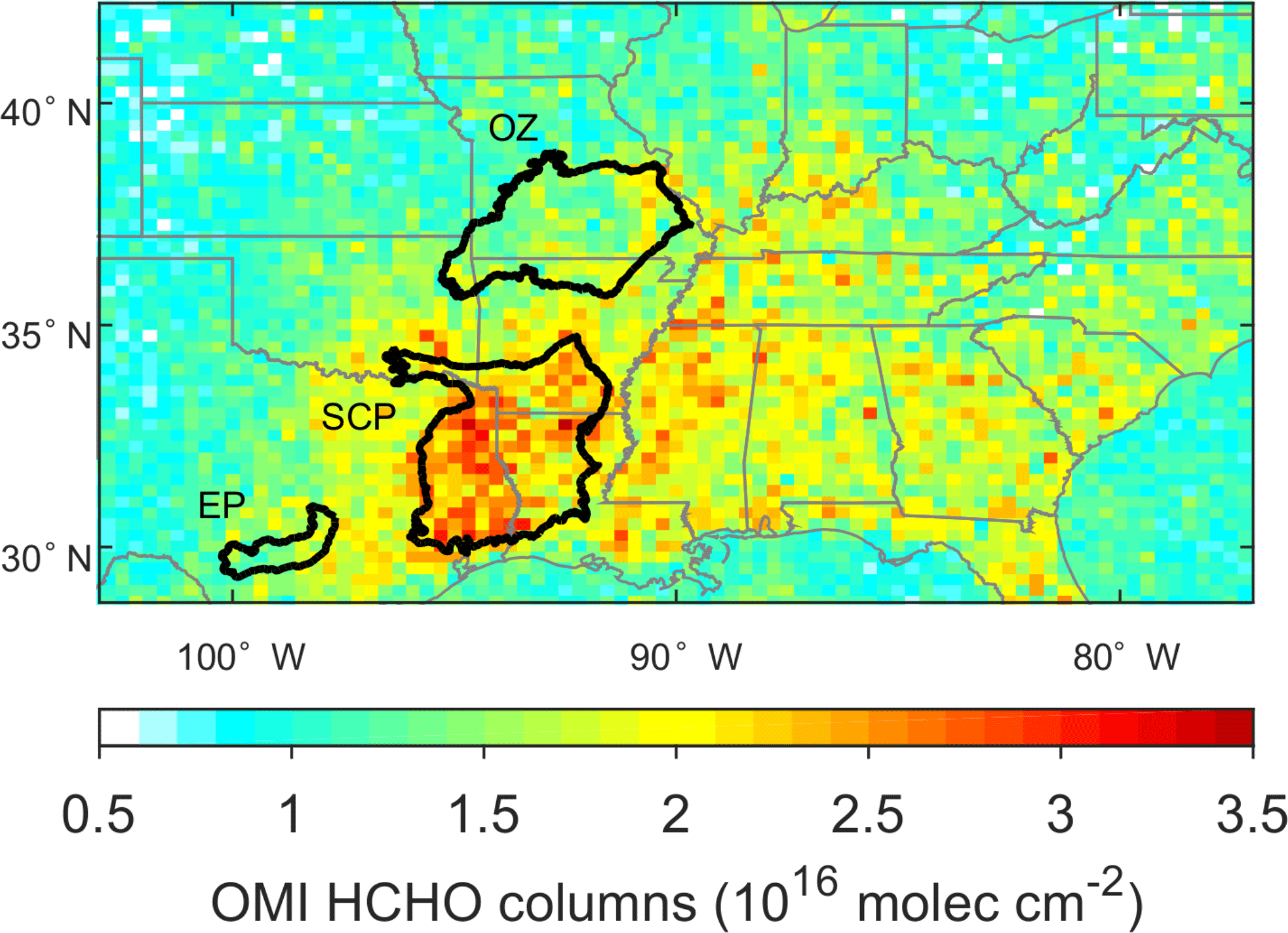
Figure 1Error-weighted mean OMI HCHO vertical column densities for the SEAC4RS time period (1 August 2013 – 25 September 2013). The Edwards Plateau (EP), Ozarks (OZ), and South Central Plains (SCP) ecoregions are denoted by black outlines (https://www.epa.gov/eco-research/ecoregions, level 3 and 4 data).
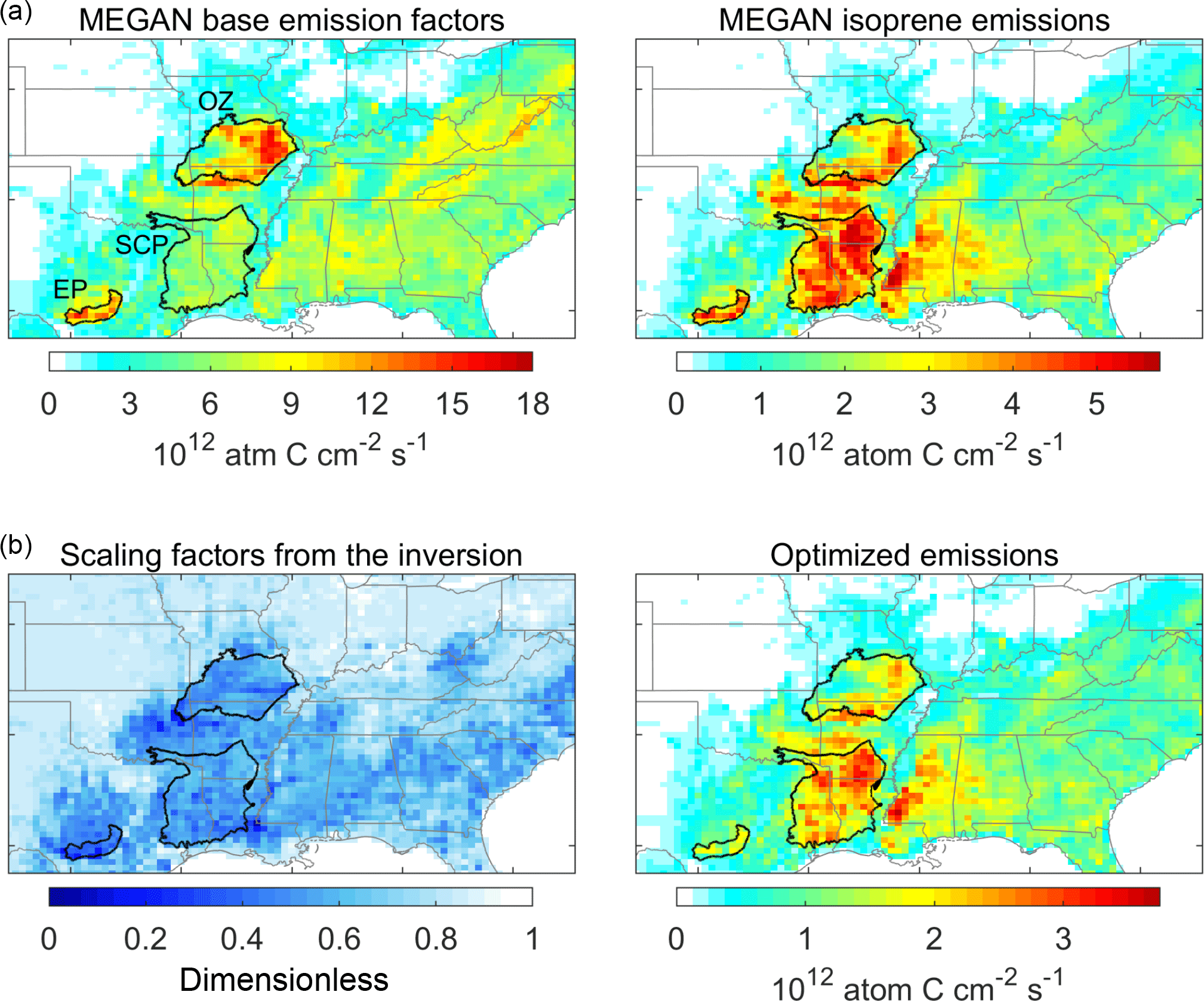
Figure 2Isoprene emissions in the southeast US. (a) MEGAN v2.1 base isoprene emission factors and emissions for the SEAC4RS time period. (b) Scaling factors from the inversion and optimized emissions. The color scale differs for MEGAN and optimized emissions. The Edwards Plateau (EP), Ozarks (OZ), and South Central Plains (SCP) ecoregions are denoted by black outlines.
Actual isoprene emissions are computed locally by multiplying the base emission factors by environmental factors to account for local conditions of leaf area index and leaf age, derived from MODIS observations (Myneni et al., 2007), and temperature and direct and diffuse solar radiation, taken from the GEOS-FP assimilated meteorological data used to drive GEOS-Chem. GEOS-FP temperatures in the boundary layer averaged 1 K higher than the SEAC4RS observations, and a downward correction is applied to the skin temperatures used in the computation of isoprene emissions in GEOS-Chem. The resulting emissions are shown in the top right panel of Fig. 2. The pattern differs from the base emission factors, primarily because of temperature. The highest emissions are in Louisiana and Arkansas, where temperatures are particularly high. The general spatial patterns of OMI HCHO (Fig. 1) and MEGAN v2.1 emissions show broad similarities but also substantial differences. For example, OMI shows no enhancement over the Edwards Plateau in Texas where MEGAN v2.1 predicts high isoprene emissions. These differences will be analyzed quantitatively in our inversion.
2.3 GEOS-Chem and its adjoint
We use the GEOS-Chem chemical transport model and its adjoint (Henze et al., 2007), driven by assimilated NASA GEOS-FP meteorological data in a nested configuration at 0.25∘ × 0.3125∘ horizontal resolution (Zhang et al., 2015, 2016; Kim et al., 2015). Our model domain covers the southeast US (102.812–77.188∘ W, 28.75–42.25∘ N; Fig. 1), taking initial and dynamic boundary conditions from a global simulation with 4∘ × 5∘ horizontal resolution. We simulate an 8-week period (1 August–25 September 2013) at the 0.25∘ × 0.3125∘ horizontal resolution.
The GEOS-Chem adjoint version is v35k, which is based on version v8 of GEOS-Chem with updates through v9 (http://acmg.seas.harvard.edu/geos). Here we update the chemical mechanism in v35k to GEOS-Chem v9.02 (Mao et al., 2010, 2013) and further update isoprene chemistry to GEOS-Chem v11-02 as described by Fisher et al. (2016) and Travis et al. (2016) in their simulation of SEAC4RS observations. These updates specifically include (1) explicit representation of isoprene peroxy radical (ISOPO2) isomerization and subsequent hydroperoxy-aldehyde (HPALD) formation, (2) formation of isoprene epoxides (IEPOX) and their oxidation, and (3) a 24 % increase in the HCHO yield from reaction of ISOPO2 with NO. The updated oxidation mechanism better reproduces the time- and NOx-dependence of HCHO production in the fully explicit Master Chemical Mechanism v3.3.1 (Jenkin et al., 2015) and agrees with the HCHO yields derived from SEAC4RS and SENEX aircraft measurements over the southeastern US (Wolfe et al., 2016; Chan Miller et al., 2017; Marvin et al., 2017).
US anthropogenic emissions in GEOS-Chem are from the 2011 National Emissions Inventory (NEI11) of the US Environmental Protection Agency, scaled to 2013 (EPA NEI, 2015). We decrease all anthropogenic sources of NOx other than power plants by 60 %, resulting in a total reduction of 50 %. Travis et al. (2016) showed this to be necessary in order to reproduce SEAC4RS and other 2013 observations for NOx and its oxidation products including OMI observations of NO2. Subsequent work has supported this downward correction of US anthropogenic NOx emissions (Chan Miller et al., 2017; Lin et al., 2017; McDonald et al., 2018). Soil NOx emissions are reduced by 50 % across the midwestern US as in Travis et al. (2016), based on previous analysis of OMI NO2 observations (Vinken et al., 2014). We note that Wolfe et al. (2015) found GEOS-Chem soil NO emissions to be too low over the Ozarks. Fire emissions, lightning NOx emissions, soil NOx emissions, non-isoprene MEGAN emissions, and updates to deposition are as in Travis et al. (2016). GEOS-FP diagnosed mixing depths are reduced by 40 % to better match aerosol lidar observations during SEAC4RS (Zhu et al., 2016).
2.4 Inversion approach
The state vector x to be optimized in the inversion consists of temporally invariant scaling factors on the 0.25∘ × 0.3125∘ GEOS-Chem grid applied to the prior MEGAN v2.1 isoprene emissions for the August – September 2013 SEAC4RS period. It consists of 4138 elements covering the land grid cells of the domain in Fig. 1. Zhu et al. (2016) previously found that decreasing MEGAN v2.1 emissions by 15 % improved the simulation of SEAC4RS HCHO observations and we include this correction in our prior estimate. Non-methane VOCs other than isoprene contribute less than 20 % to the HCHO column enhancements over the southeast US (Palmer et al., 2003; Millet et al., 2006) and are not optimized as part of the inversion.
The observation vector y consists of daily OMI HCHO columns (VCDs) calculated from OMI SCDs and GEOS-Chem AMFs mapped onto the 0.25∘ × 0.3125∘ GEOS-Chem grid. We relate y to x using GEOS-Chem, denoted as F and representing the forward model for the inversion:
GEOS-Chem HCHO columns are sampled at the OMI overpass time and filtered according to the same requirements outlined in Sect. 2.1. The observational error vector εO includes contributions from the forward model error, the representation error, and the measurement error (Brasseur and Jacob, 2017). The representation error can be neglected here because the GEOS-Chem resolution is commensurate with the size of OMI pixels, and the forward model error is expected to be small compared to the ∼ 80 % measurement error for individual scenes. Thus we take the measurement error as given in Sect. 2.1 to represent the observational error. The resulting observational error standard deviation averages 1.5 × 10¹⁶ molecules cm−2 for the domain of the inversion.
Assuming Gaussian error distributions and applying Bayes' theorem to weigh the information from the observations and the prior estimate, the solution to the optimization problem involves minimization of the cost function J(x) (Brasseur and Jacob, 2017):
where is the prior estimate for x, SA is the corresponding prior error covariance matrix, and is the observational error covariance matrix. We construct the prior error covariance matrix SA by assuming 100 % uncertainty in bottom-up emissions with no spatial error correlation. The sensitivity of the inversion to our assumptions for SA and SO will be tested in what follows.
The adjoint-based inversion enables a computationally tractable solution to the minimization of the cost function (3) when the forward model is highly non-linear, as is the case here. Starting from xA as a first guess, the GEOS-Chem adjoint model calculates the local gradient of the cost function (∇J(xA)) and passes it through the L-BFGS-B algorithm (Byrd et al., 1995; Zhu et al., 1997) to determine a next guess x1. It then recomputes (∇J(x1)) and so on until convergence to the optimal value. Convergence is reached when the cost function decreases by less than 1 % over three consecutive iterations.
2.5 Error analysis
We examined the sensitivity of the inversion results to different assumptions made regarding the specification of errors. In the first and all subsequent sensitivity analyses, we use the reported spectral fitting error in the operational retrieval without the factor of 1.59 increase. This gives an average observational error standard deviation of 0.9 × 10¹⁶ molecules cm−2, 40 % smaller than in the base case.
Our assumed prior error estimate of 100 % on the MEGAN v2.1 isoprene emissions in the base inversion is deliberately large to allow for the possibility of emissions being misplaced on the 0.25∘ × 0.3125∘ grid. We conducted a sensitivity analysis with a 50 % prior error estimate.
The prior errors in the base inversion have no spatial error correlation (i.e., SA is diagonal), but some error correlation may in fact be expected depending on the homogeneity of land cover types. To test this, we conducted a sensitivity simulation where the state vector x of emission scaling factors is not optimized on the 0.25∘ × 0.3125∘ grid but instead on a coarser irregular grid defined using a hierarchical clustering algorithm (Johnson, 1967; Wecht et al., 2014) with geographical proximity and commonality of MEGAN v2.1 emissions as clustering parameters. The resulting state vector is composed of 500 clusters, ∼ 10 times fewer than the number of grid cells at 0.25∘ × 0.3125∘ resolution.
A general assumption in Bayesian optimization is that observational errors are randomly distributed, as opposed to systematic bias. Previous analyses of SEAC4RS observations provide some confidence as to this lack of bias. The validation work of Zhu et al. (2016) led to removal of bias from the OMI HCHO satellite data. The work of Travis et al. (2016) and Fisher et al. (2016) removed bias in the GEOS-Chem simulation relating isoprene emission to HCHO production. GEOS-FP biases in temperature and mixing depths were corrected by Fisher et al. (2016) and Zhu et al. (2016), respectively. All of these corrections have been implemented in our simulation.
3.1 Optimal estimate of isoprene emissions
Figure 2 shows optimized scaling factors for our base inversion, and the resulting isoprene emissions (optimized emissions = MEGAN emissions × scaling factors). Isoprene emissions are lower than MEGAN v2.1 by 40 % on a regional average over the southeast US domain, with decreases of more than a factor of 3 in some areas. Figure 3 summarizes the results from the sensitivity analyses with different error assumptions. The base inversion and the different sensitivity analyses show similar spatial patterns for emissions, with correlation coefficients r=0.96–0.98 on the 0.25∘ × 0.3125∘ grid. The decrease in total regional emissions relative to MEGAN v2.1 ranges between 40 and 54 %. The cluster inversion shows the largest decrease, because the smaller-dimension state vector allows for a stronger fit from observations. However, aggregation errors in that inversion could cause overfit (Turner and Jacob, 2015).
Figure 4 shows the simulated HCHO columns from GEOS-Chem using the MEGAN v2.1 emissions and using the optimized emissions from the base inversion (Fig. 2). The positive bias over high isoprene emitting regions using MEGAN v2.1 disappears when using the optimized emissions. The negative bias (−3 × 10¹⁵ molecules cm−2) that persists over low-isoprene emitting regions is not corrected due to the high error associated with the OMI observations and the low isoprene emissions in those regions. We attribute this to a bias in the background, unrelated to isoprene emission. The best agreement between OMI and GEOS-Chem is provided by the base inversion configuration, as shown in Figs. 2 and 4. The base inversion also provides the best agreement with SEAC4RS data, as presented below.
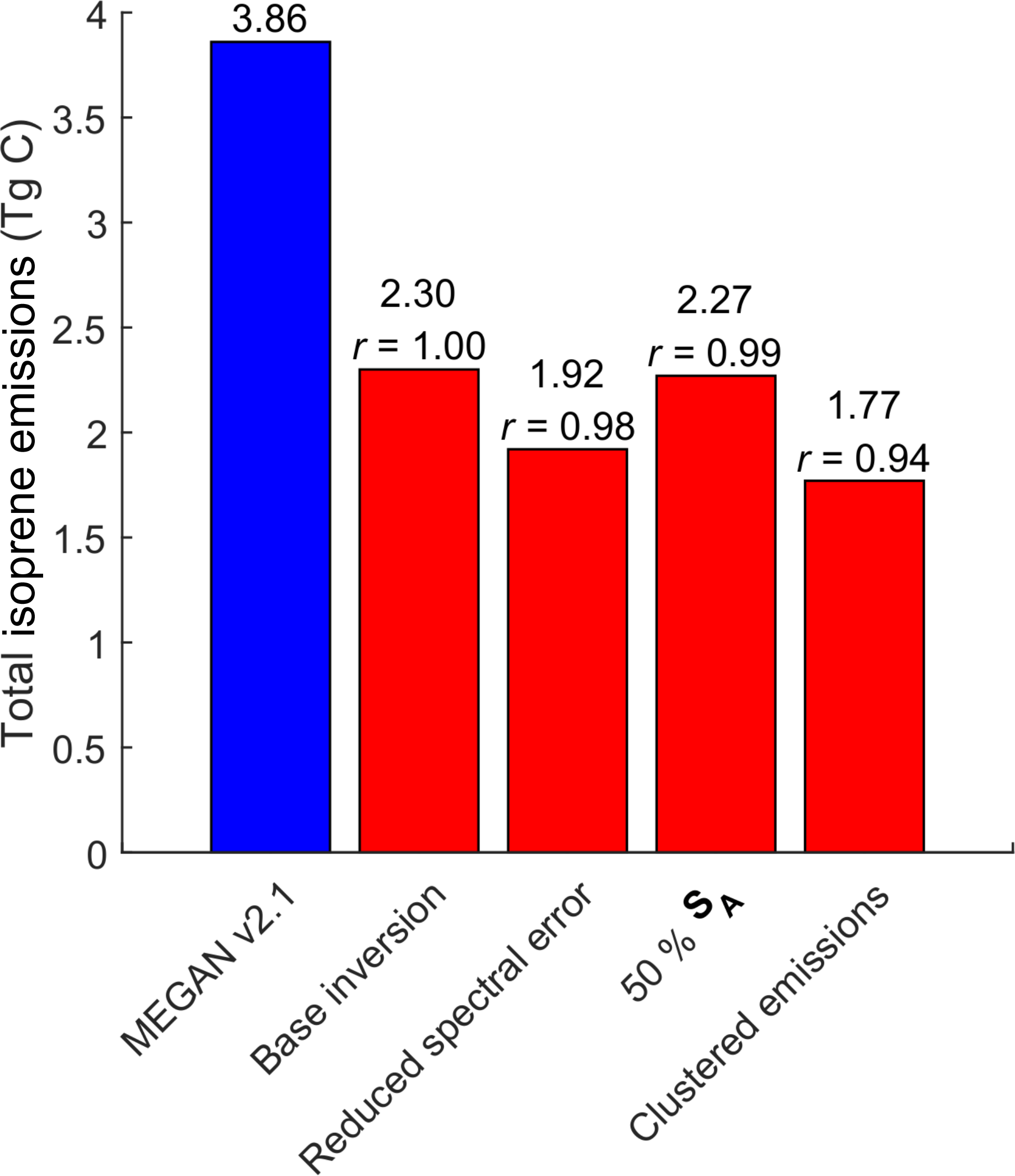
Figure 3Total isoprene emissions for the southeast US domain of Fig. 1 over the period 1 August – 25 September 2013. The MEGAN v2.1 inventory value is compared to results from the base inversion applied to the OMI formaldehyde data (optimized emissions in Fig. 2) and to sensitivity inversions using different error specifications (see text for details). Numbers on top of each bar are the total isoprene emissions, and correlation coefficients (r) describe the spatial consistency between the base inversion (r=1) and the sensitivity inversions.
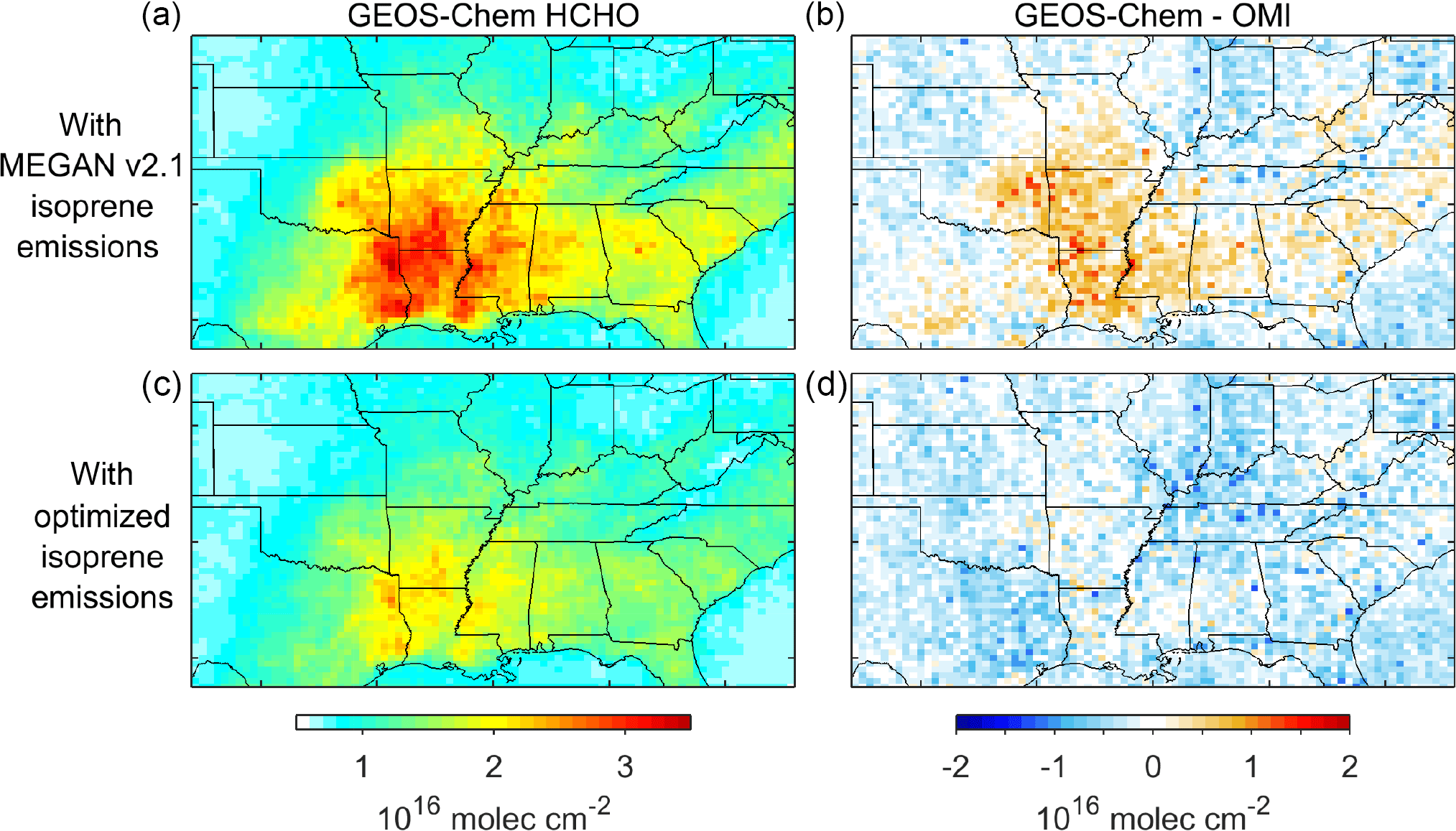
Figure 4Simulated HCHO vertical column densities and model bias using prior and optimized isoprene emissions. Values are averages for 1 August – 25 September 2013 at the OMI overpass time (13:30 LT), weighted by the OMI measurement error as in Fig. 1. (b) and (d) show the differences between the simulated columns and the OMI observations from Fig. 1.
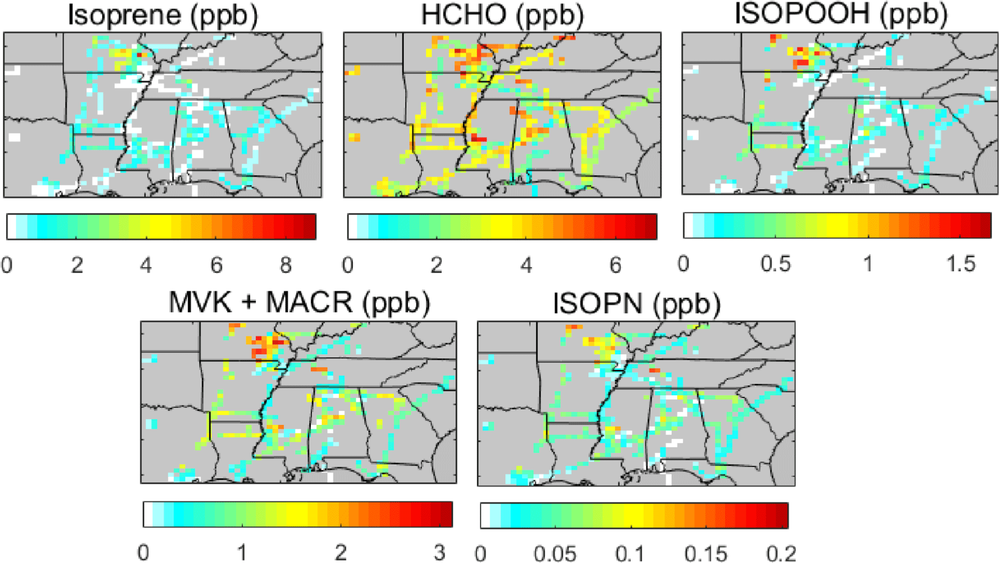
Figure 5Mean boundary layer concentrations of isoprene and its oxidation products measured in the SEAC4RS aircraft campaign (1 August – 25 September 2013). The observations are for daytime (09:00 – 18:00 LT) below 1.5 km altitude, and exclude urban and fire plumes as described in the text.
3.2 Comparisons with SEAC4RS data
In situ measurements of isoprene and its oxidation products aboard the SEAC4RS aircraft provide an independent test of the inversion results. HCHO was measured in SEAC4RS via two different techniques: mid-IR absorption spectroscopy using the CAMS (Richter et al., 2015), and laser-induced fluorescence using the NASA GSFC ISAF (Cazorla et al., 2015). The two measurements are well correlated (r=0.96 in the mixed layer), with ISAF ∼ 10 % higher than CAMS measurements (Zhu et al., 2016). Here we use the CAMS measurements, as these measurements were used in the validation of the OMI SAO product (Zhu et al., 2016). The associated measurement uncertainty is 4 %. Isoprene and the sum of methyl vinyl ketone and methacrolein (MVK+MACR) were measured by PTR-MS (de Gouw and Warneke, 2007), with reported uncertainties of 5 and 10 %, respectively. Isoprene hydroperoxides (ISOPOOH) and isoprene nitrates (ISOPN) were measured by the Caltech CIMS (Crounse et al., 2006; Paulot et al., 2009; St. Clair et al., 2010), with respective uncertainties of 30 ppt + 40 % and 10 ppt + 30 %.
MVK+MACR measurements are corrected to account for the interference caused by the degradation of ISOPOOH on instrument surfaces (Rivera-Rios et al., 2014). The correction is calculated as MVK+MACRcorrected = MVK+MACRmeasured − X × ISOPOOHmeasured, where X = 0.44 with a relatively large uncertainty of . Formaldehyde measurements may suffer from a similar, but smaller interference. In the ISAF instrument, conversion of ISOPOOH to HCHO contributes negligibly (< 4 %) to the observed signal in ISOPOOH- and HCHO-rich environments, but a delay in ISOPOOH conversion and a rapid transition in sampling environments can manifest in more substantial (< 10 %) interferences (St. Clair et al., 2016). This has not yet been examined for the CAMS instrument.
We exclude data influenced by urban plumes ([NO2] > 4 ppb), open fire plumes ([CH3CN] > 200 ppt), and stratospheric air ([O3] ∕ [CO] > 1.25 mol mol−1), and focus solely on measurements within the daytime boundary layer (09:00–18:00 LT, < 1.5 km). In all comparisons with model results, observations are averaged over the GEOS-Chem grid at 10 min time steps.
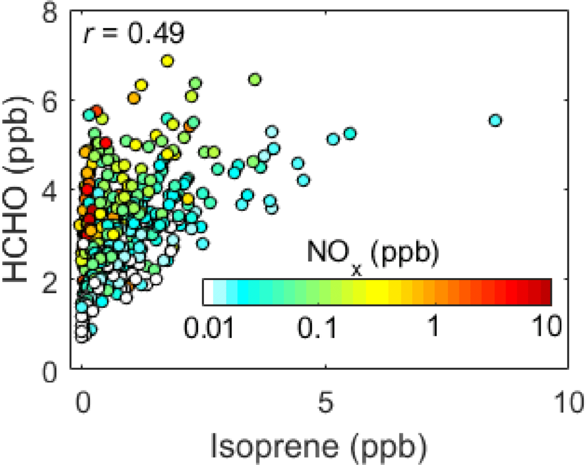
Figure 6Relationship of boundary layer isoprene and HCHO measured during SEAC4RS, colored by observed NOx. Data are the same as in Fig. 5.

Figure 7Comparison of SEAC4RS observations and modeled mixing ratios using either MEGAN v2.1 (blue) or the optimized isoprene emissions (red) from the base inversion of OMI HCHO data (Fig. 2). The dashed line indicates 1:1 agreement. The colored lines are the reduced major axis linear regressions and the inset numbers are the corresponding slopes, with error standard deviations inferred from bootstrap sampling.
Figure 5 shows the distribution of SEAC4RS observations. The aircraft flew over the Ozarks on several hot days, leading to the particularly high concentrations of isoprene and its oxidation products in the region. ISOPOOH is produced by the low-NOx pathway for isoprene oxidation, while ISOPN is produced by the high-NOx pathway. MVK and MACR are produced mostly by the high-NOx pathway. The spatial patterns reflect the contributions of both pathways across the southeast US (Travis et al., 2016). Formaldehyde is more distributed because of the time lag in HCHO production from isoprene emission (Chan Miller et al., 2017). The relatively low correlation between isoprene and formaldehyde (r=0.49, Fig. 6) illustrates the importance of accounting for transport in inversions of HCHO data to infer isoprene emissions at fine resolution.
Figure 7 compares observed mixing ratios for isoprene and its oxidation products to the values simulated by GEOS-Chem using either MEGAN v2.1 isoprene emissions or the optimal estimate from the inversion. MEGAN v2.1 emissions lead to a factor of 2.5 overestimate in SEAC4RS observations of isoprene and ISOPOOH, a 50 % overestimate in HCHO, factor of 2 overestimate for MVK+MACR, and 20 % overestimate for ISOPN. The optimal estimate decreases the simulated concentrations and produces agreement with all observations within measurement uncertainty. The effect on isoprene and ISOPOOH is particularly large because the correction of emissions is strongest in high-emitting regions, which happen to also have low NOx (Fig. 6; Yu et al., 2016). The reduction in HCHO, MVK+MACR, and ISOPN is less pronounced. Zhu et al. (2016) previously found no GEOS-Chem model bias relative to the SEAC4RS HCHO observations using MEGAN v2.1 emissions reduced by a uniform 15 %, but they used an older GEOS-Chem version that did not include updates to anthropogenic emissions, deposition, the isoprene oxidation mechanism (including a higher HCHO yield from the ISOPO2 + NO reaction), and the inclusion of alpha-pinene and limonene oxidation. Travis et al. (2016) previously reported a factor of 2 overestimate of ISOPOOH in their SEAC4RS simulation with MEGAN v2.1 reduced by 15 %, and the lower emissions in our optimal estimate effectively correct that bias.
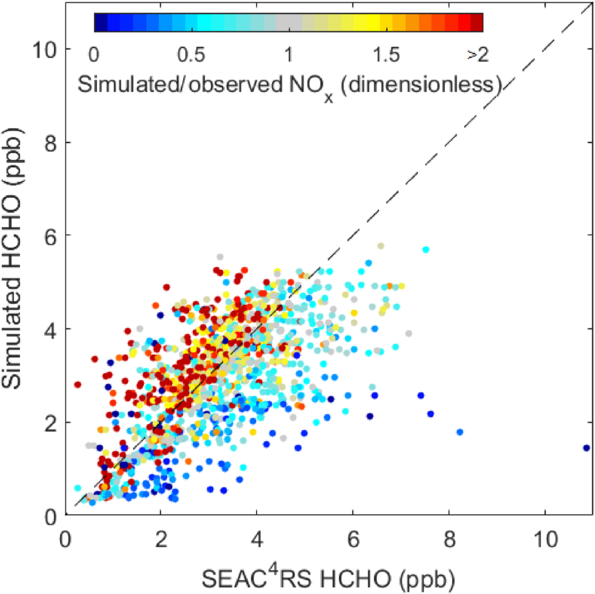
Figure 8Comparison of simulated and observed HCHO concentrations along the SEAC4RS flight tracks, using the model with optimized isoprene emissions from the base inversion. The dashed line indicates 1:1 agreement. Data are the same as in Fig. 7 (upper middle) but are colored by the local ratio of simulated to observed NOx concentration.
Much of the residual scatter in the comparison of simulated vs. observed HCHO using optimized isoprene emissions appears to be caused by local bias in NOx (Fig. 8). There is no mean NOx bias in our inversion (Travis et al., 2016) but there can be local bias. We find that local model biases in simulating HCHO observations are strongly correlated with corresponding model errors in NOx, reflecting the NOx-dependence of HCHO production from isoprene (Fig. 6 and Chan Miller et al., 2017). When excluding points with more than 50 % error in NOx, the correlation between measured and simulated HCHO improves from r=0.62 to r=0.70 (n=1222 to n=708). This emphasizes the importance for inversions of HCHO data to use unbiased NOx concentrations.
Our results indicate that MEGAN v2.1 isoprene emissions over the southeast US should be decreased by an average of 40 %, consistent with previous analyses of OMI HCHO data which inferred 25–50 % decreases (Millet et al., 2008; Bauwens et al., 2016). MEGAN v2.1 isoprene emissions are typically a factor of 2 higher than the emissions calculated from the BEIS3 inventory often used in US air quality models (Warneke et al., 2010; Carlton and Baker, 2011). BEIS and MEGAN both follow the emissions algorithms outlined in Guenther et al. (2006), but they use different canopy models and base emission factors (Bash et al., 2016). The geographic specificity of our high-resolution inversion allows us to examine potential causes of the MEGAN v2.1 overestimate in various environments. Below, we discuss three ecoregions in greater detail.
The high base isoprene emission factors in the Ozarks ecoregion (Fig. 2) have to led this region being dubbed the “isoprene volcano” (Wiedinmyer et al., 2005). We find a 46 % reduction in emissions in the region relative to MEGAN v2.1, in good agreement with isoprene flux measurements from SEAC4RS (Wolfe et al., 2015). Independent aircraft measurements over the southeast US during the summer of 2013 found that MEGAN v2.1 was biased high by a factor of two for mixed pine–oak forests typical of the Ozarks (Yu et al., 2017). These authors suggest that non-emitting trees in the upper canopy may shade emitting trees, leading to lower than anticipated isoprene emissions.
The hot spot of isoprene emissions in the South Central Plains (Fig. 2) is also reduced by 48 % in our inversion relative to MEGAN v2.1. This region is dominated by needle leaf trees, with isoprene emissions stemming from the sweetgum–tupelo understory. Again, vertical heterogeneity or an incorrect fraction of emitters could lead to the MEGAN overestimate of emissions. Alternatively, the base emission factor of sweetgum and tupelo could be significantly less than the assigned MEGAN value.
The Edwards Plateau in central Texas is a major isoprene source region in MEGAN v2.1, with base emission factors as high as in the Ozarks (Fig. 2), but our inversion decreases emissions in that region by more than a factor of 3. A land cover map used for BEIS (BELD4) shows no isoprene emission hotspot in the region (Wang et al., 2017), consistent with our result. Both land cover maps are derived from the NLCD, but they follow different methodologies for translating NLCD classifications to base emission factors. NLCD-based maps show the Edwards Plateau dominated by broadleaf trees, whereas the MODIS land cover product is dominated by grasses, leading to a factor of 10 lower isoprene emissions (Huang et al., 2015). Uncertainty in the dependence of isoprene emission on soil moisture could also affect isoprene emission estimates for the Edwards Plateau (Sindelarova et al., 2014).
Isoprene emissions can either increase or decrease surface ozone in air quality models, depending on the local chemical environment and the chemical mechanism used (Mao et al., 2013). We find in GEOS-Chem that our optimized isoprene emissions lead to a decrease in mean surface afternoon O3 concentrations by ∼ 1–3 ppb over the southeast US relative to the simulation using MEGAN v2.1 emissions. The GEOS-Chem simulation of Travis et al. (2016) previously found an 8 ppb overestimate of surface ozone over the southeast US during SEAC4RS; excessive isoprene emissions could contribute.
Isoprene is also a precursor for organic aerosol (OA), which is a dominant contributor to fine particulate matter (PM2.5) in surface air (Zhang et al., 2007). Kim et al. (2015) found in their GEOS-Chem simulation of the SEAC4RS period that isoprene contributes 40 % of total OA over the southeast US in summer, assuming a 3 % mass yield from isoprene oxidation and MEGAN v2.1 isoprene emissions reduced by 15 %. A more mechanistic study of OA formation from isoprene oxidation under the SEAC4RS conditions found a 3.3 % mass yield, most of which was produced in the low-NOx pathway (Marais et al., 2016). Our work finds a factor of 2 decrease in ISOPOOH relative to the simulation using MEGAN v2.1 emissions reduced by 15 %, and consistent with observations (Fig. 6). This suggests that isoprene OA formation may be only half of the value found by Kim et al. (2015), implying that other sources such as terpenes may make more important contributions to OA (Pye et al., 2010, 2015; Xu et al., 2015; Zhang et al., 2018).
We used newly validated HCHO observations from the OMI satellite instrument to demonstrate the capability for applying these satellite observations to fine-resolution inversion of isoprene emissions from vegetation. Our work focused on the southeast US where aircraft observations from the NASA SEAC4RS campaign provide detailed chemical information on isoprene and its oxidation products (including HCHO) to independently evaluate the inversion. The inversion used the adjoint of the GEOS-Chem chemical transport model at 0.25∘ × 0.3125∘ horizontal resolution and leveraged on previous studies that applied GEOS-Chem to simulation of the SEAC4RS observations including in particular for NOx. HCHO yields from isoprene oxidation are highly sensitive to NOx levels, and the high resolution of the GEOS-Chem inversion allowed us to properly describe the spatial segregation between isoprene and NOx emissions.
We found that the MEGAN v2.1 inventory of isoprene emissions commonly used in atmospheric chemistry models is biased high on average by 40 % across the southeast US. This is consistent with several previous top-down studies and recent analyses using flight-based flux and eddy covariance measurements. Our optimized emissions produce better agreement with SEAC4RS observations of isoprene and its oxidation products including HCHO. Local model errors in simulating HCHO observations along the aircraft flight tracks are highly correlated with local model errors in NOx. This highlights the importance of accurate NOx fields in inversions of HCHO observations to infer isoprene emissions.
The high resolution of our inversion allows us to quantify isoprene emissions and analyze MEGAN v2.1 biases on ecosystem-relevant scales. We find that MEGAN v2.1 is biased high everywhere across the southeast US but is correct in placing maximum 2013 emissions in Arkansas, Louisiana, and Mississippi. The Ozarks Plateau in southeast Missouri has particularly high base emission factors in MEGAN v2.1, reflecting the abundance of oak trees, but isoprene emissions there are dampened by relatively low temperatures and our results further suggest an overestimate in the base emission factors. Another prominent overestimate is over the Edwards Plateau in central Texas where MEGAN v2.1 emissions are biased high by a factor of 3, possibly reflecting errors in land cover. Our results suggest that the BEIS inventory may yield more accurate isoprene emissions for these areas.
Our downward correction of isoprene emissions in GEOS-Chem as a result of the inversion leads to a 1–3 ppb reduction in modeled surface O3, correcting some of the overestimate previously found in the model. It also decreases the contribution of isoprene to organic aerosol, possibly suggesting a greater role for terpenes.
HCHO observations from space are expected to improve considerably in the near future. TROPOMI, launched in October 2017 will provide global HCHO and NO2 observations at 7 km × 7 km nadir resolution daily (Veefkind et al., 2012), as compared to 24 km × 13 km for OMI. Concurrent HCHO and NO2 observations can provide a check against model bias in NOx affecting the yield of HCHO from isoprene (Marais et al., 2012). The TEMPO geostationary instrument to be launched in the 2019 – 2022 window will provide HCHO and NO2 observations at 2 km × 4.5 km pixel resolution multiple times per day (Zoogman et al., 2017). Coupled with the high-resolution inversion framework shown here, these future observations may greatly improve our ability to quantify US isoprene emissions from space.
The OMI-SAO Version-3 Formaldehyde Product is available at the NASA Goddard Earth Sciences Data and Information Services Center (Chance, 2007). SEAC4RS observations are available from the NASA LaRC Airborne Science Data for Atmospheric Composition (SEAC4RS Science Team, 2014).
The authors declare that they have no conflict of interest.
We are grateful for the contributions from all members of the SEAC4RS
flight and science teams. We acknowledge Thomas B. Ryerson for his
contribution of the NOx measurements. Tomas Mikoviny is acknowledged for
his support with the PTR-MS data acquisition and analysis. PTR-MS
measurements during SEAC4RS were supported by the Austrian Federal Ministry
for Transport, Innovation and Technology (bmvit) through the Austrian Space
Applications Programme (ASAP) of the Austrian Research Promotion
Agency (FFG). Funding was provided by the NASA Aura Science Team.
Edited by: Qiang Zhang
Reviewed by: two anonymous referees
Abbot, D., Palmer, P., Martin, R., Chance, K., Jacob, D., and Guenther, A.: Seasonal and interannual variability of isoprene emissions as determined by formaldehyde column measurements from space, Geophys. Res. Lett., 17, 1886, https://doi.org/10.1029/2003GL017336, 2003.
Arneth, A., Monson, R. K., Schurgers, G., Niinemets, U., and Palmer, P. I.: Why are estimates of global terrestrial isoprene emissions so similar (and why is this not so for monoterpenes)?, Atmos. Chem. Phys., 8, 4605–4620, https://doi.org/10.5194/acp-8-4605-2008, 2008.
Barkley, M. P., Smedt, I. D., Van?Roozendael, M., Kurosu, T. P., Chance, K., Arneth, A., Hagberg, D., Guenther, A., Paulot, F., Marais, E., and Mao, J.: Top-down isoprene emissions over tropical South America inferred from SCIAMACHY and OMI formaldehyde columns, J. Geophys. Res.-Atmos., 118, 6849–6868, https://doi.org/10.1002/jgrd.50552, 2013.
Bash, J. O., Baker, K. R., and Beaver, M. R.: Evaluation of improved land use and canopy representation in BEIS v3.61 with biogenic VOC measurements in California, Geosci. Model Dev., 9, 2191–2207, https://doi.org/10.5194/gmd-9-2191-2016, 2016.
Bauwens, M., Stavrakou, T., Müller, J.-F., De Smedt, I., Van Roozendael, M., van der Werf, G. R., Wiedinmyer, C., Kaiser, J. W., Sindelarova, K., and Guenther, A.: Nine years of global hydrocarbon emissions based on source inversion of OMI formaldehyde observations, Atmos. Chem. Phys., 16, 10133–10158, https://doi.org/10.5194/acp-16-10133-2016, 2016.
Boeke, N. L., Marshall, J. D., Alvarez, S., Chance, K. V., Fried, A., Kurosu, T. P., Rappenglueck, B., Richter, D., Walega, J., Weibring, P., and Millet, D. B.: Formaldehyde columns from the Ozone Monitoring Instrument: Urban versus background levels and evaluation using aircraft data and a global model, J. Geophys. Res., 116, D05303, https://doi.org/10.1029/2010JD014870, 2011.
Brasseur, G. P. and Jacob, D. J.: Modeling of Atmospheric Chemistry, Cambridge University Press, Cambridge, UK, 487–533, 2017.
Byrd, R. H., Lu, P., Nocedal, J., and Zhu, C.: A limited memory algorithm for bound constrained optimization, Sci. Comput., 16, 1190–1208, https://doi.org/10.1137/0916069, 1995.
Carlton, A. G. and Baker, K.: Photochemical modeling of the Ozark isoprene volcano: MEGAN, BEIS and their impacts on air quality predictions, Environ. Sci. Tech., 45, 4438–4445, 2011.
Carlton, A. G., Wiedinmyer, C., and Kroll, J. H.: A review of Secondary Organic Aerosol (SOA) formation from isoprene, Atmos. Chem. Phys., 9, 4987–5005, https://doi.org/10.5194/acp-9-4987-2009, 2009.
Cazorla, M., Wolfe, G. M., Bailey, S. A., Swanson, A. K., Arkinson, H. L., and Hanisco, T. F.: A new airborne laser-induced fluorescence instrument for in situ detection of formaldehyde throughout the troposphere and lower stratosphere, Atmos. Meas. Tech., 8, 541–552, https://doi.org/10.5194/amt-8-541-2015, 2015.
Chan Miller, C., Jacob, D. J., Marais, E. A., Yu, K., Travis, K. R., Kim, P. S., Fisher, J. A., Zhu, L., Wolfe, G. M., Hanisco, T. F., Keutsch, F. N., Kaiser, J., Min, K. E., Brown, S. S., Washenfelder, R. A., González Abad, G., and Chance, K.: Glyoxal yield from isoprene oxidation and relation to formaldehyde: chemical mechanism, constraints from SENEX aircraft observations, and interpretation of OMI satellite data, Atmos. Chem. Phys., 17, 8725–8738, https://doi.org/10.5194/acp-17-8725-2017, 2017.
Chance, K.: OMI/Aura Formaldehyde (HCHO) Total Column 1-orbit L2 Swath 13x24 km V003, Goddard Earth Sciences Data and Information Services Center (GES DISC), https://doi.org/10.5067/Aura/OMI/DATA2015 (last access: February 2017), 2007.
Crounse, J. D., McKinney, K. A., Kwan, A. J., and Wennberg, P. O.: Measurement of gas-phase hydroperoxides by chemical ionization mass spectrometry (CIMS), Anal. Chem., 78, 6726–6732, 2006.
de Gouw, J. and Warneke, C.: Measurements of volatile organic compounds in the earths atmosphere using proton-transferreaction mass spectrometry, Mass Spec. Rev., 26, 223–257, https://doi.org/10.1002/mas.20119, 2007.
EPA NEI (National Emissions Inventory v11): Air Pollutant Emission Trends Data: http://www.epa.gov/ttn/chief/trends/index.html (last access: 23 June 2015), 2015.
Fiore, A. M., Horowitz, L. W., Purves, D. W., Levy, H., Evans, M. J., Wang, Y. X., Li, Q. B., and Yantosca, R. M.: Evaluating the contribution of changes in isoprene emissions to surface ozone trends over the eastern United States, J. Geophys. Res.-Atmos., 110, D12303, https://doi.org/10.1029/2004jd005485, 2005.
Fisher, J. A., Jacob, D. J., Travis, K. R., Kim, P. S., Marais, E. A., Chan Miller, C., Yu, K., Zhu, L., Yantosca, R. M., Sulprizio, M. P., Mao, J., Wennberg, P. O., Crounse, J. D., Teng, A. P., Nguyen, T. B., St. Clair, J. M., Cohen, R. C., Romer, P., Nault, B. A., Wooldridge, P. J., Jimenez, J. L., Campuzano-Jost, P., Day, D. A., Hu, W., Shepson, P. B., Xiong, F., Blake, D. R., Goldstein, A. H., Misztal, P. K., Hanisco, T. F., Wolfe, G. M., Ryerson, T. B., Wisthaler, A., and Mikoviny, T.: Organic nitrate chemistry and its implications for nitrogen budgets in an isoprene- and monoterpene-rich atmosphere: constraints from aircraft (SEAC4RS) and ground-based (SOAS) observations in the Southeast US, Atmos. Chem. Phys., 16, 5969–5991, https://doi.org/10.5194/acp-16-5969-2016, 2016.
Fortems-Cheiney, A., Chevallier, F., Pison, I., Bousquet, P., Saunois, M., Szopa, S., Cressot, C., Kurosu, T. P., Chance, K., and Fried, A.: The formaldehyde budget as seen by a global-scale multi-constraint and multi-species inversion system, Atmos. Chem. Phys., 12, 6699–6721, https://doi.org/10.5194/acp-12-6699-2012, 2012.
González Abad, G., Liu, X., Chance, K., Wang, H., Kurosu, T. P., and Suleiman, R.: Updated Smithsonian Astrophysical Observatory Ozone Monitoring Instrument (SAO OMI) formaldehyde retrieval, Atmos. Meas. Tech., 8, 19–32, https://doi.org/10.5194/amt-8-19- 2015, 2015.
Guenther, A., Karl, T., Harley, P., Wiedinmyer, C., Palmer, P. I., and Geron, C.: Estimates of global terrestrial isoprene emissions using MEGAN (Model of Emissions of Gases and Aerosols from Nature), Atmos. Chem. Phys., 6, 3181–3210, https://doi.org/10.5194/acp-6-3181-2006, 2006.
Guenther, A. B., Jiang, X., Heald, C. L., Sakulyanontvittaya, T., Duhl, T., Emmons, L. K., and Wang, X.: The Model of Emissions of Gases and Aerosols from Nature version 2.1 (MEGAN2.1): an extended and updated framework for modeling biogenic emissions, Geosci. Model Dev., 5, 1471–1492, https://doi.org/10.5194/gmd-5-1471-2012, 2012.
Henze, D. K., Hakami, A., and Seinfeld, J. H.: Development of the adjoint of GEOS-Chem, Atmos. Chem. Phys., 7, 2413–2433, https://doi.org/10.5194/acp-7-2413-2007, 2007.
Hogrefe, C., Isukapalli, S., Tang, X., Georgopoulos, P., He, S., Zalewsky, E., Hao, W., Ku, J., Key, T., and Sistla, G.: Impact of biogenic emission uncertainties on the simulated response of ozone and fine Particulate Matter to anthropogenic emission reductions, J. Air Waste Manage., 61, 92–108, 2011.
Homer, C. G., Huang, C., Yang, L., Wylie, B. K., and Coan, M.: Development of a 2001 National Land Cover Database for the United States, Photogramm. Eng. Remote Sens., 70, 829–840, https://doi.org/10.14358/PERS.70.7.829, 2004.
Hu, L., Millet, D. B., Baasandorj, M., Griffis, T. J., Turner, P., Helmig, D., Curtis, A. J., and Hueber, J.: Isoprene emissions and impacts over an ecological transition region in the U.S. Upper Midwest inferred from tall tower measurements, J. Geophys. Res.-Atmos., 120, 3553–3571, https://doi.org/10.1002/2014JD022732, 2015.
Huang, L., McDonald-Buller, E., McGaughey, G., Kimura, Y., and Allen, D. T.: Comparison of regional and global land cover products and the implications for biogenic emission modeling, J. Air Waste Manage., 65, 1194–1205, https://doi.org/10.1080/10962247.2015.1057302, 2015.
Jenkin, M. E., Young, J. C., and Rickard, A. R.: The MCM v3.3.1 degradation scheme for isoprene, Atmos. Chem. Phys., 15, 11433–11459, https://doi.org/10.5194/acp-15-11433-2015, 2015.
Johnson, S. C.: Hierarchical clustering schemes, Psychometrika, 32, 241–254, 1967.
Kim, P. S., Jacob, D. J., Fisher, J. A., Travis, K., Yu, K., Zhu, L., Yantosca, R. M., Sulprizio, M. P., Jimenez, J. L., Campuzano-Jost, P., Froyd, K. D., Liao, J., Hair, J. W., Fenn, M. A., Butler, C. F., Wagner, N. L., Gordon, T. D., Welti, A., Wennberg, P. O., Crounse, J. D., St. Clair, J. M., Teng, A. P., Millet, D. B., Schwarz, J. P., Markovic, M. Z., and Perring, A. E.: Sources, seasonality, and trends of southeast US aerosol: an integrated analysis of surface, aircraft, and satellite observations with the GEOS-Chem chemical transport model, Atmos. Chem. Phys., 15, 10411–10433, https://doi.org/10.5194/acp-15-10411-2015, 2015.
Lin, M., Horowitz, L. W., Payton, R., Fiore, A. M., and Tonnesen, G.: US surface ozone trends and extremes from 1980 to 2014: quantifying the roles of rising Asian emissions, domestic controls, wildfires, and climate, Atmos. Chem. Phys., 17, 2943–2970, https://doi.org/10.5194/acp-17-2943-2017, 2017.
Mao, J., Jacob, D. J., Evans, M. J., Olson, J. R., Ren, X., Brune, W. H., St Clair, J. M., Crounse, J. D., Spencer, K. M., Beaver, M. R., Wennberg, P. O., Cubison, M. J., Jimenez, J. L., Fried, A., Weibring, P., Walega, J. G., Hall, S. R., Weinheimer, A. J., Cohen, R. C., Chen, G., Crawford, J. H., McNaughton, C., Clarke, A. D., Jaegle, L., Fisher, J. A., Yantosca, R. M., Le Sager, P., and Carouge, C.: Chemistry of hydrogen oxide radicals (HOx) in the Arctic troposphere in spring, Atmos. Chem. Phys., 10, 5823-5838, https://doi.org/10.5194/acp-10-5823-2010, 2010.
Mao, J. Q., Paulot, F., Jacob, D. J., Cohen, R. C., Crounse, J. D., Wennberg, P. O., Keller, C. A., Hudman, R. C., Barkley, M. P., and Horowitz, L. W.: Ozone and organic nitrates over the eastern United States: Sensitivity to isoprene chemistry, J. Geophys. Res.-Atmos., 118, 11256–11268, https://doi.org/10.1002/jgrd.50817, 2013.
Marais, E. A., Jacob, D. J., Kurosu, T. P., Chance, K., Murphy, J. G., Reeves, C., Mills, G., Casadio, S., Millet, D. B., Barkley, M. P., Paulot, F., and Mao, J.: Isoprene emissions in Africa inferred from OMI observations of formaldehyde columns, Atmos. Chem. Phys., 12, 6219–6235, https://doi.org/10.5194/acp-12-6219-2012, 2012.
Marais, E. A., Jacob, D. J., Guenther, A., Chance, K., Kurosu, T. P., Murphy, J. G., Reeves, C. E., and Pye, H. O. T.: Improved model of isoprene emissions in Africa using Ozone Monitoring Instrument (OMI) satellite observations of formaldehyde: implications for oxidants and particulate matter, Atmos. Chem. Phys., 14, 7693–7703, https://doi.org/10.5194/acp-14-7693-2014, 2014.
Marais, E. A., Jacob, D. J., Jimenez, J. L., Campuzano-Jost, P., Day, D. A., Hu, W., Krechmer, J., Zhu, L., Kim, P. S., Miller, C. C., Fisher, J. A., Travis, K., Yu, K., Hanisco, T. F., Wolfe, G. M., Arkinson, H. L., Pye, H. O. T., Froyd, K. D., Liao, J., and McNeill, V. F.: Aqueous-phase mechanism for secondary organic aerosol formation from isoprene: application to the southeast United States and co-benefit of SO2 emission controls, Atmos. Chem. Phys., 16, 1603–1618, https://doi.org/10.5194/acp-16-1603-2016, 2016.
Marvin, M. R., Wolfe, G. M., Salawitch, R. J., Canty, T. P., Roberts, S. J., Travis, K. R., Aikin, K. C., de Gouw, J. A., Graus, M., Hanisco, T. F., Holloway, J. S., Hübler, G., Kaiser, J., Keutsch, F. N., Peischl, J., Pollack, I. B., Roberts, J. M., Ryerson, T. B., Veres, P. R., and Warneke, C.: Impact of evolving isoprene mechanisms on simulated formaldehyde: An inter-comparison supported by in situ observations from SENEX, Atmos. Environ., 164, 325–336, https://doi.org/10.1016/j.atmosenv.2017.05.049, 2017.
McDonald, B. C., McKeen, S. A., Cui, Y., Ahmadov, R., Kim, S. W., Frost, G. J., Pollack, I. B., Ryerson, T. B., Holloway, J. S., Graus, M., Warneke, C., de Gouw, J. A., Kaiser, J., Keutsch, F. N., Hanisco, T. F., Wolfe, G. M., and Trainer, M.: Modeling Ozone in the Eastern U.S. using a Fuel-Based Mobile Source Emissions Inventory, Environ. Sci. Technol., submitted, 2018.
Millet, D. B., Jacob, D. J., Turquety, S., Hudman, R. C., Wu, S. L., Fried, A., Walega, J., Heikes, B. G., Blake, D. R., Singh, H. B., Anderson, B. E., and Clarke, A. D.: Formaldehyde distribution over North America: Implications for satellite retrievals of formaldehyde columns and isoprene emission, J. Geophys. Res.-Atmos., 111, D24S02, https://doi.org/10.1029/2005jd006853, 2006.
Millet, D. B., Jacob, D. J., Boersma, K. F., Fu, T. M., Kurosu, T. P., Chance, K., Heald, C. L., and Guenther, A.: Spatial distribution of isoprene emissions from North America derived from formaldehyde column measurements by the OMI satellite sensor, J. Geophys. Res.-Atmos., 113, D02307, https://doi.org/10.1029/2007jd008950, 2008.
Monks, P. S., Archibald, A. T., Colette, A., Cooper, O., Coyle, M., Derwent, R., Fowler, D., Granier, C., Law, K. S., Mills, G. E., Stevenson, D. S., Tarasova, O., Thouret, V., von Schneidemesser, E., Sommariva, R., Wild, O., and Williams, M. L.: Tropospheric ozone and its precursors from the urban to the global scale from air quality to short-lived climate forcer, Atmos. Chem. Phys., 15, 8889–8973, https://doi.org/10.5194/acp-15-8889-2015, 2015.
Myneni, R. B., Yang, W., Nemani, R. R., Huete, A. R., Dickinson, R. E., Knyazikhin, Y., Didan, K., Fu, R., Negrón Juárez, R. I., Saatchi, S. S., Hashimoto, H., Ichii, K., Shabanov, N. V., Tan, B., Ratana, P., Privette, J. L., Morisette, J. T., Vermote, E. F., Roy, D. P., Wolfe, R. E., Friedl, M. A., Running, S. W., Votava, P., El-Saleous, N., Devadiga, S., Su, Y., and Salomonson, V. V.: Large seasonal swings in leaf area of Amazon rainforests, P. Natl. Acad. Sci., 104, 4820–4823, https://doi.org/10.1073/pnas.0611338104, 2007.
Palmer, P. I., Jacob, D. J., Fiore, A. M., Martin, R. V., Chance, K., and Kurosu, T. P.: Mapping isoprene emissions over North America using formaldehyde column observations from space, J. Geophys. Res.-Atmos., 108, 4180, https://doi.org/10.1029/2002jd002153, 2003.
Palmer, P. I., Abbot, D. S., Fu, T. M., Jacob, D. J., Chance, K., Kurosu, T. P., Guenther, A., Wiedinmyer, C., Stanton, J. C., Pilling, M. J., Pressley, S. N., Lamb, B., and Sumner, A. L.: Quantifying the seasonal and interannual variability of North American isoprene emissions using satellite observations of the formaldehyde column, J. Geophys. Res.-Atmos., 111, D12315, https://doi.org/10.1029/2005jd006689, 2006.
Paulot, F., Crounse, J. D., Kjaergaard, H. G., Kroll, J. H., Seinfeld, J. H., and Wennberg, P. O.: Isoprene photooxidation: new insights into the production of acids and organic nitrates, Atmos. Chem. Phys., 9, 1479–1501, https://doi.org/10.5194/acp-9-1479-2009, 2009.
Pierce, T., Geron, C., Bender, L., Dennis, R., Tonnesen, G., and Guenther, A.: Influence of increased isoprene emissions on regional ozone modeling, J. Geophys. Res.-Atmos., 103, 25611–25629, https://doi.org/10.1029/98jd01804, 1998.
Purves, D. W., Caspersen, J. P., Moorcroft, P. R., Hurtt, G. C., and Pacala, S. W.: Human-induced changes in US biogenic volatile organic compound emissions: evidence from long-term forest inventory data, Global Change Biol., 10, 1737–1755, 2004.
Pye, H. O. T., Chan, A. W. H., Barkley, M. P., and Seinfeld, J. H.: Global modeling of organic aerosol: the importance of reactive nitrogen (NOx and NO3), Atmos. Chem. Phys., 10, 11261–11276, https://doi.org/10.5194/acp-10-11261-2010, 2010.
Pye, H. O. T., Luecken, D. J., Xu, L., Boyd, C. M., Ng, N. L., Baker, K. R., Ayres, B. R., Bash, J. O., Baumann, K., Carter, W. P. L., Edgerton, E., Fry, J. L., Hutzell, W. T., Schwede, D. B., and Shepson, P. B.: Modeling the Current and Future Roles of Particulate Organic Nitrates in the Southeastern United States, Environ. Sci. Technol., 49, 14195–14203, https://doi.org/10.1021/acs.est.5b03738, 2015.
Qu, Z., Henze, D. K., Capps, S. L., Wang, Y., Xu, X., Wang, J., and Keller, M.: Monthly top-down NOx emissions for China (2005–2012): A hybrid inversion method and trend analysis, J. Geophys. Res.-Atmos., 122, 4600–4625, https://doi.org/10.1002/2016JD025852, 2017.
Rivera-Rios, J. C., Nguyen, T. B., Crounse, J. D., Jud, W., St. Clair, J. M., Mikoviny, T., Gilman, J. B., Lerner, B. M., Kaiser, J. B., de Gouw, J., Wisthaler, A., Hansel, A., Wennberg, P. O., Seinfeld, J. H., and Keutsch, F. N.: Conversion of hydroperoxides to carbonyls in field and laboratory instrumentation: Observational bias in diagnosing pristine versus anthropogenically controlled atmospheric chemistry, Geophys. Res. Lett., 41, 8645–8651, https://doi.org/10.1002/2014GL061919, 2014.
Richter, D., Weibring, P., Walega, J. G., Fried, A., Spuler, S. M., and Taubman, M. S.: Compact highly sensitive multi-species airborne mid-IR spectrometer, Appl. Phys. B, 119, 119–131, 2015.
SEAC4RS Science Team: SEAC4RS Field Campaign Data [Data set], NASA Langley Atmospheric Science Data Center DAAC, https://doi.org/10.5067/aircraft/seac4rs/aerosol-tracegas-cloud (last access: February 2017), 2014.
Sindelarova, K., Granier, C., Bouarar, I., Guenther, A., Tilmes, S., Stavrakou, T., Müller, J.-F., Kuhn, U., Stefani, P., and Knorr, W.: Global data set of biogenic VOC emissions calculated by the MEGAN model over the last 30 years, Atmos. Chem. Phys., 14, 9317–9341, https://doi.org/10.5194/acp-14-9317-2014, 2014.
Stavrakou, T., Müller, J. F., De Smedt, I., Van Roozendael, M., van der Werf, G. R., Giglio, L., and Guenther, A.: Global emissions of non-methane hydrocarbons deduced from SCIAMACHY formaldehyde columns through 2003–2006, Atmos. Chem. Phys., 9, 3663–3679, https://doi.org/10.5194/acp-9-3663-2009, 2009.
Stavrakou, T., Müller, J. F., Bauwens, M., De Smedt, I., Van Roozendael, M., De Mazière, M., Vigouroux, C., Hendrick, F., George, M., Clerbaux, C., Coheur, P. F., and Guenther, A.: How consistent are top-down hydrocarbon emissions based on formaldehyde observations from GOME-2 and OMI?, Atmos. Chem. Phys., 15, 11861–11884, https://doi.org/10.5194/acp-15-11861-2015, 2015.
St. Clair, J. M., McCabe, D. C., Crounse, J. D., Steiner, U., and Wennberg, P. O.: Chemical ionization tandem mass spectrometer for the in situ measurement of methyl hydrogen peroxide, Rev. Sci. Instrum., 81, 094102, https://doi.org/10.1063/1.3480552, 2010.
St. Clair, J. M., Rivera-Rios, J. C., Crounse, J. D., Praske, E., Kim, M. J., Wolfe, G. M., Keutsch, F. N., Wennberg, P. O., and Hanisco, T. F.: Investigation of a potential HCHO measurement artifact from ISOPOOH, Atmos. Meas. Tech., 9, 4561–4568, https://doi.org/10.5194/amt-9-4561-2016, 2016.
Toon, O. B., Maring, H., Dibb, J., Ferrare, R., Jacob, D. J., Jensen, E. J., Luo, Z. J., Mace, G. G., Pan, L. L., Pfister, L., Rosenlof, K. H., Redemann, J., Reid, J. S., Singh, H. B., Thompson, A. M., Yokelson, R., Minnis, P., Chen, G., Jucks, K. W., and Pszenny, A.: Planning, implementation, and scientific goals of the Studies of Emissions and Atmospheric Composition, Clouds and Climate Coupling by Regional Surveys (SEAC4RS) field mission, J. Geophys. Res.-Atmos., 121, 4967–5009, https://doi.org/10.1002/2015JD024297, 2016.
Travis, K. R., Jacob, D. J., Fisher, J. A., Kim, P. S., Marais, E. A., Zhu, L., Yu, K., Miller, C. C., Yantosca, R. M., Sulprizio, M. P., Thompson, A. M., Wennberg, P. O., Crounse, J. D., St Clair, J. M., Cohen, R. C., Laughner, J. L., Dibb, J. E., Hall, S. R., Ullmann, K., Wolfe, G. M., Pollack, I. B., Peischl, J., Neuman, J. A., and Zhou, X. L.: Why do models overestimate surface ozone in the Southeast United States?, Atmos. Chem. Phys., 16, 13561–13577, https://doi.org/10.5194/acp-16-13561-2016, 2016.
Travis, K. R., Jacob, D. J., Keller, C. A., Kuang, S., Lin, J., Newchurch, M. J., and Thompson, A. M.: Resolving ozone vertical gradients in air quality models, Atmos. Chem. Phys. Discuss., https://doi.org/10.5194/acp-2017-596, 2017.
Veefkind, J. P., Aben, I., McMullan, K., Förster, H., de Vries, J., Otter, G., Claas, J., Eskes, H. J., de Haan, J. F., Kleipool, Q., van Weele, M., Hasekamp, O., Hoogeveen, R., Landgraf, J., Snel, R., Tol, P., Ingmann, P., Voors, R., Kruizinga, B., Vink, R., Visser, H., and Levelt, P. F.: TROPOMI on the ESA Sentinel-5 Precursor: A GMES mission for global observations of the atmospheric composition for climate, air quality and ozone layer applications, Remote Sens. Environ., 120, 70–83, https://doi.org/10.1016/j.rse.2011.09.027, 2012.
Vinken, G. C. M., Boersma, K. F., Maasakkers, J. D., Adon, M., and Martin, R. V.: Worldwide biogenic soil NOx emissions inferred from OMI NO2 observations, Atmos. Chem. Phys., 14, 10363–10381, https://doi.org/10.5194/acp-14-10363-2014, 2014.
Wang, P., Schade, G., Estes, M., and Ying, Q.: Improved MEGAN predictions of biogenic isoprene in the contiguous United States, Atmos. Environ., 148, 337–351, https://doi.org/10.1016/j.atmosenv.2016.11.006, 2017.
Warneke, C., de Gouw, J. A., Del Negro, L., Brioude, J., McKeen, S., Stark, H., Kuster, W. C., Goldan, P. D., Trainer, M., Fehsenfeld, F. C., Wiedinmyer, C., Guenther, A. B., Hansel, A., Wisthaler, A., Atlas, E., Holloway, J. S., Ryerson, T. B., Peischl, J., Huey, L. G., and Case Hanks, A. T.: Biogenic emission measurement and inventories determination of biogenic emissions in the eastern United States and Texas and comparison with biogenic emission inventories, J. Geophys. Res., 115, D00F18, https://doi.org/10.1029/2009JD012445, 2010.
Wecht, K. J., Jacob, D. J., Frankenberg, C., Jiang, Z., and Blake, D. R.: Mapping of North American methane emissions with high spatial resolution by inversion of SCIAMACHY satellite data, J. Geophys. Res.-Atmos., 119, 7741–7756, https://doi.org/10.1002/2014JD021551, 2014.
Wiedinmyer, C., Greenberg, J., Guenther, A., Hopkins, B., Baker, K., Geron, C., Palmer, P. I., Long, B. P., Turner, J. R., Petron, G., Harley, P., Pierce, T. E., Lamb, B., Westberg, H., Baugh, W., Koerber, M., and Janssen, M.: Ozarks Isoprene Experiment (OZIE): Measurements and modeling of the “isoprene volcano”, J. Geophys. Res.-Atmos., 110, https://doi.org/10.1029/2005jd005800, 2005.
Wolfe, G. M., Hanisco, T. F., Arkinson, H. L., Bui, T. P., Crounse, J. D., Dean-Day, J., Goldstein, A., Guenther, A., Hall, S. R., Huey, G., Jacob, D. J., Karl, T., Kim, P. S., Liu, X., Marvin, M. R., Mikoviny, T., Misztal, P. K., Nguyen, T. B., Peischl, J., Pollack, I., Ryerson, T., St Clair, J. M., Teng, A., Travis, K. R., Ullmann, K., Wennberg, P. O., and Wisthaler, A.: Quantifying sources and sinks of reactive gases in the lower atmosphere using airborne flux observations, Geophy. Res. Lett., 42, 8231–8240, https://doi.org/10.1002/2015gl065839, 2015.
Wolfe, G. M., Kaiser, J., Hanisco, T. F., Keutsch, F. N., de Gouw, J. A., Gilman, J. B., Graus, M., Hatch, C. D., Holloway, J., Horowitz, L. W., Lee, B. H., Lerner, B. M., Lopez-Hilifiker, F., Mao, J., Marvin, M. R., Peischl, J., Pollack, I. B., Roberts, J. M., Ryerson, T. B., Thornton, J. A., Veres, P. R., and Warneke, C.: Formaldehyde production from isoprene oxidation across NOx regimes, Atmos. Chem. Phys., 16, 2597–2610, https://doi.org/10.5194/acp-16-2597-2016, 2016.
Xu, L., Guo, H. Y., Boyd, C. M., Klein, M., Bougiatioti, A., Cerully, K. M., Hite, J. R., Isaacman-VanWertz, G., Kreisberg, N. M., Knote, C., Olson, K., Koss, A., Goldstein, A. H., Hering, S. V., de Gouw, J., Baumann, K., Lee, S. H., Nenes, A., Weber, R. J., and Ng, N. L.: Effects of anthropogenic emissions on aerosol formation from isoprene and monoterpenes in the southeastern United States, P. Natl. Acad. Sci., 112, 37–42, https://doi.org/10.1073/pnas.1417609112, 2015.
Yu, H., Guenther, A., Gu, D., Warneke, C., Geron, C., Goldstein, A., Graus, M., Karl, T., Kaser, L., Misztal, P., and Yuan, B.: Airborne measurements of isoprene and monoterpene emissions from southeastern U.S. forests, Sci. Total Environ., 595, 149–158, https://doi.org/10.1016/j.scitotenv.2017.03.262, 2017.
Yu, K., Jacob, D. J., Fisher, J. A., Kim, P. S., Marais, E. A., Miller, C. C., Travis, K. R., Zhu, L., Yantosca, R. M., Sulprizio, M. P., Cohen, R. C., Dibb, J. E., Fried, A., Mikoviny, T., Ryerson, T. B., Wennberg, P. O., and Wisthaler, A.: Sensitivity to grid resolution in the ability of a chemical transport model to simulate observed oxidant chemistry under high-isoprene conditions, Atmos. Chem. Phys., 16, 4369–4378, https://doi.org/10.5194/acp-16-4369- 2016, 2016.
Zhang, H., Yee, L. D., Lee, B. H., Curtis, M. P., Worton, D. R., Isaacman-VanWertz, G., Offenberg, J. H., Lewandowski, M., Kleindienst, T. E., Beaver, M. R., Holder, A. L., Lonneman, W. A., Docherty, K. S., Jaoui, M., Pye, H. O. T., Hu, W., Day, D. A., Campuzano-Jost, P., Jimenez, J. L., Guo, H., Weber, R. J., de Gouw, J., Koss, A. R., Edgerton, E. S., Brune, W., Mohr, C., Lopez-Hilfiker, F. D., Lutz, A., Kreisberg, N. M., Spielman, S. R., Hering, S. V., Wilson, K. R., Thornton, J. A., and Goldstein, A. H.: Monoterpenes are the largest source of summertime organic aerosol in the southeastern United States, P. Natl. Acad. Sci., 115, 2038–2043, https://doi.org/10.1073/pnas.1717513115, 2018.
Zhang, L., Liu, L. C., Zhao, Y. H., Gong, S. L., Zhang, X. Y., Henze, D. K., Capps, S. L., Fu, T. M., Zhang, Q., and Wang, Y. X.: Source attribution of particulate matter pollution over North China with the adjoint method, Environ. Res. Lett., 10, 084011, https://doi.org/10.1088/1748-9326/10/8/084011, 2015.
Zhang, L., Shao, J. Y., Lu, X., Zhao, Y. H., Hu, Y. Y., Henze, D. K., Liao, H., Gong, S. L., and Zhang, Q.: Sources and Processes Affecting Fine Particulate Matter Pollution over North China: An Adjoint Analysis of the Beijing APEC Period, Environ. Sci. Technol., 50, 8731–8740, https://doi.org/10.1021/acs.est.6b03010, 2016.
Zhang, Q., Jimenez, J. L., Canagaratna, M. R., Allan, J. D., Coe, H., Ulbrich, I., Alfarra, M. R., Takami, A., Middlebrook, A. M., Sun, Y. L., Dzepina, K., Dunlea, E., Docherty, K., DeCarlo, P. F., Salcedo, D., Onasch, T., Jayne, J. T., Miyoshi, T., Shimono, A., Hatakeyama, S., Takegawa, N., Kondo, Y., Schneider, J., Drewnick, F., Borrmann, S., Weimer, S., Demerjian, K., Williams, P., Bower, K., Bahreini, R., Cottrell, L., Griffin, R. J., Rautiainen, J., Sun, J. Y., Zhang, Y. M., and Worsnop, D. R.: Ubiquity and dominance of oxygenated species in organic aerosols in anthropogenically-influenced Northern Hemisphere midlatitudes, Geophys. Res. Lett., 34, L13801, https://doi.org/10.1029/2007GL029979, 2007.
Zhu, C., Byrd, R., Lu, P., and Nocedal, J.: Algorithm 778: L-BFGSB: Fortran subroutines for large-scale bound-constrained optimization, ACM T. Math. Softw., 23, 550–560, 1997.
Zhu, L., Jacob, D. J., Kim, P. S., Fisher, J. A., Yu, K., Travis, K. R., Mickley, L. J., Yantosca, R. M., Sulprizio, M. P., De Smedt, I., Abad, G. G., Chance, K., Li, C., Ferrare, R., Fried, A., Hair, J. W., Hanisco, T. F., Richter, D., Scarino, A. J., Walega, J., Weibring, P., and Wolfe, G. M.: Observing atmospheric formaldehyde (HCHO) from space: validation and intercomparison of six retrievals from four satellites (OMI, GOME2A, GOME2B, OMPS) with SEAC(4)RS aircraft observations over the southeast US, Atmos. Chem. Phys., 16, 13477–13490, https://doi.org/10.5194/acp-16-13477-2016, 2016.
Zhu, L., Mickley, L. J., Jacob, D. J., Marais, E. A., Sheng, J. X., Hu, L., González Abad, G., and Chance, K.: Long-term (2005–2014) trends in formaldehyde (HCHO) columns across North America as seen by the OMI satellite instrument: Evidence of changing emissions of volatile organic compounds, Geophys. Res. Lett., 44, 7079–7086, https://doi.org/10.1002/2017GL073859, 2017a.
Zhu, L., Jacob, D. J., Keutsch, F. N., Mickley, L. J., Scheffe, R., Strum, M., González Abad, G., Chance, K., Yang, K., Rappenglück, B., Millet, D. B., Baasandorj, M., Jaeglé, L., and Shah, V.: Formaldehyde (HCHO) As a Hazardous Air Pollutant: Mapping Surface Air Concentrations from Satellite and Inferring Cancer Risks in the United States, Environ. Sci. Technol., 51, 5650–5657, https://doi.org/10.1021/acs.est.7b01356, 2017b.
Zoogman, P., Liu, X., Suleiman, R. M., Pennington, W. F., Flittner, D. E., Al-Saadi, J. A., Hilton, B. B., Nicks, D. K., Newchurch, M. J., Carr, J. L., Janz, S. J., Andraschko, M. R., Arola, A., Baker, B. D., Canova, B. P., Chan Miller, C., Cohen, R. C., Davis, J. E., Dussault, M. E., Edwards, D. P., Fishman, J., Ghulam, A., González Abad, G., Grutter, M., Herman, J. R., Houck, J., Jacob, D. J., Joiner, J., Kerridge, B. J., Kim, J., Krotkov, N. A., Lamsal, L., Li, C., Lindfors, A., Martin, R. V., McElroy, C. T., McLinden, C., Natraj, V., Neil, D. O., Nowlan, C. R., O'Sullivan, E. J., Palmer, P. I., Pierce, R. B., Pippin, M. R., Saiz-Lopez, A., Spurr, R. J. D., Szykman, J. J., Torres, O., Veefkind, J. P., Veihelmann, B., Wang, H., Wang, J., and Chance, K.: Tropospheric emissions: Monitoring of pollution (TEMPO), J. Quant. Spectrosc. Radiat. Transfer, 186, 17–39, https://doi.org/10.1016/j.jqsrt.2016.05.008, 2017.