the Creative Commons Attribution 4.0 License.
the Creative Commons Attribution 4.0 License.
 | 17 Apr 2018
The influence of internal variability on Earth's energy balance framework and implications for estimating climate sensitivity
Thorsten Mauritsen
Bjorn Stevens
Our climate is constrained by the balance between solar energy absorbed by the Earth and terrestrial energy radiated to space. This energy balance has been widely used to infer equilibrium climate sensitivity (ECS) from observations of 20th-century warming. Such estimates yield lower values than other methods, and these have been influential in pushing down the consensus ECS range in recent assessments. Here we test the method using a 100-member ensemble of the Max Planck Institute Earth System Model (MPI-ESM1.1) simulations of the period 1850–2005 with known forcing. We calculate ECS in each ensemble member using energy balance, yielding values ranging from 2.1 to 3.9 K. The spread in the ensemble is related to the central assumption in the energy budget framework: that global average surface temperature anomalies are indicative of anomalies in outgoing energy (either of terrestrial origin or reflected solar energy). We find that this assumption is not well supported over the historical temperature record in the model ensemble or more recent satellite observations. We find that framing energy balance in terms of 500 hPa tropical temperature better describes the planet's energy balance.


When an energy imbalance is imposed, such as by adding a greenhouse gas to the atmosphere, the climate will shift in such a way to eliminate the energy imbalance. This process is embodied in the traditional linearized energy balance equation:
where the forcing F is an imposed energy imbalance, TS is the global average surface temperature, and λ relates changes in TS to a change in net top-of-atmosphere (TOA) flux (Gregory et al., 2002; Dessler and Zelinka, 2014). R is the resulting TOA flux imbalance from the combined forcing and response. All quantities are deviations from an equilibrium base state, usually the pre-industrial climate. Equilibrium climate sensitivity (hereafter ECS, the equilibrium warming in response to a doubling of CO2) is equal to , where is the forcing from doubled CO2.
Many investigators (e.g., Gregory et al., 2002; Annan and Hargreaves, 2006; Otto et al., 2013; Lewis and Curry, 2015; Aldrin et al., 2012; Skeie et al., 2014; Forster, 2016) have used Eq. (1) combined with estimates of R, F, and TS to estimate λ:
where Δ indicates the change between the start of the historical period (usually the mid- to late 19th century) and a recent period. These calculations result in values of λ near −2 and appear to rule out ECS larger than ∼ 4 K (Stevens et al., 2016). The substantial likelihood of an ECS below 2 K implied by these calculations led the IPCC Fifth Assessment Report to extend their lower bound on likely values of ECS to 1.5 K (Collins et al., 2013).
We test this energy balance methodology through a perfect model experiment consisting of an analysis of a 100-member ensemble of runs of the Max Planck Institute Earth System Model, MPI-ESM1.1. This is the latest coupled climate model from the Max Planck Institute for Meteorology and consists of the ECHAM6.3 atmosphere and land model coupled to the MPI-OM ocean model. The atmospheric resolution is T63 spectral truncation, corresponding to about 200 km, with 47 vertical levels, whereas the ocean has a nominal resolution of about 1.5∘ and 40 vertical levels. MPI-ESM1.1 is a bug-fixed and improved version of the MPI-ESM used during the fifth phase of the Coupled Model Intercomparison Project (CMIP5; Giorgetta et al., 2013) and nearly identical to the MPI-ESM1.2 model being used to provide output to CMIP6, except that the historical forcings are from the MPI-ESM. Each of the 100 members simulates the years 1850–2005 (Fig. 1) and uses the same evolution of historical natural and anthropogenic forcings. The members differ only in their initial conditions – each starts from a different state sampled from a 2000-year control simulation.
We calculate effective radiative forcing F for the ensemble by subtracting top-of-atmosphere flux R in a run with climatological sea surface temperatures (SSTs) and a constant pre-industrial atmosphere from average R from an ensemble of three runs using the same SSTs but the time-varying atmospheric composition used in the historical runs (Hansen et al., 2005; Forster et al., 2016). The three-member ensemble begins with perturbed atmospheric states. We estimate using the same approach in a set of fixed-SST runs in which CO2 increases at 1 % per year, which yields a value of 3.9 W m−2.
We calculate λ using Eq. (2) for each ensemble member, producing values ranging from −1.88 to −1.01 (5–95 % range −1.63 to −1.17 ), with an ensemble median of −1.43 (Fig. 2a). In this calculation, Δ(R−F) and ΔTS are the average difference between the first and last decade of each run. The spread in λ depends to some extent on how the calculation is set up – if one used the difference between the averages of the first and last 20 years, for example, the range in λ declines from 0.87 to 0.48 . Using longer averaging periods does not further decrease the range.
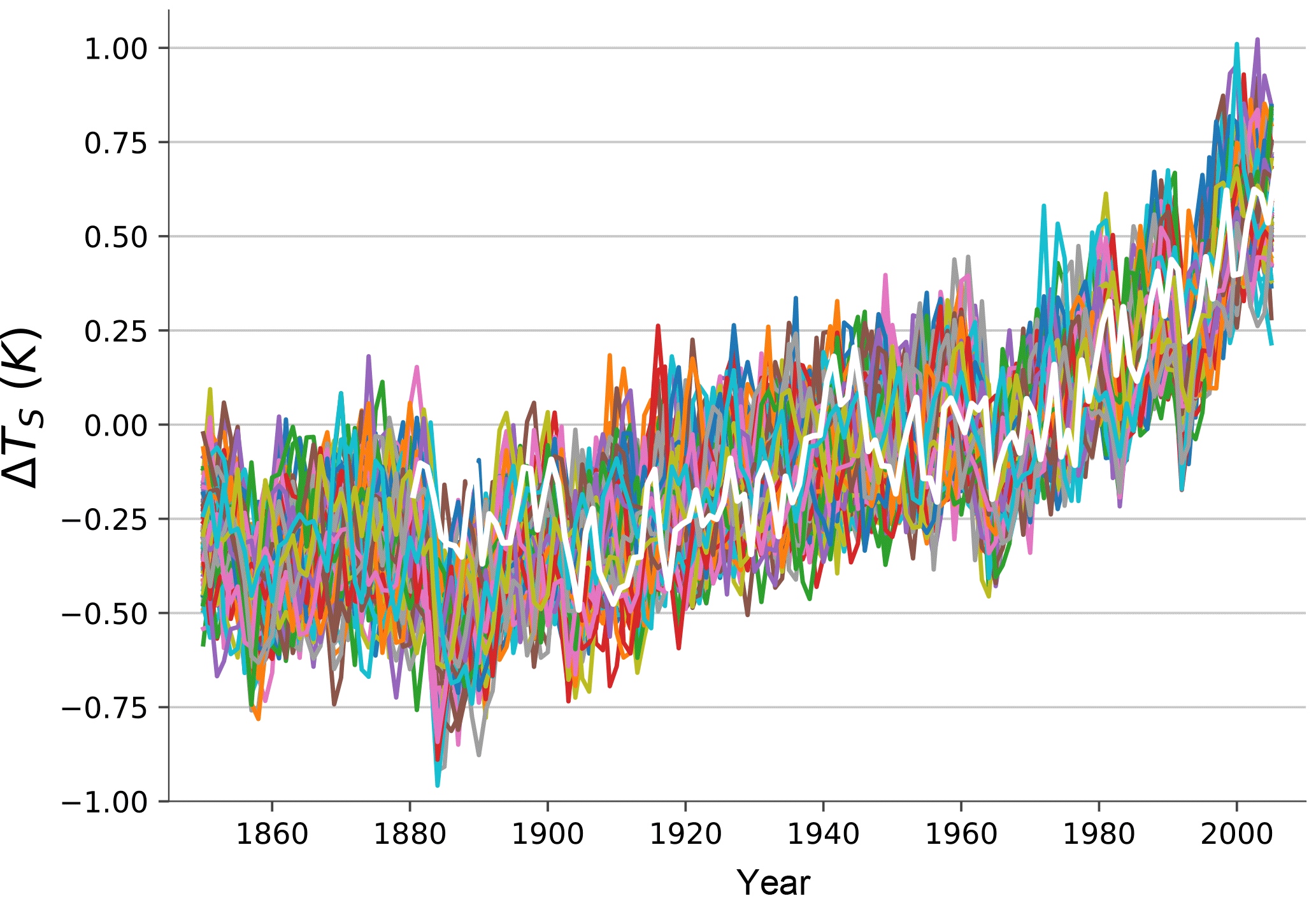
Figure 1Plot of annual and global average surface temperature from the 100 members of the MPI-ESM1.1 ensemble (colored lines), along with the GISTEMP measurements (Hansen et al., 2010) (white line). Temperatures are referenced to the 1951–1980 average.
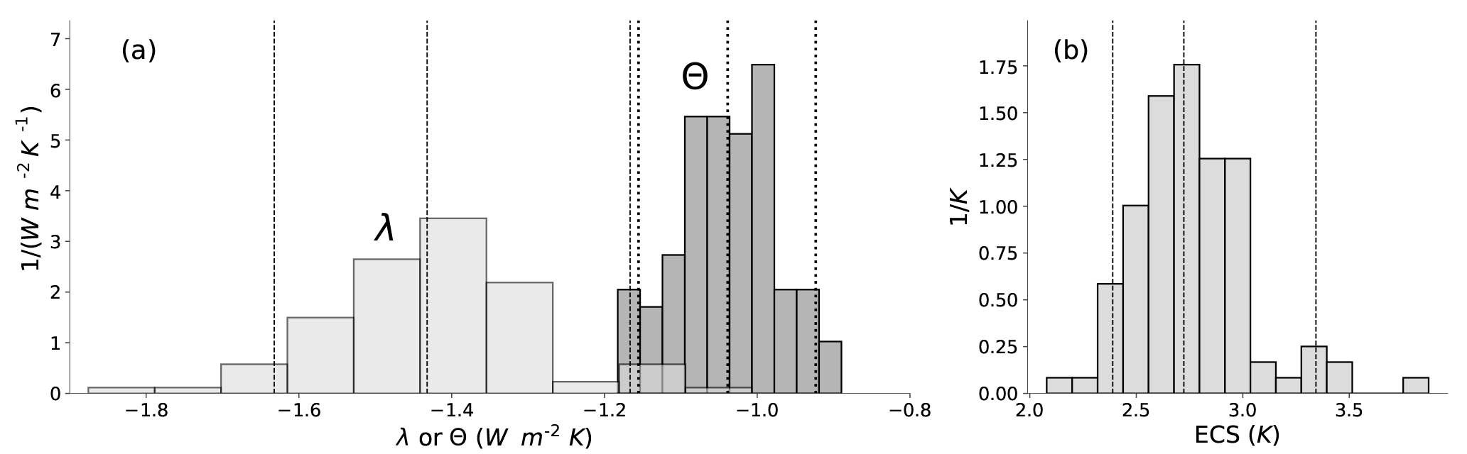
Figure 2Probability density functions (PDFs) of (a) λ (lighter) and Θ (darker) and (b) ECS derived from the members of the MPI-ESM1.1 historical ensemble. The vertical lines are the 5th, 50th, and 95th percentile of each distribution.
We also calculate ECS = for each ensemble member, producing values ranging from 2.08 to 3.87 K (5–95 % range 2.39 to 3.34 K) (Fig. 2b), with an ensemble median of 2.72 K. Thus, our analysis shows that λ and ECS estimated from the historical record can vary widely simply due to internal variability. Given that we have only a single realization of the 20th century, we should not consider estimates based on the historical period to be precise – even with perfect observations. This supports previous work that also emphasized the impact of internal variability on estimates of λ and ECS (Huber et al., 2014; Andrews et al., 2015; Zhou et al., 2016; Gregory and Andrews, 2016).
Previous researchers have questioned whether the historical record provides an accurate measure of λ and ECS, and we can check this by comparing the ensemble values to ECS estimates from a 2×CO2 run of the MPI-ESM1.2, which is physically very close to MPI-ESM1.1. An abrupt 2×CO2 run yields an ECS of 2.93 K in response to an abrupt doubling of CO2 (estimated by regressing years 100–1000 of a 1000-year run) – 8 % larger than the ensemble median. This is in line with the 10 % difference in ECS estimated by Mauritsen and Pincus (2017) to arise from the average CMIP5 model time-dependent feedback but smaller than suggested in other recent studies of ECS in transient climate runs (e.g., Armour, 2017; Proistosescu and Huybers, 2017).
Thus, there are a number of issues that need to be considered when interpreting estimates of λ and ECS derived from the historical period. In addition to the precision and accuracy issues discussed above, it also includes the large and evolving uncertainty in forcing over the 20th century (Forster, 2016), different forcing efficacies of greenhouse gases and aerosols (Shindell, 2014; Kummer and Dessler, 2014), and geographically incomplete or inhomogeneous observations (Richardson et al., 2016).

Figure 3Scatterplot of monthly anomalies of ΔR vs. (a) global average surface temperature ΔTS and (b) tropical average 500 hPa temperature ΔTA. Observations cover the period March 2000–July 2017, and anomalies are deviations from the mean annual cycle. ΔR and temperature time series are detrended to account for forcing. The dashed lines are ordinary least-squares fits; the slope, 5–95 % confidence interval, and correlation coefficient are shown on each panel. Confidence intervals account for autocorrelation of the time series (Santer et al., 2000).
In this section, we explain the physical process by which internal variability leads to the large spread in λ and ECS estimated from the ensemble. We begin by observing that Eqs. (1) and (2) parameterize R−F in terms of global average surface temperature, TS. In model runs with strong forcing driving large warming, such as abrupt 4×CO2 simulations, there is indeed a strong correlation between these variables (e.g., Gregory et al., 2004). However, because R−F in such runs is dominated by a monotonic trend, correlations will exist with any geophysical field that also exhibits a monotonic trend, regardless of whether there is a physical connection between the fields. Thus, one should not take the correlation between R−F and TS in these runs as proving causality.
If TS is a good proxy for the response R−F, we would expect to also see a correlation in measurements dominated by interannual variations. Observational data allow us to test this hypothesis. We use observations of R from the Clouds and the Earth's Radiant Energy System (CERES) Energy Balanced and Filled product (ed. 4) (Loeb et al., 2018), which cover the period March 2000 to July 2017. Our sign convention throughout the paper is that downward fluxes are positive. Temperatures come from the European Centre for Medium-Range Weather Forecasts (ECMWF) Interim Re-Analysis (ERA-Interim) (Dee et al., 2011). We assume forcing changes linearly over this time period and account for it by detrending ΔR and ΔT anomaly time series using a linear least-squares fit to remove the long-term trend.
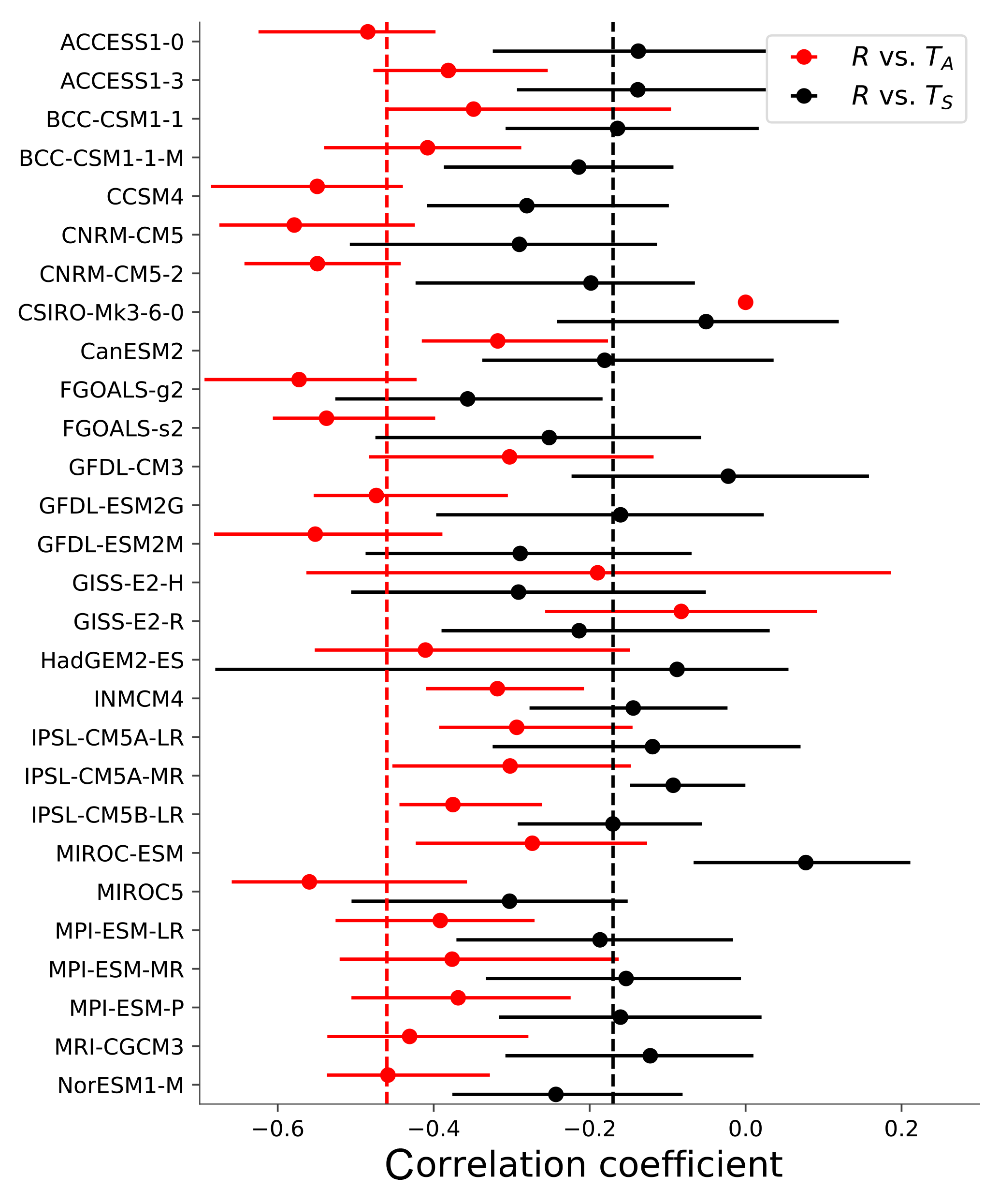
Figure 4Correlation coefficients between ΔR and temperature in CMIP5 control runs: black and red symbols represent the correlation with ΔTS and ΔTA, respectively. The dot is the average of the correlation coefficients from the 17-year segments of the model run; the bars indicate the maximum and minimum values from the control run. The dashed lines are the corresponding correlation coefficients from the CERES regressions in Fig. 3.
These data show that ΔR is poorly correlated with ΔTS in response to interannual variability (Fig. 3a), as has been noted many times in the literature; see, e.g., Sect. 5 of Forster (2016). In particular, the low correlation coefficient tells us that ΔTS explains little of the variance in ΔR. Using explicit estimates of forcing or other temperature data sets (e.g., MERRA-2) yields the same result.
Global climate models that submitted output to CMIP5 (Taylor et al., 2012) also show this poor correlation. To demonstrate this, we have calculated the correlation coefficient between ΔTS and ΔR in CMIP5 pre-industrial control runs (these are runs for which forcing F=0). To facilitate comparison with the CERES data, as well as avoid any issues with long-term drift in the control runs, we break each run into 17-year segments to match the length of the CERES data and calculate the correlation coefficient of monthly anomalies of ΔR and ΔTS for each segment. Figure 4 shows that the correlation between ΔR and ΔTS in the models is similar to that from the CERES analysis.
Recent work provides an explanation: the response of Δ(R−F) to a particular ΔTS is determined not only by the global average magnitude but also by the pattern of warming (Armour et al., 2013; Andrews et al., 2015; Gregory and Andrews, 2016; Zhou et al., 2016, 2017; Andrews and Webb, 2018). During El Niño cycles that dominate the observations in Fig. 3, the spatial pattern of warm and cool regions changes, leading to responses in Δ(R−F) that do not scale cleanly with ΔTS – something Stevens et al. (2016) refer to as “pattern effects”.
To demonstrate how this also generates the spread in λ in the model ensemble (Fig. 2a), we calculate the local response λr in three equal-area regions (90–19.4∘ S, 19.4∘ S–19.4∘ N, 19.4–90∘ N). We define λr as the regional analog to λ (Eq. 2):
where the “r” subscript indicates a regional average value.
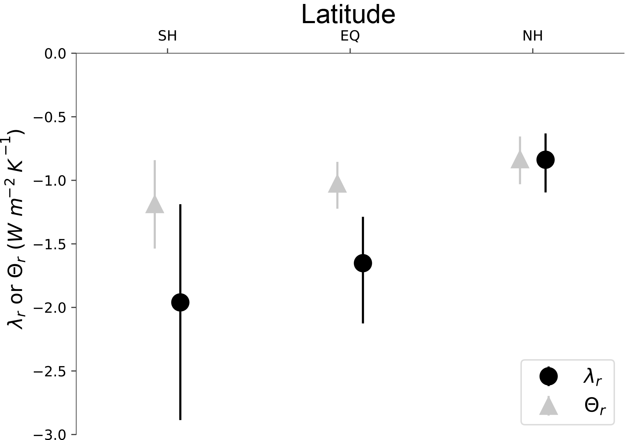
Figure 5λr and Θr calculated as regional average Δ(R−F) divided by regional average temperature (ΔTS for λ and ΔTA for Θ). The regions are 90–19.4∘ S (SH), 19.4∘ S–19.4∘ N (EQ), and 19.4–90∘ N (NH). The values are calculated for each member of the 100-member ensemble; the solid symbols are the ensemble average, while the bars show the 5–95 % range.
We find that λr varies between the regions (Fig. 5). This means that different ensemble members with similar global average ΔTS but different patterns of surface warming produce different values of global average Δ(R−F), thereby leading to spread in the estimated λ among the ensemble members. We also see strong variability in λr within each region, suggesting that how the warming is distributed within the region also drives some of the spread in estimated λ in the ensemble.
This explanation is consistent with analyses showing that λ changes during transient runs as the pattern of surface temperature evolves (Senior and Mitchell, 2000; Armour et al., 2013; Andrews et al., 2015; Gregory and Andrews, 2016; Stevens et al., 2016). In our model ensemble, however, the pattern changes are caused by internal variability rather than differing regional heat capacities that cause some regions to warm more slowly than others during forced warming.
Our analysis demonstrates limitations of the conventional energy balance framework (Eq. 1). It has been previously noted that ΔR correlates better with tropospheric temperatures than ΔTS (Murphy, 2010; Spencer and Braswell, 2010; Trenberth et al., 2015). Other analyses have also stressed the importance of atmospheric temperatures – through its influence on lapse rate – as providing a fundamental control on the planet's energy budget (Zhou et al., 2016; Ceppi and Gregory, 2017). Based on this, we test a new energy balance framework constructed using the temperature of the tropical atmosphere:
where TA is the tropical average (30∘ N–30∘ S) 500 hPa temperature and Θ relates this quantity to R−F. R and F are the same global average quantities they were in Eq. (1). ECS can be expressed in terms of Θ:
where ΔTS and ΔTA are the equilibrium changes in these quantities in response to doubled CO2. The CMIP5 ensemble average ratio ΔTS∕ΔTA is 0.86 ± 0.10 (±1σ), where Δ represents the average difference between the first and last decades of the abrupt 4×CO2 runs.
Support for Eq. (4) can be found in the observations: ΔR shows a tighter correlation with ΔTA than with ΔTS in observations (Fig. 3a vs. Fig. 3b). CMIP5 models also show this (Fig. 4). Given that the slope of these plots can be taken as estimates of Θ and λ, the tighter correlation leads to more accurate estimates of Θ than λ, both in absolute and relative terms.
Turning to the model ensemble, we next demonstrate that Θ is a more precise metric than λ. We do this by calculating Θ [] in each ensemble member, yielding values ranging from −1.18 to −0.89 (5–95 % range −1.16 to −0.92 ), with an ensemble median of −1.04 (Fig. 2a). There is clearly less variability in Θ among the ensemble members than for λ. This reflects less variability in the regional response Θr () than in λr (Fig. 5), as well as less variability within the regions. We therefore conclude that interannual variability has less of an impact on Θ than λ.
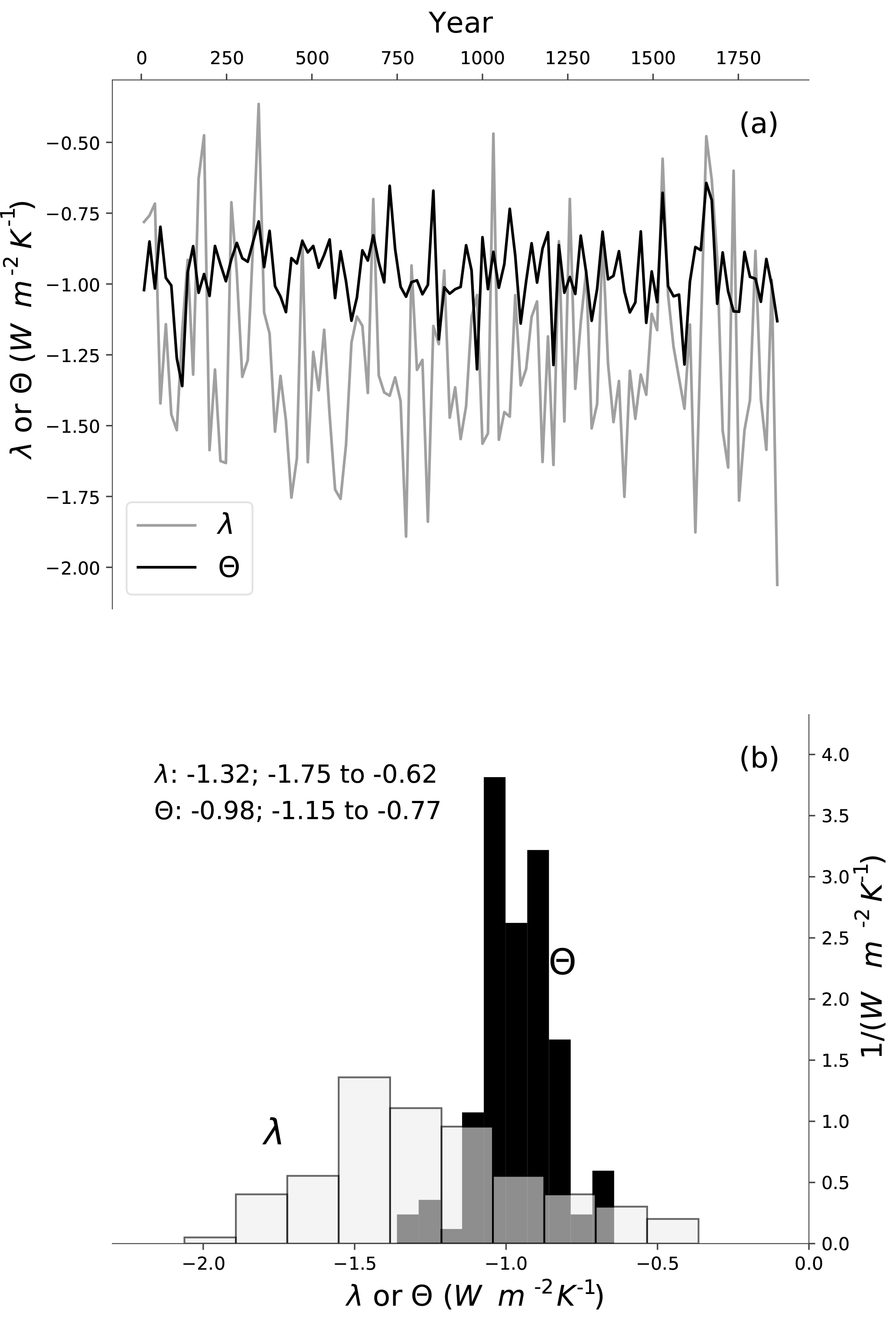
Figure 6(a) Time series of λ (gray) and Θ (black) estimated in a 17-year sliding window of a 2000-year control run of the MPI-ESM1.1. (b) PDFs of the time series in (a). Median and 5–95 % confidence interval for each distribution are displayed on the plot.
We can also reproduce this in a 2000-year control run (a run with fixed pre-industrial boundary conditions) of the MPI-ESM1.1 model. Figure 6 shows λ calculated in a sliding 17-year window and confirms significant temporal variability in λ. We can similarly calculate Θ, and the figure shows that temporal variability in Θ is substantially smaller.

Figure 7The standard deviation (SD) of the λ time series divided by the SD of the Θ time series. Each time series is calculated from 17-year segments of CMIP5 control runs. The dotted line is the ensemble average.
This result is also reproduced in the CMIP5 control models. Figure 7 plots the standard deviation (SD) of each CMIP5 model's set of short-term λ divided by the SD of that model's set of short-term Θ (as described previously, we calculate time series of short-term λ and Θ values for each model by regressing anomalies in a 17-year sliding window of the control runs). All of the models fall above 1, demonstrating that there is less variability in the Θ time series than in the λ time series in every climate model. This confirms that Θ is more robust with respect to internal variability than λ. It also suggests that Θ estimated from the satellite data (Fig. 3) should be considered a better estimate of the climate system's long-term value than λ estimated from the same data set.
As far as accuracy goes, we can compare Θ in the ensemble over the historical period to Θ in response to much larger warming. The ensemble median of Θ from the historic period (Fig. 2), −1.04 ± 0.01 (5–95 % confidence interval), is close to the value obtained from an analysis of the first 150 years of an abrupt 4×CO2 run of the same model, Θ = −1.03 ± 0.04 , as well as Θ calculated from all 2600 years of this run, Θ = −1.00 ± 0.01 (values from the 4×CO2 runs are all obtained using the Gregory method (Gregory et al., 2004) using annual average R and temperatures). On the other hand, λ changes substantially in the 4×CO2 run as the climate warms: λ = −1.36 ± 0.07 when calculated from the first 150 years, but λ = −0.95 ± 0.01 from all 2600 years of that run.
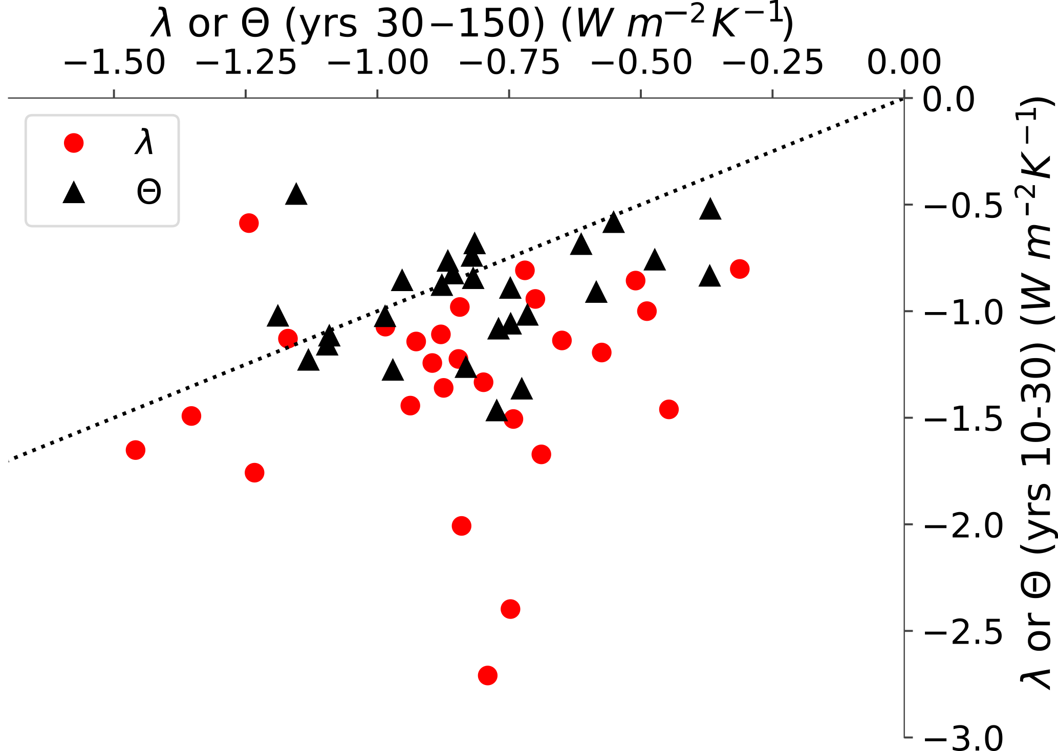
Figure 8Scatterplot of λ10−30 vs. λ30−150 (red circles) in CMIP5 abrupt 4×CO2 runs, as well as Θ10−30 vs. Θ30−150 (black triangles) in the same models. Each point represents one model. The dotted line is the 1:1 line. The subscripts (10–30, 30–150) indicate the years of the run from which the values are calculated.
We can verify this result in the CMIP5 abrupt 4×CO2 ensemble. It has been previously demonstrated that plots of R−F vs. TS do not trace straight lines as the climate warms (Andrews et al., 2015; Rugenstein et al., 2016; Rose and Rayborn, 2016; Armour, 2017), so λ and ECS calculated in a single model run may depend on the portion of the run selected. In the CMIP5 abrupt 4×CO2 ensemble, for example, average λ calculated by regressing years 10–30 (λ10−30) is more negative than λ calculated from years 30–150 (λ30−150) by 0.49 (Fig. 8).
Several explanations for this have been advanced, most prominently that λ is a function of the pattern of surface warming (Senior and Mitchell, 2000; Armour et al., 2013; Andrews et al., 2015; Gregory and Andrews, 2016; Zhou et al., 2016; Stevens et al., 2016). Using Θ largely eliminates this pattern effect: Θ10−30 and Θ30−150 have an average difference of 0.13 for the CMIP5 ensemble (Fig. 8). Thus, we find additional evidence that Θ tends to be similar for different amounts and patterns of warming.
The lack of curvature in the Θ calculations means there is curvature in the relation between TA and TS in the models. Thus, the pattern effect's impact on ECS calculations shifts from λ in the traditional framework to the ΔTS∕ΔTA term in Eq. (4). This also emphasizes the need to improve our understanding of the factors that control ΔTS∕ΔTA, as well as how future patterns of surface warming will evolve.
There are several plausible reasons why TA may control R better than TS. It seems likely that several of the feedbacks – e.g., lapse rate, water vapor, or longwave cloud – should be more strongly influenced by atmospheric temperatures than TS. More recently, it has been shown that atmospheric temperatures also play a key role in regulating low clouds (Zhou et al., 2016, 2017), thereby influencing the shortwave cloud feedback. This is also consistent with Ceppi and Gregory (2017), who identified a dependence of ECS on atmospheric stability in models. We have not further investigated this – ultimately, our use of TA in Eq. (4) is based on observations (Murphy, 2010; Spencer and Braswell, 2010; Trenberth et al., 2015) that it correlates well with R. Other metrics, such as global average atmospheric temperature, work almost as well. Clearly, further investigations on how to best describe the Earth's energy balance are warranted.
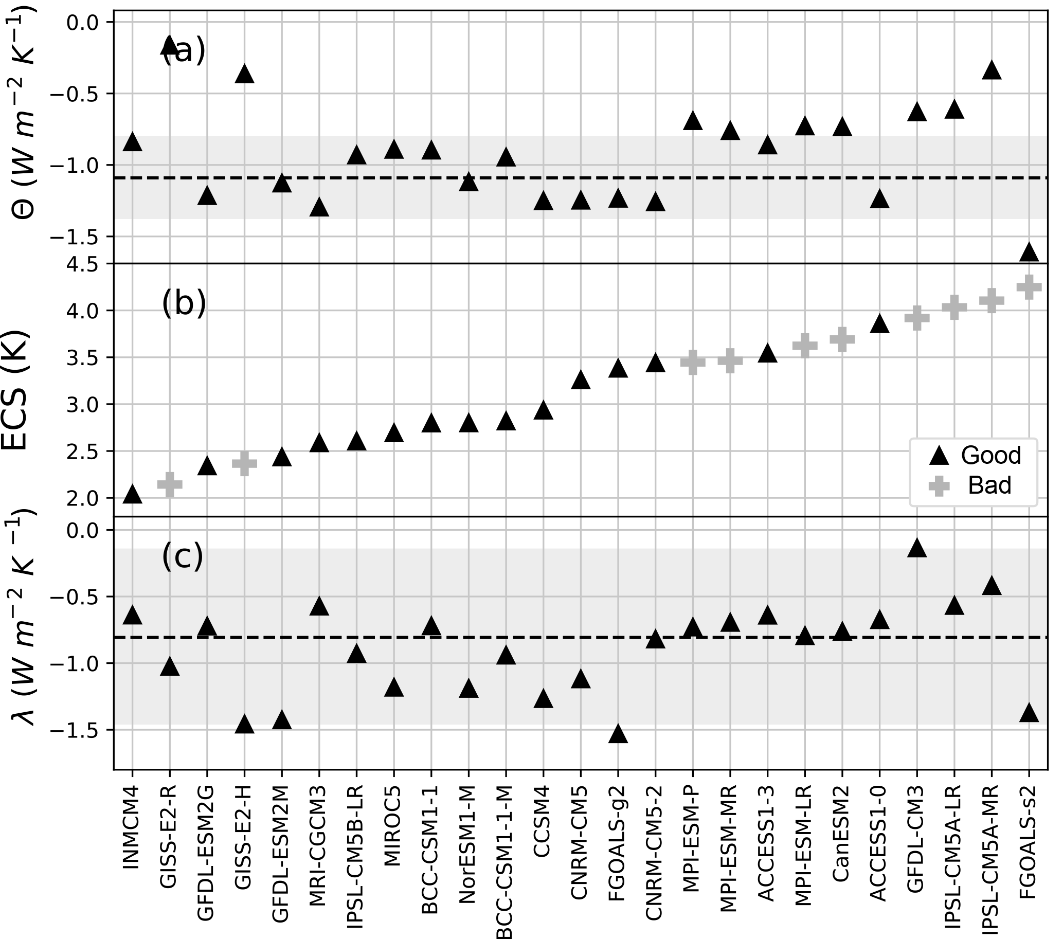
Figure 9(a) Θ from individual CMIP5 control runs. The dotted line is the estimate from CERES observations; the gray region is the 5–95 % confidence band. (b) ECS from each CMIP5 model, estimated from the first 150 years of abrupt 4×CO2 runs using the Gregory method (Gregory et al., 2004). “Good” models are those whose Θ agrees with observations in (a); “bad” models are those whose Θ does not. (c) Same as (a) but for λ.
Finally, one of our ultimate goals for this revised framework is to help produce better estimates of ECS. We are working on a detailed analysis of ECS based on this framework, which is presently in review (Dessler and Forster, 2018), but we briefly show here how the advantages of the revised energy balance framework may be leveraged to do this. Figure 9a shows Θ calculated from control runs of 25 CMIP5 models. To calculate Θ in the control runs, we break each control run into 17-year segments and calculate monthly anomalies of ΔR and ΔTA during each segment. Then, we calculate Θ for each segment as the slope of the regression of ΔR vs. ΔTA for that segment. Thus, for each control run, we generate a large number of estimates of Θ. The value in Fig. 9a is the average of these individual values.
Figure 9b shows the ECS of these models, calculated from the first 150 years of the abrupt 4×CO2 runs using the Gregory method. If we assume that models with more accurate simulation of short-term Θ produce more accurate estimates of ECS (Brown and Caldeira, 2017; Wu and North, 2002), then we can use Fig. 9a and b to constrain ECS. We find that the 15 models whose average short-term Θ falls within the uncertainty of Θ estimated from CERES observations have ECS values ranging from 2.0 to 3.9 K, with an average of 2.9 K. This excludes many of the highest-ECS models, a result consistent with other analyses (Cox et al., 2018; Lewis and Curry, 2015).
It would not have been possible to draw this conclusion with the conventional energy balance framework. Figure 9c shows the comparison between λ from the control runs (calculated the same way Θ was calculated) and CERES observations. Because of the much larger uncertainty in the observational estimate of short-term λ, almost all models fall within the observational range, thereby prohibiting any constraint on the ECS range.
It may also be possible to use the relation between short-term and long-term Θ as an emergent constraint to convert short-term observations to the long-term response. There is some scatter in the relation in the CMIP5 ensemble, however, so more analysis of how these are related is likely required before ECS can be constrained in this way.
We have estimated ECS in each of a 100-member climate model ensemble using the same energy balance constraint used by many investigators to estimate ECS from 20th-century historical observations. We find that the method is imprecise – the estimates of ECS range from 2.1 to 3.9 K (Fig. 2), with some ensemble members far from the model's true value of 2.9 K. Given that we only have a single ensemble of reality, one should recognize that estimates of ECS derived from the historical record may not be a good estimate of our climate system's true value.
The source of the imprecision relates to the construction of the traditional energy balance equation (Eq. 1). In it, the response of TOA net flux (R−F) is parameterized in terms of global average surface temperature (TS). Recent research has suggested that the response is not just determined by the magnitude of TS but also includes other factors, such as the pattern of TS (e.g., Armour et al., 2013; Andrews et al., 2015; Gregory and Andrews, 2016; Zhou et al., 2017) or the lapse rate (e.g., Zhou et al., 2017; Ceppi and Gregory, 2017; Andrews and Webb, 2018). As a result, two ensemble members with the same ΔTS can have different climate responses, Δ(R−F), leading to spread in the inferred λ.
The lack of a direct relationship between TS and radiation balance suggests that it may be profitable to investigate alternative formulations. We test parameterizing the response in terms of 500 hPa tropical temperature (Eq. 4) and find that it is superior in many ways. Ultimately, how investigators describe the energy balance of the planet will depend on the problem and the available data. The surface temperature is indeed special, so the traditional framework may be preferred for some problems. But investigators may find that the alternatives are superior for certain problems, for instance constraining Earth's climate sensitivity.
The data set for the code is availeble at http://dx.doi.org/10.5281/zenodo.1206285, and the data set for the data is available at http://dx.doi.org/10.5281/zenodo.1206267.
The authors declare that they have no conflict of interest.
This work was supported by NSF grant AGS-1661861 to Texas A&M University. This work was initiated while
Andrew E. Dessler was on faculty development leave from Texas A&M during the fall of 2016; he thanks Texas A&M and the
Max-Planck-Institut für Meteorologie for supporting this research. Computational resources were made available by
Deutsches Klimarechenzentrum (DKRZ) through support from German Federal Ministry of Education and Research (BMBF) and by
the Swiss National Supercomputing Centre (CSCS).
The article processing charges for this open-access
publication were covered by the Max Planck Society.
Edited by: Amanda Maycock
Reviewed by: two anonymous referees
Aldrin, M., Holden, M., Guttorp, P., Skeie, R. B., Myhre, G., and Berntsen, T. K.: Bayesian estimation of climate sensitivity based on a simple climate model fitted to observations of hemispheric temperatures and global ocean heat content, Environmetrics, 23, 253–271, https://doi.org/10.1002/env.2140, 2012.
Andrews, T. and Webb, M. J.: The dependence of global cloud and lapse rate feedbacks on the spatial structure of Tropical Pacific warming, J. Climate, 31, 641–654, https://doi.org/10.1175/jcli-d-17-0087.1, 2018.
Andrews, T., Gregory, J. M., and Webb, M. J.: The dependence of radiative forcing and feedback on evolving patterns of surface temperature change in climate models, J. Climate, 28, 1630–1648, https://doi.org/10.1175/JCLI-D-14-00545.1, 2015.
Annan, J. D. and Hargreaves, J. C.: Using multiple observationally-based constraints to estimate climate sensitivity, Geophys. Res. Lett., 33, L06704, https://doi.org/10.1029/2005gl025259, 2006.
Armour, K. C.: Energy budget constraints on climate sensitivity in light of inconstant climate feedbacks, Nat. Clim. Change, 7, 331–335, https://doi.org/10.1038/nclimate3278, 2017.
Armour, K. C., Bitz, C. M., and Roe, G. H.: Time-varying climate sensitivity from regional feedbacks, J. Climate, 26, 4518–4534, https://doi.org/10.1175/jcli-d-12-00544.1, 2013.
Brown, P. T. and Caldeira, K.: Greater future global warming inferred from Earth's recent energy budget, Nature, 552, 45–50, https://doi.org/10.1038/nature24672, 2017.
Ceppi, P. and Gregory, J. M.: Relationship of tropospheric stability to climate sensitivity and Earth's observed radiation budget, P. Natl. Acad. Sci. USA, 114, 13126–13131, https://doi.org/10.1073/pnas.1714308114, 2017.
Collins, M., Knutti, R., Arblaster, J., Dufresne, J.-L., Fichefet, T., Friedlingstein, P., Gao, X., Gutowski, W. J., Johns, T., Krinner, G., Shongwe, W., Tebaldi, C., Weaver, A. J., and Wehner, M.: Long-term climate change: projections, commitments and irreversibility, in: Climate Change 2013: The Physical Science Basis. Contribution of Working Group I to the Fifth Assessment Report of the Intergovernmental Panel on Climate Change, edited by: Stocker, T. F., Qin, D., Plattner, G.-K., Tignor, M., Allen, S. K., Boschung, J., Nauels, A., Xia, Y., Bex, V., and Midgley, P. M., Cambridge University Press, Cambridge, UK and New York, NY, USA, 2013.
Cox, P. M., Huntingford, C., and Williamson, M. S.: Emergent constraint on equilibrium climate sensitivity from global temperature variability, Nature, 553, 319–322, https://doi.org/10.1038/nature25450, 2018.
Dee, D. P., Uppala, S. M., Simmons, A. J., Berrisford, P., Poli, P., Kobayashi, S., Andrae, U., Balmaseda, M. A., Balsamo, G., Bauer, P., Bechtold, P., Beljaars, A. C. M., van de Berg, L., Bidlot, J., Bormann, N., Delsol, C., Dragani, R., Fuentes, M., Geer, A. J., Haimberger, L., Healy, S. B., Hersbach, H., Holm, E. V. Isaksen, L., Kallberg, P., Kohler, M., Matricardi, M., McNally, A. P., Monge-Sanz, B. M., Morcrette, J. J., Park, B. K., Peubey, C., de Rosnay, P., Tavolato, C., Thepaut, J. N., and Vitart, F.: The ERA-Interim reanalysis: configuration and performance of the data assimilation system, Q. J. Roy. Meteorol. Soc., 137, 553–597, https://doi.org/10.1002/qj.828, 2011.
Dessler, A. E. and Forster, P. M.: An Estimate of Equilibrium Climate Sensitivity from Interannual Variability, EarthArXiv, https://doi.org/doi:10.17605/OSF.IO/4ET67, 2018.
Dessler, A. E. and Zelinka, M. D.: Climate feedbacks, in: Encyclopedia of Atmospheric Sciences, edited by: North, G. R., Pyle, J., and Zhang, F., Elsevier, Oxford, 18–25, 2014.
Dessler, M. and Mauritsen, S.: Data sets used to generate the figures, https://doi.org/10.5281/zenodo.1206267, 2018a.
Dessler, M. and Mauritsen, S.: Code to generate figures, https://doi.org/10.5281/zenodo.1206286, 2018b.
Forster, P. M.: Inference of climate sensitivity from analysis of Earth's energy budget, Annu. Rev. Earth Pl. Sc., 44, 85–106, https://doi.org/10.1146/annurev-earth-060614-105156, 2016.
Forster, P. M., Richardson, T., Maycock, A. C., Smith, C. J., Samset, B. H., Myhre, G., Andrews, T., Pincus, R., and Schulz, M.: Recommendations for diagnosing effective radiative forcing from climate models for CMIP6, J. Geophys. Res., 121, 12460–12475, https://doi.org/10.1002/2016jd025320, 2016.
Giorgetta, M. A., Jungclaus, J., Reick, C. H., Legutke, S., Bader, J., Böttinger, M., Brovkin, V., Crueger, T., Esch, M., Fieg, K., Glushak, K., Gayler, V., Haak, H., Hollweg, H.-D., Ilyina, T., Kinne, S., Kornblueh, L., Matei, D., Mauritsen, T., Mikolajewicz, U., Mueller, W., Notz, D., Pithan, F., Raddatz, T., Rast, S., Redler, R., Roeckner, E., Schmidt, H., Schnur, R., Segschneider, J., Six, K. D., Stockhause, M., Timmreck, C., Wegner, J., Widmann, H., Wieners, K.-H., Claussen, M., Marotzke, J., and Stevens, B.: Climate and carbon cycle changes from 1850 to 2100 in MPI-ESM simulations for the Coupled Model Intercomparison Project phase 5, J. Adv. Model. Earth Syst., 5, 572–597, https://doi.org/10.1002/jame.20038, 2013.
Gregory, J. M. and Andrews, T.: Variation in climate sensitivity and feedback parameters during the historical period, Geophys. Res. Lett., 43, 3911–3920, https://doi.org/10.1002/2016GL068406, 2016.
Gregory, J. M., Stouffer, R. J., Raper, S. C. B., Stott, P. A., and Rayner, N. A.: An observationally based estimate of the climate sensitivity, J. Climate, 15, 3117–3121, https://doi.org/10.1175/1520-0442(2002)015<3117:aobeot>2.0.co;2, 2002.
Gregory, J. M., Ingram, W. J., Palmer, M. A., Jones, G. S., Stott, P. A., Thorpe, R. B., Lowe, J. A., Johns, T. C., and Williams, K. D.: A new method for diagnosing radiative forcing and climate sensitivity, Geophys. Res. Lett., 31, L03205, https://doi.org/10.1029/2003gl018747, 2004.
Hansen, J., Sato, M., Ruedy, R., Nazarenko, L., Lacis, A., Schmidt, G. A., Russell, G., Aleinov, I., Bauer, M., Bauer, S., Bell, N., Cairns, B., Canuto, V., Chandler, M., Cheng, Y., Del Genio, A., Faluvegi, G., Fleming, E., Friend, A., Hall, T., Jackman, C., Kelley, M., Kiang, N., Koch, D., Lean, J., Lerner, J., Lo, K., Menon, S., Miller, R., Minnis, P., Novakov, T., Oinas, V., Perlwitz, J.,, Perlwitz, J., Rind, D., Romanou, A., Shindell, D., Stone, P., Sun, S., Tausnev, N., Thresher, D., Wielicki, B., Wong, T., Yao, M., and Zhang, S.: Efficacy of climate forcings, J. Geophys. Res.-Atmos., 110, D18104, https://doi.org/10.1029/2005JD005776, 2005.
Hansen, J., Ruedy, R., Sato, M., and Lo, K.: Global surface temperature change, Rev. Geophys., 48, RG4004, https://doi.org/10.1029/2010rg000345, 2010.
Huber, M., Beyerle, U., and Knutti, R.: Estimating climate sensitivity and future temperature in the presence of natural climate variability, Geophys. Res. Lett., 41, 2086–2092, https://doi.org/10.1002/2013GL058532, 2014.
Kummer, J. R. and Dessler, A. E.: The impact of forcing efficacy on the equilibrium climate sensitivity, Geophys. Res. Lett., 41, 3565–3568, https://doi.org/10.1002/2014gl060046, 2014.
Lewis, N. and Curry, J. A.: The implications for climate sensitivity of AR5 forcing and heat uptake estimates, Clim. Dynam., 45, 1009–1023, https://doi.org/10.1007/s00382-014-2342-y, 2015.
Loeb, N. G., Doelling, D. R., Wang, H., Su, W., Nguyen, C., Corbett, J. G., Liang, L., Mitrescu, C., Rose, F. G., and Kato, S.: Clouds and the Earth's Radiant Energy System (CERES) Energy Balanced and Filled (EBAF) Top-of-Atmosphere (TOA) Edition-4.0 Data Product, J. Climate, 31, 895–918, https://doi.org/10.1175/jcli-d-17-0208.1, 2018.
Mauritsen, T. and Pincus, R.: Committed warming inferred from observations, Nat. Clim. Change, 7, 652–655, https://doi.org/10.1038/nclimate3357, 2017.
Murphy, D. M.: Constraining climate sensitivity with linear fits to outgoing radiation, Geophys. Res. Lett., 37, D17107, https://doi.org/10.1029/2010GL042911, 2010.
Otto, A., Otto, F. E. L., Boucher, O., Church, J., Hegerl, G., Forster, P. M., Gillett, N. P., Gregory, J., Johnson, G. C., Knutti, R., Lewis, N., Lohmann, U., Marotzke, J., Myhre, G., Shindell, D., Stevens, B., and Allen, M. R.: Energy budget constraints on climate response, Nat. Geosci., 6, 415–416, https://doi.org/10.1038/ngeo1836, 2013.
Proistosescu, C. and Huybers, P. J.: Slow climate mode reconciles historical and model-based estimates of climate sensitivity, Sci. Adv., 3, e1602821, https://doi.org/10.1126/sciadv.1602821, 2017.
Richardson, M., Cowtan, K., Hawkins, E., and Stolpe, M. B.: Reconciled climate response estimates from climate models and the energy budget of Earth, Nat. Clim. Change, 6, 931–935, https://doi.org/10.1038/nclimate3066, 2016.
Rose, B. E. J. and Rayborn, L.: The effects of ocean heat uptake on transient climate sensitivity, Curr. Clim. Change Rep., 2, 190–201, https://doi.org/10.1007/s40641-016-0048-4, 2016.
Rugenstein, M. A. A., Caldeira, K., and Knutti, R.: Dependence of global radiative feedbacks on evolving patterns of surface heat fluxes, Geophys. Res. Lett., 43, 9877–9885, https://doi.org/10.1002/2016GL070907, 2016.
Santer, B. D., Wigley, T. M. L., Boyle, J. S., Gaffen, D. J., Hnilo, J. J., Nychka, D., Parker, D. E., and Taylor, K. E.: Statistical significance of trends and trend differences in layer-average atmospheric temperature time series, J. Geophys. Res., 105, 7337–7356, https://doi.org/10.1029/1999jd901105, 2000.
Senior, C. A. and Mitchell, J. F. B.: The time-dependence of climate sensitivity, Geophys. Res. Lett., 27, 2685–2688, https://doi.org/10.1029/2000GL011373, 2000.
Shindell, D. T.: Inhomogeneous forcing and transient climate sensitivity, Nat. Clim. Change, 4, 274, https://doi.org/10.1038/nclimate2136, 2014.
Skeie, R. B., Berntsen, T., Aldrin, M., Holden, M., and Myhre, G.: A lower and more constrained estimate of climate sensitivity using updated observations and detailed radiative forcing time series, Earth Syst. Dynam., 5, 139–175, https://doi.org/10.5194/esd-5-139-2014, 2014.
Spencer, R. W. and Braswell, W. D.: On the diagnosis of radiative feedback in the presence of unknown radiative forcing, J. Geophys. Res., 115, D16109, https://doi.org/10.1029/2009JD013371, 2010.
Stevens, B., Sherwood, S. C., Bony, S., and Webb, M. J.: Prospects for narrowing bounds on Earth's equilibrium climate sensitivity, Earths Future, 4, 512–522, https://doi.org/10.1002/2016EF000376, 2016.
Taylor, K. E., Stouffer, R. J., and Meehl, G. A.: An overview of CMIP5 and the experiment design, B. Am. Meteorol. Soc., 93, 485–498, https://doi.org/10.1175/bams-d-11-00094.1, 2012.
Trenberth, K. E., Zhang, Y., Fasullo, J. T., and Taguchi, S.: Climate variability and relationships between top-of-atmosphere radiation and temperatures on Earth, J. Geophys. Res., 120, 3642–3659, https://doi.org/10.1002/2014JD022887, 2015.
Wu, Q. and North, G. R.: Climate sensitivity and thermal inertia, Geophys. Res. Lett., 29, 1707, https://doi.org/10.1029/2002GL014864, 2002.
Zhou, C., Zelinka, M. D., and Klein, S. A.: Impact of decadal cloud variations on the Earth's energy budget, Nat. Geosci., 9, 871–874, https://doi.org/10.1038/ngeo2828, 2016.
Zhou, C., Zelinka, M. D., and Klein, S. A.: Analyzing the dependence of global cloud feedback on the spatial pattern of sea surface temperature change with a Green's function approach, J. Adv Model. Earth Syst., 9, 2174–2189, https://doi.org/10.1002/2017MS001096, 2017.