2.1 Global model output

The main data used in this analysis are synthetic global EOR fields generated using the Met Office Unified Model in its global NWP configuration. We used the Global Atmosphere 6.0 (GA6) and Global Land 6.0 (GL6) components, described by Walters et al. (2017), with sea surface temperatures and sea ice prescribed from the Operational Sea Surface Temperature and Sea Ice Analysis (Donlon et al., 2012). The sea surface temperatures are updated daily and, therefore, do not exhibit diurnal variability. Operationally, for reasons of computational expense, full radiation calculations are not done every time step (Manners et al., 2009). In GA6, the full radiation calculations are done every hour, with an update to represent the changing cloud fields every 12 min time step (Walters et al., 2017; Manners et al., 2009). In this simulation however, the full radiation scheme, based on Edwards and Slingo (1996), was called on every model time step to better represent the evolution of EOR. The model was run with this set-up for each day from an operational 0000 Z analysis.

The data are provided for each day in September 2010. The year of 2010 was chosen arbitrarily, but the month of September was selected specifically due to the timing of the equinox. At the equinox the day length is approximately constant at all locations on Earth, so the months containing the equinoxes are the only times during the year that a consistent diurnal cycle can be assessed globally. In particular, RSR only has a signature during the daylight hours so away from the equinoxes the analysis would be fundamentally limited in one of the hemispheres. While dominant patterns in the diurnal cycle of EOR do exhibit spatial variations between seasons, the relative importance of physical processes that control the dominant patterns typically remains robust throughout the year (Smith and Rutan, 2003; Rutan et al., 2014). This allows insight to be gained for the entire annual cycle, at least in a qualitative sense, by just considering this unique situation.

The data are provided with a 12 min temporal resolution (i.e. at every model time step) on the N320 grid, giving a spatial resolution of approximately 40 km in mid-latitudes. These temporal and spatial resolutions are selected to retain all relevant information while avoiding data redundancy. This is based on initial experiments in which we reduced the temporal/spatial resolutions artificially in one day of very high resolution ($\mathrm{5}\min /\sim \mathrm{17}$ km in mid-latitudes) global EOR fields, and found that the dominant patterns in the data (see Sect. 3.2) are well retained at a resolution of $\mathrm{15}\min /\sim \mathrm{50}$ km in mid-latitudes.

When analysing the RSR we work with the TOA albedo, similar to Rutan et al. (2014), calculated as the division of outgoing by incoming TOA solar irradiance. This normalization removes the variability associated with the amount of incoming solar radiation that would otherwise dominate the diurnal cycle, but is not of interest here. For September 2010 it is possible to define the TOA albedo from 07:00 to 17:00 local solar time and from 61.5^∘ N to 61.5^∘ S, encompassing over 94 % of the total incoming short-wave irradiance entering the Earth system.

As well as the OLR and TOA albedo, a host of other geophysical variables were simultaneously outputted from the model to aid the physical interpretation of the EOR diurnal cycles. The additional variables included in this study are the equivalent surface and clear-sky radiation fluxes, surface temperature, cloud liquid water path (LWP), cloud ice water path (IWP) and cloud top height (CTH).

2.2 Supporting satellite datasets

Several observational datasets of EOR currently exist that are derived from various satellite instruments. Global EOR observations, such as those from the Clouds and the Earth's Radiant Energy System (CERES) instrument (Wielicki et al., 1996), provide complete coverage but are not used in this study mainly due to their lack of diurnal sampling from low-Earth sun-synchronous orbits. Substantial efforts have been applied to interpolate between the diurnal gaps in CERES sampling (Doelling et al., 2013, 2016) but these products do not match the high temporal resolution of the model data required for thorough investigations of the diurnal cycle. Observations from the Scanner for Radiation Budget (ScaRaB) instrument are capable of capturing long-term averaged diurnal variability due to the drifting orbit of the Megha-Tropiques satellite (Viollier and Raberanto, 2010), but are limited to the central tropics due to the very low inclination of the orbit and are therefore also not appropriate. GERB observations, however, made from the unique vantage point of geostationary orbit, provide EOR at high temporal resolution over a large region including Africa, Europe and their surrounding waters, and are therefore much better suited to this study. An added advantage is that simultaneous retrievals of cloud properties are available from the Spinning Enhanced Visible and InfraRed Imager (SEVIRI) instrument (Schmid, 2000). We therefore choose to use the GERB and SEVIRI observations to support our model analysis.

Specifically, we make use of OLR and TOA albedo observations from GERB 2 (GERB Edition 1 High Resolution (HR) product with “SW combined adjustment” applied) and CTH observations from SEVIRI (Climate Monitoring Satellite Applications Facility (CMSAF) Cloud Property DAtAset using SEVIRI (CLAAS) Edition 2 product, Finkensieper et al., 2016; Benas et al., 2017). We do not include the SEVIRI LWP and IWP products because the retrieval method, which assumes that the cloud phase is the same as the cloud top for the whole column, leads to unphysical diurnal variability during convective cloud development, which turns out to be an important process in the diurnal cycles of both OLR and TOA albedo, as will be shown in Sect. 4. To avoid missing data in the Southern Hemisphere and high uncertainty data near the edge of the field of view (FOV) we use data north of 20^∘ S and with a viewing zenith angle of less than 70^∘, respectively. Unfortunately, the time window of the model and observation data cannot be matched because full diurnal GERB observations are not available close to the equinoxes due to potential instrument damage. Instead we use observations from July 2006. This month accommodates large solar insolation over the Northern Hemisphere land mass in the GERB FOV that should amplify any diurnal signatures in these regions, and was also the subject of the Comer et al. (2007) study. We acknowledge that it would be ideal to use model output from July 2006 for comparison with these observations. However, to fully capitalize on understanding the diurnal cycle at a global scale, it is crucial to use the model output for September because the relative importance of processes inferred from a global and a regional scale can be quite different (as discussed in Sect. 4.1).

Note that the longitudinal coverage of GERB has recently been extended to include the Indian Ocean (Dewitte et al., 2017), but the coverage remains well short of global. This lack of global coverage removes the opportunity to investigate processes across regions that is afforded by the model data, but at least allows us to evaluate our model results over one portion of the globe. The potential for global diurnal sampling of EOR from a single observing system has recently been highlighted via the use of a constellation of small satellites (Gristey et al., 2017) but, for now at least, observations required to resolve the diurnal cycle fully in global EOR do not exist.

3.1 Pre-processing

Before performing PCA, we must ensure that the data fields are in an appropriate format for extracting patterns of diurnal variability. This involves conversion of the diurnal time coordinate, creation of an average diurnal cycle and a correction to account for changes in grid resolution, implemented as follows.

First, all data fields are transformed from UTC to local solar time. This is required such that all spatial locations correspond to the same part of the diurnal cycle. To achieve this transform, we note that each longitude column in UTC represents a single local solar time. We then select the longitude columns from each UTC map that correspond to the same local solar time and combine them to generate a new set of maps that are now a function of local solar time.

Next, we calculate the monthly average diurnal cycle for each data field by simply averaging the local solar time maps from each day in the month. Since the variations on any given day consist of not only diurnal variations, resulting from the periodic forcing, but also transient weather variations, which are not diurnally forced, performing this monthly averaging helps to reduce the noise from weather events and extract the signal from the diurnal variations of interest.

Lastly, since the data are on equal latitude–longitude grids, we apply a latitude correction by multiplying each grid point by the square root of the cosine of its latitude. This avoids spurious poleward enhancement of variability due to the changes in grid spacing (e.g. Wallace et al., 1992; Comer et al., 2007; Bakalian et al., 2010).

Note that we do not separate data over ocean and land before performing PCA. This is because we intend to reveal global patterns and their relative importance across all regions. Comer et al. (2007) showed that the behaviour of the system can be captured well by considering the diurnal cycles over ocean and land simultaneously.

3.2 Extracting dominant patterns of EOR diurnal variability

PCA applied to the local solar time, monthly averaged and latitude-corrected fields of OLR and TOA albedo extracts empirical orthogonal functions (EOFs) and principal components (PCs) that reveal spatial and temporal patterns in the data, respectively. The first PC describes the maximum possible variance, and each subsequent PC describes the maximum possible variance remaining once the preceding PCs have been removed. There are several approaches to achieve PCA. The approach used in this study is outlined below.

First, we generate a data matrix, F, containing the spatial–temporal data to be used as input for the PCA. The matrix F has t rows and s columns, where t is the number of time steps in the diurnal cycle and s is the total number of spatial grid points. In other words, each row of F consists of a flattened map of the data field at a given local solar time, and each column represents a time series at a given location. Additionally, the mean is removed from each column of F to give an anomaly time series.

In a standard PCA one would next form the large covariance matrix, R, of F given by

and perform an eigenvalue decomposition on R to obtain the EOFs. However, in this application F is very non-square (the spatial dimension is much greater than the temporal dimension), which would result in a very large s×s covariance matrix from Eq. (1) and an expensive eigenvalue decomposition. To reduce computational expense, we follow the equivalent method to obtain the leading EOFs and PCs by forming the smaller t×t covariance matrix, R^∗, given by

The eigenvalue problem for the small covariance matrix, R^∗, in Eq. (2) is formulated as

where C^∗ is a t×t matrix with columns comprising the eigenvectors of R^∗ ; and λ^′ is a t×t diagonal matrix containing the corresponding eigenvalues in descending order. For convenience, the diagonal elements of λ^′ are placed into λ, a row vector of length t.

The eigenvalues, λ, from Eq. (3) are also the leading eigenvalues of the large covariance matrix, R, in Eq. (1). However, the leading eigenvectors of R are not C^∗, but are represented by columns in a s×t matrix C. These column vectors, C_j, are calculated as

A proof of this relationship is provided by Bjornsson and Venegas (1997). The column vectors C_j are the EOFs that we seek. For illustrative purposes, we scale each EOF such that the maximum absolute value is 10.

The corresponding PC is calculated by projecting the original data matrix, F, on to the EOF, C_j, in Eq. (4) as

where A_j, a column vector of length t, is the PC that we seek.

The percentage variance, τ_j, explained by the EOF/PC pair from Eqs. (4) and (5) is

3.3 Coupling dominant patterns of diurnal variability

To aid physical interpretation of the leading EOR EOFs, the corresponding PCs and the percentage variance they explain, respectively calculated from Eqs. (4)–(6), we also investigate their extent of coupling with the variability in other geophysical variables. Coupled PCA patterns between multiple variables have been widely examined in the weather and climate sciences (e.g. Kutzbach, 1967; Wallace et al., 1992; Deser and Blackmon, 1993; Zhang and Liu, 1999) but this additional step has not been applied in previous PCA studies of EOR.

A comprehensive overview of the advantages and disadvantages of common techniques used to identify coupled patterns is given by Bretherton et al. (1992). Here, we are interested in the relationship between a selected pattern of variability in EOR and all of the variability in another variable, which is well suited to an analysis technique previously referred to as single-field PCA (e.g. Wallace et al., 1992). In our application, this will involve studying the correlations between a PC in either OLR or TOA albedo with the diurnal cycle of another variable that we expect to be related to the PC. These correlations are illustrated as heterogeneous correlation maps, which reveal the spatial distributions of where the selected EOR PC has the highest correlations with the diurnal variability in the other variable.

Before generating the heterogeneous correlation maps, we first perform a cross-correlation between the selected EOR PC and the related PC of the other variable to identify any lag between the patterns. Both PCs represent global time series with the rationale that the radiation PC is dominated by a certain process, and the other PC exhibits variability directly related to that process. The cross-correlation is achieved here by calculating a set of Pearson correlation coefficients between the PC of the other variable, which remains fixed in time, and the EOR PC, which is shifted by one time step at a time throughout the entire diurnal cycle. For the TOA albedo, the correlation coefficients are calculated for the time window over which it is defined. From this cross-correlation we can extract the maximum correlation coefficient magnitude, giving an indication of the strength of coupling, and the lag time at which it occurs, giving an indication of how out of phase the patterns are. We define the lag time to be positive when the PC of EOR follows the PC of the other variable (e.g. a change in OLR occurs after the development of LWP). The lag time is then removed before calculating the heterogeneous correlation maps.

The lag times themselves also provide insight into processes and their evolution. We therefore calculate the lag times between various radiation and cloud variables in both the model and GERB/SEVIRI observations. Since the observational data are provided on an irregular grid, we linearly interpolate the observational data onto the same grid as the model data in order to perform the local solar time conversion (see Sect. 3.1).

4.1 Dominant patterns of diurnal variability in modelled global OLR

The first EOF of the global OLR diurnal cycle (Fig. 1a) reveals positive weights, indicating a consistent sign in the diurnal variations, over land surfaces that are largest in arid regions such as the Sahara Desert, Atacama Desert and Arabian Peninsula. The corresponding PC (Fig. 1c) reaches maximum amplitude just after local midday and minimum amplitude overnight. This spatio-temporal pattern is consistent with that expected from solar heating of the land surface and accounts for 68.5 % of the global diurnal variance.

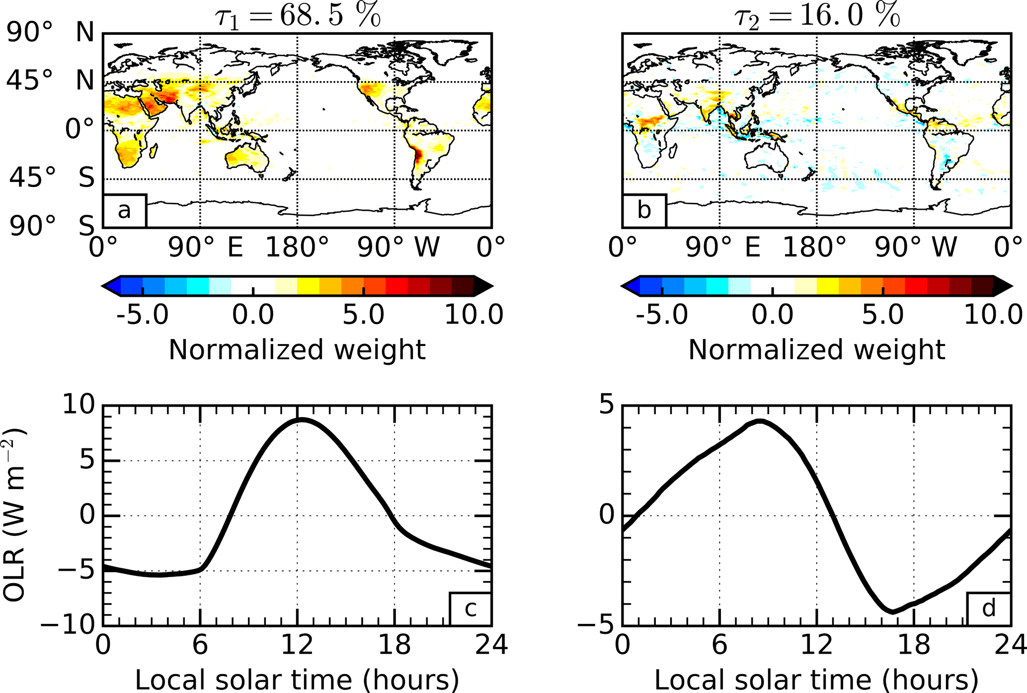
Figure 1Principal component analysis of the global outgoing long-wave radiation (OLR) diurnal cycle for September 2010 in the Met Office model. The empirical orthogonal functions (a and b) and principal components (c and d) are presented for the first (a and c) and second (b and d) most dominant patterns of variability. The percentage variance explained by each pattern is stated above the corresponding empirical orthogonal function.

Download

Although solar heating occurs primarily at the surface, the atmosphere is also heated mainly via absorption of the increased surface emission. The OLR can therefore increase due to increased emission from the warmer atmosphere, as well as increased emission from the warmer surface. To understand whether the first diurnal pattern of OLR (Fig. 1a and c) is dominated by surface or atmospheric heating, we performed the following radiative transfer calculations, and use the Sahara Desert as an example since this region contributes strongly to the diurnal pattern.

Firstly, for a surface emission change of ΔSE due to an increased surface temperature, the atmospheric transmittance, Tr, can be derived as

where ΔOLR is the corresponding change in OLR. Assuming an increase of 1 K in surface temperature, Fig. 2a shows that Tr ranges between 15 and 38 % in various clear-sky conditions, larger than the global mean of 10 % reported by Costa and Shine (2012) for all-sky conditions. Since the dry and predominantly clear-sky atmosphere over the Sahara Desert corresponds to a similar amount of water vapour to that of the mid-latitude winter profile used in Fig. 2a, we take 30 % as an estimate for Tr in the next back-of-the-envelope calculations.

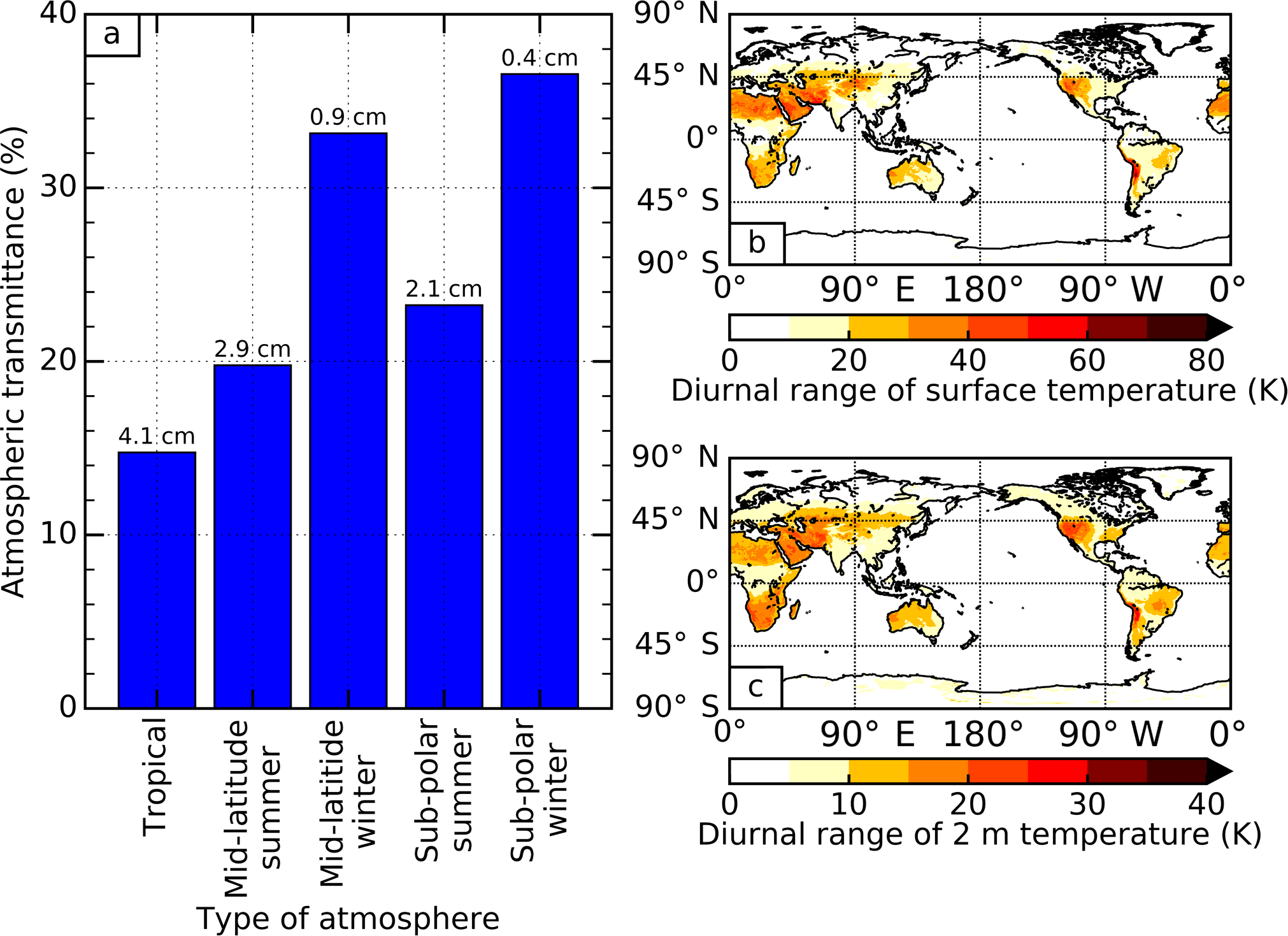
Figure 2(a) Atmospheric transmittance calculated from radiative transfer, using standard atmospheric profiles with various amounts of precipitable water (denoted above each bar). Panels (b) and (c) show the maps of diurnal range of surface temperature and 2 m temperature, respectively, calculated from the average diurnal cycle for September 2010 in the Met Office model. The transmittance is calculated using Eq. (7), given as a ratio of changes in outgoing long-wave radiation to changes in surface emission, assuming a 1 K increase in surface temperature. The initial surface temperatures used in calculations are 299.2 K (tropical profile), 285.8 K (mid-latitude summer and winter profiles) and 256.4 K (sub-polar summer and winter profiles), calculated by averaging modelled surface temperature over the regions of 30^∘ N–30^∘ S, 30–60^∘ N and S and 60–90^∘ N and S, respectively. The Discrete Ordinate Radiative Transfer (DISORT) model Santa Barbara DISORT Atmospheric Radiative Transfer (Ricchiazzi et al., 1998) is used here.

Download

Now we estimate ΔSE in Eq. (7) for the Sahara Desert region from model output. Figure 2b shows that the model diurnal surface temperature range in the Sahara Desert is around 40 K, with a typical minimum surface temperature of 293 K at night-time and a maximum surface temperature of 333 K at daytime. This diurnal temperature change leads to a ΔSE of ∼250 W m⁻², assuming a surface emissivity of 0.9 over the Sahara Desert (Ogawa and Schmugge, 2004). Combining the estimated Tr of 30 %, from Eq. (7) we can derive ΔOLR to be ∼75 W m⁻². This is comparable to the magnitude of the total change represented by the combination of the first EOF and PC (Fig. 1a and c), without considering any change in atmospheric temperature.

Similarly to the previous exercise, we next consider the case of fixed surface temperature and instead perturb the atmospheric temperature. Figure 2c shows that the diurnal range of atmospheric temperature close to the surface (2 m altitude) is already a factor of 2 smaller than at the surface itself. By examining some vertical profiles of diurnal temperature range in the Sahara Desert (not shown), we find that the diurnal temperature range becomes negligible at around 100 m altitude. Taking an exaggerated case that the magnitude of the 2 m diurnal temperature range, ∼20 K in the Sahara Desert, is present over the entire bottom 100 m of the atmosphere, and fixing the surface temperature at the centre of the diurnal range of 313 K, results in ΔOLR of less than 1 W m⁻² for the mid-latitude winter atmosphere. This result holds regardless of whether the initial atmospheric temperature is taken from the standard mid-latitude winter atmosphere, or from the September 2010 minimum and maximum 2 m model temperatures in the Sahara Desert, and is consistent with the fact that the atmosphere is an order of magnitude less efficient at increasing OLR for a given change in temperature (Soden et al., 2008). We therefore conclude that the first spatial–temporal pattern in the diurnal cycle of OLR is dominated by increased surface emission.

The second EOF (Fig. 1b) contains consistent features across many different regions, but the features themselves are small in spatial extent and therefore difficult to interpret at the global scale. When examining the Maritime Continent region as an example (Fig. 3), we find positive weights over the islands that are enhanced along the coastlines and negative weights just offshore. Similar patterns are seen in other coastal regions in the tropics. The corresponding PC (Fig. 1d) shows that these patterns are at a minimum in the late afternoon and a maximum in the early morning. This spatio-temporal pattern, accounting for 16.0 % of the global diurnal variance, is consistent with the OLR signature from the cold tops of deep convective clouds that develop over land during the late afternoon and over the oceans in the early morning. The unique topography of this region permits strong sea breezes (Qian, 2008), explaining the enhancement along the coastlines. Note that in the studies by Smith and Rutan (2003) and Rutan et al. (2014), coastal data are omitted. The spatial patterns of OLR in this region also match surprisingly well with retrieved rainfall at different times during the diurnal cycle, as presented by Love et al. (2011) using observations from the Tropical Rainfall Measuring Mission (TRMM). However, the timing of the minimum modelled OLR signal is substantially earlier than the peak in TRMM retrieved rainfall, consistent with well documented model biases in the timing of convection (e.g. Yang and Slingo, 2001).

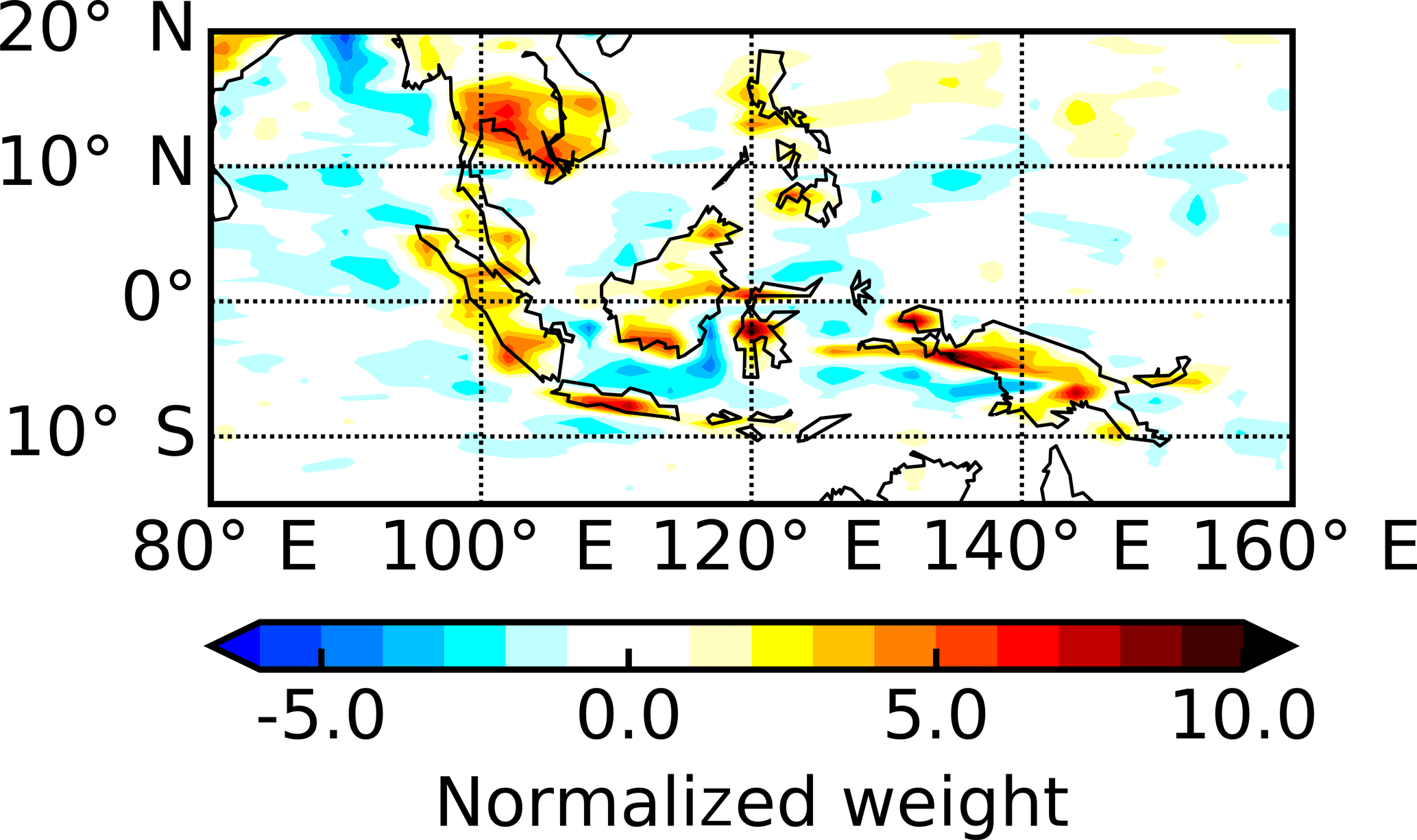
Figure 3A zoom-in of Fig. 1b showing the second empirical orthogonal function over the Maritime Continent region bounded by 15^∘ S–20^∘ N and 80–160^∘ E.

Download

Both of the dominant EOFs and PCs of OLR diurnal variability in Fig. 1 are, reassuringly, similar to those identified with GERB (Comer et al., 2007) and ERBS (Smith and Rutan, 2003) observations, despite the different regions and time periods considered. However, what is markedly different is the percentage variance that these patterns account for. Comer et al. (2007) considered the domain of analysis as a whole rather than separating land and ocean, facilitating a direct comparison with our results. The variances explained by the dominant patterns in their study were 82.3 and 12.8 %. To first order, this suggests that their results exhibit a higher relative contribution from surface heating to the OLR diurnal variability and a lower relative contribution from convective processes, although there may also be an influence from the fact that the actual diurnal variations in some regions can be better explained by a contribution from both dominant patterns for reasons such as surface thermal lag (Futyan and Russell, 2005). This only appears to be the case for a small number of regions including the Tibetan Plateau and parts of southern Africa. However, the total variance explained by their first two patterns is higher at 95.1 % compared with 84.5 % in our results. These differences could be a result of the different time periods and spatial regions considered, or model–observation discrepancies such as the fixed sea surface temperatures in the model. To isolate the influence from different spatial regions, we repeated our analysis using the model data subsampled over the GERB FOV (not shown), and found that the total variance explained by the first two patterns increases to 89.6 %, indicating that around half of the difference is due to the disproportionately high fraction of land mass within the GERB FOV. This is because the first two dominant patterns of OLR diurnal variability appear to be driven, directly and indirectly, by solar heating of land mass. Interestingly, this suggests that the relative importance of diurnal processes acting within the GERB FOV, the only portion of the Earth for which we currently make well resolved diurnal observations of EOR, may not be representative of the global OLR diurnal cycle.

4.2 Dominant patterns of diurnal variability in TOA albedo

4.2.1 From model output

PCA is repeated for the TOA albedo diurnal cycle. The dominant pattern of variability, explaining 88.4 % of the total variance, consists of an EOF (Fig. 4a) with positive weights everywhere, and a diurnally symmetric PC (Fig. 4c) that follows the inverse timing of incoming short-wave irradiance. The dominance of this leading spatio-temporal pattern, despite being consistent with observations from the ERBS (Rutan et al., 2014), is somewhat surprising given that the TOA albedo is a quantity normalized by the amount of incoming solar radiation. This dominance indicates a strong dependence of the TOA albedo on the SZA itself that has been well documented in empirically based angular distribution models (Loeb et al., 2003, 2005; Su et al., 2015), but warrants further investigation into the physical processes at play.

Figure 4Same as Fig. 1, but for the top-of-atmosphere (TOA) albedo.

Download

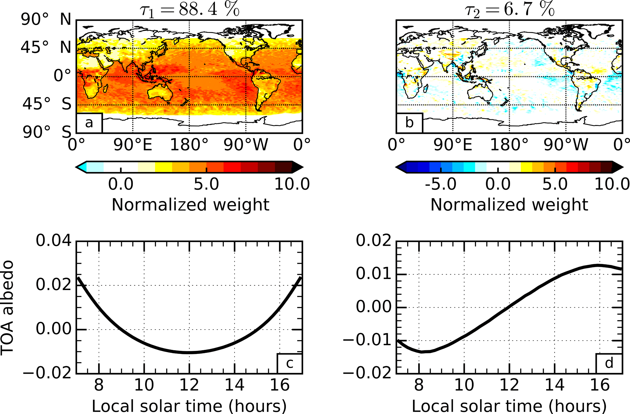
The first PC in Fig. 4c has a U-shape feature, representing a dependence on 1∕μ₀, where μ₀ is the cosine of SZA. To illustrate how the cloud-free atmosphere contributes to the shape, Fig. 5 shows TOA albedos from offline radiative transfer simulations under various simplified situations. For a typical example of an aerosol-free atmosphere, we see that Rayleigh scattering dominates and that atmospheric absorption is only able to counteract this dependence when the Rayleigh scattering is scaled down to around 10 % of its original value (Fig. 5a). Adding a moderate amount of aerosol into the simulations (Fig. 5b), we find that the U shape is retained but is scaled to a different magnitude. In fact, this U shape is not limited to certain atmosphere set-ups or aerosol types because, in low optical depth atmospheres, different optical depths, single scattering albedos and asymmetry parameters only provide a scaling of the shape. In other words, the reflectance function of the atmosphere under a single-scattering approximation always retains a dependence on 1∕μ₀ since this is the factor by which the path length increases and heightens the chance of a scattering event occurring. As a result, the first EOF (Fig. 4a) exhibits weakly positive weights in many different predominantly cloud-free regions, such as the global deserts.

Figure 5Simulation of top-of-atmosphere (TOA) albedo as a function of solar zenith angle (SZA). The dashed lines (a) represent atmospheres where a scaling factor has been applied to the Rayleigh scattering (RS). The dotted lines (b) represent atmospheres where either aerosols are included, or the surface albedo is set to zero (black surf.), or both. The solid red line with star marker appearing in both plots represents the standard atmosphere (Stnd. atm.) with no modifications. All simulations assume a US62 standard atmosphere over a Lambertian vegetated surface unless otherwise stated. When aerosols are included, their optical depth is set to 1 at 550 nm and their optical properties are typical of rural aerosols. Details of the aerosol optical properties and the tool used to perform these calculations, the Discrete Ordinate Radiative Transfer (DISORT) model Santa Barbara DISORT Atmospheric Radiative Transfer, are given by Ricchiazzi et al. (1998).

Download

The influence of the surface and cloud is also clearly evident in the first EOF. There are generally larger weights over the ocean than the land, and the largest weights occur in regions of persistent cloud (e.g. marine stratocumulus regions and the intertropical convergence zone (ITCZ)). The larger diurnal variations over the oceans can be seen by comparing the global-mean diurnal cycle of TOA albedo separated over land and ocean explicitly (Fig. 6a). The reason for these differences is revealed by examining the diurnal cycle in the albedo defined at the surface (Fig. 6b); we find the albedo over land surfaces is larger and diurnally constant. The erosion of the U shape by brighter surfaces can be seen in Fig. 5b, and the SZA dependence of the surface albedo itself follows directly from the set-up of surface albedo in the model, which is Lambertian over land, but uses a modified version of the parametrization from Barker and Li (1995) over the ocean. Similarly, the larger diurnal variations in the presence of cloud can be seen by comparing the global-mean diurnal cycles of all-sky (Fig. 6a) and clear-sky (Fig. 6c) TOA albedo. The differences are particularly evident over land, where the diurnal range in global mean albedo reduces from 0.11 in the all-sky field to 0.07 in the clear-sky field. This is consistent with the sharp contrast in the EOF over land (Fig. 4a) between predominantly cloudy regions, such as along the ITCZ over central Africa, and predominantly clear-sky regions, such as immediately north of the ITCZ over Africa. Note that the U shape can also become weaker as the mean cloudiness of a region increases because the amount of radiation scattered to space per unit optical depth decreases with increasing cloud optical depth. Over both land and ocean surfaces, cloud introduces a more rapid change in the TOA albedo close to midday when the incoming solar radiation is most intense.

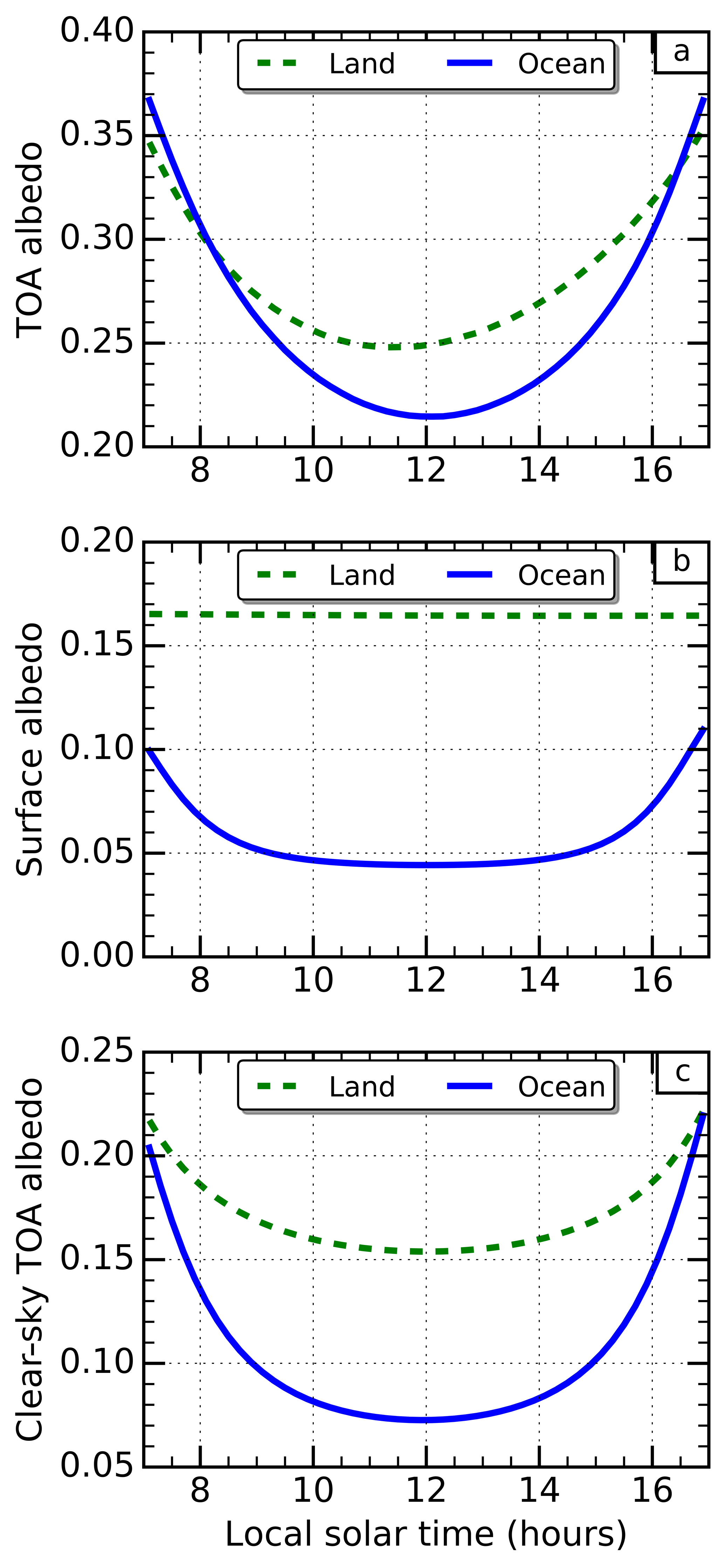
Figure 6The diurnal cycle of global mean albedo for September 2010 in the Met Office model for (a) top-of-atmosphere (TOA) all-sky, (b) surface and (c) TOA clear-sky albedo, separated over land (green dashed line) and ocean (blue solid line).

Download

The second EOF of the TOA albedo diurnal cycle (Fig. 4b) contains many smaller scale features similar to those of the second EOF for OLR. In fact, zooming in to the Maritime Continent region again (Fig. 7) reveals very similar patterns. The corresponding PC (Fig. 4d), however, is reversed in sign when compared with the second PC for OLR. This is consistent with the enhanced reflection from convective clouds that develop over land during the late afternoon and over the oceans in the early morning. This acts to skew the TOA albedo diurnal cycle to earlier in the day over land (minimum around 11:20 local solar time) and later in the day over the oceans (minimum around 12:10), which is evident in Fig. 6a. This spatio-temporal pattern explains just 6.7 % of the total variance.

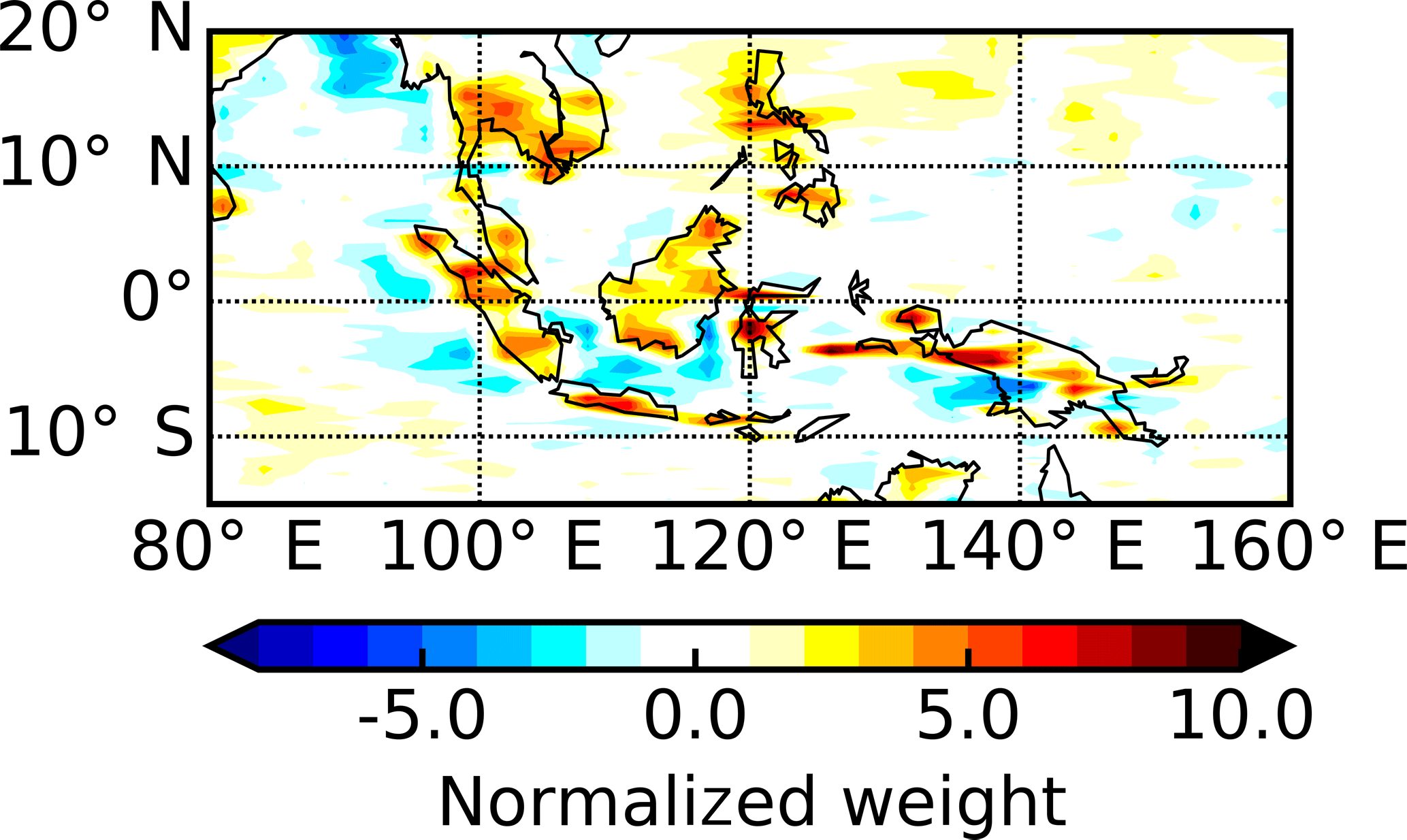
Figure 7A zoom-in of Fig. 4b showing the second empirical orthogonal function over the Maritime Continent region bounded by 15^∘ S–20^∘ N and 80–160^∘ E.

Download

Although the patterns in the second EOFs of TOA albedo and OLR are remarkably similar in the Maritime Continent region, there are obvious differences in other regions. In particular, the marine stratocumulus regions located to the west of continental land masses exhibit negative weights in the TOA albedo EOF that do not appear in the OLR EOF. This signal appears to be related to the diurnal development and dissipation of marine stratocumulus clouds themselves, and is not apparent in the OLR since these variations occur close to the surface. The diurnal cycle of these clouds has been well characterized by ship track observations (Burleyson et al., 2013) and more extensive field campaigns (Boutle and Abel, 2012) as having a maximum thickness overnight/during the morning and a minimum thickness during the afternoon/evening induced by solar absorption of the cloud layer, a process that is relatively well represented in weather and climate models (Pfeifroth et al., 2012) and which appears to be captured by the model here. The fact that the diurnal cycles of convective cloud (e.g. in the Maritime Continent region) and marine stratocumulus cloud (e.g. to the west of continental land masses) are present in the same pattern of variability is noteworthy in itself. Their opposite sign suggests that they are leading to compensating effects: the enhanced reflection from the development of convective cloud in the afternoon is compensated by the reduced reflection from dissipating marine stratocumulus cloud.

4.2.2 From GERB observations

Finally, we present a PCA of TOA albedo using GERB observations (Fig. 8) and compare it with results from the model data, noting that the modelled patterns are similar when subsampled over the GERB FOV (not shown). The leading pattern of variability remains very dominant, explaining 79.5 % of the variance. The first EOF (Fig. 8a) matches the patterns in the model data well, repeating the larger positive weights over the ocean, the south-east Atlantic marine stratocumulus region and equatorial Africa. The northward migration of the ITCZ between September (model fields) and July (GERB observations) is evident over Africa. The first PC (Fig. 8c) also matches the model's diurnally symmetric timing of this pattern associated with the SZA dependence.

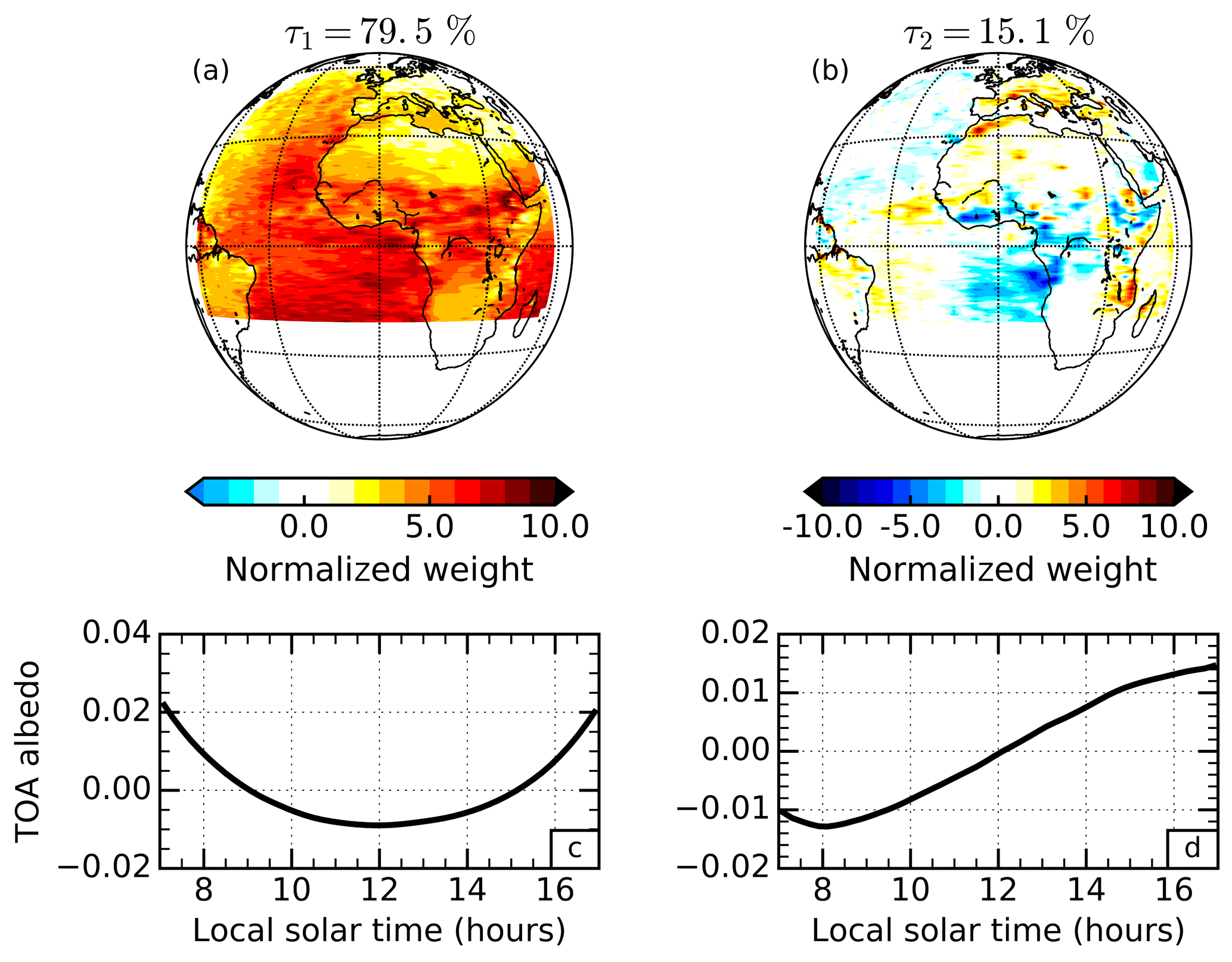
Figure 8Principal component analysis of the top-of-atmosphere (TOA) albedo diurnal cycle for July 2006 in observations from the Geostationary Earth Radiation Budget instrument. The empirical orthogonal functions (a and b) and principal components (c and d) are presented for the first (a and c) and second (b and d) most dominant patterns of variability. The percentage variance explained by each mode is stated above the corresponding empirical orthogonal function.

Download

The second pattern of variability, explaining 15.1 % of the variance, consists of an EOF (Fig. 8b) that contains similar features to those in the second EOF of OLR in the study by Comer et al. (2007) attributed to convective cloud development. However, just like the equivalent model EOF, this EOF also contains negative weights around the west coast of southern and central Africa and the south-east Atlantic related to the diurnal cycle of marine stratocumulus cloud. These patterns provide observational support that the compensating influences of convective and marine boundary layer cloud evolution on the TOA albedo are robust. The positive peak of the second PC (Fig. 8d), however, is shifted to slightly later in the day compared with the model results. The later timing of peak convection in reality compared to the model could be what is pulling the observational PC to later in the day, but the marine stratocumulus variations appear to follow the shift as well, suggesting that the stratocumulus could also be breaking up too early in the model. Unrealistic breaking up of marine stratocumulus in the Met Office model has been previously documented by Allan et al. (2007). One consequence of this shift is that the peak in the second PC of TOA albedo appears to fall outside the 07:00–17:00 time window over which the albedo is defined in the observations. In summary, the processes controlling the dominant patterns of variability in the diurnal cycle of TOA albedo appear to be consistent between the model and GERB observations.

The presence of distinctly different cloud variations in the same EOF is insightful in this case, but equally highlights a weakness in the PCA method for identifying unique physical processes. That is to say, if two or more physically independent processes are occurring approximately in phase, or indeed with opposing phase as is the case here, they become statistically linearly related and will be incorporated into the same pattern of variability. The unique identification of such processes then relies on revealing the spatial and temporal coupling of the dominant patterns with other relevant geophysical variables, as examined next.

4.3 Coupled patterns of diurnal variability in EOR and other geophysical variables

The physical interpretation of the dominant pattern of variability in modelled TOA albedo was supported by additional surface albedo and clear-sky TOA albedo data fields as well as offline radiative transfer calculations. Thus far, however, the interpretation of the other modelled patterns presented in Sect. 4.1 and Sect. 4.2 (i.e. the two leading OLR patterns and the second TOA albedo pattern) has been limited to analysis of the EOFs and PCs alone, with the exception of some simplified calculations for the dominant OLR pattern. We now build a stronger argument for relating those statistical patterns to physical behaviour by assessing their extent of coupling with diurnal variability in other model variables directly related to the previously suggested behaviour.

4.3.1 OLR

The cross-correlation of the first PC of OLR and the first PC of the modelled surface temperature field reveals a very high and near-simultaneous correlation (Table 1, row 1), demonstrating that the temporal structures of these patterns are highly coupled. The reported lag time of −0.2 h represents a single 12 min model time step and the correlation is almost identical at no lag, so the lag of −0.2 h rather than 0 h likely has no physical relevance and the patterns can be considered to be simultaneously varying. Spatially, the first PC of OLR is highly correlated with the diurnal cycle of surface temperature at each grid point over land (Fig. 9a), indicating the spatial patterns are also highly coupled. Near the poles the diurnal cycle is poorly defined, leading to the spurious negative correlations. Over ocean there is no correlation because the model sea surface temperatures are prescribed from a fixed daily field and do not exhibit diurnal variability. This could be addressed in future work by considering a configuration of the model that is coupled to the ocean. If this was done we would expect some positive correlation over the oceans due to solar heating of the ocean surface, but the amplitude of the diurnal surface temperature change would be much weaker than that over land.

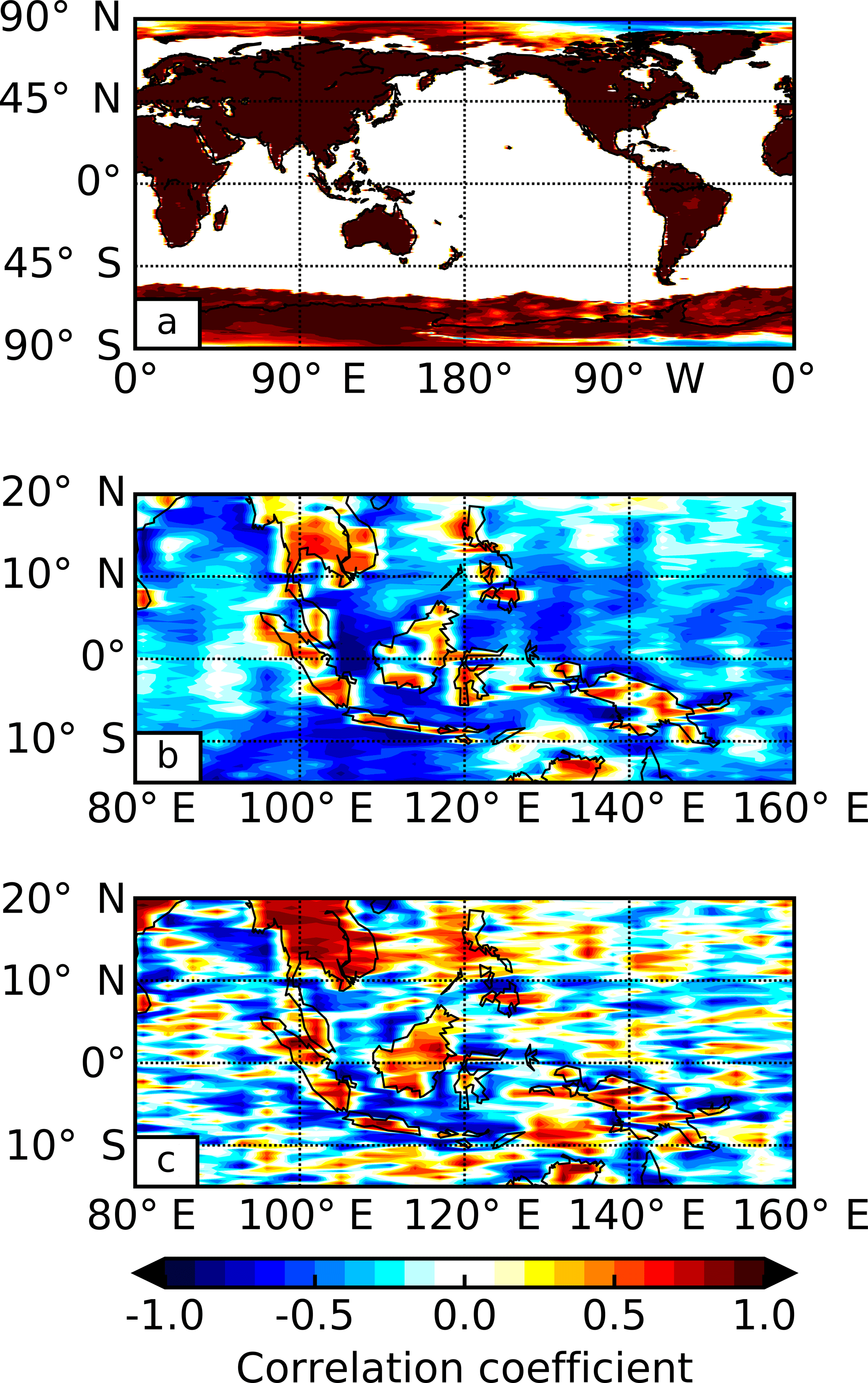
Figure 9Heterogeneous correlation maps for (a) the first principal component of outgoing long-wave radiation and global surface temperature, (b) the second principal component of outgoing long-wave radiation and cloud liquid water path in the Maritime Continent region (reversed in sign to aid comparisons) and (c) the second principal component of top-of-atmosphere albedo and cloud liquid water path in the Maritime Continent region.

Download

Table 1Maximum correlation coefficient and time lag at which it occurs from a cross-correlation between principal components (PCs) of modelled outgoing long-wave radiation (OLR) and PCs of modelled surface temperature, cloud liquid water path (LWP), cloud ice water path (IWP) and cloud top height (CTH).

Download Print Version | Download XLSX

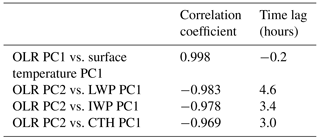
The cross-correlation of the second PC of OLR with the first PCs of modelled variables that are related to convective cloud development (LWP, IWP and CTH) reveals very high correlations but with substantial lag times (Table 1, rows 2–4). A lag between these variables is expected during convective cloud development, and the order in which the lags occur is consistent with the life cycle of a convective system. As locally driven convection initiates, water will begin to condense and cloud will develop at warm lower levels, causing the LWP to build first and the longest lag time. Once the convection breaks through the freezing level, further cloud development will mostly consist of ice crystals and the IWP will build, leading to a relatively shorter lag time. All the while, the vertical extent of the cloud is increasing and, as the convective system matures and produces an anvil, the CTH will reach a maximum, providing the shortest lag time. At this stage, as the convection dies and the CTH begins to reduce, one may expect the OLR to respond immediately but, curiously, a 3 h lag remains between the maximum correlation of OLR PC2 and CTH PC1.

A possible explanation for this remaining lag is provided by considering the changes in the environment of the upper troposphere after the convection dissipates. As the anvil cloud horizontally entrains into surrounding clear-sky regions it will evaporate, leading to an increase in upper tropospheric humidity (UTH). Using 1 year of long-wave water vapour (6.7 µm) and window (11 µm) channel radiances from multiple geostationary satellites spanning global longitude, Tian et al. (2004) showed that deep convection in the tropics acts to moisten the upper troposphere via the evaporation of anvil clouds generated by deep convection. This increase in UTH can be prevalent over large spatial extents and will delay the increase in OLR after the convective cloud has dissipated due to continued absorption of the more intense radiation originating from warmer, lower altitudes. The radiative heating that this provides leads to an increase in atmospheric stability and limits further cloud development, providing an important radiative–convective feedback mechanism for the diurnal cycle (Stephens et al., 2008). The study by Tian et al. (2004) suggested a lag of approximately 6 h between high cloud cover and UTH. In a similar but more spatially and temporally limited analysis, Soden (2000) suggested a lag time of approximately 2 h. In fact, the lag can be quite uncertain as it depends on the initial state of the atmosphere and spatial scale of convection (Ingram, 2015). The 3 h lag found here falls between these values and suggests that diurnal variations in OLR due to convective activity may remain tied to the UTH even when the convective cloud itself has dissipated.

To assess the spatial correlations we return to the Maritime Continent region where we know there are strong diurnal cycles in convective activity. The second PC of OLR correlated with the diurnal cycle of LWP at each grid point (Fig. 9b) shows the highest correlations in the same regions as the largest weights in the second OLR EOF. This indicates that this pattern of OLR variability is highly coupled to diurnal cloud development in these regions, as expected. Similar patterns are seen for IWP and CTH.

4.3.2 TOA albedo

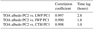
The cross-correlation of the second PC of TOA albedo with the first PCs of LWP, IWP and CTH reveals systematically higher correlations than the corresponding OLR correlations (Table 2). The order of the lag times amongst the cloud variables is maintained, but the lag times are shorter and only a 1 h lag remains between the TOA albedo and CTH. Unlike the OLR, the TOA albedo will not continue to respond in a similar way to the cloudy atmosphere once the cloud evaporates and the UTH increases. In fact, the opposite will occur as more solar radiation is absorbed in the humid environment. Remember that the second TOA albedo PC is also controlled by marine stratocumulus cloud that will not moisten the upper troposphere and may reduce the time lag between the variations in TOA albedo and CTH. The implication of this differing radiation response is that the diurnal changes in TOA albedo due to cloud development and dissipation are sharper and more immediate. Conversely, the OLR response is spread over a larger time and occurs later.

Table 2Same as Table 1, but for modelled top-of-atmosphere (TOA) albedo.

Download Print Version | Download XLSX

Similar to the second PC of OLR, the spatial correlation of the second PC of TOA albedo with the diurnal cycle of LWP at each grid point in the Maritime Continent region (Fig. 9c) shows the highest correlations in the same regions as the largest weights in the second TOA albedo EOF. Again, similar patterns are seen for the IWP and CTH in this region. In marine stratocumulus regions, however (not shown), the correlations are high for LWP but not for the other variables, demonstrating the value of assessing the extent of coupling with different data fields to identify unique physical processes. A schematic diagram summarizing the dominant processes controlling the OLR and TOA albedo, and their relation to other variables, is provided in Fig. 10.

Figure 10A schematic diagram showing the processes that control the first (a and b) and second (c and d) most dominant patterns in the diurnal variability of the outgoing long-wave radiation (OLR) (a and c) and top-of-atmosphere (TOA) albedo (b and d). Different arrow and Sun colours illustrate the change in solar zenith angle during the diurnal cycle and should not be interpreted as a change in wavelength. The separation of aerosol, surface and cloud reflection in the top right panel is for illustrative purposes only and does not relate to different parts of the diurnal cycle.

Download

4.3.3 Lag times in GERB and SEVIRI observations

We finally present the equivalent correlations and lag times in GERB observations of OLR and TOA albedo and SEVIRI observations of CTH for July 2006, with an emphasis on qualitative comparisons with the model results due to the different time periods and spatial regions considered. The intention is to identify whether the correlations and lag times are broadly consistent, to build confidence that the model is capable of capturing the physics of diurnal evolution.

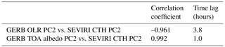
The observations (Table 3), just like the model (Tables 1 and 2), show that the magnitude of the maximum correlation coefficient with the CTH PC is larger for TOA albedo PC2 than OLR PC2. The lag time between the OLR PC2 and the CTH PC is 0.8 h longer in the observations than the model. For the TOA albedo, the lag time is the same. This supports the model finding that the TOA albedo responds more rapidly to cloud development than OLR and, if anything, suggests that the difference is even larger than the model indicates.

Table 3Same as Table 1, but for OLR and TOA albedo retrieved from Geostationary Earth Radiation Budget (GERB) observations, and CTH retrieved from Spinning Enhanced Visible and InfraRed Imager (SEVIRI) observations.

Download Print Version | Download XLSX