the Creative Commons Attribution 4.0 License.
the Creative Commons Attribution 4.0 License.
 | 14 Mar 2018
Emissions of trace gases from Australian temperate forest fires: emission factors and dependence on modified combustion efficiency
Elise-Andrée Guérette
Clare Paton-Walsh
Maximilien Desservettaz
Thomas E. L. Smith
Liubov Volkova
Christopher J. Weston
Carl P. Meyer
We characterised trace gas emissions from Australian temperate forest fires through a mixture of open-path Fourier transform infrared (OP-FTIR) measurements and selective ion flow tube mass spectrometry (SIFT-MS) and White cell FTIR analysis of grab samples. We report emission factors for a total of 25 trace gas species measured in smoke from nine prescribed fires. We find significant dependence on modified combustion efficiency (MCE) for some species, although regional differences indicate that the use of MCE as a proxy may be limited. We also find that the fire-integrated MCE values derived from our in situ on-the-ground open-path measurements are not significantly different from those reported for airborne measurements of smoke from fires in the same ecosystem. We then compare our average emission factors to those measured for temperate forest fires elsewhere (North America) and for fires in another dominant Australian ecosystem (savanna) and find significant differences in both cases. Indeed, we find that although the emission factors of some species agree within 20 %, including those of hydrogen cyanide, ethene, methanol, formaldehyde and 1,3-butadiene, others, such as acetic acid, ethanol, monoterpenes, ammonia, acetonitrile and pyrrole, differ by a factor of 2 or more. This indicates that the use of ecosystem-specific emission factors is warranted for applications involving emissions from Australian forest fires.
- Article
(3938 KB) -
Supplement
(388 KB) - BibTeX
- EndNote


Biomass burning emits a wide range of trace species, including greenhouse gases, particulate matter and volatile organic compounds (VOCs). Globally, fires are the second largest source of VOCs, with emissions estimated at 400 Tg yr−1 on average (Akagi et al., 2011; Yokelson et al., 2008). Fires are also the main driver of interannual variability for species such as carbon monoxide and particulate matter (Edwards et al., 2004, 2006; Voulgarakis et al., 2015).
Australia emits 7–8 % of global annual biomass burning carbon emissions (Ito and Penner, 2004; van der Werf et al., 2010). At a national level, average gross annual emissions of total carbon from fires (127 Tg C yr−1) actually exceed those from burning fossil fuels (95 Tg C yr−1) (Haverd et al., 2013). While net emissions of carbon from fires are lower due to regrowth (Haverd et al., 2013; Landry and Matthews, 2016), volatile organic species emitted by those fires are not subject to uptake by the regenerating vegetation and can therefore be considered net emissions.
The mix of VOCs emitted during biomass burning may be ecosystem-specific, with species such as monoterpenes being distilled from the vegetation as it is heated by the approaching fire (Ciccioli et al., 2014). Methanol, acetic acid, acetaldehyde, acetone and monoterpenes have all been detected from heated Eucalyptus leaves in laboratory experiments, with differences observed between fresh leaves and senescent leaves (Greenberg et al., 2006; Maleknia et al., 2007, 2009; Possell and Bell, 2013). Other factors that impact smoke composition include fuel composition (Coggon et al., 2016) and fire behaviour (Wooster et al., 2011). Changes in fire behaviour can be reflected in the combustion efficiency of the fire, i.e. in the proportion of total carbon that is emitted as CO2. A useful proxy for combustion efficiency is modified combustion efficiency (MCE), which is defined as the ratio of CO2 released to the sum of CO and CO2 (Hao and Ward, 1993; Yokelson et al., 1996). Emission factors of several trace gases have been found to correlate with MCE in a number of ecosystems (Akagi et al., 2013; Burling et al., 2011; Meyer et al., 2012).
The composition of fresh smoke matters as it affects plume chemistry as the smoke ages, contributing to varying rates of ozone and aerosol formation (Akagi et al., 2012; Alvarado et al., 2015; Yokelson et al., 2009) and elevated ozone and particulates downwind of the fires (Pfister et al., 2008; Yan et al., 2008).
Most of the area burnt in Australia annually is in the semi-arid and tropical savannas in the north of the country (Russell-Smith et al., 2007), but large bushfires also occur regularly in the temperate forests that cover extensive areas of the south-east of Australia (Cai et al., 2009). These fires can be intense enough to create pyroconvective lofting and inject smoke at high altitudes (Dirksen et al., 2009; Fromm et al., 2006; Guan et al., 2010; Siddaway and Petelina, 2011; de Laat et al., 2012) and are expected to become more frequent under a changing climate (Bradstock et al., 2009; Cai et al., 2009; Keywood et al., 2013; King et al., 2013). There has been growing interest in characterising the composition of smoke from Australian temperate forest fires in recent years, mostly arising from increased awareness of the significant impacts of bushfire smoke on regional air quality (Keywood et al., 2015; Price et al., 2012; Rea et al., 2016; Reisen et al., 2011, 2013) and its associated repercussions on human health (Johnston et al., 2012, 2014; Reid et al., 2016; Reisen and Brown, 2006; Reisen et al., 2015), coincident with a mandate for state agencies to increase prescribed burning in the wake of the catastrophic 2009 forest fires in Victoria (Teague et al., 2010). Prescribed burning is widely used in Australia as a means of reducing bushfire risk (Boer et al., 2009); however, these low-to-moderate-intensity fires often take place close to population centres, under weather conditions (low wind speeds, stable atmosphere) that are conducive to pollution build-up, sometimes on a regional scale (Williamson et al., 2016), with potential health impacts on nearby populations (Haikerwal et al., 2015).
Most of what is known about the VOC emissions from Australian temperate fires to date comes from opportunistic measurements of bushfire plumes impacting measurement sites such as the University of Wollongong (Paton-Walsh et al., 2005, 2008; Rea et al., 2016) or the Cape Grim Baseline Air Pollution Station (Lawson et al., 2015), or captured from space using satellite sensors (Glatthor et al., 2013; Young and Paton-Walsh, 2011). Dedicated field and laboratory measurement campaigns have mostly focused on greenhouse gases (Hurst et al., 1996; Possell et al., 2015; Surawski et al., 2015; Volkova et al., 2014).
Volkova et al. (2014) reported emission factors for carbon dioxide (CO2), carbon monoxide (CO), methane (CH4) and nitrous oxide (N2O) separately for burning fine fuels and logs from measurements made on the ground at prescribed fires in the state of Victoria. Surawski et al. (2015) measured emissions of CO2, CO, CH4 and N2O from fine Eucalyptus litter fuels in a combustion wind tunnel and found that emissions from these fuels vary depending on the mode of fire spread and on the phase of combustion. Possell et al. (2015) reported emission factors for CO2 and CO for several fuel classes combusted in a mass-loss calorimeter and estimated the total fraction of fuel carbon that would be emitted as CH4, particulates and non-methane hydrocarbons using a carbon mass balance approach. The only whole-fire emission factors available are those from Hurst et al. (1996), who sampled smoke plumes from fires in the greater Sydney region from an aircraft and reported emission factors for CO2, CO and CH4.
This paper presents results from a dedicated ground measurement programme that sampled smoke at several prescribed fires organised by the New South Wales (NSW) National Parks and Wildlife Service in the greater Sydney area and by the Department of Environment, Land, Water and Planning in the state of Victoria. Measurements made at a subset of these fires were presented in Paton-Walsh et al. (2014) along with a detailed description of the open-path Fourier transform infrared system (OP-FTIR) and a discussion of the uncertainties associated with deriving emission factors using this technique. Here, we present emission factors for 15 additional VOC species, measured by selected ion flow tube mass spectrometry (SIFT-MS) from grab samples collected at prescribed fires in NSW, as well as additional OP-FTIR results from fires in the state of Victoria. We then investigate the dependence of the measured emission factors on MCE, using all the data collected to date. We also compare the average MCE values observed in our ground measurements to MCE values reported for measurements from other platforms, including airborne measurements. Finally, we compare our average emission factors to values reported in the literature for other ecosystems. Currently, widely used compilations of emission factors (Akagi et al., 2011) do not include any results from Australian forests fires. In fact, the emission factors listed for temperate forests in Akagi et al. (2011) are sourced exclusively from measurements made at North American fires. We compare our results with the emission factors listed in Akagi et al. (2011) for temperate forests and to emission factors measured for Australian savanna fires (Smith et al., 2014) and find significant differences in both cases.
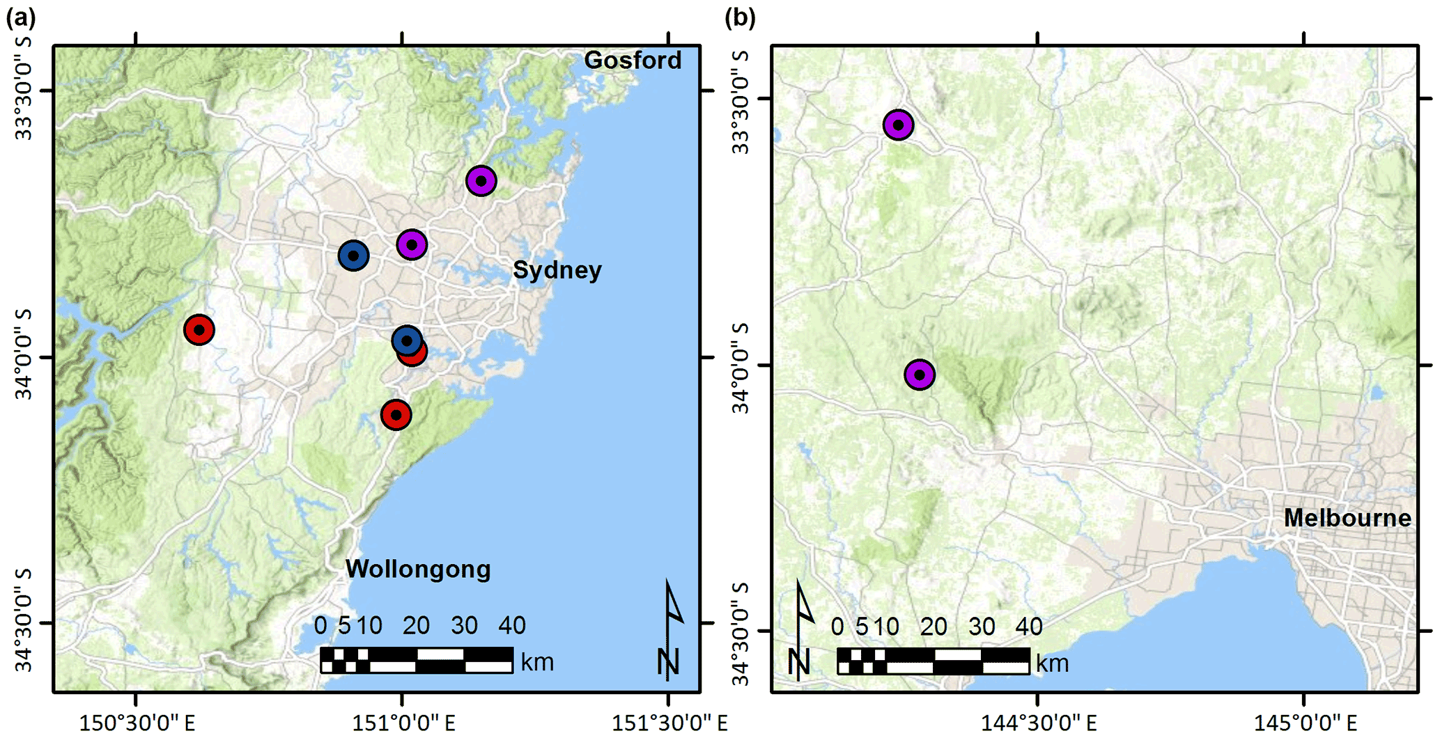
Figure 1Locations of the nine prescribed fires in Australian temperate forests sampled between 2010 and 2015. The NSW fires are in panel (a), and the fires in Victoria in panel (b). The red dots represent fires where both OP-FTIR and grab sampling took place, the blue dots indicate fires where only grab sampling took place, and the purple dots indicate fires where only OP-FTIR sampling took place.
2.1 Prescribed fires
Between 2010 and 2015, we sampled a total of nine prescribed fires in Australian temperate forests. Seven of those fires took place in NSW in 2010–2013; the other two fires were sampled in the state of Victoria in April 2015. The locations of the fires sampled are indicated on the maps shown in Fig. 1. All fires took place in variants of dry sclerophyll forests, dominated by eucalypt species. Table S1 in the Supplement lists the fires, their location, the dates on which they were sampled, the main vegetation type, the area burnt, the fuel loading, the time elapsed since the previous fire, the coordinates of the sampling sites and the method(s) of sampling deployed (these methods correspond to the colour coding on the maps in Fig. 1).
In NSW, all fires took place in the greater Sydney area, as seen in Fig. 1. Dominant overstorey species included eucalypts (including Eucalyptus, Corymbia and Angophora species), with Melaleuca, Acacia and Banksia species in the sub-canopy and the shrubby understorey. The ground cover was generally made up of native grasses and a litter of eucalypt leaves, bark and twigs, as well as fallen tree limbs of varying sizes.
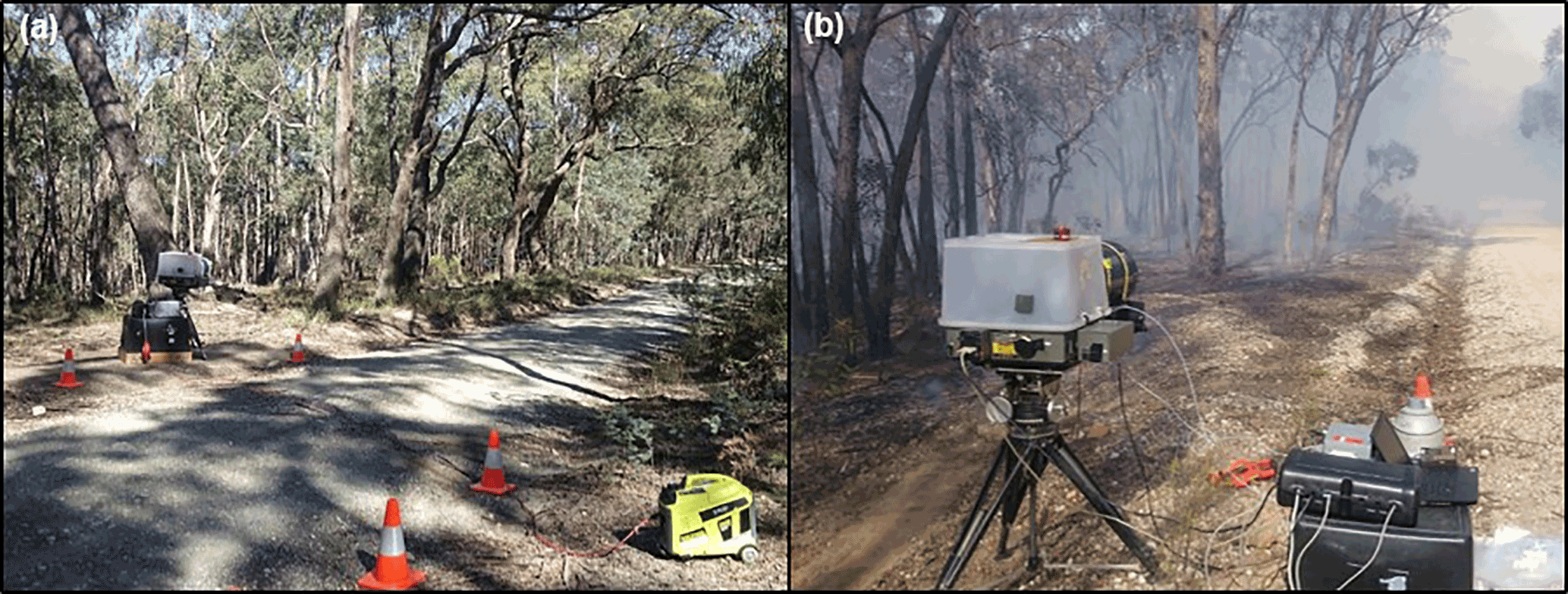
Figure 2The instrumental set-up for the open-path FTIR measurements of smoke in Greendale on 13 April 2015 (a) and Castlemaine on 23 April 2015 (b).
In Victoria, dominant overstorey species were E. radiata (Sieb. ex. DC.), E. obliqua (L'Hérit.), E. dives (Schau.), E. leucoxylon (F. Muell.) and E. macrorhyncha (F. Muell.). Acacia and Banksia species dominated the understorey. Ground cover was dominated by tree litter, with gorse (Ulex europaeus) and blackberry (Rubus fruticosus) recorded in some areas.
2.2 Open-path FTIR system (OP-FTIR)
An open-path FTIR system was deployed at five prescribed fires in NSW and at the two prescribed fires in Victoria, as indicated in the last column of Table S1 in the Supplement. The system used in this project is described in detail in Paton-Walsh et al. (2014). Briefly, the spectrometer (Bomem MB100-Series, 1 cm−1 resolution) has a built-in infrared source and is placed 20–50 m away from a set of retro-reflectors positioned so that smoke from the fire crosses the path in between. The system can run autonomously and records a spectrum consisting of three scans, approximately every 20 s. Ambient pressure and temperature are monitored at one end of the path, through a barometer (Vaisala PTB110) and a resistance temperature detector (RTD PT100) connected to the computer controlling the spectrometer via an I/O box. The output is logged at the same time resolution as the spectral measurements.
Typically, the system is set up and starts recording before the fire is ignited, and is left to run until mole fractions return to ambient values. As the measurement is integrated over a path of several metres and is continuous over the duration of the fire, the emissions measured using this technique are likely to capture smoke from all stages of the fire and therefore to be representative of the whole fire. One of the great advantages of OP-FTIR is that there is no sample capture, avoiding losses due to walls or sample lines.
In April 2015, the OP-FTIR was deployed at two prescribed burns in temperate forests in Victoria, several hundred kilometres away from the fires sampled in 2010–2013. The first fire, on 13 April, was near Greendale, Victoria, and the second, on 23 April, was in Kalimna Park, Castlemaine, Victoria (see Fig. 1 for a map of the locations). At the Greendale fire, the spectrometer was positioned along a fire trail and the retro-reflectors were installed 45 m away within the woodland area to be burned, so that both smoke and flames passed through the line of sight of the instrument. At the Castlemaine fire, both the spectrometer and the retro-reflectors were positioned along a fire trail downwind of the fire, so that smoke would blow through the 50 m measurement path. The instrument set-up at both fires is shown in Fig. 2. The details of the NSW deployments are in Paton-Walsh et al. (2014).
The OP-FTIR spectra collected during the fires were subsequently analysed to derive mole fractions of carbon dioxide (CO2), carbon monoxide (CO), methane (CH4), acetic acid (CH3COOH), ammonia (NH3), ethene (C2H4), formaldehyde (H2CO), formic acid (HCOOH) and methanol (CH3OH) using the Multiple Atmospheric Layer Transmission (MALT) model (Griffith, 1996; Griffith et al., 2012) and the spectral windows described in Paton-Walsh et al. (2014). The uncertainty on individual measurements is the error on the retrieval reported by MALT. For a complete uncertainty budget for the OP-FTIR measurements in smoke, see Appendix B of Paton-Walsh et al. (2014).
2.3 Grab sampling
A total of 67 smoke samples were collected over 7 days of sampling at five prescribed fires in NSW. Of those samples, over half were of well-mixed, rising smoke. The others were from various targets, including smouldering litter and logs and burning grass and shrubs. The number of samples collected at each fire is indicated in brackets in the last column of Table S1. Samples were collected in 600 mL glass flasks, except at the Gulguer plateau fire, where samples were collected in 1 L Tedlar bags. The glass flasks were pre-evacuated using a turbo-molecular pump (Pfeiffer TCS 010) prior to deployment to the fires and filled with smoke on site by opening them for a few seconds. No sample line was affixed to the flasks for sampling; flasks were positioned in the smoke prior to opening them. The bags were flushed with high-purity nitrogen and brought to the Gulguer fire where they were filled with smoke using a differential pressure system or “vacuum box” powered by a generator. As the generator had to be placed away from the fire, a sample line (∼ 5 m) was attached to the vacuum box. Filling the bags took a few minutes, and consequently, most samples were collected from large smouldering targets after the fire front had moved through the sampling area.
All grab samples were brought back to the lab and analysed within 24 h of collection. A FTIR spectrometer coupled to a White cell was used to measure carbon dioxide (CO2), carbon monoxide (CO), methane (CH4), ethane (C2H6) and ethene (C2H4). VOC mole fractions were measured using selective ion flow tube mass spectrometry (SIFT-MS).
2.3.1 FTIR spectrometer coupled to a White cell (White cell FTIR)
Mole fractions of CO2, CO, CH4, C2H6 and C2H4 in the grab samples of smoke collected at the fires were measured using a Bomem MB100-Series FTIR spectrometer (1 cm−1 resolution). This spectrometer is coupled to a multi-pass optical (White) cell with a path of 22.2 m and is fitted with an indium antimony (InSb) detector cooled with liquid nitrogen.
Part of the sample was transferred to the evacuated White cell and the temperature and pressure inside the cell were logged. Typical temperature and pressure inside the White cell were 22 ∘C and 220 hPa, respectively. A spectrum consisting of 78 scans was acquired for each grab sample. Mole fractions were retrieved using the MALT model (Griffith, 1996; Griffith et al., 2012). The uncertainty on individual grab sample measurements is taken as the error reported by MALT for the retrieval.
2.3.2 Selective ion flow tube mass spectrometry (SIFT-MS)
SIFT-MS is a technique for the online analysis of gas samples that is akin to the better-known proton-transfer-reaction mass spectrometry (PTR-MS) (Blake et al., 2009). Both instruments use chemical ionisation to ionise the VOCs present in air and both are equipped with quadrupole mass filters. The main advantage of SIFT-MS is its capability to switch between three reagent ions (H3O+, NO+ and ) within a single measurement cycle, allowing the detection of species such as acetylene and ethene in addition to the species commonly detected using PTR-MS within the same analysis. It does this by producing all three reagent ions simultaneously in a microwave discharge and then selecting one or the other (switching) using a quadrupole mass filter (the instrument therefore has two quadrupole mass filters). By contrast, PTR-MS is typically equipped with a hollow-cathode discharge that produces a pure stream of a single reagent ion (most commonly H3O+) and therefore requires a single quadrupole. Another difference is that PTR-MS uses a drift tube as its reaction chamber (in which ions are carried by an electric field), whereas SIFT-MS is equipped with a flow tube. The specific instrument used in this study (Syft Voice 100) uses a stream of helium and argon to thermalise and carry the ions (Milligan et al., 2007). This means that the instrument dilutes the sample by a factor that is a function of the pressure and temperature inside the flow tube, and of the flows of sample and carrier gases. This makes the instrument less sensitive than PTR-MS (Blake et al., 2009) but ideally suited for the analysis of highly polluted air, such as smoke samples. The flow tube dilution ratio under standard operating conditions is about 1 : 15.
The SIFT-MS was operated in multiple ion mode, targeting 18 VOC species. Table S2 lists the species targeted, the reagent ion used, the mass-to-charge ratios measured and the calibration factors used to quantify them. The list includes aromatic species, nitrogen-containing species, some oxygenated species, some small hydrocarbons and some biogenic species, targeting a breadth of chemical classes. The species targeted were for the most part the most abundant reported at their nominal molecular mass by Yokelson et al. (2013), who deployed extensive instrumentation in a laboratory setting and calculated emission factors for 357 species. A notable exception is the signal at NO+ 68, which is calibrated using isoprene, but is expected to be dominated by furan in smoke samples. Also, the signal at H3O+ 71 is expected to include 2-butenal as well as methacrolein (MACR) and methyl vinyl ketone (MVK). The measurement cycle took approximately 7 s to complete and was repeated eight times on each smoke sample. Mole fractions of VOCs were computed from raw SIFT-MS spectra using the calibration factors listed in Table S2. For each sample, an average mole fraction was calculated for each species by taking the mean over all repeats. The standard deviation of the mean was taken as the uncertainty on the average mole fraction. An average mole fraction was reported for a given species only if its signal-to-noise ratio was greater than 3, i.e. if the average signal was at least 3 times greater than the standard deviation of its mean.
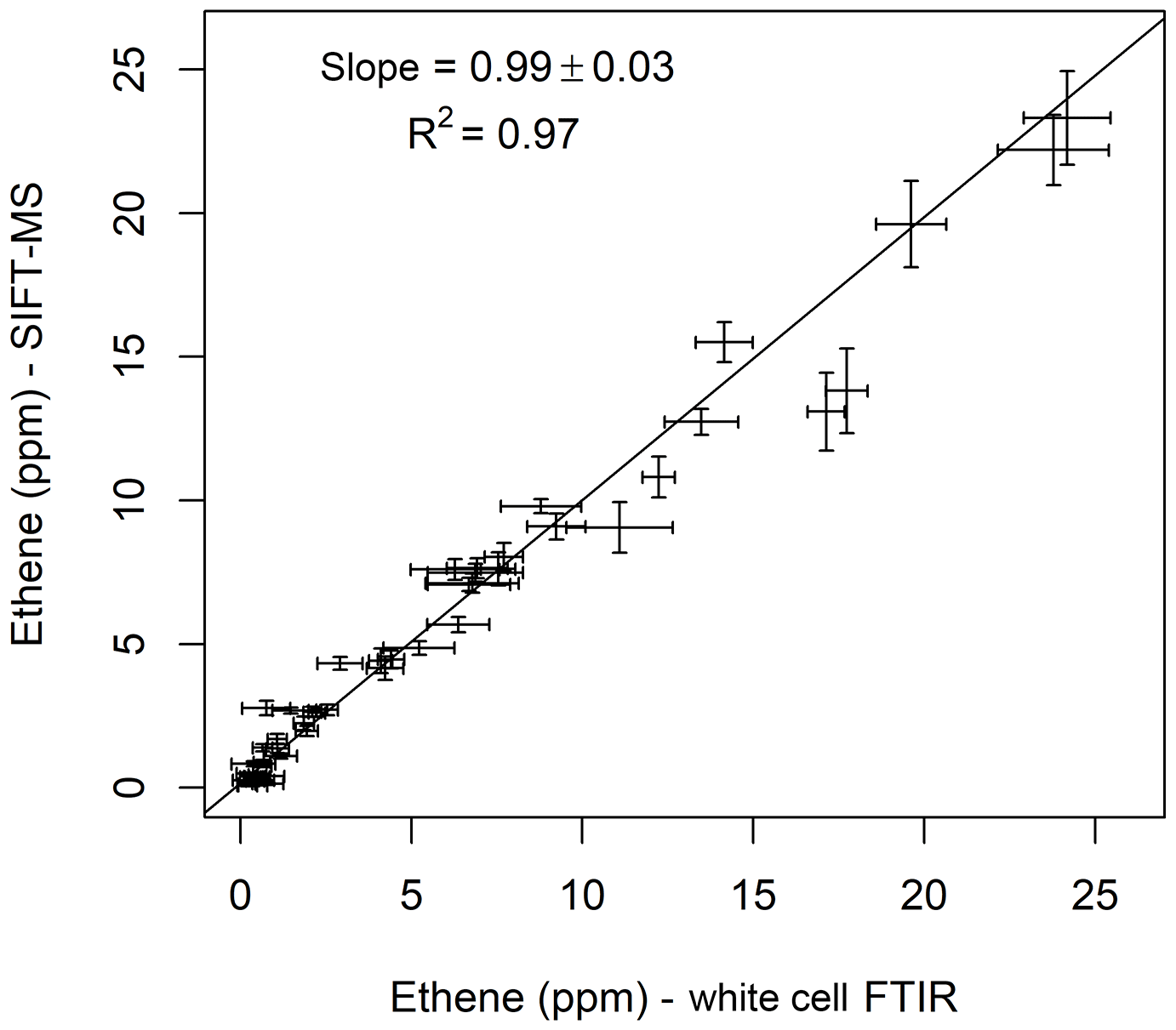
Figure 3Comparison of ethene mole fractions measured by SIFT-MS with those measured by White cell FTIR in grab samples of smoke collected at Australian temperate forest fires. Error bars for the SIFT-MS are the standard deviation of the measurement; for the White cell FTIR, they are the error on the retrieval. The line of best fit was determined using orthogonal regression.
The linearity of the SIFT-MS response was checked by plotting the mole fractions measured for ethene against those measured by White cell FTIR in the same grab samples. Figure 3 shows the good agreement for ethene between the two methods. The plot demonstrates that there was no loss of linearity in the SIFT-MS response even at high mole fractions, which is a result of the sample dilution that occurs within the flow tube of the instrument.
2.4 Determination of emission ratios (ERs)
Emission ratios (ERs) were derived by plotting VOC mole fractions against those of CO or CO2 (or another reference VOC species in some cases; see below) and applying an orthogonal regression. Orthogonal regression finds the best line of fit by minimising squared distances between (x,y) points and their projection on the line of best fit. The regression is also weighted by the uncertainties in both x and y, which, in this case, are the measurement uncertainties described above, so that the line of best fit has greater dependence on the more precise data points. The slope of the line of best fit is the emission ratio. As noted in a recent evaluation of linear regression techniques (Wu and Yu, 2018), the type of linear regression applied has little impact on the resulting slope as long as the correlation coefficient is high. For this reason, we chose pairs of species that were well correlated to derive emission ratios and do not report results when R2<0.5, as this should yield the most robust results. More generally, we chose to use linear regression to derive ERs instead of calculating a value from each measurement (Burling et al., 2011) because the background mole fractions of many measured species were poorly defined, often being below the detection limit of the SIFT-MS. Deriving emission ratio through regression without first subtracting background values introduces very little error (Wooster et al., 2011).
Emission ratios were derived from the open-path measurements for each fire separately. The mean ER from all the fires sampled is then our best estimate for the ecosystem. For the grab samples, emission ratios were derived for individual fires when possible; however, the VOC results from the targeted grab sampling were more highly variable than the open-path measurements in the well-mixed smoke, as is common for this type of sampling (Akagi et al., 2013; Burling et al., 2011; Yokelson et al., 2008, 2013). This resulted in poor correlations (R2<0.5) for some species for certain fires. Also, not every trace gas species was present at a detectable level in every sample. For some fires, this resulted in too few samples to allow an emission ratio to be meaningfully derived by regression for that species. As ERs were not successfully derived for each fire for some species, a mean ER was not necessarily the best estimate for the ecosystem. To derive a best estimate for the ecosystem, all valid samples were combined irrespective of which fire they were collected at and a single ER derived through orthogonal regression.
Certain VOC species measured in the grab samples did not correlate strongly with either CO or CO2. In those cases, emission ratios were derived using another reference species, e.g. an emission ratio to acetonitrile was derived for pyrrole, and ethene was used as a reference species to derive an emission ratio for benzene, 1,3-butadiene and acetylene. Good correlation between VOC species may indicate co-emission.
2.5 Determination of emission factors (EFs) and MCE
An emission factor (EF) is defined as the mass of trace gas of interest (X) released per amount of dry biomass burnt and is typically expressed in units of g kg−1:
This is a very direct method of estimating emissions, but can only be used if all the emissions are captured (so that the total mass of gas X can be measured) and if the mass of biomass burnt in the fire is known (Andreae and Merlet, 2001), which is rarely the case except in laboratory experiments. In the absence of such knowledge, the total mass of biomass burnt can be derived from the total mass of carbon emitted and the fractional carbon content of the biomass burnt (Fcarbon), which is sometimes measured but often estimated:
In this study, Fcarbon was assigned a value of 0.5, as in Akagi et al. (2011), Yokelson et al. (2011) and Paton-Walsh et al. (2014). Similarly, the total mass of carbon emitted by a fire is usually not known and is estimated by measuring the most abundant carbon-containing species emitted by the fire. The emission factor for species X is then
where MMX is the molar mass of the species of interest, 12 is the atomic mass of carbon and is the number of moles of species X emitted divided by the total number of moles of carbon emitted. In general, only a subset of the smoke from a fire is sampled. If that sample is representative of the whole fire, then the observed ratio of a species to the sum of all other species should be representative of the entire fire. can be calculated directly from the excess amounts measured:
where Δ[X] and Δ[Y] are the total excess mole fraction of the species of interest and of another carbon-containing species, respectively; NCy is the number of carbon atoms in species Y and the sum is over all carbon-containing species measured in the smoke. Equation (4) can also be written as
and it follows that the emission factor for a given species of interest can be calculated from the emission ratio of that species to the reference species and the emission factor of the reference species:
MCE is a proxy for combustion efficiency, which is defined as the proportion of total carbon emitted by a fire released as CO2. MCE is defined as the excess mole fraction of CO2 divided by the sum of the excess mole fractions of CO2 and CO (Hao and Ward, 1993; Yokelson et al., 1996):
When the fire is dominated by flaming combustion, the modified combustion efficiency is high, meaning that the emissions are dominated by CO2. The combustion efficiency decreases as smouldering combustion and emissions of CO become more dominant. Flaming combustion is generally associated with MCE values greater than 0.9 and smouldering combustion with values below 0.9 (Bertschi et al., 2003; Yokelson et al., 1996).
There are variants on how to apply the equations above; see Paton-Walsh et al. (2014) for a discussion. In this project, we chose the same approach as in Paton-Walsh et al. (2014) to process the open-path FTIR data and calculated emission factors for CO and CO2 using Eq. (4), with calculated using the total excess amounts of each gas detected by summing over the excess amounts from each measurement. The emission factors of other species were calculated using Eq. (6). Similarly, the MCE of a fire sampled by OP-FTIR was determined from the total excess amounts of CO2 and CO detected by the open-path system (i.e. by summing the excess amounts from each measurement recorded). These MCE values are used to determine whether the emission factors of the species measured by OP-FTIR have a dependence on MCE.
For grab samples, two variants of the analysis were completed. The first one was used to derive emission factors and MCE values to evaluate whether the emission factors of the species measured only in the grab samples have a dependence on MCE. For this analysis, emission factors for CO2, CO and CH4 were calculated for each individual grab sample using Eq. (4), with CT calculated as the sum of CO2, CO and CH4 only. Although many more carbon-containing species were measured in the grab samples, only CO2, CO and CH4 were successfully quantified in every single grab sample. For consistency, they were therefore the only species included in the calculation. Doing so inflates the emission factors by up to a few percent (<5 %) (Gilman et al., 2015; Yokelson et al., 2013). The emission factors for CO and CO2 were then used with Eq. (6) and the emission ratios determined for individual fires, to derive emission factors for each fire. MCE was calculated for each sample using Eq. (7) and an average value determined for each fire. These MCE values are indicative of the type of combustion (e.g. flaming vs. smouldering) captured by the grab sampling and are not necessarily representative of the whole fire. As an example, the average MCE of the grab samples collected at the Gulguer fire – where grab samples were mostly collected from smouldering logs – was 0.78 ± 0.09, whereas a fire-integrated value of 0.90 was measured by OP-FTIR (Paton-Walsh et al., 2014).
The second variant was used to determine ecosystem-average emission factors for the species measured only in the grab samples. In this case, we used Eq. (6) with the emission ratios derived from combining all data together, and the emission factors for CO and CO2 derived from the in situ OP-FTIR measurements at the NSW fires. If the emission ratio for a given VOC was derived using another VOC (instead of CO or CO2), their emission ratio was first converted to an emission ratio to CO or CO2 using the emission ratio of their reference VOC to CO or CO2. The uncertainty on the resulting emission ratio to CO (or CO2) was calculated by adding the uncertainties in quadrature.
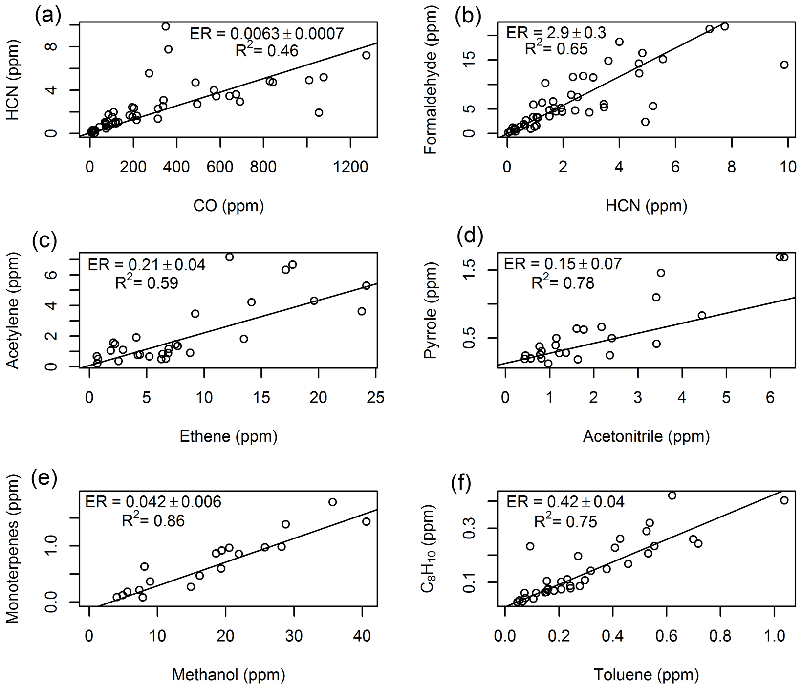
Figure 4Examples of “all data combined” correlations from the grab sample measurements. Panel (a) is hydrogen cyanide (HCN) to CO, (b) is formaldehyde to HCN, (c) is acetylene to ethene, (d) is pyrrole to acetonitrile, (e) is monoterpenes to methanol and (f) is the sum of C8H10 species to toluene.
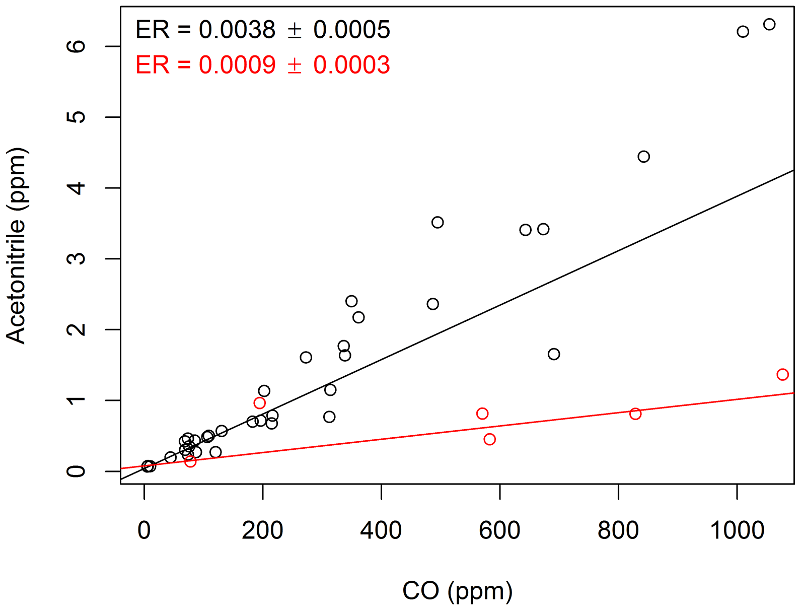
Figure 5ER for acetonitrile to CO for the Gulguer fire grab samples (in red) and for the other four fires (in black).
Table 1Summary of ERs determined for species measured by SIFT-MS and White cell FTIR in grab samples collected at the NSW fires. Mean ER is the average ER measured at individual fires. The “all data combined” ER was derived through orthogonal regression on all available samples irrespective of which fire they were collected at.
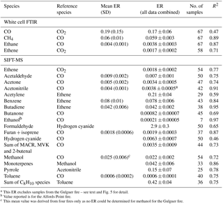
a This ER excludes samples from the Gulguer fire – see text and Fig. 5 for
detail.
b Value reported is for the Alfords Point fire.
c This mean value was derived from four fires only as no ER could be determined for methanol for the Gulguer
fire.
3.1 Emission ratios and emission factors determined from grab samples collected at prescribed fires in NSW and analysed using SIFT-MS and White cell FTIR
ERs were derived for all species measured in the grab samples by White cell FTIR and SIFT-MS as per Sect. 2.4. Emission ratios for individual fires, when available, are listed in Table S3. Table 1 lists the emission ratios derived from combining data from all fires (“all data combined”). When emission ratios for individual fires are available (see Table S3), the mean emission ratio is also included in Table 1. Figure S1 in the Supplement shows the correlation of ethane with CO for each of the five individual fires, and for all fires combined, as an example. Figure 4 shows the “all data combined” correlations for six species (hydrogen cyanide, formaldehyde, acetylene, pyrrole, monoterpenes and the sum of C8H10 species).
The emission ratios of some species show important site-to-site variability (see Table S3). For example, the emission ratio of CH4 to CO measured at Prospect Reservoir is lower than the average (0.06 (0.01); see Table S3). The site at Prospect Reservoir was mostly grassy, and the emission ratio measured there (0.037 ± 0.004) is close to the one measured in tussock- and hummock-grass savanna open woodland fires in northern Australia (0.040 ± 0.007) by Smith et al. (2014).
Similarly, the emission ratio of acetonitrile to CO is markedly lower at Gulguer fire than at the other fires. This could be due to the lower nitrogen content of logs compared to foliage and twigs (Snowdon et al., 2005; Susott et al., 1996), resulting in lower emissions of nitrogen-containing species (Coggon et al., 2016). The Gulguer fire samples are excluded from the emission ratio for acetonitrile derived from combining data from all fires, since including them results in R2<0.5. Figure 5 shows the correlations of acetonitrile with CO: the Gulguer fire is shown in red; the other four fires are shown in black. The emission ratio derived from the black line is not significantly different from the mean ER that includes the Gulguer fire data (see Table 1). Pyrrole showed the same behaviour against CO as acetonitrile. Its emission ratio was therefore derived to acetonitrile instead of CO.
Table 2Summary of open-path FTIR measurements at prescribed fires in temperate forests in the state of Victoria and comparison with similar results obtained at prescribed fires in New South Wales. Values in parentheses are standard deviations of the mean.
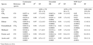
a Paton-Walsh et al. (2014).
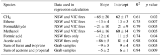
Table 3Summary of regression statistics for the emission factor dependence on MCE of carbon-containing species measured by open-path FTIR in temperate forest fires in Australia.
Despite this site-to-site variability in the emission ratio of certain species, the mean emission ratio is usually the same, within the uncertainties, as the value derived from combining samples from all fires. This indicates that the “all data combined” emission ratios listed in Table 1 are representative of the ecosystem sampled – a useful result since this is the only ER available for some species. Whole-fire emission factors were then calculated using the “all data combined” emission ratios listed in Table 1 and the average fire-integrated emission factors for CO and CO2 measured by OP-FTIR at the NSW fires by Paton-Walsh et al. (2014) and reproduced in the last column of Table 2. The resulting ecosystem-average emission factors for all VOC species are listed in Table 5.
3.2 Open-path FTIR results from prescribed fires in temperate forests in Victoria
All trace gases measured by OP-FTIR at the prescribed fires in Victoria exhibited strong correlations with either CO or CO2. Correlations between the measured species at the Castlemaine fire are shown in Fig. S2 as an example. The calculated emission ratios and emission factors are listed in Table 2.
There is little variability seen between the two fires sampled in Victoria. The emission ratios measured at the two fires are comparable, and the emission factors agree within their uncertainties. The emission ratios measured in Victoria are within the range of values measured at the NSW fires for all species except formic acid and acetic acid (Table 2). The average observed MCE of 0.92 at the Victorian fires is higher than that reported by Paton-Walsh et al. (2014) for the NSW fires (average 0.90, range of 0.88–0.91). The emission factors listed in Table 2 generally reflect this difference, with species typically associated with smouldering combustion having slightly lower emission factors at the Victorian fires. The differences are slight, however, and the emission factors from Victoria agree within the uncertainties with those from NSW. One major exception is acetic acid: its emission ratio at the fires in Victoria was double that seen at the NSW fires, and this is reflected in the emission factors. This indicates a difference in emissions from the different regions sampled that is not explained by the difference in modified combustion efficiency. The dependence of emission factors derived from the OP-FTIR measurements on MCE is explored more fully in the next section.
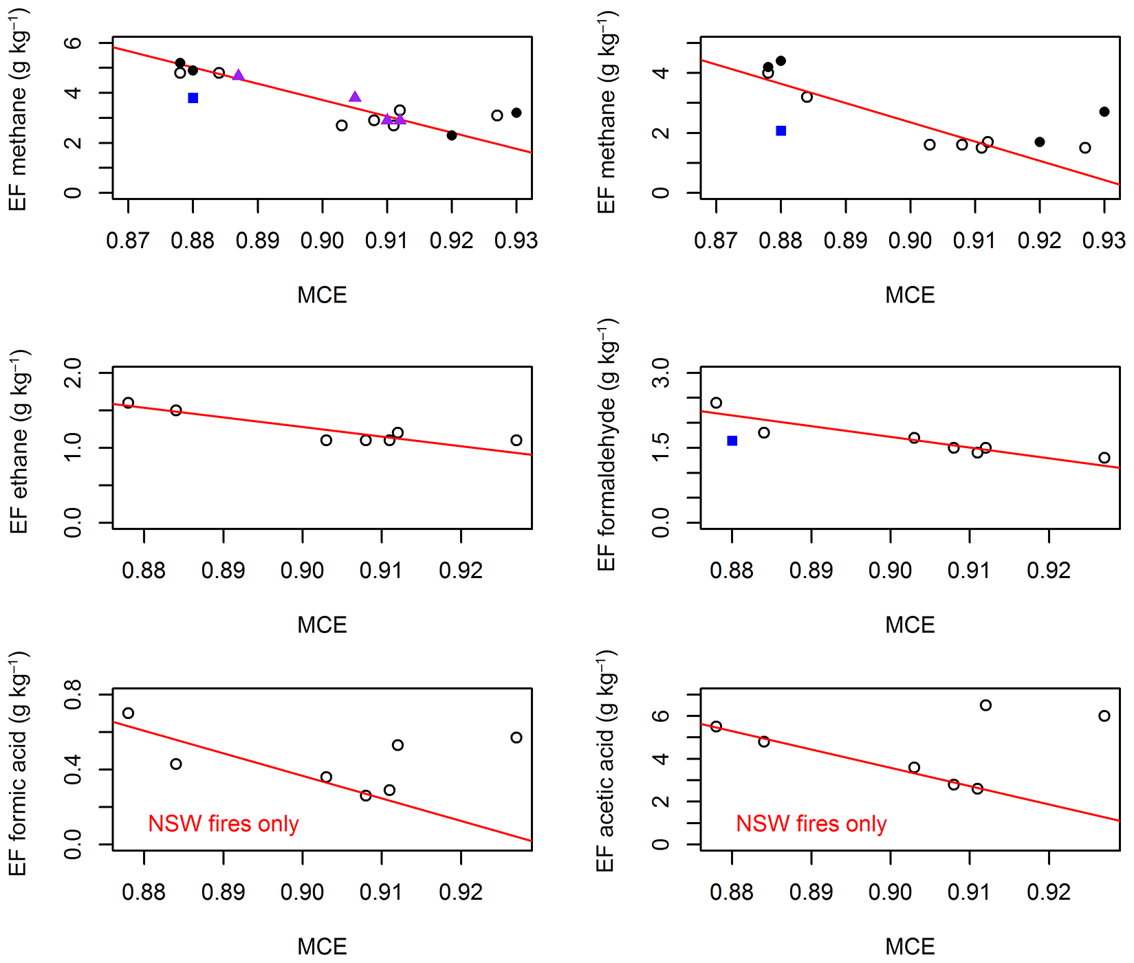
Figure 6Dependence of emission factors on MCE. Open circles represent the seven fires sampled using OP-FTIR with the line of best fit shown in red. For formic acid and acetic acid, this regression line was derived using the measurements from the NSW fires only. The black circles represent average results from grab samples at four fires (the grab sampling results from the Gulguer fire are either not available (methanol) or fall outside the range measured by OP-FTIR (methane) and therefore do not appear). The purple triangles represent the methane results from the airborne measurements of Hurst et al. (1996) and the blue squares represent the emission factors measured for methane, methanol and formaldehyde by Lawson et al. (2015) in a transported plume impacting the Cape Grim Baseline Air Pollution Station in Tasmania.
3.3 Dependence of emission factors of trace gases from Australian temperate forest fires on MCE
The MCE dependence of the emissions of carbon-containing species from all fires sampled using OP-FTIR as part of this ground-based study is explored in this section. The emission factors calculated for each fire sampled by OP-FTIR are plotted as a function of MCE in Fig. 6. The regression statistics are listed in Table 3. As the range of observed MCE is relatively narrow, the relationship is well represented using a linear regression. For larger MCE ranges, an exponential fit may be more appropriate (e.g. Meyer et al., 2012 suggest an exponential fit for CH4).
The magnitude of the slope and the intercept listed in Table 3 reflects the magnitude of the emission factor for that species. The strength of the relationship is judged from the coefficient of determination (R2) and the p value (the probability that there is no correlation between x and y). A poor R2 indicates that MCE alone cannot explain the variability in EFs.
For some species, there is no significant relationship with MCE when including data from all seven fires. This is the case for formic acid and acetic acid, for which significantly different emission ratios were measured at the fires in Victoria. Similarly, the emission factor for CH4 has a stronger relationship with MCE when considering only the NSW fires. This indicates that combustion efficiency is not the only factor that controls differences in emissions for these species.
For comparison purposes, the emission factors measured by Hurst et al. (1996) for CH4 and Lawson et al. (2015) for CH4, methanol and formaldehyde are also plotted in Fig. 6. Figure 6 also shows the average results derived for CH4 and methanol from the grab samples. The grab sampling results from the Gulguer fire are either not available (methanol) or fall outside the range measured by OP-FTIR (methane) and therefore do not appear in Fig. 6. The MCE-dependence of the species that were only measured in the grab samples (by SIFT-MS or White cell FTIR) was also tested. For this analysis, average values from the five fires were used, spanning a range of average MCE of 0.78 to 0.93. No statistically significant trend was found for acetaldehyde, acetonitrile, benzene, butadiene, ethane and toluene, but there were significant trends for the sum of furan and isoprene, and for the sum of acetone and propanal. The statistics for these trends are listed in Table 3. The MCE dependence of the other measured species could not be determined because fire-specific emission ratios were not available.
4.1 Comparison with MCE-dependent emission factors from North American temperate forests
The MCE dependence of emission factors listed in Table 3 was compared to those reported by Akagi et al. (2013) for fires in conifer forests in South Carolina and by Burling et al. (2011) for fires in conifer forests in North Carolina and for chaparral fires in California. There is considerable variability between the two North American studies, even for the similar conifer ecosystems sampled. Both studies found negative relationships to MCE for CH4 (with slopes ranging from −65 ± 13 to −96 ± 10), methanol (with slopes ranging from −21 ± 6 to −39 ± 2) and furan (−6 ± 3 to −8 ± 1). These results are consistent with the ones listed in Table 3 for these species, although the slope measured in Australian temperate forests for methanol is larger (−64 ± 16).
For other species, the results are mixed, with Akagi et al. (2013) finding no relationship to MCE for acetic acid but Burling et al. (2011) finding a strong one (with a slope of −45 ± 3 and R2 of 0.98) in a similar conifer ecosystem. This is analogous to the results presented here, where a strong relationship to MCE is found for a subset of the data (NSW fires only, slope of −86 ± 5, R2 of 0.98), but no relationship is found when all the fires are considered. For formic acid, both North American studies find a relationship for conifer forest fires (with slopes of −1.8 ± 0.6 and −3.1 ± 0.2), but Burling et al. (2011) found no relationship for chaparral fires. In this study, we find a relationship for the NSW fires but no relationship when including all fires.
Hurst et al. (1996)Lawson et al. (2015)Paton-Walsh et al. (2014)Rea et al. (2016)Akagi et al. (2011)Table 4Comparison of whole-fire MCE and whole-fire emission factors for CO2, CO and CH4 reported in the literature for fires in Australian temperate forests and temperate forests in North America.
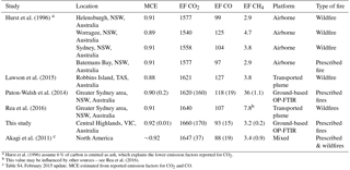
a Hurst et al. (1996) assume 6 % of carbon is emitted as ash, which explains the lower emission factors reported for
CO2.
b This value may be influenced by other sources – see
Rea et al. (2016).
c Table S4, February 2015 update. MCE estimated from reported emission factors for CO2 and CO.
For formaldehyde and ethene, Akagi et al. (2013) reports a weak or insignificant relationship to MCE, whereas Burling et al. (2011) reports strong relationships to MCE for both species for fires in a similar conifer ecosystem (with slopes of −21 ± 2 for formaldehyde and −11 ± 2 for ethene) and a weak or insignificant relationship to MCE for fires in chaparral. For fires in Australian temperate forests, we observed similar slopes of −21 ± 10 for formaldehyde and −13 ± 4 for ethene.
Akagi et al. (2013) report a slope of −16 ± 4 for acetone, which is larger than the one observed for the sum of acetone and propanal in this study (−5 ± 2). Akagi et al. (2013) also report significant relationships to MCE for ethane, benzene, toluene, xylenes, acetonitrile and acetaldehyde, whereas no relationship was observed for these species in our study.
Considering the variability of relationships to MCE observed even for similar ecosystems, it seems likely that other factors are influencing emissions. Burling et al. (2011) sampled spring fires, whereas Akagi et al. (2013) sampled autumn fires so it is possible that some of the variability is due to seasonal differences. In this study, fires were sampled over several years, both in spring (August–September) and in autumn (April–May). There is no obvious seasonal effect in the data; however, there seem to be regional effects, especially for formic acid and acetic acid, and these may be due to differences in vegetation. This variability limits the usefulness of MCE as a means of extrapolating emission factors for these species. Nevertheless, the MCE measured at a fire can be a good indication of whether a representative sample has been captured. This is explored in the next section by comparing MCE values observed from different measurement platforms for Australian temperate forest fires.
4.2 Comparison of MCE, CO2, CO and CH4 emission factors measured for Australian temperate ecosystems from various platforms
MCE and emission factors for CO2, CO and CH4 for Australian temperate ecosystems have been measured from a variety of platforms, including airborne measurements (Hurst et al., 1996) and measurements of plumes transported short distances to fixed monitoring stations (Lawson et al., 2015; Rea et al., 2016). Comparing these results to our ground-based measurements (see Table 4) reveals that there is a relatively small spread of MCE values measured for fires in Australian temperate ecosystems. There is no significant difference in the MCE observed for wild or prescribed fires, or between measurement platforms (Kruskal–Wallis rank sum test, p>0.7). This is in contrast with measurements conducted at prescribed fires in North America, where higher average MCE values were observed for airborne measurements than for open-path measurements on the ground (0.93 vs. 0.91 on average for the same fires in Akagi et al. (2014), for example). MCE values of 0.93 or greater for airborne measurements have also been reported by other US studies (Akagi et al., 2013; Burling et al., 2011). The top left panel of Fig. 6 shows the CH4 emission factors reported by Hurst et al. (1996) plotted alongside the OP-FTIR measurements conducted as part of this study and as part of Paton-Walsh et al. (2014). The agreement between the two platforms is excellent. The good agreement for MCE between platforms and fire type could be coincidental or an artefact of the sampling approaches, or may in fact indicate that the prescribed and wildfires sampled burnt at a similar MCE. Liu et al. (2017), studying wildfires in the western US, report EFs for PM1 that are a factor of 2 higher for wildfires than for prescribed fires burning at the same MCE but do not observe the same for trace gases such as CH4. No PM data are available from the studies listed in Table 4, but CH4 data are. The average emission factor measured for CH4 in Australian temperate forests is 3.5 (0.8) g kg−1 dry fuel burnt (this value excludes the emission factor reported by Rea et al. (2016) as it may have been influenced by other sources). The average for the ground-based OP-FTIR measurements is 3.5 (0.9) g kg−1 dry fuel burnt. These are in excellent agreement with the emission factor for CH4 of 3.4 (0.9) g kg−1 dry fuel burnt listed for temperate forests in Akagi et al. (2011).
4.3 Comparison of VOC emission ratios and emission factors measured for temperate ecosystems
Measurements of VOC emission factors have been more limited for Australian temperate forests. Enhancement ratios to CO for methanol, ammonia, formic acid, formaldehyde, acetylene, ethene and ethane were measured in lofted plumes from wildfires by ground-based solar remote sensing Fourier transform spectrometry (Paton-Walsh et al., 2005, 2008) and satellite-based spectroscopic measurements (Glatthor et al., 2013; Young and Paton-Walsh, 2011). These were compared to the emission ratios measured in fresh smoke by OP-FTIR in NSW by Paton-Walsh et al. (2014). They found good agreement for methanol and formaldehyde, and evidence for depletion of ammonia and ethene and formation of formic acid in aged smoke.
Table 5Comparison of VOC emission ratios and emission factors reported in the literature for fires in temperate forests in Australia and in North America. ERs are in mol mol−1 and EFs are in g kg−1 dry fuel burnt. Unidentified species that are likely to contribute to the signal measured by SIFT-MS are listed by their molar mass in the last column.
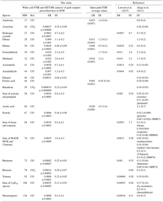
The only other study to have reported emission factors for a significant number of trace gas species is that of Lawson et al. (2015). They report emission ratios and emission factors for trace gases and aerosol from opportunistic measurement of a biomass burning plume impacting Cape Grim Baseline Air Pollution Station in Tasmania in February 2006. The plume was advected to the station from a fire in coastal heath on a nearby island, mostly at night (from 23:00 until 09:00 AEST). The vegetation burnt in the Robbins Island fire is similar to what typically burns in a prescribed fire, so their emission ratios and emission factors for VOCs are listed alongside ours in Table 5. Emission factors from Akagi et al. (2011) are also included for comparison. For some of the species measured by SIFT-MS in this study and by PTR-MS in Lawson et al. (2015), the reported emission factors are sum measurements of several species, including potential contributions from unidentified compounds. In these cases, the emission factors of all species that could contribute were sourced from Akagi et al. (2011) and listed in the last column of Table 5.
There is considerable variability in the emission factors listed in Table 5, and most species agree within their stated uncertainties. Nevertheless, comparing average values highlights potential differences between emissions from Australian temperate forests and emissions from North American temperate forests. Emission factors for both hydrogen cyanide and ethene are in excellent agreement, and emission factors for methanol, formaldehyde and 1,3-butadiene are within 20 % of each other. Emission factors for ethane, acetylene and toluene also agree quite well, being within about 30 % of each other. However, Australian forest fires potentially emit 50 % more formic acid, twice as much acetic acid and ammonia, less than half as much ethanol and monoterpenes, and 2–10 times more acetonitrile and pyrrole than North American fires.
Nitrogen-containing VOCs make little contribution to the overall reactivity of a smoke plume (Gilman et al., 2015). Acetonitrile has an atmospheric lifetime on the order of months and is a tracer for long-range transport of biomass plumes (Bange and Williams, 2000), whereas more reactive nitrogen-containing species may be tracers for fresh plumes (Coggon et al., 2016; Gilman et al., 2015). Higher emissions may affect estimates of plume age based on these species. The difference with the North American fires may be due to higher fuel nitrogen content. Acacias are nitrogen-fixing species that have high leaf N content (1.50–3.55 %) which is partly conserved through leaf fall, leading to higher nitrogen in the leaf litter (Snowdon et al., 2005). Acacias are some of the dominant understorey species in the forests investigated in this study, and their presence may have contributed to the high emissions of nitrogen-containing species; however, without fuel composition measurements, it is impossible to draw definitive conclusions.
The initial mixture of trace gases emitted by a fire is one of the factors (along with meteorology and the presence of other sources) that influences plume aging (Akagi et al., 2012; Jaffe and Wigder, 2012) and air quality outcomes downwind of the fires. The use of Australian-specific emission factors is therefore recommended in studies looking at the regional impact of fires in Australian temperate forests.
4.4 Comparison with emission factors reported for Australian savanna
As mentioned earlier, most of the area burnt in Australia annually is in the semi-arid and tropical savannas in the north of the country. A number of studies have characterised smoke from these fires (Desservettaz et al., 2017; Hurst et al., 1994a, b, 1996; Meyer et al., 2012; Paton-Walsh et al., 2010; Shirai et al., 2003; Smith et al., 2014; Wang et al., 2017a, b). Smith et al. (2014) used an OP-FTIR system to derive emission factors for CO2, CO, CH4, ethane, ethene, acetylene, formaldehyde, methanol, formic acid, acetic acid, ammonia and hydrogen cyanide. Comparing our OP-FTIR emission factors for temperate forests listed in Table 5 to those reported in Table 5 of Smith et al. (2014) indicates that both ecosystems have similar emission factors for formaldehyde and hydrogen cyanide (1.7 (0.4) vs. 1.6 (0.4) and 0.7 (0.2) vs. 0.5 (0.3) g kg−1 dry fuel burnt). Methane, methanol and ammonia show high variability in both ecosystems, and although the emission factors measured for temperate forests fires are higher, the emission factors agree within the uncertainties quoted (3.5 (0.9) vs. 2.2 (1.2), 2 (1) vs. 1.1 (0.8) and 1.6 (0.6) vs. 0.7 (0.4) g kg−1 dry fuel burnt for methane, methanol and ammonia, respectively). The comparison also reveals that fires in Australian temperate forests emit up to 5 times more ethane, 3 times more acetic acid, formic acid and acetylene, and twice as much ethene as Australian savanna fires on a kilogram of dry fuel basis. This highlights the need for ecosystem-specific emission factors for Australia, especially when looking at regional impacts of biomass burning events.
In this study, emission factors were derived for a total of 25 trace gas species using a mixture of in situ open-path FTIR and grab sampling at nine prescribed fires in Australian temperate forests. MCE values measured during these ground-based measurements were not significantly different from those reported in the literature from airborne measurements, which contrasts with what has been observed in temperate ecosystems in North America. The emission factors for CH4, ethene, formaldehyde, methanol, formic acid, acetic acid, the sum of furan and isoprene and the sum of acetone and propanal exhibited significant MCE dependence, although there were regional differences for formic acid, acetic acid and CH4 that indicate that the use of MCE may be of limited use to extrapolate emission factors. There were also differences between the MCE dependences observed in this study compared to those observed for fires in North American temperate ecosystems.
The average emission factors measured for Australian temperate forest fires were compared to those measured for fires in North American temperate ecosystems. The average emission factors for hydrogen cyanide and ethene were in excellent agreement, and those of methanol, formaldehyde, ethane, toluene and 1,3-butadiene were in good agreement (within 30 %). The emission factors measured in this study for other species, however, indicate that Australian temperate forests may emit 50 % more formic acid, twice as much acetic acid and ammonia, half as much ethanol and monoterpenes, and 2–10 times more acetonitrile and pyrrole than North American fires on a per kilogram of dry fuel burnt basis.
We also find that the emission factors for hydrogen cyanide and formaldehyde for Australian temperate forest fires are in excellent agreement with those measured for Australian savanna fires, but that the forest fires have emission factors that are up to 5 times higher for ethane, 3 times higher for acetic acid, formic acid and acetylene, and 2 times higher for ethene.
These differences would impact plume chemistry and influence air quality outcomes downwind of the fires. We therefore recommend that the emission factors presented here and in other studies such as those of Lawson et al. (2015) and Paton-Walsh et al. (2014) be used in studies of biomass burning that require ecosystem-specific emission factors to represent emissions from Australian forest fires.
All the emission ratios and the emission factors measured as part of this study are summarised in *.csv files provided as a Supplement to the main text.
The supplement related to this article is available online at: https://doi.org/10.5194/acp-18-3717-2018-supplement.
EAG contributed to field work in NSW, oversaw collection, instrumental analysis and data analysis for the grab samples, contributed to QA/QC of all data and wrote the paper. CPW conceived of the project, contributed to field work, oversaw measurements, spectral analysis, data analysis and QA/QC for all open-path FTIR measurements. MJD deployed the open-path system at fires in Victoria and contributed to data analysis. TELS contributed to FTIR spectral analysis and MCE analysis. LV, CJW and CPM coordinated with the Department of Environment, Land, Water and Planning to make attendance at the fires in Victoria possible and contributed details of vegetation at the fires in Victoria. All authors contributed to paper editing.
The authors declare that they have no conflict of interest.
For the NSW fires, the authors would like to acknowledge Sharon Evans,
Bill Sullivan and Simon Hawkes from the New South Wales National Parks and
Wildlife Service for allowing us to make measurements at their prescribed
burns and providing copies of their burn plans. Thanks are also due to
Melanie Cameron, Dagmar Kubistin, Paul Taglieri and Rachel Stevens from the
University of Wollongong and Grant Edwards and Cheryl Tang from Macquarie
University for help with grab sample collection. For the fires in Victoria,
we thank Elizabeth Ashman from the Department of Environment, Land, Water and
Planning as well as Doreena Dominick and Kaitlyn Lieschke from the University
of Wollongong. We would also like to acknowledge Travis Naylor and David Griffith
for helpful MALT discussions and Graham Kettlewell and Martin Riggenbach
for technical support. This work was funded by the Australian
Research Council as a small component of the Discovery Project DP110101948
(NSW fires) and as part of the Smoke Emission and Transport Modelling project
commissioned and funded by the Department of Environment, Land, Water and
Planning, Victoria. We also acknowledge the Clean Air and Urban Landscapes
Hub of Australia's National Environmental Science Program for funding the
further analysis of the results that was required to produce this paper.
Edited by: Alexander Laskin
Reviewed by: Nic Surawski, Vanessa Selimovic and two anonymous referees
Akagi, S. K., Yokelson, R. J., Wiedinmyer, C., Alvarado, M. J., Reid, J. S., Karl, T., Crounse, J. D., and Wennberg, P. O.: Emission factors for open and domestic biomass burning for use in atmospheric models, Atmos. Chem. Phys., 11, 4039–4072, https://doi.org/10.5194/acp-11-4039-2011, 2011. a, b, c, d, e, f, g, h, i
Akagi, S. K., Craven, J. S., Taylor, J. W., McMeeking, G. R., Yokelson, R. J., Burling, I. R., Urbanski, S. P., Wold, C. E., Seinfeld, J. H., Coe, H., Alvarado, M. J., and Weise, D. R.: Evolution of trace gases and particles emitted by a chaparral fire in California, Atmos. Chem. Phys., 12, 1397–1421, https://doi.org/10.5194/acp-12-1397-2012, 2012. a, b
Akagi, S. K., Yokelson, R. J., Burling, I. R., Meinardi, S., Simpson, I., Blake, D. R., McMeeking, G. R., Sullivan, A., Lee, T., Kreidenweis, S., Urbanski, S., Reardon, J., Griffith, D. W. T., Johnson, T. J., and Weise, D. R.: Measurements of reactive trace gases and variable O3 formation rates in some South Carolina biomass burning plumes, Atmos. Chem. Phys., 13, 1141–1165, https://doi.org/10.5194/acp-13-1141-2013, 2013. a, b, c, d, e, f, g, h, i
Akagi, S. K., Burling, I. R., Mendoza, A., Johnson, T. J., Cameron, M., Griffith, D. W. T., Paton-Walsh, C., Weise, D. R., Reardon, J., and Yokelson, R. J.: Field measurements of trace gases emitted by prescribed fires in southeastern US pine forests using an open-path FTIR system, Atmos. Chem. Phys., 14, 199–215, https://doi.org/10.5194/acp-14-199-2014, 2014. a
Alvarado, M. J., Lonsdale, C. R., Yokelson, R. J., Akagi, S. K., Coe, H., Craven, J. S., Fischer, E. V., McMeeking, G. R., Seinfeld, J. H., Soni, T., Taylor, J. W., Weise, D. R., and Wold, C. E.: Investigating the links between ozone and organic aerosol chemistry in a biomass burning plume from a prescribed fire in California chaparral, Atmos. Chem. Phys., 15, 6667–6688, https://doi.org/10.5194/acp-15-6667-2015, 2015. a
Andreae, M. O. and Merlet, P.: Emission of trace gases and aerosols from biomass burning, Global Biogeochem. Cy., 15, 955–966, https://doi.org/10.1029/2000gb001382, 2001. a
Bange, H. and Williams, J.: New Directions: Acetonitrile in atmospheric and biogeochemical cycles, Atmos. Environ., 34, 4959–4960, https://doi.org/10.1016/S1352-2310(00)00364-2, 2000. a
Bertschi, I., Yokelson, R. J., Ward, D. E., Babbitt, R. E., Susott, R. A., Goode, J. G., and Hao, W. M.: Trace gas and particle emissions from fires in large diameter and belowground biomass fuels, J. Geophys. Res.-Atmos., 108, 8472, https://doi.org/10.1029/2002jd002100, 2003. a
Blake, R. S., Monks, P. S., and Ellis, A. M.: Proton-Transfer Reaction Mass Spectrometry, Chem. Rev., 109, 861–896, https://doi.org/10.1021/cr800364q, 2009. a, b
Boer, M. M., Sadler, R. J., Wittkuhn, R. S., McCaw, L., and Grierson, P. F.: Long-term impacts of prescribed burning on regional extent and incidence of wildfires-Evidence from 50 years of active fire management in SW Australian forests, Forest Ecol. Manag., 259, 132–142, https://doi.org/10.1016/j.foreco.2009.10.005, 2009. a
Bradstock, R. A., Cohn, J. S., Gill, A. M., Bedward, M., and Lucas, C.: Prediction of the probability of large fires in the Sydney region of south-eastern Australia using fire weather, Int. J. Wildland Fire, 18, 932–943, https://doi.org/10.1071/WF08133, 2009. a
Burling, I. R., Yokelson, R. J., Akagi, S. K., Urbanski, S. P., Wold, C. E., Griffith, D. W. T., Johnson, T. J., Reardon, J., and Weise, D. R.: Airborne and ground-based measurements of the trace gases and particles emitted by prescribed fires in the United States, Atmos. Chem. Phys., 11, 12197–12216, https://doi.org/10.5194/acp-11-12197-2011, 2011. a, b, c, d, e, f, g, h, i
Cai, W., Cowan, T., and Raupach, M.: Positive Indian Ocean Dipole events precondition southeast Australia bushfires, Geophys. Res. Lett., 36, L19710, https://doi.org/10.1029/2009GL039902, 2009. a, b
Ciccioli, P., Centritto, M., and Loreto, F.: Biogenic volatile organic compound emissions from vegetation fires, Plant Cell Environ., 37, 1810–1825, https://doi.org/10.1111/pce.12336, 2014. a
Coggon, M. M., Veres, P. R., Yuan, B., Koss, A., Warneke, C., Gilman, J. B., Lerner, B. M., Peischl, J., Aikin, K. C., Stockwell, C. E., Hatch, L. E., Ryerson, T. B., Roberts, J. M., Yokelson, R. J., and de Gouw, J. A.: Emissions of nitrogen-containing organic compounds from the burning of herbaceous and arboraceous biomass: Fuel composition dependence and the variability of commonly used nitrile tracers, Geophys. Res. Lett., 43, 9903–9912, https://doi.org/10.1002/2016GL070562, 2016. a, b, c
de Laat, A. T. J., Stein Zweers, D. C., Boers, R., and Tuinder, O. N. E.: A solar escalator: Observational evidence of the self-lifting of smoke and aerosols by absorption of solar radiation in the February 2009 Australian Black Saturday plume, J. Geophys. Res.-Atmos., 117, D04204, https://doi.org/10.1029/2011JD017016, 2012. a
Desservettaz, M., Paton-Walsh, C., Griffith, D. W. T., Kettlewell, G., Keywood, M. D., Vanderschoot, M. V., Ward, J., Mallet, M. D., Milic, A., Miljevic, B., Ristovski, Z. D., Howard, D., Edwards, G. C., and Atkinson, B.: Emission factors of trace gases and particles from tropical savanna fires in Australia, J. Geophys. Res.-Atmos., 122, 6059–6074, https://doi.org/10.1002/2016JD025925, 2017. a
Dirksen, R. J., Folkert Boersma, K., de Laat, J., Stammes, P., van der Werf, G. R., Val Martin, M., and Kelder, H. M.: An aerosol boomerang: Rapid around-the-world transport of smoke from the December 2006 Australian forest fires observed from space, J. Geophys. Res.-Atmos., 114, D21201, https://doi.org/10.1029/2009JD012360, 2009. a
Edwards, D. P., Emmons, L. K., Hauglustaine, D. A., Chu, D. A., Gille, J. C., Kaufman, Y. J., Pétron, G., Yurganov, L. N., Giglio, L., Deeter, M. N., Yudin, V., Ziskin, D. C., Warner, J., Lamarque, J. F., Francis, G. L., Ho, S. P., Mao, D., Chen, J., Grechko, E. I., and Drummond, J. R.: Observations of carbon monoxide and aerosols from the Terra satellite: Northern Hemisphere variability, J. Geophys. Res.-Atmos., 109, D24202, https://doi.org/10.1029/2004JD004727, 2004. a
Edwards, D. P., Pétron, G., Novelli, P. C., Emmons, L. K., Gille, J. C., and Drummond, J. R.: Southern Hemisphere carbon monoxide interannual variability observed by Terra/Measurement of Pollution in the Troposphere (MOPITT), J. Geophys. Res.-Atmos., 111, D16303, https://doi.org/10.1029/2006JD007079, 2006. a
Fromm, M., Tupper, A., Rosenfeld, D., Servranckx, R., and McRae, R.: Violent pyro-convective storm devastates Australia's capital and pollutes the stratosphere, Geophys. Res. Lett., 33, L05815, https://doi.org/10.1029/2005GL025161, 2006. a
Gilman, J. B., Lerner, B. M., Kuster, W. C., Goldan, P. D., Warneke, C., Veres, P. R., Roberts, J. M., de Gouw, J. A., Burling, I. R., and Yokelson, R. J.: Biomass burning emissions and potential air quality impacts of volatile organic compounds and other trace gases from fuels common in the US, Atmos. Chem. Phys., 15, 13915–13938, https://doi.org/10.5194/acp-15-13915-2015, 2015. a, b, c
Glatthor, N., Höpfner, M., Semeniuk, K., Lupu, A., Palmer, P. I., McConnell, J. C., Kaminski, J. W., von Clarmann, T., Stiller, G. P., Funke, B., Kellmann, S., Linden, A., and Wiegele, A.: The Australian bushfires of February 2009: MIPAS observations and GEM-AQ model results, Atmos. Chem. Phys., 13, 1637–1658, https://doi.org/10.5194/acp-13-1637-2013, 2013. a, b
Greenberg, J. P., Friedli, H., Guenther, A. B., Hanson, D., Harley, P., and Karl, T.: Volatile organic emissions from the distillation and pyrolysis of vegetation, Atmos. Chem. Phys., 6, 81–91, https://doi.org/10.5194/acp-6-81-2006, 2006. a
Griffith, D. W. T.: Synthetic Calibration and Quantitative Analysis of Gas-Phase FT-IR Spectra, Appl. Spectrosc., 50, 59–70, 1996. a, b
Griffith, D. W. T., Deutscher, N. M., Caldow, C., Kettlewell, G., Riggenbach, M., and Hammer, S.: A Fourier transform infrared trace gas and isotope analyser for atmospheric applications, Atmos. Meas. Tech., 5, 2481–2498, https://doi.org/10.5194/amt-5-2481-2012, 2012. a, b
Guan, H., Esswein, R., Lopez, J., Bergstrom, R., Warnock, A., Follette-Cook, M., Fromm, M., and Iraci, L. T.: A multi-decadal history of biomass burning plume heights identified using aerosol index measurements, Atmos. Chem. Phys., 10, 6461–6469, https://doi.org/10.5194/acp-10-6461-2010, 2010. a
Haikerwal, A., Reisen, F., Sim, M. R., Abramson, M. J., Meyer, C. P., Johnston, F. H., and Dennekamp, M.: Impact of smoke from prescribed burning: Is it a public health concern?, JAPCA J. Air Waste Ma., 65, 592–598, https://doi.org/10.1080/10962247.2015.1032445, 2015. a
Hao, W. M. and Ward, D. E.: Methane production from global biomass burning, J. Geophys. Res.-Atmos., 98, 20657–20661, https://doi.org/10.1029/93jd01908, 1993. a, b
Haverd, V., Raupach, M. R., Briggs, P. R., J. G. Canadell., Davis, S. J., Law, R. M., Meyer, C. P., Peters, G. P., Pickett-Heaps, C., and Sherman, B.: The Australian terrestrial carbon budget, Biogeosciences, 10, 851–869, https://doi.org/10.5194/bg-10-851-2013, 2013. a, b
Hurst, D., Griffith, D. T., Carras, J., Williams, D., and Fraser, P.: Measurements of trace gases emitted by Australian savanna fires during the 1990 dry season, J. Atmos. Chem., 18, 33–56, https://doi.org/10.1007/bf00694373, 1994a. a
Hurst, D. F., Griffith, D. W. T., and Cook, G. D.: Trace gas emissions from biomass burning in tropical Australian savannas, J. Geophys. Res.-Atmos., 99, 16441–16456, https://doi.org/10.1029/94jd00670, 1994b. a
Hurst, D. F., Griffith, D. W. T., and Cook, G. D.: Trace-Gas Emissions from Biomass Burning in Australia, in: Biomass Burning and Global Change, edited by: Levine, J. S., The MIT Press, London, UK, 1996. a, b, c, d, e, f, g, h
Ito, A. and Penner, J. E.: Global estimates of biomass burning emissions based on satellite imagery for the year 2000, J. Geophys. Res.-Atmos., 109, D14S05, https://doi.org/10.1029/2003jd004423, 2004. a
Jaffe, D. A. and Wigder, N. L.: Ozone production from wildfires: A critical review, Atmos. Environ., 51, 1–10, https://doi.org/10.1016/j.atmosenv.2011.11.063, 2012. a
Johnston, F. H., Henderson, S. B., Chen, Y., Randerson, J. T., Marlier, M., DeFries, R. S., Kinney, P., Bowman, D. M., and Brauer, M.: Estimated Global Mortality Attributable to Smoke from Landscape Fires, Environ.Health Persp., 120, 695–701, https://doi.org/10.1289/ehp.1104422, 2012. a
Johnston, F. H., Purdie, S., Jalaludin, B., Martin, K. L., Henderson, S. B., and Morgan, G. G.: Air pollution events from forest fires and emergency department attendances in Sydney, Australia 1996–2007: a case-crossover analysis, Environ. Health, 13, 105, https://doi.org/10.1186/1476-069x-13-105, 2014. a
Keywood, M., Kanakidou, M., Stohl, A., Dentener, F., Grassi, G., Meyer, C. P., Torseth, K., Edwards, D., Thompson, A. M., Lohmann, U., and Burrows, J.: Fire in the Air-Biomass burning impacts in a changing climate, Crit. Rev. Env. Sci. Tec., 43, 40–83, https://doi.org/10.1080/10643389.2011.604248, 2013. a
Keywood, M., Cope, M., Meyer, C. P. M., Iinuma, Y., and Emmerson, K.: When smoke comes to town: The impact of biomass burning smoke on air quality, Atmos. Environ., 121, 13–21, https://doi.org/10.1016/j.atmosenv.2015.03.050, 2015. a
King, K. J., Cary, G. J., Bradstock, R. A., and Marsden-Smedley, J. B.: Contrasting fire responses to climate and management: insights from two Australian ecosystems, Glob. Change Biol., 19, 1223–1235, https://doi.org/10.1111/gcb.12115, 2013. a
Landry, J.-S. and Matthews, H. D.: Non-deforestation fire vs. fossil fuel combustion: the source of CO2 emissions affects the global carbon cycle and climate responses, Biogeosciences, 13, 2137–2149, https://doi.org/10.5194/bg-13-2137-2016, 2016. a
Lawson, S. J., Keywood, M. D., Galbally, I. E., Gras, J. L., Cainey, J. M., Cope, M. E., Krummel, P. B., Fraser, P. J., Steele, L. P., Bentley, S. T., Meyer, C. P., Ristovski, Z., and Goldstein, A. H.: Biomass burning emissions of trace gases and particles in marine air at Cape Grim, Tasmania, Atmos. Chem. Phys., 15, 13393–13411, https://doi.org/10.5194/acp-15-13393-2015, 2015. a, b, c, d, e, f
Liu, X., Huey, L. G., Yokelson, R. J., Selimovic, V., Simpson, I. J., Müller, M., Jimenez, J. L., Campuzano-Jost, P., Beyersdorf, A. J., Blake, D. R., Butterfield, Z., Choi, Y., Crounse, J. D., Day, D. A., Diskin, G. S., Dubey, M. K., Fortner, E., Hanisco, T. F., Hu, W., King, L. E., Kleinman, L., Meinardi, S., Mikoviny, T., Onasch, T. B., Palm, B. B., Peischl, J., Pollack, I. B., Ryerson, T. B., Sachse, G. W., Sedlacek, A. J., Shilling, J. E., Springston, S., St. Clair, J. M., Tanner, D. J., Teng, A. P., Wennberg, P. O., Wisthaler, A., and Wolfe, G. M.: Airborne measurements of western U.S. wildfire emissions: Comparison with prescribed burning and air quality implications, J. Geophys. Res.-Atmos., 122, 6108–6129, https://doi.org/10.1002/2016JD026315, 2017. a
Maleknia, S. D., Bell, T. L., and Adams, M. A.: PTR-MS analysis of reference and plant-emitted volatile organic compounds, Int. J. Mass Spectrometry, 262, 203–210, https://doi.org/10.1016/j.ijms.2006.11.010, 2007. a
Maleknia, S. D., Bell, T. L., and Adams, M. A.: Eucalypt smoke and wildfires: Temperature dependent emissions of biogenic volatile organic compounds, Int. J. Mass Spectrometry, 279, 126–133, https://doi.org/10.1016/j.ijms.2008.10.027, 2009. a
Meyer, C. P., Cook, G. D., Reisen, F., Smith, T. E. L., Tattaris, M., Russell-Smith, J., Maier, S. W., Yates, C. P., and Wooster, M. J.: Direct measurements of the seasonality of emission factors from savanna fires in northern Australia, J. Geophys. Res.-Atmos., 117, D20305, https://doi.org/10.1029/2012jd017671, 2012. a, b, c
Milligan, D. B., Francis, G. J., Prince, B. J., and McEwan, M. J.: Demonstration of Selected Ion Flow Tube MS Detection in the Parts per Trillion Range, Anal. Chem., 79, 2537–2540, https://doi.org/10.1021/ac0622678, 2007. a
Paton-Walsh, C., Jones, N. B., Wilson, S. R., Haverd, V., Meier, A., Griffith, D. W. T., and Rinsland, C. P.: Measurements of trace gas emissions from Australian forest fires and correlations with coincident measurements of aerosol optical depth, J. Geophys. Res., 110, D24305, https://doi.org/10.1029/2005jd006202, 2005. a, b
Paton-Walsh, C., Wilson, S. R., Jones, N. B., and Griffith, D. W. T.: Measurement of methanol emissions from Australian wildfires by ground-based solar Fourier transform spectroscopy, Geophys. Res. Lett., 35, L08810, https://doi.org/10.1029/2007gl032951, 2008. a, b
Paton-Walsh, C., Deutscher, N. M., Griffith, D. W. T., Forgan, B. W., Wilson, S. R., Jones, N. B., and Edwards, D. P.: Trace gas emissions from savanna fires in northern Australia, J. Geophys. Res.-Atmos., 115, D16314, https://doi.org/10.1029/2009JD013309, 2010. a
Paton-Walsh, C., Smith, T. E. L., Young, E. L., Griffith, D. W. T., and Guérette, É.-A.: New emission factors for Australian vegetation fires measured using open-path Fourier transform infrared spectroscopy – Part 1: Methods and Australian temperate forest fires, Atmos. Chem. Phys., 14, 11313–11333, https://doi.org/10.5194/acp-14-11313-2014, 2014. a, b, c, d, e, f, g, h, i, j, k, l, m, n, o
Pfister, G. G., Wiedinmyer, C., and Emmons, L. K.: Impacts of the fall 2007 California wildfires on surface ozone: Integrating local observations with global model simulations, Geophys. Res. Lett., 35, L19814, https://doi.org/10.1029/2008gl034747, 2008. a
Possell, M. and Bell, T. L.: The influence of fuel moisture content on the combustion of Eucalyptus foliage, Int. J. Wildland Fire, 22, 343–352, https://doi.org/10.1071/WF12077, 2013. a
Possell, M., Jenkins, M., Bell, T. L., and Adams, M. A.: Emissions from prescribed fires in temperate forest in south-east Australia: implications for carbon accounting, Biogeosciences, 12, 257–268, https://doi.org/10.5194/bg-12-257-2015, 2015. a, b
Price, O. F., Williamson, G. J., Henderson, S. B., Johnston, F., and Bowman, D. M. J. S.: The Relationship between Particulate Pollution Levels in Australian Cities, Meteorology, and Landscape Fire Activity Detected from MODIS Hotspots, PLOS ONE, 7, e47327, https://doi.org/10.1371/journal.pone.0047327, 2012. a
Rea, G., Paton-Walsh, C., Turquety, S., Cope, M., and Griffith, D.: Impact of the New South Wales fires during October 2013 on regional air quality in eastern Australia, Atmos. Environ., 131, 150–163, https://doi.org/10.1016/j.atmosenv.2016.01.034, 2016. a, b, c, d, e, f
Reid, C. E., Brauer, M., Johnston, F. H., Jerrett, M., Balmes, J. R., and Elliott, C.: Critical review of health impacts of wildfire smoke exposure, Environ. Health Persp., 124, 1334–1343, https://doi.org/10.1289/ehp.1409277, 2016. a
Reisen, F. and Brown, S. K.: Implications for Community Health from Exposure to Bushfire Air Toxics, Environ. Chem., 3, 235–243, https://doi.org/10.1071/EN06008, 2006. a
Reisen, F., Meyer, C. P., McCaw, L., Powell, J. C., Tolhurst, K., Keywood, M. D., and Gras, J. L.: Impact of smoke from biomass burning on air quality in rural communities in southern Australia, Atmos. Environ., 45, 3944–3953, https://doi.org/10.1016/j.atmosenv.2011.04.060, 2011. a
Reisen, F., Meyer, C. P., and Keywood, M. D.: Impact of biomass burning sources on seasonal aerosol air quality, Atmos. Environ., 67, 437–447, https://doi.org/10.1016/j.atmosenv.2012.11.004, 2013. a
Reisen, F., Duran, S. M., Flannigan, M., Elliott, C., and Rideout, K.: Wildfire smoke and public health risk, Int. J. Wildland Fire, 24, 1029–1044, https://doi.org/10.1071/WF15034, 2015. a
Russell-Smith, J., Yates, C. P., Whitehead, P. J., Smith, R., Craig, R., Allan, G. E., Thackway, R., Frakes, I., Cridland, S., Meyer, M. C. P., and Gill, A. M.: Bushfires 'down under': patterns and implications of contemporary Australian landscape burning, Int. J. Wildland Fire, 16, 361–377, https://doi.org/10.1071/WF07018, 2007. a
Shirai, T., Blake, D. R., Meinardi, S., Rowland, F. S., Russell-Smith, J., Edwards, A., Kondo, Y., Koike, M., Kita, K., Machida, T., Takegawa, N., Nishi, N., Kawakami, S., and Ogawa, T.: Emission estimates of selected volatile organic compounds from tropical savanna burning in northern Australia, J. Geophys. Res.-Atmos., 108, 8406, https://doi.org/10.1029/2001JD000841, 2003. a
Siddaway, J. M. and Petelina, S. V.: Transport and evolution of the 2009 Australian Black Saturday bushfire smoke in the lower stratosphere observed by OSIRIS on Odin, J. Geophys. Res., 116, D06203, https://doi.org/10.1029/2010JD015162, 2011. a
Smith, T. E. L., Paton-Walsh, C., Meyer, C. P., Cook, G. D., Maier, S. W., Russell-Smith, J., Wooster, M. J., and Yates, C. P.: New emission factors for Australian vegetation fires measured using open-path Fourier transform infrared spectroscopy – Part 2: Australian tropical savanna fires, Atmos. Chem. Phys., 14, 11335–11352, https://doi.org/10.5194/acp-14-11335-2014, 2014. a, b, c, d, e
Snowdon, P., Ryan, P., and Raison, J.: Review of the C:N Ratios in Vegetation, Litter and Soil Under Australian Native Forests and Plantations, Tech. Rep. National Carbon Accounting System Technical Report No. 45, Department of the Environment and Heritage, available at: http://www.fullcam.com/FullCAMServer/Help/reps/TR45 (last access: 8 March 2018), 2005. a, b
Surawski, N. C., Sullivan, A. L., Meyer, C. P., Roxburgh, S. H., and Polglase, P. J.: Greenhouse gas emissions from laboratory-scale fires in wildland fuels depend on fire spread mode and phase of combustion, Atmos. Chem. Phys., 15, 5259–5273, https://doi.org/10.5194/acp-15-5259-2015, 2015. a, b
Susott, R. A., Olbu, G. J., Baker, S. P., Ward, D. E., Kauffman, J. B., and Shea, R. W.: Carbon, hydrogen, nitrogen, and thermogravimetric analysis of tropical ecosystem biomass, in: Biomass Burning and Global Change, edited by: Levine, J. S., vol. 1, chap. 24, 249–259, The MIT Press, Cambridge, Mass., 1996. a
Teague, B., McLeod, R., Pascoe, S., and of Victoria, P.: Final Report, available at: http://royalcommission.vic.gov.au/Commission-Reports/Final-Report.html (last access: 8 March 2018), 2010. a
van der Werf, G. R., Randerson, J. T., Giglio, L., Collatz, G. J., Mu, M., Kasibhatla, P. S., Morton, D. C., DeFries, R. S., Jin, Y., and van Leeuwen, T. T.: Global fire emissions and the contribution of deforestation, savanna, forest, agricultural, and peat fires (1997–2009), Atmos. Chem. Phys., 10, 11707–11735, https://doi.org/10.5194/acp-10-11707-2010, 2010. a
Volkova, L., Meyer, C. P., Murphy, S., Fairman, T., Reisen, F., and Weston, C.: Fuel reduction burning mitigates wildfire effects on forest carbon and greenhouse gas emission, Int. J. Wildland Fire, 23, 771–780, https://doi.org/10.1071/WF14009, 2014. a, b
Voulgarakis, A., Marlier, M. E., Faluvegi, G., Shindell, D. T., Tsigaridis, K., and Mangeon, S.: Interannual variability of tropospheric trace gases and aerosols: The role of biomass burning emissions, J. Geophys. Res.-Atmos., 120, 7157–7173, https://doi.org/10.1002/2014JD022926, 2015. a
Wang, X., Meyer, C. P., Reisen, F., Keywood, M., Thai, P. K., Hawker, D. W., Powell, J., and Mueller, J. F.: Emission Factors for Selected Semivolatile Organic Chemicals from Burning of Tropical Biomass Fuels and Estimation of Annual Australian Emissions, Environ. Sci. Technol., 51, 9644–9652, https://doi.org/10.1021/acs.est.7b01392, 2017a. a
Wang, X., Thai, P. K., Mallet, M., Desservettaz, M., Hawker, D. W., Keywood, M., Miljevic, B., Paton-Walsh, C., Gallen, M., and Mueller, J. F.: Emissions of Selected Semivolatile Organic Chemicals from Forest and Savannah Fires, Environ. Sci. Technol., 51, 1293–1302, https://doi.org/10.1021/acs.est.6b03503, 2017b. a
Williamson, G. J., Bowman, D. M. J. S., Price, O. F., Henderson, S. B., and Johnston, F. H.: A transdisciplinary approach to understanding the health effects of wildfire and prescribed fire smoke regimes, Environ. Res. Lett., 11, 125009, https://doi.org/10.1088/1748-9326/11/12/125009, 2016. a
Wooster, M. J., Freeborn, P. H., Archibald, S., Oppenheimer, C., Roberts, G. J., Smith, T. E. L., Govender, N., Burton, M., and Palumbo, I.: Field determination of biomass burning emission ratios and factors via open-path FTIR spectroscopy and fire radiative power assessment: headfire, backfire and residual smouldering combustion in African savannahs, Atmos. Chem. Phys., 11, 11591–11615, https://doi.org/10.5194/acp-11-11591-2011, 2011. a, b
Wu, C. and Yu, J. Z.: Evaluation of linear regression techniques for atmospheric applications: the importance of appropriate weighting, Atmos. Meas. Tech., 11, 1233–1250,https://doi.org/10.5194/amt-11-1233-2018, 2018. a
Yan, B., Zheng, M., Hu, Y. T., Lee, S., Kim, H. K., and Russell, A. G.: Organic composition of carbonaceous aerosols in an aged prescribed fire plume, Atmos. Chem. Phys., 8, 6381–6394, https://doi.org/10.5194/acp-8-6381-2008, 2008. a
Yokelson, R. J., Griffith, D. W. T., and Ward, D. E.: Open-path Fourier transform infrared studies of large-scale laboratory biomass fires, J. Geophys. Res., 101, 21067–21080, https://doi.org/10.1029/96jd01800, 1996. a, b, c
Yokelson, R. J., Christian, T. J., Karl, T. G., and Guenther, A.: The tropical forest and fire emissions experiment: laboratory fire measurements and synthesis of campaign data, Atmos. Chem. Phys., 8, 3509–3527, https://doi.org/10.5194/acp-8-3509-2008, 2008. a, b
Yokelson, R. J., Crounse, J. D., DeCarlo, P. F., Karl, T., Urbanski, S., Atlas, E., Campos, T., Shinozuka, Y., Kapustin, V., Clarke, A. D., Weinheimer, A., Knapp, D. J., Montzka, D. D., Holloway, J., Weibring, P., Flocke, F., Zheng, W., Toohey, D., Wennberg, P. O., Wiedinmyer, C., Mauldin, L., Fried, A., Richter, D., Walega, J., Jimenez, J. L., Adachi, K., Buseck, P. R., Hall, S. R., and Shetter, R.: Emissions from biomass burning in the Yucatan, Atmos. Chem. Phys., 9, 5785–5812, https://doi.org/10.5194/acp-9-5785-2009, 2009. a
Yokelson, R. J., Burling, I. R., Urbanski, S. P., Atlas, E. L., Adachi, K., Buseck, P. R., Wiedinmyer, C., Akagi, S. K., Toohey, D. W., and Wold, C. E.: Trace gas and particle emissions from open biomass burning in Mexico, Atmos. Chem. Phys., 11, 6787–6808, https://doi.org/10.5194/acp-11-6787-2011, 2011. a
Yokelson, R. J., Burling, I. R., Gilman, J. B., Warneke, C., Stockwell, C. E., de Gouw, J., Akagi, S. K., Urbanski, S. P., Veres, P., Roberts, J. M., Kuster, W. C., Reardon, J., Griffith, D. W. T., Johnson, T. J., Hosseini, S., Miller, J. W., Cocker III, D. R., Jung, H., and Weise, D. R.: Coupling field and laboratory measurements to estimate the emission factors of identified and unidentified trace gases for prescribed fires, Atmos. Chem. Phys., 13, 89–116, https://doi.org/10.5194/acp-13-89-2013, 2013. a, b, c
Young, E. and Paton-Walsh, C.: Emission Ratios of the Tropospheric Ozone Precursors Nitrogen Dioxide and Formaldehyde from Australia's Black Saturday Fires, Atmosphere, 2, 617–632, 2011. a, b