the Creative Commons Attribution 3.0 License.
the Creative Commons Attribution 3.0 License.
Diurnal, synoptic and seasonal variability of atmospheric CO2 in the Paris megacity area
Irène Xueref-Remy
Elsa Dieudonné
Cyrille Vuillemin
Morgan Lopez
Christine Lac
Martina Schmidt
Marc Delmotte
Frédéric Chevallier
François Ravetta
Olivier Perrussel
Philippe Ciais
François-Marie Bréon
Grégoire Broquet
Michel Ramonet
T. Gerard Spain
Christophe Ampe
Most of the global fossil fuel CO2 emissions arise from urbanized and industrialized areas. Bottom-up inventories quantify them but with large uncertainties. In 2010–2011, the first atmospheric in situ CO2 measurement network for Paris, the capital of France, began operating with the aim of monitoring the regional atmospheric impact of the emissions coming from this megacity. Five stations sampled air along a northeast–southwest axis that corresponds to the direction of the dominant winds. Two stations are classified as rural (Traînou – TRN; Montgé-en-Goële – MON), two are peri-urban (Gonesse – GON; Gif-sur-Yvette – GIF) and one is urban (EIF, located on top of the Eiffel Tower). In this study, we analyze the diurnal, synoptic and seasonal variability of the in situ CO2 measurements over nearly 1 year (8 August 2010–13 July 2011). We compare these datasets with remote CO2 measurements made at Mace Head (MHD) on the Atlantic coast of Ireland and support our analysis with atmospheric boundary layer height (ABLH) observations made in the center of Paris and with both modeled and observed meteorological fields. The average hourly CO2 diurnal cycles observed at the regional stations are mostly driven by the CO2 biospheric cycle, the ABLH cycle and the proximity to urban CO2 emissions. Differences of several µmol mol−1 (ppm) can be observed from one regional site to the other. The more the site is surrounded by urban sources (mostly residential and commercial heating, and traffic), the more the CO2 concentration is elevated, as is the associated variability which reflects the variability of the urban sources. Furthermore, two sites with inlets high above ground level (EIF and TRN) show a phase shift of the CO2 diurnal cycle of a few hours compared to lower sites due to a strong coupling with the boundary layer diurnal cycle. As a consequence, the existence of a CO2 vertical gradient above Paris can be inferred, whose amplitude depends on the time of the day and on the season, ranging from a few tenths of ppm during daytime to several ppm during nighttime. The CO2 seasonal cycle inferred from monthly means at our regional sites is driven by the biospheric and anthropogenic CO2 flux seasonal cycles, the ABLH seasonal cycle and also synoptic variations. Enhancements of several ppm are observed at peri-urban stations compared to rural ones, mostly from the influence of urban emissions that are in the footprint of the peri-urban station. The seasonal cycle observed at the urban station (EIF) is specific and very sensitive to the ABLH cycle. At both the diurnal and the seasonal scales, noticeable differences of several ppm are observed between the measurements made at regional rural stations and the remote measurements made at MHD, that are shown not to define background concentrations appropriately for quantifying the regional (∼ 100 km) atmospheric impact of urban CO2 emissions. For wind speeds less than 3 m s−1, the accumulation of local CO2 emissions in the urban atmosphere forms a dome of several tens of ppm at the peri-urban stations, mostly under the influence of relatively local emissions including those from the Charles de Gaulle (CDG) Airport facility and from aircraft in flight. When wind speed increases, ventilation transforms the CO2 dome into a plume. Higher CO2 background concentrations of several ppm are advected from the remote Benelux–Ruhr and London regions, impacting concentrations at the five stations of the network even at wind speeds higher than 9 m s−1. For wind speeds ranging between 3 and 8 m s−1, the impact of Paris emissions can be detected in the peri-urban stations when they are downwind of the city, while the rural stations often seem disconnected from the city emission plume. As a conclusion, our study highlights a high sensitivity of the stations to wind speed and direction, to their distance from the city, but also to the ABLH cycle depending on their elevation. We learn some lessons regarding the design of an urban CO2 network: (1) careful attention should be paid to properly setting regional (∼ 100 km) background sites that will be representative of the different wind sectors; (2) the downwind stations should be positioned as symmetrically as possible in relation to the city center, at the peri-urban/rural border; (3) the stations should be installed at ventilated sites (away from strong local sources) and the air inlet set up above the building or biospheric canopy layer, whichever is the highest; and (4) high-resolution wind information should be available with the CO2 measurements.
- Article
(11905 KB) -
Supplement
(864 KB) - BibTeX
- EndNote


Urbanized and industrialized areas are estimated to produce more than 70 % of the global CO2 emissions based on the consumption of fossil fuels (IEA, 2008; Seto et al., 2014). Furthermore, due to increased urbanization especially in developing countries, urban CO2 emissions are projected to grow rapidly in the next decades (e.g., Wolf et al., 2011). Understanding the contribution of cities to climate change will help stakeholders to become active at the city level in making proper decisions regarding CO2 emission reduction (United Nations, 2011a). Megacities especially are places where human activities release large quantities of CO2 into the atmosphere and they require scientific and political interest (Rosenzweig et al., 2010; Duren and Miller, 2012).
Based on the 2010 population census, the Paris metropolitan area has 10.5 million inhabitants and is ranked as the 21st largest megacity in the world and second in Europe after Moscow (United Nations, 2011b). Paris is centered in the region Île-de-France (IdF) that contains 18 % of the French population (INSEE, 2012) while covering only 2 % of the territory. The emission inventory reported by AIRPARIF (Association de surveillance de la qualité de l'air en IDF; http://www.airparif.asso.fr) estimates that IdF emitted a total of 41.9 Mt of CO2 in 2010, i.e., 12 % of French anthropogenic CO2 emissions (source: CITEPA, 2012; https://www.citepa.org/fr/air-et-climat/polluants/effet-de-serre/dioxyde-de-carbone). It is based on the combination of benchmark emission factors and activity data for about 80 emission sectors and delivered every year (3 years after the year of the emission reporting). It is built at a high spatiotemporal resolution (1 × 1 km2, 1 h) for the whole IdF domain. The temporal resolution is based on the interpolation of mean hourly diurnal cycles of emissions constructed for five typical months (January, April, July, August and October). Detailed information can be found in Bréon et al. (2015). However, there is no independent assessment of the regional CO2 emission estimates given by the AIRPARIF inventory. The associated uncertainties are estimated to be 20 % of the total CO2 emitted by month, but they are also sector dependent and can reach several tens of percent for some sectors, as also discussed in Rayner et al. (2010).
In recent years, there has been a growing international interest in quantifying urban CO2 fluxes from atmospheric top-down approaches (e.g., Duren and Miller, 2012; McKain et al., 2012). Large projects developed in Indianapolis (INFLUX; http://influx.psu.edu; e.g., Turnbull et al., 2015; Lauvaux et al., 2016), Boston (http://www.bu.edu/today/2013/the-climate-crisis-measuring-boston-carbon-metabolism/; McKain et al., 2012), Los Angeles (Megacities; http://megacities.jpl.nasa.gov/portal/; e.g., Newman et al., 2013; Verhulst et al., 2017) and, in our case, Paris (CO2-MegaParis; http://co2-megaparis.lsce.ipsl.fr; e.g., Xueref-Remy et al, 2012; Lac et al., 2013; Bréon et al., 2015; Ammoura et al., 2016; Staufer et al., 2016). These projects rely on the development of urban atmospheric in situ CO2 monitoring networks that should ideally include, all along the dominant wind paths, (1) regional stations upwind of the city to characterize the regional background CO2 dry air mole fraction (i.e., without having the impact of the regional emissions – regional is here defined within a radius of ∼ 100 km around the center of Paris) and (2) regional stations in the city and downwind of it (that will integrate both the background signal and the peri-urban/urban ones). In the following, the term dry air mole fraction is simplified by concentration and is expressed in the part per million (ppm) unit.
Several studies highlighted the fact that the CO2 concentrations measured in and around cities are directly sensitive to factors that control the CO2 fluxes: proximity to urban centers and industrial sources, ground and air traffic, vegetation distribution and rates of primary productivity (e.g., Wentz et al., 2002; Grimmond et al., 2002; Apadula et al., 2003; Nasrallah et al., 2003; Gratani and Varone, 2005; Strong et al., 2011). Furthermore, advection and vertical mixing strongly influence the urban CO2 signal (e.g., Idso et al., 2002; Moriwaki et al., 2006). At low wind speeds, urban CO2 emissions that accumulate over the city were observed to generate a CO2 urban dome of several tens of ppm at night and several ppm in the afternoon compared to surrounding rural areas, reaching, for example, 100 ppm in Phoenix, Arizona, just before pre-dawn (Idso et al., 1998, 2001). At higher wind speeds, the strength of the CO2 urban dome decreases through ventilation processes to take the shape of a plume and is considered in some former studies for other cities to reach an asymptotic value (e.g., Rice and Bostrom, 2011) which was sometimes considered representative of the regional background CO2 concentration (Garcia et al., 2010, 2012; Massen and Beck, 2011).
In the Paris region, no continuous atmospheric CO2 observation network existed before the present study, apart a couple of intensive campaigns: (1) Widory and Javoy (2003) performed CO2 measurements very close to the ground level (mostly under the influence of car exhausts) that we think is not representative of the urban scale; and (2) in winter 2010, Lopez et al. (2013) showed an increase of several ppm in the atmospheric CO2 concentration in Paris (30 m above ground level, a.g.l.) in comparison with the CO2 levels measured in the Gif-sur-Yvette station (GIF, 12 m a.g.l.), located in a remote peri-urban area ∼ 20 km SW of Paris. Furthermore, the Mace Head station (MHD – west coast of Ireland) is generally used as the reference site for European CO2 background measurement (Bousquet et al., 1996), as it has been the case in the Heidelberg (Germany) study of Vogel et al. (2010) or in the Paris study of Lopez et al. (2013). The relevance of this remote coastal site as a regional background site, especially for studying the regional impact of the Paris megacity on atmospheric CO2 remains to be assessed at the diurnal to the seasonal scales, as no regional in situ network measurements were available to tackle this question.
In the framework of the CO2-MegaParis project, we deployed a network of in situ CO2 stations along the path of the dominant winds and developed high-resolution top-down modeling frameworks dedicated to study the Paris CO2 emissions (Lac et al., 2013; Bréon et al., 2015). Our observation network consisted of three new continuous sites installed in and around the Paris megacity, among which was one on top of the Eiffel Tower (317 m a.g.l.). These three stations (named Montgé-en-Goële – MON; Gonesse – GON; the Eiffel Tower – EIF) were deployed in summer 2010 within the AIRPARIF infrastructure. They ran for several months of the CO2-MegaParis project lifetime and delivered almost 1 year of CO2 concentration datasets for the Paris megacity area. Additional datasets were provided by two long-term stations operated by LSCE named Traînou (TRN) (Schmidt et al., 2014) and GIF (Lopez et al., 2012) that are part of the national monitoring network SO-RAMCES (now called ICOS-France; https://icos-atc.lsce.ipsl.fr/). All the sites are on the same calibration scale (https://www.esrl.noaa.gov/gmd/ccl/co2_scale.html), use similar analytical procedures and have relatively small uncertainties, as we will further explain in detail.
This work aims to understand the diurnal, synoptic and seasonal variability of the atmospheric CO2 concentration observed at each of the five stations of the Paris megacity network from the analysis of the first ∼ 1-year time series (8 August 2010–13 July 2011). We also compare the regional CO2 concentration datasets to those at MHD in order to assess how relevant this remote site is in defining the CO2 background level in the Paris region. Section 2 introduces the observation network and reports the data treatment and the quality of the CO2 time series. We also present the meteorological fields used over the period of study as well as observations of the atmospheric boundary layer (ABL) height, collected at the QUALAIR site (QUA) in the center of Paris, that cover a large part of the period of study (8 August 2010–31 March 2011). In Sect. 3, we present air mass back trajectories and the different wind sectors covered to assess the variability of the time series over the year of study (Sect. 3.1). We then analyze the diurnal variations of the CO2 concentration at the five sites that we compare to the MHD record (Sect. 3.2). A specific focused analysis is carried out on the case of the Eiffel Tower station. We also estimate the weekday versus weekend variability (Sect. 3.3) and analyze the seasonal variations of the CO2 concentration at each site (Sect. 3.4). Finally, we study the role of wind speed and direction on the CO2 signal collected at the five regional network stations (Sect. 3.5) and we assess the impact of local (< 10 km), regional (10–100 km) and remote (> 100 km) fluxes on the observed CO2 concentrations. We come to conclusions on the representativeness of each site for assessing how the Paris CO2 emissions impact the atmospheric CO2 concentration at the regional scale and on the lessons learned for regional urban network design.
2.1 The measurement network
2.1.1 Geography of IdF and CO2 emissions from the Paris region and western Europe
Paris is located in the region of IdF in a relatively flat area and benefits from a temperate climate, with frequent rain events in all seasons and changing weather conditions. IdF covers 12 011 km2, i.e., only 2.2 % of the national territory. In 2010, land usage was 47 % by agriculture, 31 % by forests and natural areas and 22 % by urbanized areas (http://www.insee.fr/fr/themes/tableau.asp?reg_id=20&ref_id=tertc01201), with the last sector increasing in recent decades (United Nations, 2011b). In 2010, anthropogenic CO2 emissions of IdF came from residential and commercial buildings (43 %), road traffic (29 %), industry and energy production (14 %), agriculture (5 %), waste (4 %), aircraft (0–915 m a.s.l.) and airport infrastructure (4 %), and work sites (1 %) (AIRPARIF, 2010). The CDG Airport (relatively close to GON; see below) represents about 78 % of the aircraft and airport CO2 emissions in IDF, with ∼ 60 % emitted from airplane traffic on the tarmac and in flight (below 915 m a.s.l.) (ADP, 2013; AIRPARIF, 2013). The Orly Airport (16 km east of GIF) emits ∼ 27 % of the CDG Airport CO2 emissions (AIRPARIF, 2013). Le Bourget Airport (close to GON; see below) CO2 emissions are much smaller (∼ 1.6 % of those of CDG; AIRPARIF, 2013).
Table 1Coordinates of the stations used in this study (a.s.l. stands for above sea level; a.g.l. for above ground level).
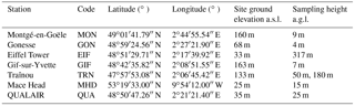
Figure 1 shows the total annual CO2 emissions emitted from IdF at the resolution of 1 × 1 km2 (AIRPARIF, 2010). As shown in Fig. 1, there is a large spatial variability of CO2 emissions in IdF which is mainly driven by the population density and the location of highways. Each year, average emissions in the center of Paris are estimated to be ∼ 70 000 t CO2 km−2 compared to ∼ 5000 t CO2 km−2 at the suburban borders. Emissions have a temporal variability on diurnal, synoptic and seasonal scales, mainly because CO2 emitted by heating varies with temperature and season, and CO2 emitted by traffic changes with the time of the day, day of the week and vacation periods (see Fig. 3, Bréon et al., 2015). Figure 1 also shows emissions from industry and energy production that come from point sources here distributed on 1 × 1 km grid cells. According to AIRPARIF, these sources are located mostly in the north and northeastern areas of Paris compared with the southern part of Paris (Lopez et al., 2013). Detailed and public information on a total of 123 point sources of CO2 in IdF can be found online for the year 2010 at the following address: http://www.georisques.gouv.fr/dossiers/irep/form-etablissement/resultats?annee=2010®ion=11&polluant=131#/. Some of these point sources are located within a few kilometers of the sampling sites as detailed in Sect. 2.1.2 and may have an impact on the observed CO2 concentration, as discussed in Sect. 3.5.2. Figure 2 shows the distribution of fossil fuel and cement CO2 emissions in western Europe extracted from the EDGAR v4.0 emission inventory (http://edgar.jrc.ec.europa.eu/, 2009), highlighting large anthropogenic emission spots in the Paris megacity, but also in the Benelux area, the Ruhr Valley and the London megacity, that may enrich the synoptic air masses with high CO2 concentrations before they reach the Paris region.
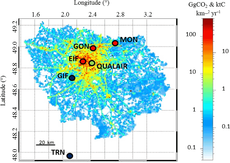
Figure 1Annual emissions of CO2 from Île-de-France at a spatial resolution of 1 × 1 km2 (AIRPARIF, 2010) and our Paris megacity CO2 in situ network: the red points indicate the CO2-MegaParis stations (MON is a NE rural site at 9 m a.g.l.; GON is a NE peri-urban site at 4 m a.g.l.; EIF is an urban site at 317 m a.g.l.); the dark blue points are stations from the ICOS-France network (GIF is a SW peri-urban site at 7 m a.g.l.; TRN is a SW rural site at 50 and 180 m a.g.l.). The QUALAIR station for monitoring the atmospheric boundary layer height in the city of Paris is also shown (green point).
2.1.2 Sampling sites
The locations of the observation sites are represented in Figs. 1 and 2. Table 1 gives their exact geographical coordinates. The sites were carefully chosen so that they would not contaminate the CO2 measurements by their own emissions.
The EIF station was installed on the highest floor accessible to tourists, in a closed room of 1.5 m2 under the stairs providing access to the tower communication antennas. To prevent contamination by the visitors' respiration, the air inlet was elevated to about 15 m above the last floor accessible to tourists, at the antenna level (317 m a.g.l.), where it was protected from uplifted air by several intermediate metallic floors. The instrument was set up in a Faraday cage to avoid interferences from strong electromagnetic radiations from the antennae. The location of the Eiffel Tower is not exactly central within Paris. The 0–180∘ (N, E and S) wind sector of the station is exposed to a larger urbanized and industrialized area than the 180–270∘ sector (S to W). In the 0–180∘ wind sector, the urbanized area covers a radius of about 20 km and includes two large point sources that are the waste burning facility of Ivry-sur-Seine (in the SE direction of the Eiffel Tower) and the heating facility of Saint-Ouen (in the north). In the 180–270∘ wind sector, the urbanized area extends barely within a 10 km radius before entering into broadleaved forests covering ∼ 2300 ha. The 270–360∘ wind sector is also mostly urbanized over a radius of about 15 km, although it comprises the woods of Boulogne (about 840 ha) which are located only 2 km NW of the Eiffel Tower.

Figure 2Location of the Paris megacity on a map of CO2 anthropogenic emissions from western Europe, adapted from the EDGAR 2009 inventory (http://edgar.jrc.ec.europa.eu/, 2009). Emissions are given in Tg of CO2 eq. per grid cell (10 × 10 km2). Some of the main emitting points in western Europe are also given. The geographical position of the remote site of MHD on the west coast of Ireland is also shown.
The GON station was set up about 20 km northeast of the Eiffel Tower at the local fire station in a residential area comprising a combination of streets and lawn gardens with a few trees around. The analyzer was hosted in a shelter equipped with a mast of ∼ 4 m standing below the canopy level (∼ 15 m a.g.l.). However, the distance from the mast to the closest trees was at least 20 m and the station was well exposed to wind from all directions. GON is located on a small hill relative to the center of Paris, and in the southerly direction, the station benefits from an open view of the city. About 3 to 4 km to the southeast and east of the station is a highway which carries high traffic during rush hours, as early as 5:00 UTC. The highway connects the center of Paris and CDG Airport, which is located about 7 km northeast of GON. The station is also close to the Bourget Airport located about 2.5 km to the south. Finally, in the W–NW sector, two noticeable industrial sources located at about 5 km from Gonesse (Fig. 1) should be mentioned as they might have an influence on the CO2 measurements (Sect. 3.5.2): a thermal plant in Sarcelles that emitted 44 kt CO2 yr−1 in 2010 and an energy production plant in Le Plessis-Gassot that emitted 128 kt CO2 yr−1 in 2010 (source: http://www.georisques.gouv.fr).
The MON station was set up in the small village of the same name with approximately 700 inhabitants located on the middle of the slope of a small hill (∼ 20 m high). The analyzer was installed on the top of the three-floor city hall building (∼ 9 m a.g.l.). The air inlet was set up on an arm pointing about 1.5 m outside of the window towards the south (200∘) opening onto fields. The north sector was covered by a few houses situated at the edge of a forest of broadleaved trees. The city hall is located on the southern side of the main road of the village which approximatively follows a northwest–southeast axis. Most of its close surroundings are agricultural fields and small villages connected by secondary roads. Montgé-en-Goële is located approximately 10 km east of CDG Airport. Two noticeable point sources are relatively close to the station (Fig. 1) and could influence the measurements (Sect. 3.5.2): a cement plant 3 km east in Saint-Soupplets (43 kt CO2 yr−1 in 2010; source: http://www.georisques.gouv.fr/) and a waste burning facility 7 km east in Monthyon (106 kt CO2 yr−1 in 2011; source: http://www.georisques.gouv.fr/). MON was considered as a NE rural site for the Paris megacity.
The GIF station, previously described in Lopez et al. (2012, 2013), has been running continuously since 2001 at LSCE (Laboratoire des Sciences du Climat et de l'Environnement). The air inlet is set up on the roof of a building at 7 m a.g.l.. The site is located ∼ 20 km southwest of the center of Paris on the Plateau de Saclay and surrounded mainly in the 0–90∘ sector by agricultural fields and by a few villages. A few hundred meters further in this direction, a national road passes on a north–south axis with high traffic levels during the morning and in the evening during rush hours. About 1 km further in the 270–360∘ sector, the atomic and environmental research agency (CEA of Saclay) holds approximately 7000 employees and is equipped with a thermal plant (17 kt CO2 in 2010; source: http://www.georisques.gouv.fr/) and that is further surrounded by agricultural fields. In the last wind sector (90–270∘), a band of forest of about 1 km depth extends along the west–east axis down to the bed of the Yvette river. A noticeable point source in the vicinity of GIF, a thermal plant located in Les Ulis, is located about 5 km further southeast (98.5 kt CO2 in 2010; source: http://www.georisques.gouv.fr/). The GIF station is located roughly at the same distance from the Eiffel Tower as GON. However, the environment is more rural in GIF than in GON so that we can label GON as a residential peri-urban site and GIF as a remote peri-urban site – although it is not as rural as the site at MON. Orly Airport is located about 16 km east of GIF.
The TRN station, previously described by Schmidt et al. (2014), has been running continuously since 2007. It is located about 120 km south of the center of Paris in the region “Centre”, within the Orléans forest (50 000 ha). A 200 m transmitter mast was equipped with four sampling levels: 5, 50, 100 and 180 m a.g.l.. TRN is located ∼ 13 km northeast of the city of Orléans which has about 120 000 inhabitants. There are a few villages around the station, including Traînou village with 3195 inhabitants in 2012 (http://www.insee.fr/fr/themes/comparateur.asp?codgeo=com-45327). The station is surrounded by agricultural fields and a mixed forest composed of deciduous and evergreen trees. In this study, we use the datasets sampled from the 50 and 180 m levels. TRN is considered as a rural site for the Paris megacity.
The MHD station has already been described by Biraud et al. (2000) and Messager et al. (2008). Atmospheric CO2 has been continuously measured there since 1992. This station, located on the west coast of Ireland, is an important site for atmospheric research in the Northern Hemisphere, as its remote location facilitates the investigation of trace constituent changes in marine and continental air masses. Most often, the station receives maritime air masses, although sometimes it is in the footprint of continental air masses coming from Europe, or more locally from Ireland and the UK (see Messager et al., 2008 for further details). In this study, MHD was evaluated as a potential background site for urban regional studies in the European continent.
The QUA station is located in the Paris city center on the campus of Université Pierre et Marie Curie in Jussieu on the top floor of a building (25 m a.g.l.), about 4 km east of the Eiffel Tower along the Seine river. It is briefly described in Dieudonné (2012). This station allows monitoring the height of the urban atmospheric boundary layer (ABL) above the Paris megacity.
2.2 CO2 measurements
2.2.1 Measurement system and calibration procedure
The CO2 datasets of the CO2-MegaParis stations (MON, GON and EIF) were collected from 8 August 2010 to 13 July 2011 using cavity ring-down spectroscopy (CRDS) analyzers (Picarro, model G1302) at 0.5 Hz. These three stations were identically set up: atmospheric air was pumped through short inlet lines made of Synflex® (4.3 mm inner diameter) with a flow rate of 0.15 L min−1. The cell temperature of the analyzers was controlled at 45 ∘C and the cell pressure at 140 Torr. At EIF, the analyzer was specifically designed to undergo higher temperatures inherent to the metallic structure of the tower and the cell temperature set point was set higher (60 ∘C). No specific impact of this set point was observed on the measurements. Air was not dried before analysis at the 3 stations and we applied the automatic CO2 water correction implemented on the CRDS instruments (Rella, 2010) to our datasets.
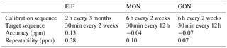
The GON and MON stations were equipped with four high-pressure aluminum cylinders containing gas mixtures of CO2 in synthetic air (matrix of N2, O2 and Ar) for instrument calibration. Before on-site deployment, the CO2 concentration of the cylinders was assigned at LSCE on the WMO-X2007 scale by a gas chromatograph (GC) described in Lopez et al. (2012). It spanned a range from 370 to 500 ppm. At each site, three of the tanks were used for instrument calibration and measured every 2 weeks. The calibration sequence consisted of four cycles (6 h total). Each cycle measured the tanks one after the other for 30 min each. The fourth tank called “target” was run for 30 min every 12 h. The target was used to monitor the instrumental drift and to assess the dataset accuracy and repeatability. At EIF, for safety reasons, it was not possible to leave any gas tanks on the site so the target tank was measured every 2 weeks and the calibration gases every 3 months only (two calibration cycles of 20 min for each gas, for a total sequence of 2 h). The instrumentation and the calibration procedure of the two SO-RAMCES stations (GIF and TRN) have already been described in Lopez et al. (2012, 2013) and Schmidt et al. (2014).
Table 2Calibration and target frequencies, accuracy and repeatability of the CO2-MegaParis stations. The accuracy is given as the difference of the target CO2 concentrations measured by the CRDS analyzer and the GC.
2.2.2 Data processing and quality control
The CRDS CO2 data were calibrated by applying a linear fit to the CO2 concentration of the calibration tanks as measured by the CRDS analyzer versus the CO2 concentration as measured by the GC. Gas equilibrium issues implied retaining only the last calibration cycle of the four cycles at MON and GON (and of the two cycles at EIF) to compute the calibration equation. For all of the calibration and target gas cylinders, the CRDS CO2 concentration was calculated as the average of the last 5 min of each gas. The accuracy of the datasets was calculated as the mean difference between the CO2 concentration reported by the CRDS analyzer and by the GC for the target gas. The long-term repeatability of each dataset was calculated as the standard deviation of the mean concentration of the target gas reported by the CRDS analyzer over the year of observations.
Table 2 summarizes the accuracy (≤ 0.13 ppm) and repeatability (≤ 0.38 ppm) calculated from the 5 min averaged data for MON, GON and EIF. As expected, the dataset of EIF shows larger deviations compared to GON and MON due to less frequent calibration and target gas measurements and a shorter calibration procedure.
The data of GON, EIF and MON were automatically filtered against cavity pressure (P) and cavity temperature (T) departure to the set points (P0 and T0) according to the ICOS procedure (Hazan et al., 2016), keeping only points for which < 0.1 Torr and < 0.004 ∘C for MON and EIF (0.006 ∘C for EIF). Furthermore, dead volumes in the setup led to instability in the response of the analyzer for 2 min after switching from one gas line to another. These 2 min periods were automatically removed from the datasets.
The data were also manually inspected to remove CO2 spikes due to very local influences (fire training at the GON station, breathing of a maintenance operator on the sampling inlet, etc.). Very local influences were identified from the short duration of the events (a few seconds to some minutes) and from the large standard deviation of the CO2 averages associated with these events. This amounted to less than 1 % of the total datasets, resulting in 91 % of the data validated after the (P, T) filtering and the manual quality control.
The GIF, TRN and MHD data processing and quality check were assessed in previous studies by Schmidt et al. (2014) and Messager et al. (2008): the repeatability of the 1 h average CO2 concentration of the target gas is 0.05 ppm at GIF, 0.06 ppm at TRN and 0.05 ppm at MHD. The instrumentation at these three sites is directly linked to the WMO-X2007 scale (Zhao and Tans, 2006).
Table 3Monthly means and standard deviation (±1σ) of the CO2 concentration (in ppm) measured at each site and data coverage of each month (in percent).
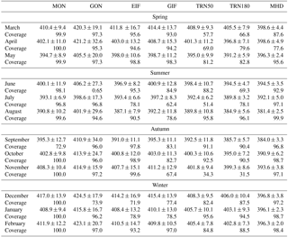
At each station, some instrument failures occurred during the period of the CO2-MegaParis study. The amount of available data points in the final datasets which are all provided as hourly averages is reported in Table 3 for each month and for each site, and is in most cases above 80 %.
In the following study, we will use CO2 hourly means for all of the stations. Apart from a few exceptions that will be identified, time is always given in UTC. Local time in Paris is UTC + 2 from April to October and UTC + 1 from November to March.
2.3 Atmospheric boundary layer height measurements
ABL heights over Paris were determined using the 532 nm elastic lidar of the QUALAIR station (http://qualair.aero.jussieu.fr/) from 8 August 2010 to 31 March 2011. A description of the instrumental setup and data processing can be found in Dieudonné (2012) and Dieudonné et al. (2013). The ABL height (ABLH) can be retrieved from elastic lidar measurements because the lidar signal is proportional to the backscattering coefficient of aerosols. In fair weather, this leads to a sharp signal decrease between the polluted boundary layer (where aerosols emitted from the surface are trapped) and the clean free troposphere. The altitude where the signal first derivative reaches its absolute minimum corresponds to the center of the entrainment zone (Menut et al., 1999). The depth of the layer where the signal first derivative is lower than 80 % of its absolute minimum is used to estimate the base of the entrainment zone, which corresponds here to the lowest ABL height (LBLH) estimate. More complex situations can occur when elevated layers of aerosols are present in the free troposphere. In that case, the absolute minimum of the signal gradient can be located other than at the top of the ABL. To resolve such situations, threshold conditions are applied to discriminate significant minima of the signal gradient (Dieudonné, 2012), and results are manually inspected to check for temporal continuity (as the altitude of a layer cannot vary much from one lidar profile to the next). When the ABL is capped by a cloud, the very strong light scattering by water droplets creates a sharp increase of the lidar signal at the top of the ABL. In such cloudy weather, the cloud base height is the best estimation for the ABLH. The LBLH is calculated as in fair weather.
The ABL height database was constructed by applying this detection method to hourly average lidar data, leading to hourly average ABL depth values. The data were acquired during daytime and weekdays, since an operator had to be on site to shut down the system in the case of rain. The dataset covers 70 % of the year of study.
2.4 Meteorological fields
Urbanized areas are characterized by specific meteorological patterns (e.g., Masson, 2000). For example, the urban heat island effect was observed to generate a gradient of temperature of a few degrees and a gradient in the ABLH of several percent between Paris city center and its rural surroundings (Pal et al., 2012; Lac et al., 2013). As far as possible, it is thus appropriate to use local meteorological fields for each of the regional atmospheric CO2 stations. Since our sites were not equipped with their own meteorological sensors, the Meso-NH model was run over the full period of study at a time step of 60 s and a spatial resolution of 2 km to generate wind speed and direction over a domain including Île-de-France (Lac et al., 2013). This modeling framework includes the land– and surface–atmosphere interaction model SURFEX with an urban scheme (town energy balance, TEB; Masson, 2000) and a vegetation scheme (Interactions between Soil, Biosphere, and Atmosphere, ISBA-A-gs; Calvet et al., 1998; Noilhan and Planton, 1989). It was already validated against observations for 1 week in March 2011 in Lac et al. (2013), where it is described in detail. The meteorological fields were extracted for the present study from the model with an output frequency of 1 h at the sampling height of each station. About 1.5 km north of GIF at the CEA of Saclay (SAC), a mast equipped with meteorological sensors provided wind field data at 10 m a.g.l. from August 2010 to April 2011. In that period, the observed SAC and the modeled GIF meteorological datasets match each other on average within 0.8 m s−1 for wind speed and 3.7∘ for wind direction, giving additional confidence in the average behavior of the model, at least in such peri-urban areas.
For wind fields at MHD, we use a local meteorological hourly observation dataset provided by Met Éireann (http://www.met.ie).
Figure 3 shows the wind roses at GIF for each season (using Meso-NH modeled data), given that the synoptic features are broadly similar to all of the regional stations. Two dominant wind regimes were observed according to the general meteorological features of the region: the southwest regime dominates mostly in summer, autumn and winter, and a northern regime (northeast and northwest sectors) mostly in spring and winter. Wind speed varied from ∼ 0 m s−1 on 18 September 2010 to a maximum of 11.1 m s−1 on 13 November 2010, the mean wind speed being 3.4 m s−1. The first (25 %) and third (75 %) quartiles were 2.2 and 4.4 m s−1, respectively. The main variations of wind speed occurred during changes of synoptic conditions. In MHD, winds blew mostly from the Atlantic Ocean in all seasons, including both the southwest and the southeast sectors. MHD also sometimes received continental air masses mostly in winter, spring and autumn. At this station, wind speeds ranged from 0.1 to 25.3 m s−1 with a mean at 7 m s−1 and the first and third quartiles at 4.1 and 9.5 m s−1, respectively.
Regarding temperature, field observations were available over the full period of study at 100 m a.g.l. at SAC (but not closer to the surface). Since we are mostly interested in relative variations of the temperature at the seasonal scale, we use this dataset as a proxy of the air temperature for all stations located in IdF (although we know that the urban heat island can generate differences of a few degrees between the city and its surroundings, as shown in Pal et al., 2012). The hourly temperature dataset collected at SAC 100 m a.g.l. over the whole period of study is shown in Fig. S2 in the Supplement. Temperature ranges from a minimum monthly mean of 0 ∘C in December to a maximum monthly mean of 18.8 ∘C in August.
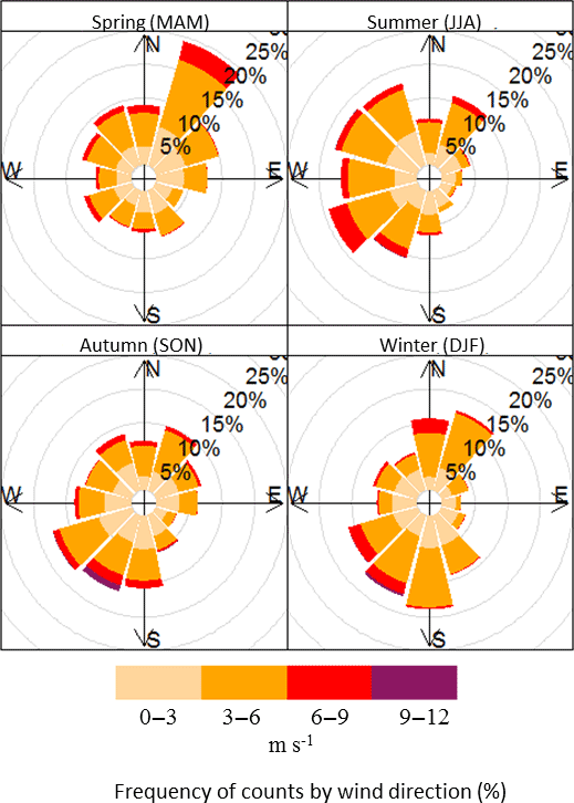
Figure 3Wind rose at GIF (7 m a.g.l., SW peri-urban site) given by season over the period of study (8 August 2010–13 July 2011) from the Meso-NH modeled wind fields. Colors indicate the wind speed according to the given scale (in m s−1).
3.1 Air mass back trajectories and wind classification of the CO2 concentration time series
In order to get information about the origin of the air masses that reached our stations, back trajectories from the Hybrid Single-Particle Lagrangian Integrated Trajectory model (HYSPLIT; https://www.arl.noaa.gov/hysplit/hysplit/) model were calculated for the city of Paris over the full period of study. We used wind fields from the NOAA-NCEP/NCAR reanalysis data archives at 2.5∘ × 2.5∘ and 6 h resolution (http://rda.ucar.edu/datasets/ds090.0/). The back trajectories were run for 72 h backwards and started at 10 m a.g.l. They were then aggregated on monthly plots that are shown in the Supplement (Fig. S1). In all cases, the monthly clusters illustrate the high variability of the origin of the air masses, which could pass over high CO2 emission areas such as the megacity of London, the Benelux or Ruhr regions before reaching IdF. The air masses could also be advected from clean areas such as the Atlantic Ocean or from biospheric regions such as in the middle of France. This high atmospheric transport variability implies that the Paris regional CO2 background signal may be highly variable depending on the synoptic conditions and that wind direction and speed are key parameters to take into account in order to understand the CO2 concentrations recorded at the different sites. The HYSPLIT model does not have a sufficient resolution to get more precise and quantitative information on the influence of local, regional and remote emissions on our CO2 observations, and getting higher resolved transport information would require a very specific (and expensive) modeling work that is out of the scope of this study. Therefore, in order to go further into the analysis, we used the modeled meteorological fields presented in Sect. 2.4 to classify the CO2 hourly time series into six wind classes (Fig. 4a and b). The local class is defined for wind speed less than 3 m s−1 and the remote class for wind speed higher than 9 m s−1. For wind speeds between 3 and 9 m s−1, we defined four remaining classes according to the wind direction: northeast (NE), northwest (NW), southeast (SE) and southwest (SW). As an example, in GIF, the partition of air masses between the different wind sectors over the full period of study is the following: 16 % from the NE, 15 % from the NW, 24 % from the SW, 7.5 % from the SE, 36 % from the local class and 1.5 % from the remote class.

Figure 4(a) Time series of CO2 concentration (1 h averages) recorded during the CO2-MegaParis period and colored by wind classed for sites MON (NE rural site, 9 m a.g.l.), GON (peri-urban site, 4 m a.g.l.), EIF (urban site, 317 m a.g.l.) and GIF (SW peri-urban site, 7 m a.g.l.). (b) Time series of CO2 concentration (1 h averages) recorded during the CO2-MegaParis period and colored by wind classed for sites TRN50 (rural SW, 50 m a.g.l.) and MHD (coastal remote site, 15 m a.g.l.).
In Fig. 4a and b, as expected, wind direction and wind speed appear to be part of the main controlling factors of the CO2 mixing ratio values recorded in the different stations. The urban and peri-urban stations are characterized by higher mixing ratios and a much larger variability than the rural and background sites. The highest variability is observed on the GON time series, followed by EIF and GIF. We note as well that the highest mixing ratios recorded at the southern rural sites (TRN50 and TRN180) and remote station of MHD occur usually during local events, likely from the influence of local emissions or remote events with northeast winds that passed over the Benelux and Ruhr areas (see back trajectories in Fig. S1 in the Supplement) and were loaded with anthropogenic emissions (Xueref-Remy et al., 2011) before reaching IdF. We also observe simultaneous variations between the sites for the local wind class: for example, peaks of the CO2 mixing ratio are observed in all the stations of IdF in mid-February and the end of March 2011, which correspond to two pollution events reported by AIRPARIF (http://www.airparif.asso.fr). However, there are some other dates (not reported by AIRPARIF as pollution events) during which the CO2 mixing ratio peaks at the urban and peri-urban stations and also sometimes at the rural stations (e.g., 20–25 August and 22–25 October). The wind classification applied on the datasets will be further used to better assess the general features of the CO2 seasonal cycles, and a much finer wind analysis will be conducted in Sect. 3.5.2 to assess the role of local, regional and remote emissions on the CO2 time series collected within the Paris observation network.
3.2 CO2 diurnal cycles
3.2.1 Mean CO2 diurnal cycles
Diurnal cycles of atmospheric CO2 are affected by local sources and sinks, regional transport and ABL dynamics (Fang et al., 2014; Garcia et al., 2010, 2012; Rice and Bostrom, 2011; Artuso et al., 2009; George et al., 2007; Gerbig et al., 2006). The mean CO2 diurnal cycles and associated 1σ standard deviation are shown in Fig. S3 for the different stations.
Noticeable differences are observed between the sites. The diurnal amplitude of the CO2 concentration from the lowest to the highest point is 2.6 ppm (MHD), 6.5 ppm (TRN180), 11.2 ppm (EIF), 14.9 ppm (MON), 15.5 ppm (TRN50), 18.2 ppm (GIF) and 30.6 ppm (GON). While the CO2 diurnal pattern at TRN can mostly be explained by biospheric activity and vertical dilution in the ABL (Schmidt et al., 2014), the peri-urban and urban stations are also expected to be strongly influenced by the diurnal cycle of Parisian anthropogenic sources. For all sites except EIF, the maximum concentration occurs in the late night/early morning (04:00–05:00 UTC for TRN50, MON, GIF and GON; 07:00–08:00 UTC for TRN180) when the ABL is the most shallow, vegetation respires and rush hours traffic occurs (05:00–09:00 UTC; source: http://www.dir.ile-de-france.developpement-durable.gouv.fr/les-comptages-a174.html). The minimum of the cycle occurs in the afternoon (14:00 to 17:00 UTC) when the ABL is the deepest and well mixed, and during seasons when the vegetation photosynthesis is active. Note that, for the case of Los Angeles (Newman et al., 2013), the annual mean CO2 concentration does not peak during rush hours, meaning that traffic is not the primary driver of the shape of the annual CO2 diurnal cycle at the Paris surface stations, nor are other anthropogenic sources, but rather the main drivers seem to be the biospheric activity and the ABL dynamics, deadening the diurnal features of anthropogenic emissions. The case of EIF is specific due to its elevation and a strong interaction of urban CO2 emissions with the ABL cycle (see Sect. 3.2.3). As a consequence, the maximum CO2 concentration at EIF occurs in the mid-morning (10:00 UTC) and its minimum is at night (00:00 UTC).
Comparing the 50 and 180 m levels at TRN, we observe a vertical gradient of CO2 concentration, along with a phase shift of the diurnal cycle: the maximum concentration is observed at 05:00 UTC at TRN50 versus 07:00 UTC at TRN180 due to the coupling of the CO2 fluxes with the ABL cycle. CO2 emitted during the night and early morning by anthropogenic sources and by the biosphere's respiration accumulates near the ground into the shallow nocturnal boundary layer (Schmidt et al., 2014) until the ABL develops in the morning, uplifting CO2 (from 05:00 to 07:00 UTC) to the 180 m level. In the afternoon, when the ABL is well mixed and deeper than 180 m, the mean difference between the concentration at the 50 and 180 m levels is very low (0.3 ppm). Furthermore, as noticed in Schmidt et al. (2014), the amplitude of the diurnal cycle decreases with increased sampling height as elevated sampling levels are decoupled from the CO2 sources during the night. As reported in Fang et al. (2014), this covariance between biospheric CO2 activities and the ABL dynamics can make it difficult for inversion models to properly reproduce the CO2 vertical gradient and thus use nighttime data for inversions. During mid-afternoon, the ABL is well mixed and the vertical bias would be very tiny.
There is a significant enhancement in the CO2 concentration observed at the regional stations compared to MHD, that increases the closer a station is to the city of Paris (apart from EIF). The difference of concentration observed between two sites depends on the time of the day, and its variation is mainly driven by the CO2 diurnal cycle at the continental sites. Apart from EIF, the more the station is surrounded by urbanization, the higher is the concentration enhancement compared to MHD, as the average levels of the CO2 concentration recorded at a station increases with a higher proximity to anthropogenic emissions from Paris. Figure 5a–g show that the hourly 1σ variability of the mean diurnal cycle remains quite constant over the day at TRN50, TRN180 and MHD. It is a bit more variable for the rural and remote peri-urban stations that are located within IdF (MON and GIF). The variability changes significantly with the time of the day at EIF and even more at GON. We can conclude that (1) the more the station is within the urbanized part of the city, the more variable is the measured CO2 signal, which reflects the spatial and temporal variability of anthropogenic emissions coupled to atmospheric transport fluctuations; and (2) the MHD signal is several ppm below the continental signals, even at the rural site of TRN that has already been shown not to be significantly influenced by the Paris megacity fluxes (Schmidt et al., 2014). Thus, MHD does not reproduce the background diurnal variability observed in the rural stations of IdF and is clearly not a relevant background site for continental European urban studies at the diurnal scale and at the regional scale of ∼ 100 km.
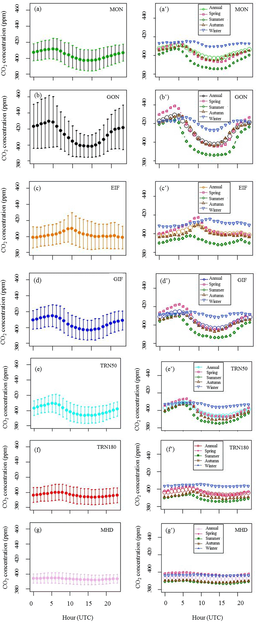
Figure 5(a–d) Diurnal cycles of CO2 from 1 h averages at (a) MON (NE rural site, 9 m a.g.l.), (b) GON (NE peri-urban site, 4 m a.g.l.), (c) EIF (urban site, 317 m a.g.l.) and (d) GIF (SW peri-urban site, 7 m a.g.l.). (a'–d') Diurnal cycles of CO2 by season at (a') MON, (b') GON, (c') EIF and (d') GIF. Note that the left and right plot scales are not the same. (e–g) Diurnal cycles of CO2 from 1 h averages at (e) TRN50 (SW rural site, 50 m a.g.l.), (f) TRN180 (SW rural site, 180 m a.g.l.) and (g) MHD (remote site, 15 m a.g.l.). (e'–g') Diurnal cycles of CO2 by season at (e') TRN50, (f') TRN180 and (g') MHD. Note that the left and right plot scales are not the same.
Figure 5a′–g′ show the mean diurnal cycle at each site by season. The influence of anthropogenic activities on the observed CO2 concentration is expected to be the highest in wintertime when emissions from heating are superimposed on traffic and other sources, photosynthesis is minimal and the diurnal ABL is thinner. Although they vary with the time of the day, on average CO2 emissions from traffic are quite constant throughout the year but they vary at the hourly and daily scales (according to the AIRPARIF 2010 inventory: on average, 1.5 kt yr−1 during weekends and 2.5 kt h−1 during weekdays, and up to 4 kt h−1 during traffic peaks; see Fig. 4 in Bréon et al., 2015). On the contrary, emissions from gas combustion (from the residential, public and commercial infrastructure that include mostly heating, production of hot water, air conditioning and cooking) show a seasonal cycle (mainly from heating), releasing about 2.5 kt h−1 of CO2 in the atmosphere in winter versus approximately 1.5 kt h−1 in summer (AIRPARIF, 2010; Bréon et al., 2015). The biospheric fluxes show large diurnal and seasonal cycles, as mentioned in Bréon et al. (2015) who reported net ecosystem exchange (NEE) outputs from the C-TESSEL model for the Paris region: NEE values are the highest in spring (−10 to −25 kt h−1 during daytime and +5 kt h−1 during nighttime, and a daily mean of −5/−10 kt yr−1 which is the same order of magnitude as fossil fuel emissions, i.e., 7 to 9 kt h−1 in spring), a bit lower in summer and autumn and much smaller in winter (−3 kt h−1 during daytime and +2 kt h−1 during nighttime, and a daily mean of −1 kt h−1, which is much smaller than fossil fuel emissions that reach 10 kt h−1 in winter). In Table S4 in the Supplement, we give for each site the annual and seasonal averages of the daily minimum and daily maximum of the hourly concentration, along with the annual and seasonal averages of the diurnal cycle amplitude (maximum–minimum concentration difference). The lines entitled “variation” give the mean of the hourly 1σ standard deviation of the minimum and maximum of each diurnal cycle.
It is noticeable that the mean winter concentration is about 6 ppm higher at MON than in TRN50. Both stations are in a rural environment, but MON is closer to Paris than TRN. As the signals are quite similar in summer, this difference can not likely be explained by the biospheric activity and is more probably partly due to a higher anthropogenic influence in MON. However, here, we need to take into account the difference of the stations inlet height (9 m a.g.l. at MON, 50 m a.g.l. at TRN50): as shown in Schmidt et al. (2014) for the 2010 winter season at Traînou, during daytime, CO2 concentrations measured at 10 and 50 m a.g.l. are similar, but this is not the case during nighttime when the CO2 concentration is about 3 ppm higher at 10 m a.g.l. than at 50 m a.g.l. because atmospheric mixing is not existent at night and CO2 sources accumulate near the surface (Denning et al., 1995). This means that the difference between MON and TRN at the inlet height of MON is of the order of 6 ppm during daytime and twice as low during nighttime. This is consistent with the hypothesis of a higher impact of anthropogenic emissions in MON than in TRN, that according to AIRPARIF are lower during nighttime than during daytime, although we do not observe the same order of magnitude (AIRPARIF gives a ratio of daytime to nighttime emissions equal to 3–4 in wintertime, while we observe a ratio of 2; see Fig. 3 in Bréon et al., 2015). Remember though that the diurnal cycle of the emission inventory is an average for the whole IdF region and not only for the MON area. The impact from local sources and/or the CO2 emission plume of the Paris megacity on MON will be further inferred from the wind analysis in Sect. 3.5.
The influence of urban emissions in GIF, MON and GON results in a higher mean diurnal concentration of atmospheric CO2 at these sites compared to the others for all seasons (and mainly in winter) and of its variability. The impact of traffic emissions is well visible in GIF, MON and GON in the winter season only with two CO2 maxima during rush hours (morning and evening). Although traffic occurs throughout the year, these peaks are likely more or less masked by the biospheric activity and the ABLH dynamics during the other seasons (see above). In addition, the ABL is shallower during winter leading to higher CO2 concentrations. The amplitude of the morning and evening peaks is higher in GON than in GIF and MON, and denotes a stronger impact of traffic emissions in GON than in the two other stations. GON also shows the maximum interseasonal difference between summer and winter (31.3 ppm in the afternoon) which is higher than the mean annual afternoon dispersion, meaning, in other terms, that the seasonal variability is higher than the mean annual dispersion of the fluxes in the afternoon. Actually, the whole diurnal cycle is shifted towards higher concentrations at GON, the mean concentration being higher in GON than in GIF, TRN50, TRN180 and MHD for all seasons, with the largest differences in winter. The full variability observed at GON over the year can thus be explained partly by the seasonal variation of biospheric activity and ABL dynamics but also by a strong impact of anthropogenic CO2 emission variability. The impact of the Paris emissions versus more local sources around the station (highways, airports, heating, industrial facilities, etc.) will be further assessed in Sect. 3.5.
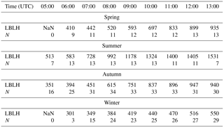
Table 4Mean altitude of the lowest estimate of the boundary layer height (LBLH) by season in the morning and early afternoon (hours are given in UTC; altitude in m a.g.l.). The number of points used to calculate the means are also given (N). NaN indicates no available data.
3.2.2 The specific case of the top of the Eiffel Tower
In all seasons, the CO2 diurnal cycle at EIF is out of phase with the other stations, with a maximum occurring later, in the mid-morning instead of the late night/early morning (Figs. 5 and S3). EIF is significantly higher (317 m a.g.l.) than TRN180 (180 m a.g.l.) so when comparing these elevated sites to ground stations, the effect of the CO2 coupling with the ABL dynamics can be expected to appear stronger at EIF than at TRN180. Such coupling was already mentioned in the framework of a direct CO2 transport modeling study in March 2011 (Lac et al., 2013). Furthermore, Dieudonné et al. (2013) demonstrated the existence of a vertical concentration gradient between the bottom and the top of the Eiffel Tower for NO2, a species co-emitted with CO2 during combustion processes especially by the traffic sector, and this vertical gradient was shown to be correlated with the ABL dynamics.

Figure 6Diurnal cycles of the hourly LBLH estimate means (in black) ±1σ standard deviation (in grey) and of the CO2 hourly means (in red) observed by season at QUALAIR (urban site, 25 m a.g.l.) and EIF (urban site, 317 m a.g.l.), respectively. Time is in UTC. The blue horizontal line is the elevation of EIF. The violet circles give the CO2 concentration (according to the red scale) at the same moments when the LBLH (in black) was measured.
We show in Sect. S5 in the Supplement the hourly means of the LBLH observed at the QUALAIR station during daytime, colored by hour and compared with the level of the EIF station. These data are summarized in Table 4. We recall that the LBLH dataset does not cover the whole period of study but the most interesting parts of it, as it includes the cold months during which the LBLH and dynamics are at their lowest. The period of August to March allows us to observe a large portion of the seasonal cycle of the LBLH which is characterized by a change in its maximum value (on average, 1200 m in summer, 400 m in winter) and in the phase of its development, which starts earlier in summer. We do not have the proper data to quantify precisely this starting time; however, we note that the LBLH is always above the level of EIF in summer, while it is below it (at 301 m on average) before 06:00 UTC in winter (see Table 4). We can thus infer that the EIF station could be often above the nocturnal layer at night, inside the residual layer (but not in the free troposphere).
In Fig. 6, we show the CO2 diurnal cycle for each season computed using only the data that were collected at the EIF station at the same time as the LBLH data. The CO2 signal increases in the morning when the growing ABL brings to EIF the nighttime and early morning CO2 emissions that got trapped into the nocturnal and/or nascent boundary layer. However, compared to TRN180, the effect at EIF is much stronger due to larger emissions in the city, especially from the morning traffic peak (from 06:00 to 10:00 UTC, i.e., 04:00–08:00 UTC in summer and 05:00–09:00 UTC in winter) (http://www.dir.ile-de-france.developpement-durable.gouv.fr/les-comptages-a174.html). Later, the CO2 signal dilutes into the growing ABL to reach a minimum in the afternoon.
Autumn. The LBLH is close to the EIF altitude. The moderate development of the ABL during the morning does not compensate for the accumulation of the peak traffic emission in the ABL, so that the CO2 concentration increases from 05:00 to 10:00 UTC, leading to a CO2 increase of 17.1 ppm for an LBLH increase of 470 m. At the end of the afternoon, the LBLH decreases and it gets close to the level of EIF, decoupling the station from the surface. This could explain why the late night/early morning concentrations are relatively low and the morning bump of CO2 quite large. However, this remains a hypothesis as we do not have enough points for a robust demonstration.
Winter. As expected, the process of vertical mixing is quite slow in wintertime. The CO2 concentration increases in the morning (∼ + 6 ppm) with the maximum concentration encountered at 13:00 UTC for a development of the LBLH of only ∼ 157 m within a 7 h time frame. After the morning flush of the surface emissions due to the growth of the ABL, the concentration decreases quite rapidly to reach its daily minimum at 16:00 UTC. At the end of the day, the LBLH falls and gets quite rapidly below the EIF station level, decoupling the EIF station from the surface. Although we do not have lidar data after 18:00 UTC to confirm it, this likely explains the relatively low level of CO2 concentrations observed late at night.
Spring. In spring, the CO2 signal increases until 10:00 UTC to a maximum of 420 ppm while the ABL height increases by ∼ 287 m. The shape of the CO2 mean concentration and LBLH diurnal cycles suggests that the relatively high CO2 concentrations encountered in the late night/early morning result from the evening high CO2 emissions trapped in the previous day's ABL that became the residual layer at night.
Summer. The CO2 concentration is on average lower than in the other seasons due to local and regional photosynthesis activity, lower anthropogenic emission levels and higher LBLH. In particular, the observed LBLH during daytime is always above the EIF station level (Fig. S5) so that one would expect CO2 concentrations to peak in phase with the traffic counter records, between 06:00 and 07:00 UTC. However, the CO2 diurnal cycle at EIF remains out of phase with those recorded at ground-level stations, though the delay with the morning peak is reduced compared to other seasons. The CO2 concentration remains quite stable between 07:00 and 09:00 UTC, despite the increasing LBLH (+460 m) and the decreasing traffic counts. However, one must keep in mind that until late morning, the air dragged into the ABL by entrainment does not come from the clean free troposphere but from the polluted residual layer, explaining why high CO2 concentration can maintain. After 09:00 UTC, the CO2 concentration steadily decreases, though the average LBLH still increases. This drop in concentration can be explained both by an increase in the photosynthetic activity with increasing solar flux and by vertical dilution. Indeed, though the LBLH still rises after 10:00 UTC, the entrainment zone continues to grow until the mid-afternoon (Dieudonné, 2012), blending in clean air from the free troposphere. During the late afternoon, the CO2 concentration increases again as vertical mixing decays and as the evening traffic peak starts (around 15:00 UTC).
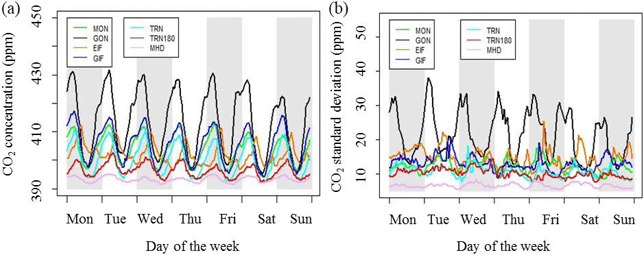
Figure 7(a) CO2 diurnal cycle by day of the week at the different stations, calculated from CO2 hourly concentrations over the whole period of study. (b) Standard variation (1σ) of the hourly CO2 mean concentration.
This analysis confirms that the coupling of the urban CO2 emissions together with the dynamics of the ABL height is very likely a major controlling factor of the specific CO2 diurnal pattern observed at EIF. We lack data at night and in the early morning to make a deeper analysis of the ABL dynamics and especially of the role of turbulence on CO2 variability. We conclude that a vertical and fluctuating gradient of CO2 likely exists above the Paris megacity, between the ground level and 317 m a.g.l. (and likely higher). Quantifying such vertical gradients is of interest since they have to be correctly reproduced in urban mesoscale modeling frameworks for accurate atmospheric CO2 inversion purposes. This vertical gradient can be roughly estimated by subtracting the EIF signal from the GON or the GIF signal. In the early morning (04:00–05:00 UTC), the GON-EIF (respectively, GIF-EIF) gradient is +35 ppm (+18 ppm) in spring, +31 ppm (+17 ppm) in summer, +30 ppm (+10 ppm) in autumn and +14 ppm (+4 ppm) in winter. In the afternoon (14:00–16:00 UTC), the GON-EIF (respectively, GIF-EIF) gradient is lower in absolute values and changes of sign: −7 ppm (−8 ppm) in spring, −4 ppm (−3 ppm) in summer, −4 ppm (−7 ppm) in autumn and −2 ppm (−5 ppm) in winter. The gradient is thus at its maximum at night and in the warm seasons, which may also reflect the influence of the biospheric respiration at the stations close to the ground level, compared to EIF. In the future, we plan to equip the Eiffel Tower with two supplementary levels of sampling to collect observations that will allow us to well characterize the CO2 vertical profile over the city of Paris and its temporal variability, and its relation with ground emission variations and their coupling with atmospheric dynamics.
3.3 Weekday versus weekend
According to the AIRPARIF inventory, the total CO2 emissions of IdF are lower during weekends than during weekdays, with mean differences of the order of 30–40 % during daytime and 50–60 % during nighttime. We infer here the impact of such variations on the atmospheric concentrations. In Fig. 7, we show the mean diurnal cycles of the CO2 concentrations at each site for each day of the week, as well as the associated standard deviation (1σ).
In GON, the CO2 concentrations are systematically lower over the weekend, especially on Sundays (5–10 % decrease during daytime, 25–35 % decrease during nighttime). A similar pattern is observed for MON. The weekdays-to-weekend ratios observed for the CO2 concentrations are lower than those computed from the emissions given by the inventories. This could be due to an overestimation of the difference from the inventory; however, biospheric fluxes (e.g., Schmidt et al., 2014), wind speed and direction (see Sect. 3.5), and CO2 background signals (see Sect. 3.1 and Turnbull et al., 2015) are also factors that modulate the observed CO2 concentration at each site. Disentangling the role of each of these factors on the differences between the observed weekdays-to-weekend CO2 concentration ratios and the ones calculated from the inventory would require a dedicated analysis that is outside the scope of this paper. Note that while the variability of the CO2 means is very large in GON, it is lower during weekends than during weekdays. The CO2 diurnal cycle does not change much in GIF between a working weekday and a weekend (except for a small decrease during nighttime over the weekend), nor at EIF and TRN, possibly because of a larger influence of the biospheric fluxes (that do not depend on weekdays or weekends) at these stations compared to the contribution of anthropogenic emissions (that are different on weekdays and weekends according to AIRPARIF; see Fig. 4 in Bréon et al., 2015) and that are the strongest observed at GON (Sect. 3.2.1 and 3.5.2). During nighttime, at GIF, we observed the highest concentrations from Sundays to Wednesdays, with concentrations lower by 3–5 ppm (a 20–25 % decrease) from Thursdays to Saturdays. This could be due to a specific traffic pattern within the footprint of the station, but we currently do not have access to local traffic data for each day of the week to verify this hypothesis.
3.4 CO2 seasonal cycle
We computed the seasonal cycle of CO2 at each site, based on the monthly means of our ∼ 1-year datasets and including all hours of the day (Fig. 8a). The seasonal cycles of the air temperature and available LBLH data (at QUA) are also shown on the same figure.
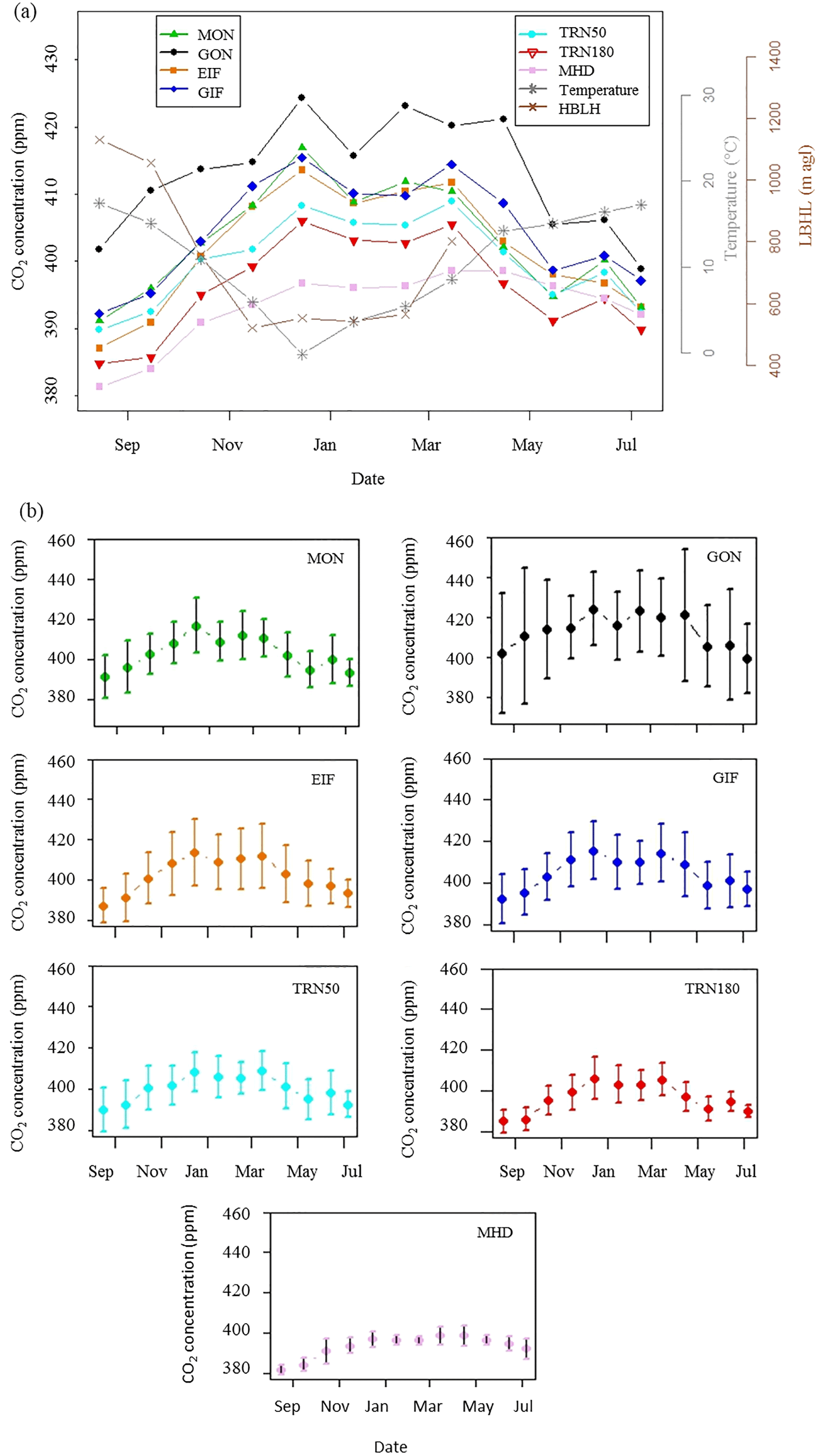
Figure 8(a) Seasonal cycles of CO2 concentration at the six sites based on monthly means. Monthly averages of air temperature at 100 m (Saclay tower near GIF) and of the LBLH (QUALAIR urban site, 25 m a.g.l.) are also shown. Note (in m a.g.l.): MON is at 9 m (NE rural site), GON is at 4 m (NE peri-urban site), EIF is at 317 m (urban site), GIF is at 7 m (SW peri-urban site), TRN50 is at 50 m (SW rural site), TRN180 is at 180 m (SW rural site), MHD is at 15 m (remote site). (b) Seasonal cycle (August 2010–July 2011) of CO2 at each of the Paris regional sites and at MHD, calculated from CO2 monthly means of hourly averages, with error bars showing 1 standard deviation ( ± 1σ) of the CO2 means. Note (in m a.g.l.): MON is at 9 m (NE rural site), GON is at 4 m (NE peri-urban site), EIF is at 317 m (urban site), GIF is at 7 m (SW peri-urban site), TRN50 is at 50 m (SW rural site), TRN180 is at 180 m (SW rural site), MHD is at 15 m (remote site).
Ignoring the specific case of EIF (Sect. 3.2.3), throughout the year we observe that the monthly mean CO2 concentration increases with the vicinity of the station to larger CO2 emission sources. The maximum CO2 enhancement compared to MHD is observed at GON which is our most anthropogenically influenced station (from 6.8 ppm in July to 27.5 ppm in December). Similarly to what is observed at the diurnal scale (Sect. 3.2), differences of several ppm are also observed between our rural sites and MHD, while the differences between the rural/peri-urban/urban stations in IdF are of the same order of magnitude. These differences of concentration between the stations located in IdF and MHD vary with the season, the seasonal cycle being much more well defined in the Paris rural stations than in MHD due to a higher biospheric activity in the IdF region than on the western coast of Ireland. This implies that background values of CO2 in IdF (i.e., without the impact of Paris emissions) should be defined at the regional scale near Paris (∼ 100 km) and not at the continental scale in MHD. Furthermore, in Sect. 3.1, we explained that the CO2 concentration fluctuates with the origin of the air masses that can be very variable, and therefore specific regional background should be selected in function of the wind direction, as also mentioned for the case of Indianapolis (Turnbull et al., 2015). In conclusion, MHD appears not to be relevant as a background site for defining the atmospheric plume of CO2 in the Paris region at the seasonal scale as well. Regional background stations (∼ 100 km) seem to be much better suited for urban regional studies in Paris and elsewhere in the European continent. Several methods are available to extract a background signal from a time series (e.g., Ruckstuhl et al., 2012; Ammoura et al., 2016). Quantifying precisely the Paris background signals values as well as the Paris plume and its variability requires a dedicated analysis that is outside the scope of the present paper: it will be specifically addressed within another dedicated study. At each station, the monthly mean CO2 concentration follows a seasonal cycle that reaches its maximum in winter and its minimum in summer. This is expected due to (1) the seasonal cycle of the biosphere; (2) the variability of anthropogenic emissions, mainly from the heating sector, which are directly linked to ambient temperature (see Sect. 3.2.2); and (3) the seasonal cycle of the ABL height (Sect. 3.2.3), which is the lowest in wintertime (e.g., Denning et al., 1995; Turnbull et al., 2009). It is difficult to estimate the biases due to missing data points in the time series (Sect. 2.2.2); however, as an indicator of robustness, the data coverage for each month and each station (given in Table 3) is very good overall.
To assess the variability of the seasonal cycle, Fig. 8b shows the CO2 monthly means at each station with error bars representing the associated 1σ standard deviation. Note that the 1σ dispersion is the highest at GON and the lowest at MHD. More generally, the variability increases with the level of urbanization around the station and the distance to anthropogenic CO2 emission sources. Therefore, increases in the variability from one month to the next can be used to track down the influence of more local and thus fresh sources, as a complement to the “local” wind sector (wind speed < 3 m s−1). Some specific seasonal patterns can be observed.
Winter. In winter, the lower biospheric activity makes the CO2 concentration relatively more sensitive to anthropogenic emissions (see Bréon et al., 2015). In Paris, January is usually the coldest month (meaning the month with the highest heating emissions). However, the months of December 2010 and February 2011 were characterized by cold episodes, while January 2011 was rather mild. This resulted in higher CO2 concentrations in December and February than in January for MON and GON. In GIF, EIF and TRN, the secondary maximum (February) is shifted to March. Indeed, in February, southerly winds prevailed (see Fig. S1 in the Supplement and also Fig. 4a and b), bringing Parisian anthropogenic CO2 emissions in the direction of GON and MON, and depleting the southern stations, while in March, winds blew mostly from the NE/SE sectors, bringing higher CO2 levels to GIF, TRN, EIF and also MHD. The higher CO2 concentration encountered in December compared to February or March can be explained by the ABL height being minimal in December (Fig. 8a). However, in February, the GON signal remains the highest of all stations, and the concentrations observed at MON are higher than those recorded at TRN. Here, we may see the impact of air masses advected from the NE with higher CO2 background levels and especially a sensitivity to upwind emissions at GON. Such influence of meteorological conditions on the seasonal cycle of continental stations was also reported in the literature (e.g., Fang et al., 2014; Zhang et al., 2008) and will be further assessed in Sect. 3.5.2.
Spring. Starting in April, we observe a decrease of CO2 at all stations except GON, as regional photosynthesis activity develops (Bréon et al., 2015). In April, the high variability of the GON signal and the prevailing local, SW and NW wind sectors show that the station experiences strong influence from anthropogenic emissions, local or advected, and explains why the CO2 concentration remains higher than at the other stations. From April to July, we observe that the CO2 concentration at TRN180 is always equal to or below MHD, showing the strong influence of regional biospheric activity on concentrations measured at continental stations. Indeed, this effect is also observed in TRN50 and MON in May when the biosphere was very active and winds blew mostly from the SE and SW, bringing air masses from the forests of the Centre region to IdF. During other spring and summer months, concentrations at TRN50 and MON remain higher than at MHD as the dominant winds were from the NE sector, likely bringing emissions from the Ruhr/Benelux areas to MON and TRN and/or from Paris to TRN.
Summer. For all stations except GON, the annual minimum of concentration is observed in August when the following occurs: (1) the minimum of anthropogenic emissions as given by the AIRPARIF inventory (see Fig. 3 in Bréon et al., 2015); (2) the maximum of photosynthetic activity (see Fig. 4 in Bréon et al); and (3) the maximum development of the ABLH (Fig. 8a). In GON, the contribution of the local wind sector is strong in August, as confirmed by the large 1σ deviation, explaining why the minimum of concentration is shifted to July, another month with reduced economic activity and emissions (on top of a high level of photosynthesis and a relatively high ABLH). The higher concentrations in August at GON are also associated with slow winds blowing from the northwest direction, indicating an impact of relatively local emissions, possibly of the two point sources mentioned in this wind sector in Sect. 2.1.2.
Autumn. September is characterized by an increase of the monthly mean CO2 concentrations at all stations, although the increase is higher in GON (+9 ppm) than elsewhere (+3 to +5 ppm). As there were several local and NW events during that month, we infer that this larger increase is due to urban emissions in the vicinity of GON (e.g., from CDG Airport) or a bit further to the NW side of GON (among which the two industrial sites mentioned in Sect. 2.1.2).
The sensitivity of the stations to wind speed and direction, and especially the question of higher background CO2 levels advected from the NE sector, will be analyzed in more detail in the next section.
3.5 Wind study: from local to regional signals
3.5.1 Wind speed effect
Wind speed is a key factor in modulating the dispersion of CO2 emissions (e.g., Idso et al., 2002; Moriwaki et al., 2006, Rice and Bostrom, 2011; Garcia et al., 2010, 2012; Lac et al., 2013; Turnbull et al., 2015). Figure 10 shows the mean hourly CO2 concentrations and the associated standard deviations recorded at GON over the year of study for local afternoon hours only (11:00–15:00 UTC) as a function of the wind speed and colored by wind direction. The CO2 concentrations have been seasonally adjusted to avoid biases due to seasonal variability (Sect. 3.4), by applying the following treatment to the CO2 hourly dataset of each station: (1) computing the annual mean of the dataset; (2) computing the monthly seasonal index for each month by calculating the ratio between the monthly mean and the annual mean of the dataset; (3) interpolating the monthly seasonal indexes at an hourly scale over the full period of study; and (4) dividing the CO2 hourly dataset by the hourly seasonal index. Figure 9a shows that the amplitude of the CO2 concentration range and especially the maximum values decrease exponentially with wind speed because of the ventilation and dilution effects. Such behavior is observed at all the regional stations, although the wind speed maximum is higher at TRN (∼ 11 m s−1) and even higher at EIF (∼ 20 m s−1) due to the elevation of these stations. The 1σ dispersion from the hourly means (called variability in Fig. 9b) shows a similar dependency on wind speed. At low wind speed, the relatively high level of variability can be associated with the impact of fresh and regional anthropogenic CO2 emissions. For high wind speeds, the hourly averaged CO2 concentration converges towards a mean value and the 1σ variability drops below 1 ppm. Such behavior was previously reported at former CO2 urban stations for other cities (e.g., Garcia et al., 2010, 2012; Rice and Bostrom, 2011; Massen and Beck, 2011). However, and contrary to those studies, we do not think that this mean value can be considered as an asymptote, as it originates only from a few sparse events (spread over 7 days of the period of study), nor that it can be considered as a background CO2 concentration for the stations.
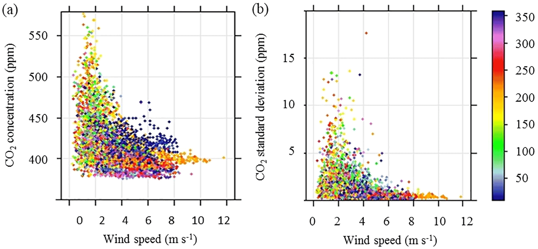
Figure 9(a) Hourly means of the CO2 concentration recorded at GON (NE peri-urban site, 4 m a.g.l.) as a function of wind speed and colored by wind direction (the color scale is in degrees). (b) Same for the CO2 standard deviation (1σ of the hourly CO2 concentration means).
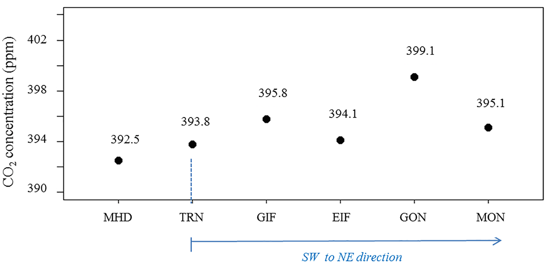
Figure 10Mean CO2 concentration (in ppm) observed at the different stations of the Paris regional network (TRN represents the measurements at 50 m a.g.l.) and at MHD for wind speed higher than 9 m s−1 over the period of study (8 August 2010–13 July 2011). During such events, the synoptic conditions were mostly oceanic (wind blowing from the SW sector). Note (in m a.g.l.): MON is at 9 m (NE rural site), GON is at 4 m (NE peri-urban site), EIF is at 317 m (urban site), GIF is at 7 m (SW peri-urban site), TRN50 is at 50 m (SW rural site), TRN180 is at 180 m (SW rural site) and MHD is at 15 m (remote site).
Figure 10 shows this CO2 mean value at the different stations: a CO2 horizontal enhancement appears as stations get closer to the city of Paris (apart from EIF), with the maximum difference (6.6 ppm) observed between GON and MHD. The high wind speed events that occurred during the period of study correspond only to winds blowing from the southwest, mostly from the 200–220∘ sector. GON was thus immediately downwind of Paris emissions, most likely the reason why it exhibits the highest mean constant value. An enhancement is also observed at TRN and at GIF compared to MHD. As both TRN and GIF are located upwind of Paris, we see once again here that MHD does not provide an adequate CO2 concentration background level for Paris and other continental western European cities. The peri-urban upwind station of GIF has quite a similar mean constant value to the rural downwind station of MON. Indeed, MON station was not in the path of Paris CO2 urban plume in this 20∘ wind sector. The EIF value is also lower than at GIF and GON, supporting the fact that for such high winds, the top of the Eiffel Tower was not very sensitive to surface emissions, most likely because between 0 and 300 m a.g.l. ventilation of emissions was stronger than their vertical mixing.
3.5.2 Fine wind sector analysis
In order to distinguish the relative contributions of the local, remote and Paris megacity regional CO2 fluxes to the CO2 concentration observed at the five stations of the Paris network, we analyzed the dependence of the observed CO2 concentration and its variability on the horizontal wind speed and direction. Considering the diurnal variability of vertical transport dynamics (Sect. 3.2), we separately analyzed afternoon (11:00 to 15:00 UTC) and nighttime (22:00 to 02:00 UTC) data. For the TRN station, we consider that the TRN50 level is sufficient for this analysis.
Inner Paris extends to a diameter of 10 km, while the Paris metropolitan area extends to a diameter of 30 to 50 km. The distance of the peri-urban stations GON and GIF to the Paris inner city is about 10 and 15 km, respectively. The distance of the rural stations MON and TRN to inner Paris is about 30 and 100 km, respectively. Taking into account these distances, we set the hypothesis that we can assess the influence of local emissions using hourly means observed in low wind speed conditions (less than 3 m s−1) while the influence of remote emissions can be analyzed using data recorded in relatively high wind speed conditions (more than 8 m s−1). This relies on considering the time given for atmospheric mixing of local and regional emissions (dominant at low to moderate wind speeds) versus their ventilation (dominant at high wind speeds): the integration of local and regional emissions into an air mass, which carries the signature of remote emissions when it is upwind of Paris, gets higher with decreasing wind speeds. For example, for wind speeds lower than 3 m s−1 (11 km h−1), it takes 1 h or more for any air mass to flow over the center of Paris (∼ 10 km of diameter), allowing some time for local emissions to get mixed into the air mass, while at 8 m s−1 or more (∼ 29 km h−1) it takes about 20 min or less, allowing less time for the atmospheric integration of local to regional emissions. In the middle range of wind speed (3–8 m s−1), we expect most of the CO2 variability to be driven by the influence of the regional emissions coming from Paris.
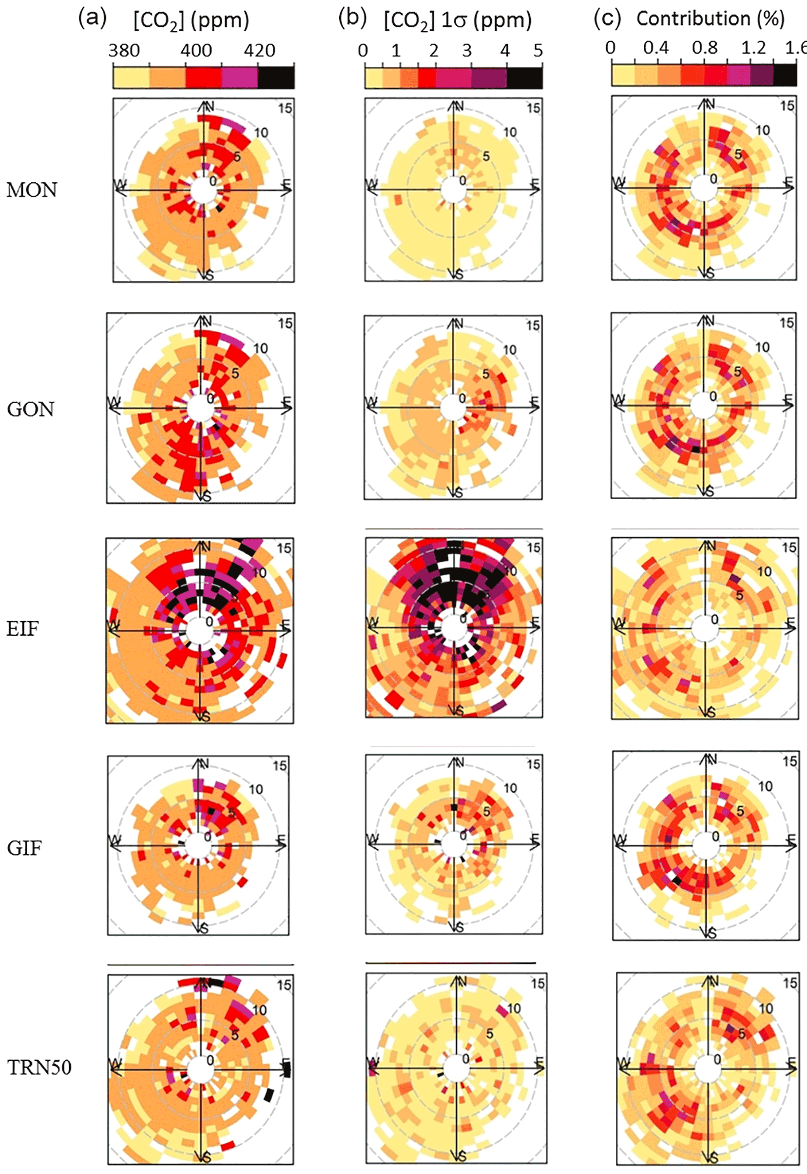
Figure 11(a) CO2 mean concentration as a function of wind speed (circles in m s−1) and wind direction at MON (NE rural), GON (NE peri-urban), EIF (urban), GIF (SW peri-urban) and TRN50 (rural) stations using daytime data (11:00–15:00 UTC) for the period of study (4 August 2010–11 July 2011). (b) Mean 1σ CO2 variability of each concentration (ws, wd) point. (c) Occurrence as the frequency of the (ws, wd) bin weighted by the square root of the CO2 concentration mean.
For all of the regional stations, Fig. 11 shows the pollution roses of the mean afternoon CO2 concentration binned by wind speed (ws) and wind direction (wd) with a resolution of 1 m s−1 for ws and 10∘ for wd. We use here the CO2 hourly concentration dataset that has been seasonally adjusted (Sect. 3.5.1). In order to assess the representativeness of each (ws, wd) bin, the contribution of each concentration mean for a given (ws, wd) bin on the total concentration is also calculated, after applying a square root transformation on the CO2 concentration to reduce any bias from the highest CO2 values (we used the polarFreq function from the OpenAir work package for R with the option “weighted mean”; more information can be found online here: http://www.openair-project.org/PDF/OpenAir_Manual.pdf). We also show the mean 1σ standard deviation of the CO2 concentration at each bin. A similar figure for nighttime data is given in Sect. S6a in the Supplement. During daytime (nighttime), the color scale is limited to the 380–430 ppm interval for the CO2 concentration and to the 0–5 ppm range for the standard deviation. There are a few values outside of these ranges that are forced to the closest range bound value. To facilitate the comparison between the stations, the highest complete wind speed circle visible on the plots is set at 10 m s−1 in all cases. For MON, GON and GIF, all the data are plotted when taking this wind speed threshold. For TRN and EIF, wind speeds can reach higher values due to the elevation of these stations (during the afternoon, up to 15 m s−1 at TRN and 25.5 m s−1 at EIF; at night, up to 15 m s−1 at TRN and 22 m s−1 at EIF). Although they represent only a minor fraction of the datasets, some of the TRN and EIF data are thus not apparent in Fig. 11: the plots for the full wind speed ranges encountered at EIF and TRN are given in Sect. S6b (daytime) and S6c (nighttime) in the Supplement.
Influence of remote emissions (> 100 km)
The back trajectories (Fig. S1 in the Supplement) show that Paris was exposed to a range of synoptic air masses over the period of study, including clean oceanic ones and others with CO2 enriched by remote anthropogenic emissions especially from Benelux, the Ruhr area and the London megacity. Relatively high CO2 concentrations (> 410 ppm) were observed for high wind speeds (> 8 m s−1) in the 0–45∘ NNE sector at the three stations located relatively close to the ground level (MON, GON and GIF). For the elevated stations (EIF and TRN), such concentration values also occur, but as expected at higher wind speeds (> 12–14 m s−1), reaching at least the 410 to 420 ppm range at all of the stations. The fraction of data falling in these (ws, wd) bins is large enough to consider these high concentration values to be statistically representative. Furthermore, the standard deviation of the signal at the upwind stations is quite low (less than 0.6 ppm), which indicates that the high concentration values observed upwind of Paris (GON and MON) are not associated with fresh emissions but with imported pollution that was already well mixed in the atmosphere. It is likely that we see here the signature of remote anthropogenic CO2 emissions from hot spots such as the Benelux and the Ruhr areas that bring higher CO2 background levels to all the stations. The high CO2 concentrations observed in the 0–35∘ NE sector at the downwind stations (EIF, GIF and TRN50) for moderate to high wind conditions (≥ 3 m s−1) appear thus to be due not only to the Paris CO2 emission plume but also to enriched background CO2 levels advected from the NE. By comparison, the background levels that are observed in the 200∘ (SE) to 280∘ (NW) sector of GIF and TRN50 are lower than 400 ppm, while the 0–35∘ NE background levels at GON and MON are often above 400 ppm, reaching concentrations in the 410–430 ppm range. This shows that the Paris megacity background values can vary by several ppm depending on the wind direction, with the highest CO2 concentrations advected in the 0–45∘ wind cone. We note also that EIF shows higher concentrations in the 295–360∘ NW sector at high wind speeds that could be associated with long-range transport of anthropogenic plumes from the northern hot spot emissions mentioned and better seen at this elevated station. Also, TRN shows higher CO2 concentrations in the 345–360∘ NW sector for high wind speeds, which could be attributed to these hot spots – but also to Paris.
During nighttime, for wind speeds higher than 8 m s−1, all stations show higher CO2 levels in the 0–45∘ NE sector than in the other wind directions (see Fig. S6a).
Influence of local emissions (< 10 km)
In Sect. 3.2.1, we questioned whether MON was under the strong influence of local signals. The MON CO2 wind rose shows that for wind speeds in the 0–2 m s−1 range, higher CO2 concentrations (400 ppm to more than 430 ppm) are observed in different wind sectors. Note that the 230–240∘ SW sector is where the bin contribution is the highest (∼ 0.8–1 %). These higher CO2 concentrations can most likely be attributed to the influence of the point sources relatively close to MON mentioned in Sect. 2.1.2 but also to relatively close diffuse emissions (traffic, heating, etc.) from ground activity under the path of the air mass and also possibly to aircraft emissions. Montgé-en-Goële is located in the path of aircraft departing from CDG for easterly winds and aircraft arriving to that airport for westerly winds (http://www.advocnar.fr/aviation-civile/flux-de-trajectoires/). The CDG platform is equipped with two runways (north and south) from which the planes both take off and land along two west–east axes and pass very close to the station at altitudes between 0 and 1000 m a.g.l.. The NW and SE sides of the station are exposed to aircraft flying, respectively, to and from the CDG northern runway, while the 260–360∘ sector and the 180–260∘ sectors are the most exposed to aircraft traffic from the southern runway. Tarmac and in-flight aircraft traffic (below 915 m a.s.l.) are estimated to represent ∼ 60 % of the airport emissions (ADP, 2013). Apart from road traffic emissions to and from CDG, the airport infrastructure itself (building heating, stopover airplane electricity supply, etc.) could also influence the station (as it represents ∼ 11 % of the airport CO2 emissions; ADP, 2013), although more likely at the regional scale (see below). A much weaker influence of the Le Bourget aircraft flight paths, passing a few kilometers further south than CDG airplanes but also at low altitude, is also possible on the southern side of the station.
In Sect. 3.2.1 and 3.4, we questioned the influence of local sources on GON (such as CDG and Le Bourget airports) but also of point sources mentioned in Sect. 2.1.2 and diffuse sources around the station. As for MON, all these types of sources in the vicinity of GON will likely influence it at low wind speed. GON is also exposed to aircraft emissions as it lies close to the lowest flight paths (0–1000 m a.g.l.) from the CDG and Le Bourget airports (http://www.advocnar.fr/aviation-civile/flux-de-trajectoires/). These emissions are due to (i) in the NW sector, takeoffs from the CDG northern runway; (ii) in the SW sector, takeoffs from the CDG southern runway and from the Le Bourget runway; (iii) in the NE sector, landing on both CDG runways; and (iv) in the SE sector, landings on the southern runway of CDG and to a lesser extent in Le Bourget Airport. Also, it is likely that GON gets exposed to emissions from the two airports themselves, located a few kilometers away. Note that the standard deviation which is more that 1 ppm higher from 60∘ (NE) to 170∘ (SE) seems to indicate fresher emissions in this wind sector. Nearby highways (located about 1.2 km north and east) could contribute in these wind directions. Discriminating between the different emission sources influencing the GON or the MON stations at low wind speed would require dedicated fine-scale modeling studies that are outside the scope of this study.
At EIF, the influence of local emissions is expected mostly between the late morning and the late afternoon since, as we have seen in Sect. 3.2.2, the top of the Eiffel Tower receives surface emissions in this time period during all seasons. The CO2 pollution rose of Fig. 11 indicates high concentrations (400 to more than 430 ppm) in all directions around the stations for wind speeds comprised between 0 and 2 m s−1. The variability is quite large (1.5 to 5 ppm), indicating fresh emissions and reflecting the spatial and temporal variability of the emissions coupled to atmospheric transport variations. Carbon isotopes and CO2 co-emitted species measurements would be useful here to estimate the role of the different emission sectors (e.g., Lopez et al., 2013; Pataki et al., 2009).
In GIF, a few high CO2 spikes are observed for low wind conditions in diverse wind directions. These spikes are likely due to emissions from traffic and heating from the surrounding infrastructure, as observed from the corresponding relatively high standard deviation (> 5 ppm). Flight paths to and from Orly Airport for westerly winds pass several kilometers south of the station and likely have a weak local impact.
Similarly to what is observed at GIF, higher CO2 concentrations are observed at TRN50 in the wind sector of the city of Orléans, located ∼ 13 km SW of the station.
At night, MON and GIF show a higher local influence that still remains moderate. At EIF, no specific local influence is observed apart from a couple of (ws, wd) bins, confirming that the station is quite disconnected from the surface where urban emissions are diluted into the nocturnal layer. At GON, the influence of local emissions is strongly evident, with CO2 concentrations reaching greater than 460 ppm and standard deviation greater than 5 ppm. In the 2–3 m s−1 range, the station shows the highest CO2 concentration in the direction of the CDG Airport, a source that seems to have an impact on GON even at night. CDG is one of the only airports in Europe to have nocturnal activity. TRN seems to be less influenced by local emissions than during daytime. With TRN not being impacted by the Paris urban heat island, the nocturnal boundary layer is very shallow there, so the 50 m level is probably often decoupled from fresh emissions during the night (Pal et al., 2012).
At all stations, except for a few points in the SW sector at MON and GIF, the bin contribution of the data recorded for wind speeds in the 0–3 m s−1 range is quite low, which indicates that generally the low wind conditions do not bias the data very much. However, since local sources can be relatively strong, for regional studies, these local influences should be removed by filtering out the CO2 concentrations collected at wind speeds lower than 3 m s−1.
Influence of regional emissions (10–100 km)
Most of the data correspond to wind speeds between 3 and 8 m s−1, values for which we expect the regional influence of the Paris megacity on the downwind observed CO2 concentrations to be the highest.
In the 0–45∘ (NNE) sector, we observe relatively high CO2 signals (> 400 ppm) and low standard deviation values, even in stations upwind of Paris (GON and MON). In MON, the CO2 concentrations in this wind sector are even higher than the ones in the SW sector which is expected to be exposed to the Paris emission plume. This large NE signal can be attributed to the impact of remote emissions advected from that wind sector, as observed for higher wind speeds. In EIF and GIF (over and downwind of Paris in that wind sector), the CO2 concentration reaches even higher values (> 430 ppm, especially in EIF), which indicates the additional impact of the urban regional emissions. The contribution of each (ws, wd) bin is in the 0.4–1 % range and is thus significant. These high concentrations are associated with high standard deviations (> 1 ppm and even > 5 ppm at EIF), which results both from the high spatial and temporal variability of fresh emissions at the surface and from small-scale dynamic effects in the ABL such as turbulence (succession of updrafts bringing polluted air to the station and downdrafts bringing cleaner air). In TRN50, there are some bins where the signal is higher than in MON and GON, but overall the CO2 concentration is lower, indicating that the Paris plume does not pass the TRN tower (50 m level) very often.
In the 45–90∘ (ENE) sector, all stations but EIF show CO2 concentrations mostly in the 390–400 ppm range with some bins in the 400–410 ppm range. EIF shows more bins in the 400–410 ppm range, showing a higher exposure to urban emissions. However, while the standard deviation is relatively low in MON and TRN50, this is not the case at the GON, EIF and GIF stations, likely due to a higher proximity to sources of emissions, that, for GON include the CDG Airport.
In the SW wind direction, stations upwind of the Parisian emissions (TRN50 and GIF) mostly show CO2 concentrations in the 380–400 ppm range. In EIF, and even more in GON, we observe higher CO2 values reaching the 400–410 ppm range. Due to its geographical position, EIF is less exposed to Parisian emissions in this wind sector, while GON is directly downwind of Paris for the 175–235∘ wind sector, where the largest point contribution reaches 1.6 %. The standard deviation in EIF is above 1 ppm although lower than in the NE sector, while it is less than 1 ppm in GON, indicating that the emissions were mixed before arriving at the station. The MON station does not show specifically higher CO2 concentrations compared to the upwind GIF station, except in the direction of the CDG Airport. This latter source together with industrial emissions as well as other sources (highways, domestic and commercial heating, etc.) located in this direction (Fig. 1) seems to have more impact on the station than the Paris emission plume, which does not appear to often advect to the station.
In the NW wind sector, all stations except EIF are mostly in the 390–400 ppm range, with some values in the 400–410 ppm range (like in the 45–90∘ sector or NNE sector). EIF exhibits higher concentrations in the 325–360∘ sector, with values often in the 410–430 ppm range and even reaching more than 430 ppm. The associated standard deviation is also very high at EIF, in the 2–5 ppm range and even higher, indicating that emissions from the NW of Paris strongly impact this station. On the contrary, the variability is mostly below 1 ppm in the other stations. The highest values are observed at GIF in the 305–325∘ direction, which could be explained by the station receiving emissions from the Saint-Quentin-en-Yvelines metropolitan area located 10–15 km upwind of GIF in those wind directions.
In the SE wind sector, for moderate wind speeds, the MON, GIF and TRN50 stations show CO2 concentrations mostly below 400 ppm and a few (ws, wd) bins in the 400–410 ppm range, especially in GIF for the 3–4 m s−1 range and in the 90–135∘ sector. This sector comprises the southern branch of the extension of the Paris megacity which likely impacts the station. It is surprising, though, that the 70–85∘ (ENE) sector does not show similar concentration ranges as it is urbanized at a similar level. At GON, the station is mostly sensitive to emissions in the 135–180∘ (SSE) sector although the standard deviation is quite low, indicating these emissions are not from nearby sources as they are already mixed into the atmosphere. The EIF signal is as high as in the NW sector, very variable from one wind direction to the next and shows a high standard deviation, again reflecting the large variability of surface emissions and possibly the impact of atmospheric turbulence on the observations.
At night, MON exhibits the highest CO2 concentrations in the 0–45∘ (NNE) sector with values reaching the 410–420 ppm range. Those higher concentrations probably correspond to the continental background signals of polluted air masses advected from the Benelux and Ruhr areas. At GON, the CO2 concentration reaches similar values but in all directions, showing on top of higher NE background values an impact of the regional urban emissions. As during daytime, EIF shows higher concentrations in the urbanized sectors upwind of the station (NE, SE and NW mainly), although the concentrations stay mostly below 410 ppm – as a result of the decoupling from surface emissions during nighttime. At GIF, the highest concentrations are encountered, like during daytime, mostly in the NE sector, which is the most exposed to Paris emissions. At TRN some (ws, wd) bins show higher CO2 concentration in the NE sector, although this remains at a moderate level. The levels of the standard deviation confirm these observations, and the data distribution plots show that generally most of the regional signal is contained in the 3–6 m s−1 range.
This work forms the first study of ∼ 1 year of measurements of atmospheric CO2 in the region of the Paris megacity. We analyzed the CO2 diurnal, synoptic and seasonal variability at five stations in that region and carried out a comparison with the CO2 dataset recorded at the MHD remote site.
In all stations of the Paris network, the influences of anthropogenic emissions, biospheric fluxes, atmospheric dynamics and synoptic wind patterns were shown to be key factors of the diurnal, weekday/weekend and seasonal variability of the atmospheric CO2 concentrations.
At low wind speed, the stations receive local emissions from sources that could extend to a few kilometers, leading to a build-up of the CO2 concentration, especially over Paris at the top of the Eiffel Tower during daytime and at the GON peri-urban station, where the concentration increase can reach up to 60 ppm. For wind speed values comprised between 3 and 9 m s−1, advection leads to a decrease of the CO2 concentration at all stations by ventilation of the emissions. For wind speeds higher than 9 m s−1, as it was mentioned in previous urban studies, the CO2 concentration tends toward a mean constant value. However, contrary to previous studies, we showed that this value is different at each site and increases with the level of urbanization surrounding the station, leading to an enhancement of a few ppm at downwind stations compared to upwind ones. We argued that this value is based only on sparse meteorological events so it cannot be defined as an asymptotic value, nor should it be used as a regional background.
Our work shows large diurnal and seasonal differences in the CO2 concentration between the MHD site and the Paris upwind sites, as advected air masses undergo the influence of sources and sinks of CO2 encountered on their footprint before reaching the megacity. We demonstrated that such a remote coastal site should not be used as a background site to infer atmospheric regional CO2 signals (∼ 100 km) coming from emissions of urbanized regions located several hundreds of kilometers away from this remote site on the continent, as it was done in some previous studies. A similar conclusion was also highlighted by Turnbull et al. (2015) when analyzing atmospheric CO2 variability in the Indianapolis region. Furthermore, even at high wind speeds, higher CO2 concentrations (up to several ppm) are observed for air masses advected from the 0–45∘ NNE sector at all of the regional stations, compared to those advected from the SW sector, highlighting the impact of anthropogenic emissions from remote hot spots like Benelux and the Ruhr Valley on the Paris region CO2 background in the NNE sector. Indeed, the average CO2 concentrations measured at a given station when it is located downwind of the Paris megacity are not always higher than the concentrations measured at that same station when it is located upwind, and this concerns the hourly, diurnal and seasonal averages. This shows that the CO2 concentration advected from the polluted 0–45∘ NNE sector can overtake the sum of the CO2 plume coming out from Paris for SW winds and of the relatively low SW oceanic CO2 background signals. This leads to the conclusion that when further developing the Paris CO2 network, efforts must be made to carefully set up several regional background sites on the path of the different wind directions and ideally at the peri-urban/rural border of the city to constrain its signal as much as possible. Ideally, the network will also be designed to position the urban and peri-urban downwind sites on these same wind direction axes. The CO2 datasets presented here provide the basis for a study conducted on atmospheric inversion modeling of the Paris CO2 emissions (Staufer et al., 2016), where we quantified the need for eight more sites in the suburban/urban border of Paris to improve our top-down approach.
Furthermore, our analysis shows the strong coupling that exists between the CO2 concentration diurnal cycle and the boundary layer height cycle at the elevated stations and especially at EIF. We also highlighted how the high variability observed at EIF in the afternoon reflects the coupling of the highly variable urban emissions in the vicinity of the station with fluctuations of the wind speed and direction but also possibly with atmospheric fine-scale dynamic processes. These results have consequences for the assimilation of the EIF data for inverse modeling purposes. Tall towers have been for several years the first choice in the matter of sites selection for studying atmospheric CO2 at the regional to the continental scales (e.g., Andrews et al., 2014; Haszpra et al., 2015; Gloor et al., 2001; Vermeulen et al., 2011), but their use for understanding CO2 in urban environment seems to be more complicated, as this requires the proper representation of the underlying dynamic processes (including turbulence) that occur inside the boundary layer and their coupling with the highly variable ground anthropogenic CO2 emissions. For these reasons, we are for now not able to use data from EIF in our inverse modeling framework (Bréon et al., 2015). We plan to improve our instrumental setup on the Eiffel Tower with two additional sampling heights to gather vertical CO2 profiles and associated meteorological data: this will be of great help to understand the coupling between CO2 sources and atmospheric dynamics over the Paris megacity in the future. This recalls as well that the altitude relative to ground level and the distance to the emissions of a station are very important factors to take into account in the network capacity to properly detect a CO2 urban plume (see also the discussion about this topic in Boon et al., 2016).
In regard to gaining lessons on urban CO2 network design, with 13 observation towers located in and just around the city, the Indianapolis network is a good example to follow (see Turnbull et al., 2015) – as long as the budget allows it – that fulfills the urban network constraints we inferred from our analysis in Paris. Longer prospects on the Paris network design with cheaper sensors are discussed in the study of Wu et al. (2016). Note that these lessons are appropriate to cities having a flat continental topography. The situation would be different for coastal or mountain/valley cities, where complex meteorological features occur (breezes, katabatic winds, thermal inversion, etc.).
The fine classification of the CO2 concentrations collected at each site following wind directions and wind speeds allowed us to better define the footprint of each station and the impact of local, regional and remote CO2 fluxes on each station. In each of the regional sites, the high CO2 concentrations observed at low wind speeds (< 3 m s−1) revealed the impact of local sources including likely emissions from aircraft and airports, cement plants and thermal plants. For moderate wind speeds (3 to 9 m s−1), the impact of the CO2 emissions of Paris is clearly seen at urban and peri-urban stations (GON, EIF and GIF) in the afternoon and much less at night. This impact, however, is barely seen in the two rural stations (MON and TRN) which ultimately do not seem to be relevant sites to study the CO2 emission plume from the Paris megacity.
At each station, the minimum of the seasonal cycle amplitude was found in summer due to high photosynthesis, lower anthropogenic emissions and higher ABL height. The maximum of the CO2 seasonal cycle was found in winter when the biospheric activity reaches its minimum, the Paris anthropogenic emissions get to their maximum and the ABL height is at its lowest. However, we could not separate the anthropogenic and biospheric CO2 signals, nor the role of the different emission sectors. This highlights the need for regular carbon isotopic measurements of CO2 at the regional network stations, together with measurements of anthropogenic co-emitted species such as CO, NOx, black carbon and volatile organic compounds (e.g., Lopez et al., 2013; Ammoura et al., 2014, 2016). Finally, we show that ancillary data such as local meteorological data and parameters defining the structure of the atmosphere such as the ABL height are very important to understand the observed CO2 variability. Ideally, such measurements should also be included in the development of future urban CO2 monitoring networks.
The CO2-MegaParis datasets are available from the AERIS/ESPRI data center via the following secure FTP link (http://cds-espri.ipsl.fr/espri/pubipsl/co2-megaparis/ftp.html) upon simple request to the first author. The ICOS datasets are available from the ICOS database at LSCE. Please contact the first author for further information (irene.remy-xueref@univ-amu.fr).
The supplement related to this article is available online at: https://doi.org/10.5194/acp-18-3335-2018-supplement.
The authors declare that they have no conflict of interest.
This work was mostly funded by the Agence Nationale de la Recherche (ANR) in
the framework of the CO2-MegaParis project and partly by the Ville de
Paris through the “Le CO2 parisien” (Paris 2030) project. We deeply
acknowledge the AIRPARIF technical team for the maintenance of the
CO2-MegaParis stations. The authors are very grateful to the
RAMCES-ICOS team and they also thank Sandip Pal for technical help. The GIF
and TRN stations are funded by INSU and CEA (SNO RAMCES/ICOS). Most of the
figures shown in this work were produced with the OpenAir package for R
(Carslaw and Ropkins, 2012; Carslaw, 2015). We especially acknowledge David Carslaw
(OpenAir package) for helpful advice. We thank SPR at CEA
Saclay very much for providing us with the meteorological measurements. The first
author sends warm acknowledgments to Peter Rayner and Thomas Lauvaux for
their scientific advice in building up the CO2-MegaParis project, and
to Cecilia Garrec and Peter Rayner (once again) for their help in
coordinating it. The authors give special thanks to Steve Wofsy for his support and to Chris Rella
from the Picarro company for his help with the CRDS analyzers.
Edited by: Eliza Harris
Reviewed by: Jocelyn Turnbull and one anonymous referee
ADP: Aéroports de Paris, available at: http://www.aeroportsdeparis.fr/groupe/rse/engagements/maitrise-des-impacts/air-emissions-et-climat/bilan-emissions-aeroportuaires (last access: 2 November 2017), 2013.
AIRPARIF: Bilan des émissions de polluants atmosphériques et de gaz à effet de serre en Ile-de-France 2005, available at: http://www.airparif.asso.fr/_pdf/publications/Rinventaire_2005_201004.pdf (last access: 2 November 2017), 2010.
AIRPARIF: Bilan des émissions de polluants atmosphériques et de gaz à effet de serre en Île-de-France pour l'année 2010 et historique 2000/2005, available at: http://www.airparif.asso.fr/_pdf/publications/inventaire-emissions-idf-2010-rapport-130731.pdf (last access: 2 November 2017), 2013.
Ammoura, L., Xueref-Remy, I., Gros, V., Baudic, A., Bonsang, B., Petit, J.-E., Perrussel, O., Bonnaire, N., Sciare, J., and Chevallier, F.: Atmospheric measurements of ratios between CO2 and co-emitted species from traffic: a tunnel study in the Paris megacity, Atmos. Chem. Phys., 14, 12871–12882, https://doi.org/10.5194/acp-14-12871-2014, 2014.
Ammoura, L., Xueref-Remy, I., Vogel, F., Gros, V., Baudic, A., Bonsang, B., Delmotte, M., Té, Y., and Chevallier, F.: Exploiting stagnant conditions to derive robust emission ratio estimates for CO2, CO and volatile organic compounds in Paris, Atmos. Chem. Phys., 16, 15653–15664, https://doi.org/10.5194/acp-16-15653-2016, 2016.
Andrews, A. E., Kofler, J. D., Trudeau, M. E., Williams, J. C., Neff, D. H., Masarie, K. A., Chao, D. Y., Kitzis, D. R., Novelli, P. C., Zhao, C. L., Dlugokencky, E. J., Lang, P. M., Crotwell, M. J., Fischer, M. L., Parker, M. J., Lee, J. T., Baumann, D. D., Desai, A. R., Stanier, C. O., De Wekker, S. F. J., Wolfe, D. E., Munger, J. W., and Tans, P. P.: CO2, CO, and CH4 measurements from tall towers in the NOAA Earth System Research Laboratory's Global Greenhouse Gas Reference Network: instrumentation, uncertainty analysis, and recommendations for future high-accuracy greenhouse gas monitoring efforts, Atmos. Meas. Tech., 7, 647–687, https://doi.org/10.5194/amt-7-647-2014, 2014.
Apadula, F., Gotti, A., Pigini, A., Longhetto, A., Rocchetti, F., Cassardo, C., Ferrarese, S., and Forza, R.: Localization of source and sinks regions of carbon dioxide through the method of the synoptic air trajectory statistics, Atmos. Environ., 37, 3757–3770, https://doi.org/10.1016/S1352-2310(03)00505-3, 2003.
Artuso, F., Chamard, P., Piacentino, S., Sferlazzo, D., De Silvestri, L., di Sarra, A., Meloni, D., and Monteleone, F.: Influence of transport and trends in atmospheric CO2 at Lampedusa, Atmos. Environ., 43, 3044, https://doi.org/10.1016/j.atmosenv.2009.03.027, 2009.
Biraud, S., Ciais, P., Ramonet, M., Simmonds, P., Kazan, V., Monfray, P., O'Doherty, S., Spain, T. G., and Jennings, S. G.: European greenhouse gas emissions estimated from continuous atmospheric measurements and radon 222 at Mace Head, Ireland, J. Geophys. Res., 105, 1351–1366, https://doi.org/10.1029/1999JD900821, 2000.
Boon, A., Broquet, G., Clifford, D. J., Chevallier, F., Butterfield, D. M., Pison, I., Ramonet, M., Paris, J.-D., and Ciais, P.: Analysis of the potential of near-ground measurements of CO2 and CH4 in London, UK, for the monitoring of city-scale emissions using an atmospheric transport model, Atmos. Chem. Phys., 16, 6735–6756, https://doi.org/10.5194/acp-16-6735-2016, 2016.
Bousquet, P., Gaudry, A., Ciais, P., Kazan, V., Monfray, P., Simmonds, P. G., Jennings, S., and O'Connor, T.: Atmospheric CO2 concentration variations recorded at Mace Head, Ireland, from 1992 to 1994, Phys. Chem. Earth, 21, 477–481, 1996.
Bréon, F. M., Broquet, G., Puygrenier, V., Chevallier, F., Xueref-Remy, I., Ramonet, M., Dieudonné, E., Lopez, M., Schmidt, M., Perrussel, O., and Ciais, P.: An attempt at estimating Paris area CO2 emissions from atmospheric concentration measurements, Atmos. Chem. Phys., 15, 1707–1724, https://doi.org/10.5194/acp-15-1707-2015, 2015.
Calvet, J. C., Noilhan, J., Roujean, J. L., Bessemoulin, P., Cabelguenne, M., Olioso, A., and Wigneron, J. P.: An interactive vegetation SVAT model tested against data from six contrasting sites, Agr. Forest Meteorol., 92, 73–95, 1998.
Carslaw, D. C.: The openair manual – open-source tools for analysing air pollution data, Manual for version 1.1-4, King's College London, UK, 2015.
Carslaw, D. C. and Ropkins, K.: Openair – an R package for air quality data analysis, Environ. Modell. Softw., 27–28, 52–61, 2012.
Denning, A. S., Fung, I. Y., and Randall, D.: Latitudinal gradient of atmospheric CO2 due to seasonal exchange with land biota, Nature, 376, 240–243, 1995.
Dieudonné, E.: Multi-instrumental analysis of the influence of boundary layer depth variability on the vertical distribution of nitrogen oxides in Paris region, PhD thesis, Université Pierre et Marie Curie, Paris, France, available at: http://tel.archives-ouvertes.fr/tel-00807665 (last access: 2 November 2017), 2012 (in French).
Dieudonné, E., Ravetta, F., Pelon, J., Goutail, F., and Pommereau, J. P.: Linking NO2 surface concentration and integrated content in the urban developed atmospheric boundary layer, Geophys. Res. Lett., 40, 1247–1251, https://doi.org/10.1002/grl.50242, 2013.
Duren, R. M. and Miller, C. E.: Measuring the carbon emissions of megacities, Nat. Clim. Change, 2, 560–562, https://doi.org/10.1038/nclimate1629, 2012.
Fang, S. X., Zhou, L. X., Tans, P. P., Ciais, P., Steinbacher, M., Xu, L., and Luan, T.: In situ measurement of atmospheric CO2 at the four WMO/GAW stations in China, Atmos. Chem. Phys., 14, 2541–2554, https://doi.org/10.5194/acp-14-2541-2014, 2014.
Garcia, M. A., Sanchez, M. L., and Perez, I. A.: Synoptic weather patterns associated with carbon dioxide levels in Northern Spain, Sci. Total Environ., 408, 3411–3417, https://doi.org/10.1016/j.scitotenv.2010.04.034, 2010.
Garcia, M. A., Sanchez, M. L., and Perez, I.: Differences between carbon dioxide levels over suburban and rural sites in Northern Spain, Environ. Sci. Pollut. Res., 19, 432–439, https://doi.org/10.1007/s11356-011-0575-4, 2012.
George, K., Ziska, L. H., Bunce, J. A., and Quebedeaux, B.: Elevated atmospheric CO2 concentration and temperature across an urban-rural transect, Atmos. Environ., 41, 7654–7665, https://doi.org/10.1016/j.atmosenv.2007.08.018, 2007.
Gerbig, C., Lin, J. C., Munger, J. W., and Wofsy, S. C.: What can tracer observations in the continental boundary layer tell us about surface-atmosphere fluxes?, Atmos. Chem. Phys., 6, 539–554, https://doi.org/10.5194/acp-6-539-2006, 2006.
Gloor, M., Bakwin, P., Hurst, D., Lock, L., Draxler, R., and Tans, P.: What is the concentration footprint of a tall tower?, J. Geophys. Res., 106, 17831–17840, https://doi.org/10.1029/2001JD900021, 2001.
Gratani, L. and Varone, L.: Daily and seasonal variation of CO2 in the city of Rome in relationship with the traffic volume, Atmos. Environ., 39, 2619–2624, https://doi.org/10.1016/j.atmosenv.2005.01.013, 2005.
Grimmond, C. S. B., King, T. S., Cropley, F. D., Nowak, D. J., and Souch, C.: Local-scale fluxes of carbon dioxide in urban environments: methodological challenges and results from Chicago, Environ. Pollut., 116, S243–S254, https://doi.org/10.1016/S0269-7491(01)00256-1, 2002.
Haszpra, L., Barcza, Z., Haszpra, T., Pátkai, Zs., and Davis, K. J.: How well do tall-tower measurements characterize the CO2 mole fraction distribution in the planetary boundary layer?, Atmos. Meas. Tech., 8, 1657–1671, https://doi.org/10.5194/amt-8-1657-2015, 2015.
Hazan, L., Tarniewicz, J., Ramonet, M., Laurent, O., and Abbaris, A.: Automatic processing of atmospheric CO2 and CH4 mole fractions at the ICOS Atmosphere Thematic Centre, Atmos. Meas. Tech., 9, 4719–4736, https://doi.org/10.5194/amt-9-4719-2016, 2016.
Idso, C. D., Idso, S. B., and Balling Jr., R. C.: The urban CO2 dome of Phoenix, Arizona, Phys. Geogr., 19, 95–108, 1998.
Idso, C. D., Idso, S. B., and Balling Jr., R. C.: An intensive two-week study of an urban CO2 dome in Phoenix, Arizona, USA, Atmos. Environ. 35, 995–1000, https://doi.org/10.1016/S1352-2310(00)00412-X, 2001.
Idso, S. B, Idso, C. D., and Balling, Jr., R. C.: Seasonal and diurnal variations of near-surface atmospheric CO2 concentration within a residential sector of the urban CO2 dome of Phoenix, AZ, USA, Atmos. Environ., 36, 1655–1660, https://doi.org/10.1016/S1352-2310(02)00159-0, 2002.
IEA: World Energy Outlook, chap. 8, 179–193, International Energy Agency, Paris, France, 2008.
INSEE: La population légale de l'Ile-de-France au 1er janvier 2010, no. 298, Saint-Quentin-en-Yvelines, France, 2012.
Lac, C., Donnelly, R. P., Masson, V., Pal, S., Riette, S., Donier, S., Queguiner, S., Tanguy, G., Ammoura, L., and Xueref-Remy, I.: CO2 dispersion modelling over Paris region within the CO2-MEGAPARIS project, Atmos. Chem. Phys., 13, 4941–4961, https://doi.org/10.5194/acp-13-4941-2013, 2013.
Lauvaux, T., Miles, N., Deng, A., Richardson, S. J., Cambaliza, M. O., Davis, K. J., Gaudet, B., Gurney, K. R., Huang, J., O'Keefe, D., Song, Y., Karion, A., Oda, T., Patarasuk, R., Sarmiento, D., Shepson, P., Sweeney, C.,Turnbull, J., and Wu, K.: High-resolution atmospheric inversion of urban CO2 emissions during the dormant season of the Indianapolis Flux Experiment (INFLUX), J. Geophys. Res.-Atmos., 121, 5213–5236, https://doi.org/10.1002/2015JD024473, 2016.
Lopez, M., Schmidt, M., Yver, C., Messager, C., Worthy, D., Kazan, V., Ramonet, M., Bousquet, P., and Ciais, P.: Seasonal variation of N2O emissions in France inferred from atmospheric N2O and 222Rn measurements, J. Geophys. Res., 117, D14103, https://doi.org/10.1029/2012JD017703, 2012.
Lopez, M., Schmidt, M., Delmotte, M., Colomb, A., Gros, V., Janssen, C., Lehman, S. J., Mondelain, D., Perrussel, O., Ramonet, M., Xueref-Remy, I., and Bousquet, P.: CO, NOx and 13CO2 as tracers for fossil fuel CO2: results from a pilot study in Paris during winter 2010, Atmos. Chem. Phys., 13, 7343–7358, https://doi.org/10.5194/acp-13-7343-2013, 2013.
Massen, F. and Beck, E. G.: Accurate estimation of CO2 background level from near ground measurements at non-mixed environments, in: The economic, social and political elements of climate change, edited by: Filho, W. L., Climate Change Management, 509–522, https://doi.org/10.1007/978-3-642-14776-0_31, 2011.
Masson, V.: A physically-based scheme for the urban energy budget in atmospheric models, Bound.-Lay. Meteorol., 94, 357–397, 2000.
McKain, K., Wofsy, S. C., Nehrkorn, T., Eluszkiewicz, J., Ehleringer, J. R., and Stephens, B. B.: Assessment of ground-based atmospheric observations for verificatin of greenhouse gas emissions from an urban region, P. Natl. Acad. Sci. USA, 109, 8423–8428, https://doi.org/10.1073/pnas.1116645109, 2012.
Menut, L., Flamant, C., Pelon, J., and Flamant, P. H.: Urban boundary layer height determination from lidar measurements over the Paris area, Appl. Optics, 38, 945–954, https://doi.org/10.1364/AO.38.000945, 1999.
Messager, C., Schmidt, M., Ramonet, M., Bousquet, P., Simmonds, P., Manning, A., Kazan, V., Spain, G., Jennings, S. G., and Ciais, P.: Ten years of CO2, CH4, CO and N2O fluxes over Western Europe inferred from atmospheric measurements at Mace Head, Ireland, Atmos. Chem. Phys. Discuss., https://doi.org/10.5194/acpd-8-1191-2008, in review, 2008.
Moriwaki, R., Kanda, M., and Nitta, H.: Carbon dioxide build-up within a suburban canopy layer in winter night, Atmos. Environ., 40, 1394–1407, https://doi.org/10.1016/j.atmosenv.2005.10.059, 2006.
Nasrallah, H. A., Balling Jr., R. C., Madi, S. M., and Al-Ansari, L.: Temporal variations in atmospheric CO2 concentrations in Kuwait City, Kuwait with comparisons to Phoenix, Arizona, USA, Environ. Pollut., 121, 301–305, https://doi.org/10.1016/S0269-7491(02)00221-X, 2003.
Newman, S., Jeong, S., Fischer, M. L., Xu, X., Haman, C. L., Lefer, B., Alvarez, S., Rappenglueck, B., Kort, E. A., Andrews, A. E., Peischl, J., Gurney, K. R., Miller, C. E., and Yung, Y. L.: Diurnal tracking of anthropogenic CO2 emissions in the Los Angeles basin megacity during spring 2010, Atmos. Chem. Phys., 13, 4359–4372, https://doi.org/10.5194/acp-13-4359-2013, 2013.
Noilhan, J. and Planton, S.: A Simple Parameterization of Land Surface Processes for Meteorological Models, Mon. Weather Rev., 17, 536–549, 1989.
Pal, S., Xueref-Remy, I., Ammoura, L., Chazette, P., Gibert, F., Royer, P., Dieudonné, E., Dupont, J. C., Haeffelin, M., Lac, C., Lopez, M., Morille, Y., and Ravetta, F.: Spatio-temporal variability of the atmospheric boundary layer depth over the Paris agglomeration: An assessment of the impact of the urban heat island intensity, Atmos. Environ., 63, 261–275, https://doi.org/10.1016/j.atmosenv.2012.09.046, 2012.
Pataki, D. E., Emmi, P. C., Forster, C. B., Mills, J. I., Pardyjak, E. R., Peterson, T. R., Thompson, J. D., and Murphy, E. D.: An integrated approach to improving fossil fuel emissions scenarios with urban ecosystem studies, Ecol. Complex., 6, 1–14, https://doi.org/10.1016/j.ecocom.2008.09.003, 2009.
Rayner, P. J., Raupach, M. R., Paget, M., Peylin, P., and Koffi, E.: A new global gridded data set of CO2 emissions from fossil fuel combustion: Methodology and evaluation, J. Geophys. Res., 155, D19306, https://doi.org/10.1029/2009JD013439, 2010.
Rella, C.: Accurate Greenhouse Gas Measurements in Humid Gas Streams Using the Picarro G1301 Carbon Dioxide/Methane/Water Vapor Gas Analyzer, White Paper, PICARRO, available at: http://www.picarro.com/assets/docs/White_Paper_G1301_Water_Vapor_Correction.pdf (last access: 2 November 2017), 2010.
Rice, A. and Bostrom, G.: Measurements of carbon dioxide in an Oregon metropolitan region, Atmos. Environ. 45, 1138–1144, https://doi.org/10.1016/j.atmosenv.2010.11.026, 2011.
Rosenzweig, C., Solecki, W., Hammer, S. A., and Mehrotra, S.: Cities lead the way in climate-change action, Nature, 467, 909–911, https://doi.org/10.1038/467909a, 2010.
Ruckstuhl, A. F., Henne, S., Reimann, S., Steinbacher, M., Vollmer, M. K., O'Doherty, S., Buchmann, B., and Hueglin, C.: Robust extraction of baseline signal of atmospheric trace species using local regression, Atmos. Meas. Tech., 5, 2613–2624, https://doi.org/10.5194/amt-5-2613-2012, 2012.
Schmidt, M., Lopez, M., Yver Kwok, C., Messager, C., Ramonet, M., Wastine, B., Vuillemin, C., Truong, F., Gal, B., Parmentier, E., Cloué, O., and Ciais, P.: High-precision quasi-continuous atmospheric greenhouse gas measurements at Trainou tower (Orléans forest, France), Atmos. Meas. Tech., 7, 2283–2296, https://doi.org/10.5194/amt-7-2283-2014, 2014.
Seto, K. C., Dhakal, S., Bigio, A., Blanco, H., Delgado, G. C., Dewar, D., Huang, L., Inaba, A., Kansal, A., Lwasa, S., McMahon, J., Müller, D. B., Murakami, J., Nagendra, H., and Ramaswami, A.: Human settlements, infrastructure and spatial planning, chap. 12, in: Climate Change 2014: Mitigation of Climate Change. IPCC Working Group III Contribution to AR5. Cambridge University Press, Cambridge, UK and New York, NY, USA, 2014.
Staufer, J., Broquet, G., Bréon, F.-M., Puygrenier, V., Chevallier, F., Xueref-Rémy, I., Dieudonné, E., Lopez, M., Schmidt, M., Ramonet, M., Perrussel, O., Lac, C., Wu, L., and Ciais, P.: The first 1-year-long estimate of the Paris region fossil fuel CO2 emissions based on atmospheric inversion, Atmos. Chem. Phys., 16, 14703–14726, https://doi.org/10.5194/acp-16-14703-2016, 2016.
Strong, C., Stwertka, C., Bowling, D. R., Stephens, B. B., and Ehleringer, J. R.: Urban carbon dioxide cycles within the Salt Lake Valley: A multiple-box model validated by observations, J. Geophys. Res., 116, D15307, https://doi.org/10.1029/2011JD015693, 2011.
Turnbull, J. C., Rayner, P. J., Miller, J. B., Naegler, T., Ciais, P., and Cozic, A.: On the use of 14CO2 as a tracer for fossil fuel CO2: quantifying uncertainties using an atmospheric transport model, J. Geophys. Res., 114, D22302, https://doi.org/10.1029/2009JD012308, 2009.
Turnbull, J. C., Sweeney, C., Karion, A., Newberger, T., Lehman, S. J., Tans, P. P., Davis, K. J., Lauvaux, T., Miles, N. L., Richardson, S. J., Cambaliza, M. O., Shepson, P. B., Gurney, K., Patarasuk, R., and Razlivanov, I.: Toward quantification and source sector identification of fossil fuel CO2 emissions from an urban area: Results from the INFLUX experiment, J. Geophys. Res.-Atmos., 120, 292–312, https://doi.org/10.1002/2014JD022555, 2015.
United Nations: Hot Cities: battle-ground for Climate Change, Department of Habitat, Global report on human settlement 2011, Nairobi, Kenya, 2011a.
United Nations: World Urbanization Prospects: The 2011 Revision, Department of Economic and Social Affairs/Population division, New York, USA, 2011b.
Verhulst, K. R., Karion, A., Kim, J., Salameh, P. K., Keeling, R. F., Newman, S., Miller, J., Sloop, C., Pongetti, T., Rao, P., Wong, C., Hopkins, F. M., Yadav, V., Weiss, R. F., Duren, R. M., and Miller, C. E.: Carbon dioxide and methane measurements from the Los Angeles Megacity Carbon Project – Part 1: calibration, urban enhancements, and uncertainty estimates, Atmos. Chem. Phys., 17, 8313–8341, https://doi.org/10.5194/acp-17-8313-2017, 2017.
Vermeulen, A. T., Hensen, A., Popa, M. E., van den Bulk, W. C. M., and Jongejan, P. A. C.: Greenhouse gas observations from Cabauw Tall Tower (1992–2010), Atmos. Meas. Tech., 4, 617–644, https://doi.org/10.5194/amt-4-617-2011, 2011.
Vogel, F. R., Hammer, S., Steinhof, A., Kromer, B., and Levin, I.: Implication of weekly and diurnal 14C calibration on hourly estimates of CO-based fossil fuel CO2 at a moderately polluted site in southwestern Germany, Tellus B, 62, 512–520, https://doi.org/10.1111/j.1600-0889.2010.00477.x, 2010.
Wentz, E. A., Gober, P., Balling Jr., R. C., and Day, T.: Spatial patterns and determinants of carbon dioxide in an urban environment, Ann. Assoc. Am. Geogr., 92, 15–28, https://doi.org/10.1111/1467-8306.00277, 2002.
Widory, D. and Javoy, M.: The carbon isotope composition of atmospheric CO2 in Paris, Earth Planet. Sc. Lett., 215, 289–298, https://doi.org/10.1016/S0012-821X(03)00397-2, 2003.
Wolf Jr., C., Dalal, S., DaVanzo, J., Larson, E. V., Akhmedjonov, A., Dogo, H., Huang, M., and Montoya, S.: China and India, 2025: a comparative assessment, RAND Corporation, Santa Monica, CA, USA, 2011.
Wu, L., Broquet, G., Ciais, P., Bellassen, V., Vogel, F., Chevallier, F., Xueref-Remy, I., and Wang, Y.: What would dense atmospheric observation networks bring to the quantification of city CO2 emissions?, Atmos. Chem. Phys., 16, 7743–7771, https://doi.org/10.5194/acp-16-7743-2016, 2016.
Xueref-Remy, I., Messager, C., Filippi, D., Pastel, M., Nedelec, P., Ramonet, M., Paris, J. D., and Ciais, P.: Variability and budget of CO2 in Europe: analysis of the CAATER airborne campaigns – Part 1: Observed variability, Atmos. Chem. Phys., 11, 5655–5672, https://doi.org/10.5194/acp-11-5655-2011, 2011.
Xueref-Remy, I., Dieudonné, E., Lopez, M., Vuillemin, C., Pal, S., Schmidt, M., and Ampe, C.: Assessing Paris megacity CO2 urban dome: analysis of 1 year of data from the CO2-Megaparis project (Aug. 2010–Jul. 2011), AGU Fall Meeting 2012, 3–7 December 2012, San Francisco, USA, Abstract GC53B-1272, 2012.
Zhang, D., Tang, J., Shi, G., Nakazawa, T., Aoki, S., Sugawara, S., Wen, M., Morimoto, S., Patra, P. K., and Hayasaka, T.: Temporal and Spatial Variations of the Atmospheric CO2 Concentration in China, Geophys. Res. Lett. 35, L03801, https://doi.org/10.1029/2007GL032531, 2008.
Zhao, C. L. and Tans, P. P.: Estimating uncertainty of the WMO mole fraction scale for carbon dioxide in air, J. Geophys. Res.-Atmos., 111, D08S09, https://doi.org/10.1029/2005JD006003, 2006.