the Creative Commons Attribution 4.0 License.
the Creative Commons Attribution 4.0 License.
 | 05 Mar 2018
Aerosol–cloud interactions in mixed-phase convective clouds – Part 1: Aerosol perturbations
Annette K. Miltenberger
Paul R. Field
Adrian A. Hill
Phil Rosenberg
Ben J. Shipway
Jonathan M. Wilkinson
Robert Scovell
Alan M. Blyth
Changes induced by perturbed aerosol conditions in moderately deep mixed-phase convective clouds (cloud top height ∼ 5 km) developing along sea-breeze convergence lines are investigated with high-resolution numerical model simulations. The simulations utilise the newly developed Cloud–AeroSol Interacting Microphysics (CASIM) module for the Unified Model (UM), which allows for the representation of the two-way interaction between cloud and aerosol fields. Simulations are evaluated against observations collected during the COnvective Precipitation Experiment (COPE) field campaign over the southwestern peninsula of the UK in 2013. The simulations compare favourably with observed thermodynamic profiles, cloud base cloud droplet number concentrations (CDNC), cloud depth, and radar reflectivity statistics. Including the modification of aerosol fields by cloud microphysical processes improves the correspondence with observed CDNC values and spatial variability, but reduces the agreement with observations for average cloud size and cloud top height.
Accumulated precipitation is suppressed for higher-aerosol conditions before clouds become organised along the sea-breeze convergence lines. Changes in precipitation are smaller in simulations with aerosol processing. The precipitation suppression is due to less efficient precipitation production by warm-phase microphysics, consistent with parcel model predictions.
In contrast, after convective cells organise along the sea-breeze convergence zone, accumulated precipitation increases with aerosol concentrations. Condensate production increases with the aerosol concentrations due to higher vertical velocities in the convective cores and higher cloud top heights. However, for the highest-aerosol scenarios, no further increase in the condensate production occurs, as clouds grow into an upper-level stable layer. In these cases, the reduced precipitation efficiency (PE) dominates the precipitation response and no further precipitation enhancement occurs. Previous studies of deep convective clouds have related larger vertical velocities under high-aerosol conditions to enhanced latent heating from freezing. In the presented simulations changes in latent heating above the 0∘C are negligible, but latent heating from condensation increases with aerosol concentrations. It is hypothesised that this increase is related to changes in the cloud field structure reducing the mixing of environmental air into the convective core.
The precipitation response of the deeper mixed-phase clouds along well-established convergence lines can be the opposite of predictions from parcel models. This occurs when clouds interact with a pre-existing thermodynamic environment and cloud field structural changes occur that are not captured by simple parcel model approaches.
- Article
(6010 KB) - Companion paper
-
Supplement
(12787 KB) - BibTeX
- EndNote


The works published in this journal are distributed under the Creative Commons Attribution 4.0 License. This licence does not affect the Crown copyright work, which is reusable under the Open Government Licence (OGL). The Creative Commons Attribution 4.0 License and the OGL are interoperable and do not conflict with, reduce, or limit each other.
Aerosol-induced changes to the climate system, in particular the radiation budget, are thought to be important for understanding changes between present-day and pre-industrial radiative fluxes (Stocker et al., 2013). A large and poorly constrained aspect is the impact of aerosols on clouds and precipitation formation (Stocker et al., 2013). Numerous studies have tried to isolate the aerosol effect on clouds and precipitation using observational data or investigated the aerosol effect in numerical models of varying complexity. Recent reviews by Khain (2009), Tao et al. (2012), Altaratz et al. (2014), and Rosenfeld et al. (2014) provide a good overview.
Aerosols are thought to impact clouds through a well-established link between the number of aerosols available and the number of cloud droplets that form under a specific supersaturation. This initial change in cloud droplet number should subsequently impact radiative and cloud microphysical processes that are directly dependent on the number and size of the hydrometeors. These impacts can have further ramifications by altering the precipitation formation in clouds, cloud geometry, cloud lifetime, anvil properties, thermodynamic properties of the environment, and the spatial pattern of energy and moisture transport. In the atmosphere a multitude of other processes, such as interactions with other clouds, aerosol properties and spatial distribution, radiation, larger-scale dynamics, and surface fluxes, can further complicate the picture. While the first link in this chain, the relation between aerosol concentration and cloud droplet number at cloud base, is uncontroversial and can be confirmed with observational data (Andreae, 2009), the subsequent impacts on the temporal and spatial evolution of the cloud field are more controversial and difficult to observe. Perhaps unsurprisingly, given the complexity, highly non-linear nature, and our partial quantitative understanding of many relevant processes, different studies do not necessarily agree on the amplitude or sign of aerosol-induced changes to clouds (Khain, 2009; Tao et al., 2007). Some attempts have been made to systematically assess the impact of specific model parameters (Johnson et al., 2015) or to stratify responses according to crucial meteorological parameters (Altaratz et al., 2014; Khain and Lynn, 2009). Khain and Lynn (2009) expressed changes in precipitation as the result of modified condensate production (ΔG) and modified evaporation losses of condensate (ΔL). With this approach they are able to classify aerosol-induced precipitation changes documented in various observational and modelling studies. According to their analysis the balance between ΔG and ΔL is dependent on the cloud regime and environmental conditions. For example, ΔL dominates in stratocumulus and ΔG in deep tropical clouds, while deep convective clouds transition from ΔL- to ΔG-dominated with increasing environmental relative humidity.
The increased shortwave reflectance (Twomey, 1977) and decreased efficiency of collision–coalescence due to greater cloud droplet number concentrations (CDNC) (Albrecht, 1989) is thought to dominate aerosol–cloud interactions in shallow warm-phase clouds. The reduced collision–coalescence delays or suppresses precipitation formation and extends the cloud lifetime (Albrecht, 1989; Lohmann and Feichter, 2005). In contrast, it has been hypothesised that precipitation can be enhanced through feedbacks on the cloud dynamics in deep convective clouds with partially or completely glaciated cloud tops (Khain et al., 2004; Koren et al., 2005; Rosenfeld et al., 2008). The proposed mechanism for this so-called convective invigoration is that a slower growth of cloud droplets into precipitation-sized particles in the warm-phase part of the cloud enhances the transport of cloud condensate into the mixed-phase region. The subsequent freezing of the additional condensate increases the latent heat release enhancing in-cloud buoyancy and vertical velocities. This leads to a larger condensate content, higher cloud tops, larger anvils, and a longer cloud lifetime. These changes, together with accompanying modifications of the precipitation production pathways (e.g. bulk microphysics: Wang, 2005, and Li et al., 2009; bin microphysics: Fan et al., 2007, and Cui et al., 2011), are hypothesised to enhance precipitation for high aerosol concentrations when compared to lower aerosol concentrations. The conceptual idea of convective invigoration has been developed using simulations of individual clouds under idealised conditions (Khain et al., 2004, 2005; Rosenfeld et al., 2008). Several studies have highlighted that this may not apply to less idealised or very polluted conditions due to a number of factors, such as an increased importance of evaporation and stronger downdrafts (e.g. Lebo and Seinfeld, 2011, using a bin microphysics scheme) or a weakening of the updraft core by an increased water loading (e.g. bulk microphysics: Seifert and Beheng, 2006; bin microphysics: Lebo and Seinfeld, 2011). Simulated aerosol-induced changes in cloud properties and precipitation are also subject to systematic differences between and biases in different modelling studies, e.g. in parameterisations of sub-grid-scale processes, the formulation of the dynamical core, or the spatial resolution (e.g. bulk microphysics: Lebo et al., 2012, Fan et al., 2012, Morrison, 2012, Hill et al., 2015, and White et al., 2017; bin microphysics: Lebo and Seinfeld, 2011, Lebo et al., 2012, Fan et al., 2012, and Hill et al., 2015). In particular, the complexity of the employed cloud microphysical scheme can impact predicted aerosol-induced changes (Fan et al., 2012; Lebo, 2014). While most regional models represent the hydrometeor size distributions with typically one to three moments of the distribution (so-called bulk microphysics), in idealised studies a more sophisticated representation of the size distributions can be used (so-called bin microphysics) (Khain et al., 2015). Also, Johnson et al. (2015) demonstrated that the sign and amplitude of the precipitation signal is dependent on the choice of parameters in the cloud microphysics parameterisation (parametric uncertainty), which are either not known or have spatio-temporal variability not represented in the model formulation.
Precipitation enhancement and/or associated changes in the cloud structure are not always predicted consistently for different cases even within the same modelling framework. This illustrates that different environmental conditions and interactions between different clouds (direct or indirect via modification of the environment) can influence, impede, or allow for precipitation enhancement (e.g. bulk microphysics: van den Heever et al., 2006, Khain and Lynn, 2009, Fan et al., 2012, and Lebo and Morrison, 2014; bin microphysics: Tao et al., 2007, Fan et al., 2009, Khain and Lynn, 2009, and Fan et al., 2012). In addition, aerosol–cloud interactions can modify the thermodynamic and aerosol environment (e.g. bulk microphysics: Lee and Feingold, 2010, and Morrison and Grabowski, 2011; bin microphysics: Cui et al., 2011) and impact storm-scale (e.g. Lebo and Morrison, 2014, using bulk microphysics) or even large-scale dynamics (e.g. Lee, 2012, using bulk microphysics). These changes to the cloud environment are often found to modify the aerosol impact on the entire cloud system.
As a consequence of the interaction of many non-linear processes, aerosol-induced changes in precipitation are typically less apparent and more sensitive to the particular modelling framework than changes in other cloud properties that are more directly related to hydrometeor number (e.g. radiative fluxes). For example, Seifert et al. (2012) showed, in simulations of convective precipitation over Germany during three summer seasons (using bulk microphysics), that aerosol-induced modifications to cloud radiative fluxes were significant, while changes in average surface precipitation are not.
Aerosol–cloud interactions are thought to be important for quantitative precipitation forecasts and radiative forcing estimates, but there are uncertainties and deficiencies of aerosol effects in numerical models. Therefore, it is important to test any model-derived hypothesis with observational data. A number of observational studies have tried to identify aerosol signals in the properties of deep convective systems including systematic changes in cloud top height, cloud fraction, or precipitation (Devasthale et al., 2005; Gryspeerdt et al., 2014; Koren et al., 2010). These studies are based on satellite data that provide a relatively large temporal and spatial sample. However, studies based on satellite data necessarily rely on correlations between bulk parameters such as aerosol optical depth and cloud top height. This approach raises the question of causality, coincidence, and co-variability (Stevens and Feingold, 2009). The need to better understand and incorporate the existence of co-variability between aerosol and meteorological fields in analysis methods has recently been highlighted by Feingold et al. (2016). In this context, it is important to consider how similar, in a meteorological sense, different instances must be for a meaningful analysis and whether the analysis of a sufficiently large sample provides a robust cloud aerosol signal. From a modelling standpoint, one approach to address questions related to co-variability is the use of an ensemble forecasting system (see Part 2, Miltenberger et al., 2018).
In this study, we use a convection-permitting numerical weather prediction model (the Unified Model, UM) with a multi-moment bulk microphysics scheme to investigate the aerosol–cloud interactions for an observed case of mixed-phase convective clouds forming along a sea-breeze convergence zone. Sea-breeze convergence zones provide a predictable location for convective initiation, which aids the comparison to observations and also provides a good basis for planning observational campaigns. Convective clouds and precipitation are associated with sea-breeze systems at many coastal regions on the globe, e.g. the southwest peninsula of the UK (Golding et al., 2005), the Salento peninsula in Italy (Comin et al., 2015), the Hainan Island in China (Liang and Wang, 2017), coastal Cameroon (Grant and van den Heever, 2014), and many others (Miller et al., 2003). In this first part of the study, we evaluate the performance of a newly developed cloud microphysics scheme against observational data and investigate the impact of aerosol perturbations on the cloud properties and precipitation formation. In the second part of the study, the aerosol-induced changes are compared to variations in cloud field properties due to perturbations in the meteorological initial conditions. With this analysis, we address questions related to the detectability of aerosol-induced changes and their robustness to small changes in meteorological initial conditions.
The study focuses on a case from the COPE (COnvective Precipitation Experiment) campaign, which took place in July and August 2013 over the southwestern peninsula of the UK (Blyth et al., 2015; Leon et al., 2016). The selected case (3 August 2013) has been previously analysed from an observational viewpoint with a focus on cloud glaciation (Taylor et al., 2016b) and aerosol concentrations, composition, and sources (Taylor et al., 2016a). Isolated shallow cumulus clouds were scattered across most of the southwestern UK in the early morning. After about 11:00 UTC clouds organised along sea-breeze convergence lines, which were located roughly along the major axis of the peninsula. The cloud organisation proceeded with the development of larger and on average deeper clouds and cloud clusters. New isolated cells generally formed close to the southwestern tip of the peninsula and subsequently developed or merged into larger cloud clusters as they moved northeastwards. This band-like cloud feature remained intact until about 18:00 UTC.
This first part of the study focuses on the comparison of the model simulations to observational data and the physical mechanism of aerosol-induced changes. It is structured as follows: Sect. 2 describes the model set-up, the microphysics module, and the observational data. In Sect. 3 the modelled cloud field is compared to observations. The impact of aerosol processing on the spatial distribution and evolution of the aerosol field is described in Sect. 4. Aerosol-induced changes to the cloud field are described in Sect. 5 and the mechanisms responsible for these changes are discussed in Sect. 6. The results are summarised in Sect. 7.
2.1 Model set-up
The Unified Model (UM version 10.3) is used for the simulations presented in this study. The UM is developed by the Met Office for operational forecasting over the UK and a range of different geographical locations (e.g. New Zealand and Australia). A global model run (UM version 8.5, GA6 configuration, N512 resolution, Walters et al., 2017) starting from the Met Office operational analysis for 18:00 UTC 2 August 2013 provides the initial and boundary conditions for a regional simulation (UM version 10.3, GA6 configuration) with a grid spacing of 1 km (500 by 500 grid points) over the southwestern peninsula of the UK (Supplement Fig. S1a). Simulations with a grid spacing of 250 m (900 by 600 grid points) are nested within the 1 km simulation. Different resolutions of the inner nest (500 m and 1 km) have been tested. The simulation with a grid spacing of 250 m agrees best with the observed precipitation rate and radar reflectivity distribution (Supplement Fig. S2). A stretched vertical coordinate system is used with 120 vertical levels between the surface and 40 km altitude. The model-level spacing is about 40 m in the boundary layer and 500 m at 5 km altitude. The nested simulations are started at 00:00 UTC 3 August 2013 and run for 24 h. Only results from the highest resolution nest (grid spacing Δx = 250 m) will be discussed in this article.
Moisture conservation in the regional model domain is enforced using the scheme by Aranami et al. (2014) and Aranami et al. (2015). Conservation of moisture is an important physical constraint and impacts the precipitation response to aerosol perturbations (not shown). Mass conservation is also a requirement for the condensate budget analysis conducted in Sect. 6.
The regional simulations are run without a convection parameterisation. Sub-grid-scale variability of relative humidity is not considered for droplet activation and condensation. Boundary layer processes, including surface fluxes of moisture and heat, are parameterised with the blended boundary layer scheme (Lock et al., 2015). Sub-grid-scale turbulent processes are represented with a 3-D Smagorinsky-type turbulence scheme (Halliwell, 2015; Stratton et al., 2015). Radar reflectivity has been calculated from the model fields assuming Rayleigh scattering only and neglecting extinction. Phase mixtures of hydrometeors, i.e. partly liquid particles, are not considered.
We replaced the operational microphysics with the newly developed Cloud–AeroSol Interacting Microphysics (CASIM) module, which is described in more detail in Sect. 2.2. The CASIM module provides options for one- or two-way coupling between aerosol and cloud properties. Simulations are performed in both modes.
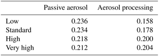
Table 1Parameters of the aerosol size distribution in the boundary layer prescribed in the initial and lateral boundary conditions.
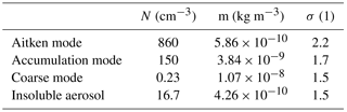
Table 2Parameters used for the representation of the different hydrometeor types (x: cloud, rain, ice, snow, and graupel). The size distributions of all hydrometeors are described as gamma distributions with a fixed curvature μx. The relation between particle mass Dx and particle diameter mx is described by ; the relation between Dx and the terminal fall velocity vx by .
Aerosol initial and boundary conditions are prescribed based on aerosol size distributions derived from aircraft observations (see Sect. 2.3). A profile of aerosol mass and number densities has been derived by combining data from a below cloud-base flight leg carried out in the morning and various cloud-free flight segments at higher altitude. In the boundary layer and free troposphere a vertically uniform mass mixing ratio and number concentration are used for each aerosol mode (Fig. S1b, c and Table 1). A linear transition between the two concentrations is assumed in a 500 m vertical slice centred at the mean boundary layer top (z = 1.15 km). A total of 10 % of the observed accumulation-mode aerosol is considered to be insoluble and to act as ice-nucleating particles in the model. No surface sources of aerosol have been included. Neglecting surface sources is not expected to have a large impact on the simulations because (i) the chosen aerosol profiles are based on observational data over the peninsula and therefore are representative of the environment in which the clouds form and (ii) the residence time of air in the model domain is only several hours (based on an average flow velocity of 7.5 m s−1 and a domain length of 225 km). According to the National Atmospheric Emissions Inventory data for 2014 (NAEI, 2014), the average PM2.5 (PM1) emission flux over the model domain is (). Assuming the emitted aerosol is evenly distributed over the boundary layer and with a mean flow velocity of 7.5 m s−1, the resulting change in aerosol mass mixing ratio is (). This corresponds to about 1 % (0.5 %) of the total aerosol mass or 5 % (2 %) of the accumulation-mode aerosol mass in the boundary conditions. In addition, the aerosol replenishment by advection from the boundary of the domain that maintains the initial profile is sufficient to avoid a very strong depletion by scavenging inside the domain (see Sect. 4). Therefore, we have ignored local aerosol emissions.
For the perturbed aerosol simulations, the aircraft-derived aerosol profiles are multiplied by factors of 10 and 0.1 at all altitudes, while conserving the mean diameter of each mode. These simulations are referred to as “high-aerosol” and “low-aerosol” runs, respectively. For additional tests on the thermodynamic limitations of the precipitation response, simulations with aerosol concentrations increased by a factor of 30 were conducted (“very high aerosol”). The simulation with the unperturbed aircraft-derived profile is named the “standard-aerosol” run.
2.2 CASIM microphysics and aerosol processing
Cloud microphysical processes and their interaction with the aerosol environment are represented by the newly developed CASIM module (Grosvenor et al., 2017; Hill et al., 2015; Shipway and Hill, 2012). The CASIM module is a double-moment, five hydrometeor classes microphysics scheme. The hydrometeor size distribution for each category is described by a gamma distribution, two moments of which (the mass and number mixing ratios), are prognostic variables. In addition, fixed densities, diameter–mass relations, and diameter–fall-speed relations are assumed for each hydrometeor category (Table 2). The simulated precipitation rate and reflectivity distributions are particularly sensitive to the assumed graupel density and diameter–fall-speed relation (not shown). We have chosen to use the diameter–fall-speed relation for medium-density graupel from Locatelli and Hobbs (1974) with a graupel density of 250 kg m−3, since this results in the closest agreement between modelled and observed reflectivity and surface precipitation rates (not shown). Represented transfer rates between the different hydrometeor categories and water vapour include droplet activation (Abdul-Razzak and Ghan, 2000; Abdul-Razzak et al., 1998), condensation (using saturation adjustment), primary ice formation from cloud droplets (DeMott et al., 2010), freezing of rain drops (Bigg, 1953), secondary ice formation from rime splintering in the Hallett–Mossop temperature zone, vapour deposition, evaporation, sublimation, collision–coalescence between all hydrometeor categories, and sedimentation of all hydrometeor categories except cloud droplets.
Aerosols are represented by three soluble modes and one insoluble mode that are described by a log-normal distribution with a prescribed width (Table 1). The aerosol mass mixing ratio and number mixing ratio are prognostic variables. The chemical and physical particle properties (density, solubility, etc.) are prescribed for each mode separately. The aerosol fields are initialised from a spatially homogeneous aerosol profile, which is also used for the lateral boundary conditions throughout the simulations. The aerosol fields are subject to advection.
For the aerosol–cloud interaction, two different modes are available within CASIM: (i) one-way coupling of aerosols and cloud properties (passive mode) and (ii) two-way interaction between aerosols and clouds (processing mode). In the passive mode, aerosol fields are considered in the droplet activation and primary ice nucleation, but the aerosol fields are not modified by cloud microphysical processes. We note that, while aerosols are not scavenged, this does not lead to an infinite supply of droplets. In the passive mode, the activation scheme will only activate additional droplets if the current population is lower than that expected by activation for the current grid-cell conditions. In the processing mode, aerosol fields are modified consistently with the cloud microphysical processes. The interstitial aerosols are depleted by nucleation scavenging (droplet activation and primary ice nucleation). Impaction scavenging is currently not represented. Previous work suggests that in-cloud scavenging is the dominant wet aerosol removal processes and that impaction scavenging is only important below cloud base (Flossmann et al., 1985; Yang et al., 2015). Therefore, omitting impaction scavenging should have no major implications for the present study. Droplet activation takes into account the different soluble aerosol modes according to Abdul-Razzak and Ghan (2000), while a small constant fraction of the insoluble aerosol mode is activated in water-supersaturated conditions. For the ice nucleation all insoluble aerosols, i.e. both interstitial and CCN (cloud condensation nuclei) activated insoluble aerosol, are used for the computation of ice crystal number concentrations to be consistent with the formulation in DeMott et al. (2010). Additional tracers for the soluble and insoluble aerosol mass as well as insoluble aerosol number in liquid and frozen hydrometeors are included. These tracers are subject to sedimentation fluxes of the respective hydrometeors and advection. During evaporation and sublimation aerosols are released into the interstitial aerosol modes according to their diagnosed effective radius and the effective radius of the interstitial aerosol modes. One soluble aerosol particle is released for each evaporating hydrometeor. Therefore, hydrometeor collision–coalescence results in fewer, but larger, interstitial aerosols if the hydrometeors subsequently evaporate. For insoluble aerosols, the activated number and mass are tracked. The number of insoluble aerosols released upon evaporation or sublimation of the hydrometeor is identical to the number of insoluble aerosol particles in the hydrometeor. Therefore, the number of insoluble aerosols is retained and is not impacted by collision–coalescence processes.
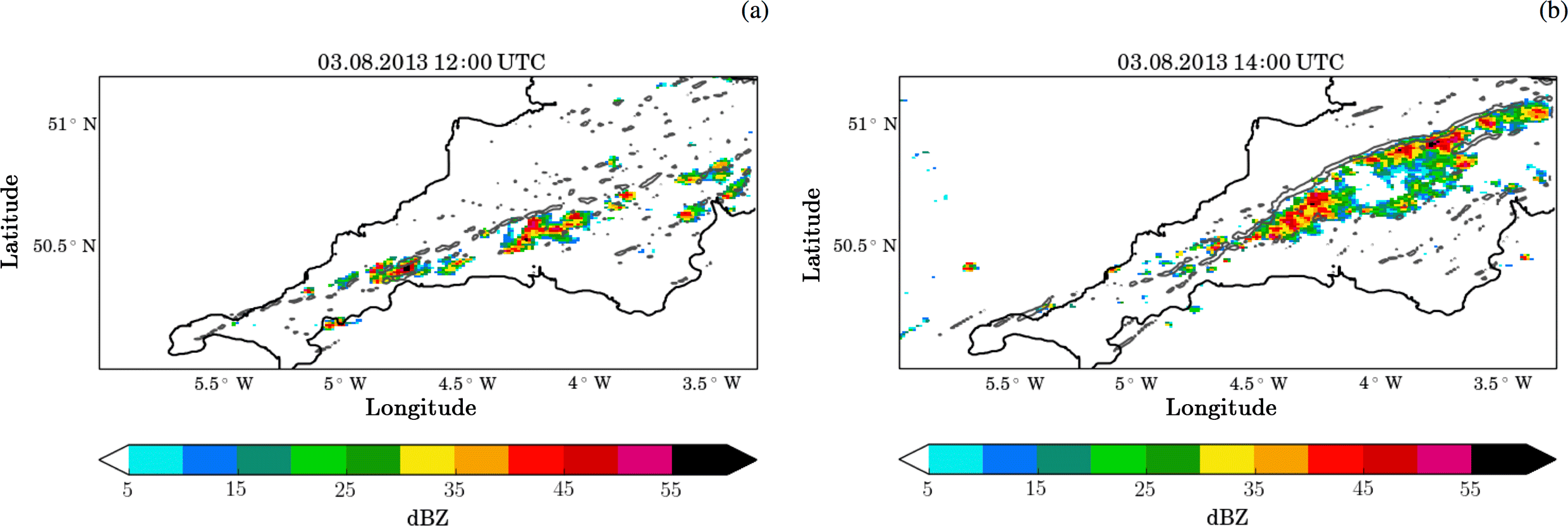
Figure 1Column maximum radar reflectivity (shading) over the COPE domain at (a) 12:00 UTC and (b) 14:00 UTC from the model simulation with passive aerosol and the standard-aerosol profile. The grey contour lines indicate convergence of at 250 m above ground.
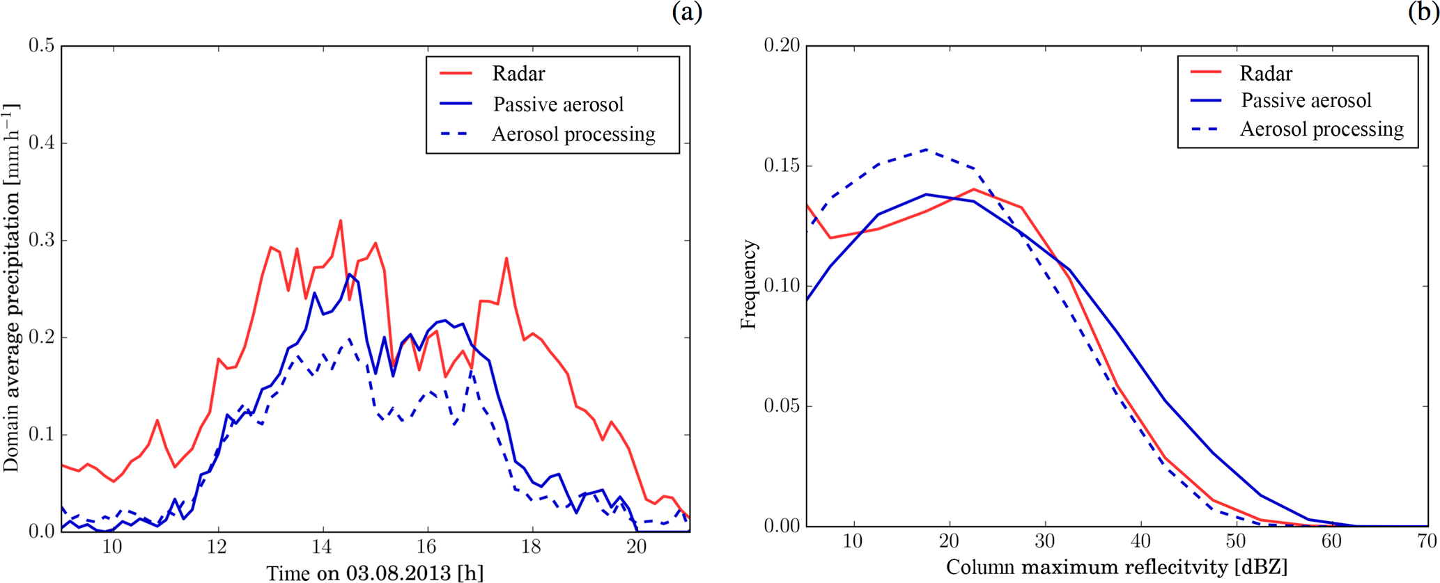
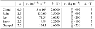
Figure 2Comparison of (a) the time series of domain-mean surface precipitation rate and (b) the normalised distribution of column maximum radar reflectivity from model simulations with the standard-aerosol profile (blue) and radar observations (red). The distribution includes only grid points with column maximum reflectivity larger than 0 dBZ. The solid line shows results from the simulation with passive aerosols and the dashed line from the simulation with aerosol processing. Simulated precipitation rates and radar reflectivity have been coarse-grained to the spatial resolution of the radar observations (1 km horizontal and 500 m vertical).
Simulations were conducted with passive and processing aerosol treatments. The impact on the model performance and the simulated hydrometeor and aerosol fields are discussed in Sects. 3 and 4, respectively.
2.3 Observational data from COPE
For the evaluation of the model simulations, we make use of the observational data gathered from various platforms during the COPE campaign. The details of the experiment design are outlined in Blyth et al. (2015). Leon et al. (2016) presented an overview of the campaign results. This study utilises radiosonde data and observations made with the Facility for Airborne Atmospheric Measurements (FAAM) BAe-146 research aircraft. Radiosondes were launched at roughly 2-hourly intervals from Davidstow (50.64∘ N, 4.61∘ W) between 08:00 and 15:00 UTC. These provide profiles of air temperature, dew-point temperature, and wind vectors.
The aerosol initial conditions were derived from data collected by the FAAM BAe-146 aircraft. Three instruments with overlapping size ranges were utilised: a scanning mobility particle sizer (SMPS) for measurements from 0.01 to 0.3 µm diameter with a 30 s scan time, a wing-mounted passive cavity aerosol spectrometer probe (PCASP) for measurements from 0.1 to 3 µm, and a wing-mounted cloud droplet probe (CDP) for measurements from 2 µm and above. The PCASP and CDP were calibrated using the methods of Rosenberg et al. (2012). The data were split into out-of-cloud straight-and-level legs spanning an integer number of SMPS scans. For each of these legs, a three-mode log-normal distribution was fitted to the data. No refractive index corrections were made to account for the potential different compositions of the aerosol. However, as we use just a single average profile for each of the boundary layer and the free troposphere, any refractive index correction is much smaller than the variability in the measurements.
Cloud droplet number was also provided by the CDP. The sensitive sample area of this instrument was calibrated using a droplet generator and found to be approximately twice the nominal sample area in the manufacturer's specification. Vertical wind measurements were provided by a five-port turbulence probe on the aircraft nose combined with Pitot tube airspeed measurements and GPS–inertial-navigation-unit aircraft altitude information (Petersen and Renfrew, 2009).
In addition to the campaign-specific data, we use a 3-D radar composite provided by the Met Office (Scovell and al Sakka, 2016). The composite data used here have a horizontal resolution of 1 km, a vertical resolution of 500 m over the study area, and a temporal resolution of 10 min. In addition, we use the Radarnet IV rainfall retrieval (Harrison et al., 2009; MetOffice, 2003), which is also based on the operational radar network. The horizontal resolution is 1 km and the temporal resolution 5 min.
3.1 Radar reflectivity and surface precipitation
The model simulations capture the general evolution of the cloud band and the major structural features as described in the introduction (Fig. 1, Supplement Figs. S3 and S4): the first larger clouds (maximum dimension of areas with column maximum reflectivity larger than 25 dBZ exceeding 10 km) appear after 11:00 UTC and are organised along a line roughly along the axis of the peninsula. In the subsequent hours, clouds cluster along the convergence line with cells remaining more isolated and smaller over the western half of the peninsula and larger clusters developing further east. While the majority of clouds develop along the convergence lines, some more isolated clouds develop in other parts of the domain. A double line feature appears in some model simulations, but is not as well defined as in the observational radar data. In agreement with observations, the modelled cloud line slowly assumes a more northeasterly orientation throughout the day. The line of convective clouds starts to dissipate at around 17:00 UTC, i.e. slightly earlier than in the observations.
The domain-average surface precipitation rates from the operational radar network (Harrison et al., 2009; MetOffice, 2003) and the model simulations with the standard-aerosol profile are compared in Fig. 2a. The radar data show some precipitation from isolated convective cells before 11:00 UTC. The simulated domain-average precipitation during this initial time period is much lower, but the average cell precipitation rate is comparable (excluding grid points with no precipitation, Fig. S5a). The simulated cells are less numerous and remain smaller (Fig. S5c, d). The lack of development of larger cells is consistent with the previously described tendency of high-resolution models to produce too many too-small cells (Hanley et al., 2015; Stein et al., 2015). In contrast to the weakly forced convection in the morning, the organisation into larger cells later in the simulation is supported by the establishment of sea-breeze convergence lines (Fig. S5b). Domain-mean precipitation rapidly increases between 11:00 and 13:00 UTC in the radar observations and between 11:00 and 14:00 UTC in the simulations. During the afternoon, both data sets show consistently high surface precipitation rates until about 17:00 UTC (model) and 18:00 UTC (observations). The cessation of precipitation is linked to the dissolution of the convergence lines (Fig. S5b). While the model captures the main evolution of the precipitation linked with the convergence lines, the peak domain-mean precipitation rate occurs about an hour later than in the radar data. The model underestimates the domain-mean surface precipitation relative to the radar-derived precipitation irrespective of the chosen aerosol treatment. In contrast to domain-average precipitation, cell average precipitation is overestimated (Fig. S6a). This indicates that too few instances with surface precipitation are simulated. In particular, instances of weak precipitation (), both over all data points and over raining data points only, are underestimated (Fig. S6a, b). High precipitation rates are overestimated by a factor of 2 relative to the radar-derived estimate (Fig. S6a, b).
Quantitative estimates of precipitation rates from radar reflectivity can exhibit biases due to assumptions of hydrometeor properties and the representation of sub-cloud evaporation in the algorithm used to derive rain rate from radar observations. In addition, beam blocking can significantly affect low-level radar reflectivity. We therefore compare diagnosed radar reflectivity from the simulations with a 3-D radar composite (Fig. 2b and Fig. S6c, d). The distribution of column maximum reflectivity, also known as composite reflectivity, for cloudy grid points is shown in Fig. 2b. The observed and modelled distributions are in good agreement: the most frequent column maximum radar reflectivity is about 5 dBZ too low in both simulations and the peak reflectivity is overestimated by about 5 dBZ in the passive-aerosol simulation. The occurrence of low reflectivity values (<10 dBZ for passive aerosol, <5 dBZ for aerosol processing) is underestimated (Fig. 2b). The frequency distribution computed over all grid points, i.e. taking into account the fraction of the domain covered by clouds, indicates an underestimation of column maximum reflectivity for values smaller than 40 dBZ in the simulation with passive aerosols (Fig. S6d). In contrast, all reflectivity values occur with larger frequency in the observations than for the simulations with aerosol processing. This again indicates too few occurrences of cloudy grid points in the model (Fig. S6d).

Figure 3Cloud base cloud droplet number density as a function of vertical velocities from aircraft data (red symbols) and model data (grey shading). Panel (a) shows the simulation with passive aerosols and panel (b) the simulation with aerosol processing. The simulations in both panels use the standard-aerosol profile. Aircraft observations include data collected during low-level flight legs close to cloud base (, 12:00 to 12:50 UTC). CDP measurements are used for the cloud droplet number concentrations and Airborne Integrated Meteorological Measurement System (AIMMS)-20 measurements for the vertical velocity. Cloud base cloud droplet number density and vertical velocity in the model is retrieved from the lowest model level with a cloud droplet mass larger than 1 mg kg−1 from the entire domain between 12:00 and 13:00 UTC.
Surface precipitation is more closely linked to cloud base reflectivity than to column maximum reflectivity. The distribution of in-cloud low-level radar reflectivity (at 750 m) from the passive-aerosol simulation indicates an underestimation in the frequency of reflectivity values between 20 and 30 dBZ (Fig. S6c). Above 35 dBZ the modelled frequency of occurrences is overestimated in the simulation with passive aerosols and almost identical to the observed distribution in the simulation with aerosol processing. In the simulation with aerosol processing, the reflectivity in this range is also underestimated, but the occurrence of reflectivity smaller than 10 dBZ is overestimated.
The overall agreement between the observed and the modelled radar reflectivity distributions is better than that seen between the radar-derived rain rate and model rain rate. However, both variables indicate an underestimation of the occurrence of cloudy points (in space and time). The better agreement with radar reflectivity may suggest potential problems with the radar-derived surface precipitation for medium to low precipitation rates, e.g. due to the missing representation of sub-cloud evaporation in the retrieval of surface rain rates from radar data (Li and Srivastava, 2001). Another possibility is issues with the diagnosed reflectivity from the model simulations, which does not account for extinction, non-spherical drops, or contributions from Mie scattering (Oguchi, 1983).
The 3-D radar composite also provides information on the cloud structure. Here we compare the largest altitude at which the radar reflectivity exceeds 18 dBZ in each column. The 18 dBZ contour is often used in radar data sets to determine the “echo top” (Lakshmanan et al., 2013; Scovell and al Sakka, 2016). The mean height of the 18 dBZ contour increases from about 2 km in the morning to 3 km in the afternoon in the observations and the model simulations (Fig. S7a). This indicates a general deepening of convective cells in correspondence to larger convergence as the sea-breeze lines establish (Fig. S5b). The modelled mean height of the 18 dBZ contour agrees within 200–500 m with the one derived from the 3-D radar composites (Fig. S7a). The maximum height of the 18 dBZ contour in the observations only shows a small increase from about 5 km to about 5.5–6 km between 10:00 and 13:00 UTC, while in the model the maximum height increases from 3.5 to 5–5.5 km (Fig. S7b). The larger maximum heights in the radar observations are mainly due to higher-level ice clouds that are not present in the model simulations. The modelled and radar-derived domain-average heights of contours between 5 and 25 dBZ differ by a maximum of 500 m (not shown). The model tends to underestimate (overestimate) the mean altitudes for lower (higher) reflectivity values. Given the vertical resolution of the radar data set (500 m) and the model-level spacing (200 m at 5 km), this is a reasonable agreement.
3.2 Aircraft observations of hydrometeor number concentrations
The fraction of aerosol activated to cloud droplets is important for the aerosol effect on clouds. We therefore compare the cloud base cloud droplet number concentration measured by the CDP on-board the BAe-146 with the modelled cloud base droplet number concentration (Fig. 3). The aircraft data are taken from several flight legs close to cloud base (within 500 m) sampling multiple cells along the convergence lines between 12:00 and 12:50 UTC (red dots). In the model all clouds in the domain are sampled within the same time period (grey shading). Cloud base in the model is defined as the lowest vertical level in each column with a cloud droplet mass larger than 1 mg kg−1. CDNC at cloud base generally increases with the vertical velocity in the simulations and the observations, as expected. Sensitivity experiments with the aerosol size distribution used in the model suggest that a multi-mode representation of aerosols is required to match the observed relation over the range of cloud base updraft velocities (up to 7 m s−1) (not shown). CDNC values in the observations reach about 375 cm−3, which is most closely matched by the simulation with aerosol processing (Fig. 3b). The simulation assuming passive aerosols over-predicts maximum CDNC values by about 30 % (Fig. 3a).
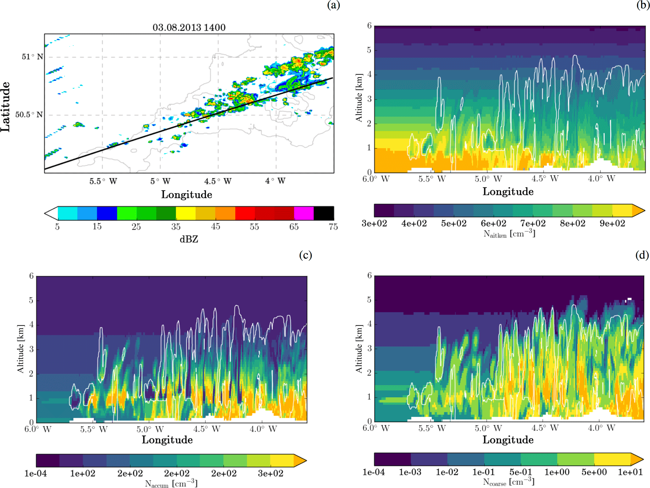
Figure 4Aerosol fields from the simulation with aerosol processing at 14:00 UTC. (a) The colour shading shows the column maximum reflectivity and the black line indicates the location of the cross sections plotted in the other panels: (b) number density of Aitken-mode aerosol, (c) accumulation-mode aerosol, and (d) coarse-mode aerosol. The white contour lines in panels (b, c, d) indicate areas with hydrometeor mixing ratios larger than 1 mg kg−1.
Combining aircraft data from cloud penetrations at various altitudes throughout the day provides some information of the CDNC variation with height above cloud base. The observational data in general suggest a decrease in the maximum observed CDNC with altitude above cloud base (Taylor et al., 2016b). In the simulation with passive aerosol, mean CDNC decreases slowly with height. However, CDNC values remain comparable to the cloud base values at all levels within the clouds (Fig. S8a). In the simulation with aerosol processing, CDNC decreases more rapidly above cloud base and the spread is significantly larger than for the passive-aerosol simulations (Fig. S8b), i.e. a behaviour more compatible with observational data. However, a direct comparison to the model results is not possible, since the location of the aircraft observations relative to updraft cores is not known.
3.3 Radiosonde data
The overall structure of the thermodynamic profiles in the model is similar to the 2-hourly radiosonde data at Davidstow (Fig. S9). The radiosonde data were compared to the thermodynamic profile at the grid column closest to the release location of the radiosonde. The temperature agrees within ±1 K and the dew-point temperature within ±5 K (±10 K) below (above) a stable layer located between 5 and 6 km altitude. As discussed later, the stable layer at 5–6 km is an important feature of the thermodynamic profile for the aerosol-induced changes. This stable layer is located at the same altitude in the simulations and the observations (Fig. S9). Other parameters, such as the height of the 0∘C level and the lifting condensation level, are similar in the model and the observational data throughout the day with maximum deviations of 100 and 250 m, respectively (Fig. S10).
The model simulations using the standard-aerosol profiles compare favourably with radar and aircraft observations (air and dew-point temperature profiles differences smaller than ±1 and ±5 K, respectively; 0∘C level, lifting condensation level, and height of the 18 dBZ contour within ±250 m; cloud base CDNC differences smaller than 30 %; domain-average precipitation and precipitation rates larger than 4 mm h−1 within a factor of 2; radar reflectivity within ±5 dBZ for reflectivity larger than 5 dBZ). This suggests that the model is adequately representing the processes important for this case, providing confidence that changes predicted by aerosol perturbation experiments will be physically meaningful.
Cloud microphysical processes can alter the aerosol fields by changing the aerosol size distribution, the aerosol chemistry, or by redistributing or removing aerosols. While these feedbacks are often not represented in numerical weather prediction models, they can be represented with the CASIM module, except for changes to the aerosol chemistry. In this section we discuss the changes in aerosol and hydrometeor number density resulting from the representation of the two-way coupling between aerosol and cloud microphysics. We only discuss simulations with the standard-aerosol profile.
In the passive-aerosol run, the aerosol fields are only subject to advection and are not modified by cloud microphysical processes. Therefore, only minor changes in the aerosol concentrations relative to the prescribed profile occur (Fig. S11: compare profile at upstream, i.e. western, boundary with rest of domain). Hovmöller diagrams of aerosol loading (vertically integrated and latitudinally averaged aerosol concentrations) confirm this picture for the entire duration of the simulation (Fig. S12a, c, e). Small decreases and increases occur in regions of divergent and convergent flow, which are likely related to gravity waves excited by the sea-land contrast (5.5∘ W) and orography (4.5 and 4.0∘ W).
In the aerosol-processing run, aerosol fields are modified according to microphysical processes. The additional tendency terms for the aerosol fields include (i) depletion of interstitial aerosol number and mass during cloud droplet activation and ice nucleation and (ii) increases in interstitial aerosol number and mass during evaporation and sublimation. Collision–coalescence reduces the number of aerosol particles released during evaporation compared to the number originally activated. Hence, for example, aerosol activated from the Aitken-mode population may be released back into the interstitial aerosol population in the accumulation mode. Changes in the aerosol field relative to the passive-aerosol simulation or to a good approximation of the upstream boundary can be directly attributed to either of these processes. Cross sections of the aerosol concentrations along the convective line are shown in Fig. 4. The Aitken-mode aerosol is depleted within cloud, below cloud, in areas of evaporated clouds (e.g. around 5.25∘ W), and in the outflow at higher levels. The reduction occurs in regions where activation is expected and in downstream areas. The accumulation-mode aerosol is also reduced inside clouds where activation is expected. The reduction in aerosol in these regions is due to nucleation scavenging because this is the only process that can consume interstitial aerosol in the model. Below cloud base and in areas of evaporated clouds, accumulation-mode aerosols are enhanced compared to the upstream profile. Similar increases in the number concentration occur at the lateral boundaries of clouds. These are regions where evaporation of hydrometeors takes place. Therefore, increases in accumulation-mode number concentration can be explained by evaporation of larger cloud droplets or rain drops. The coarse aerosol mode behaves very similarly to the accumulation-mode aerosol, but increases compared to upstream conditions are more widespread and have a larger amplitude.
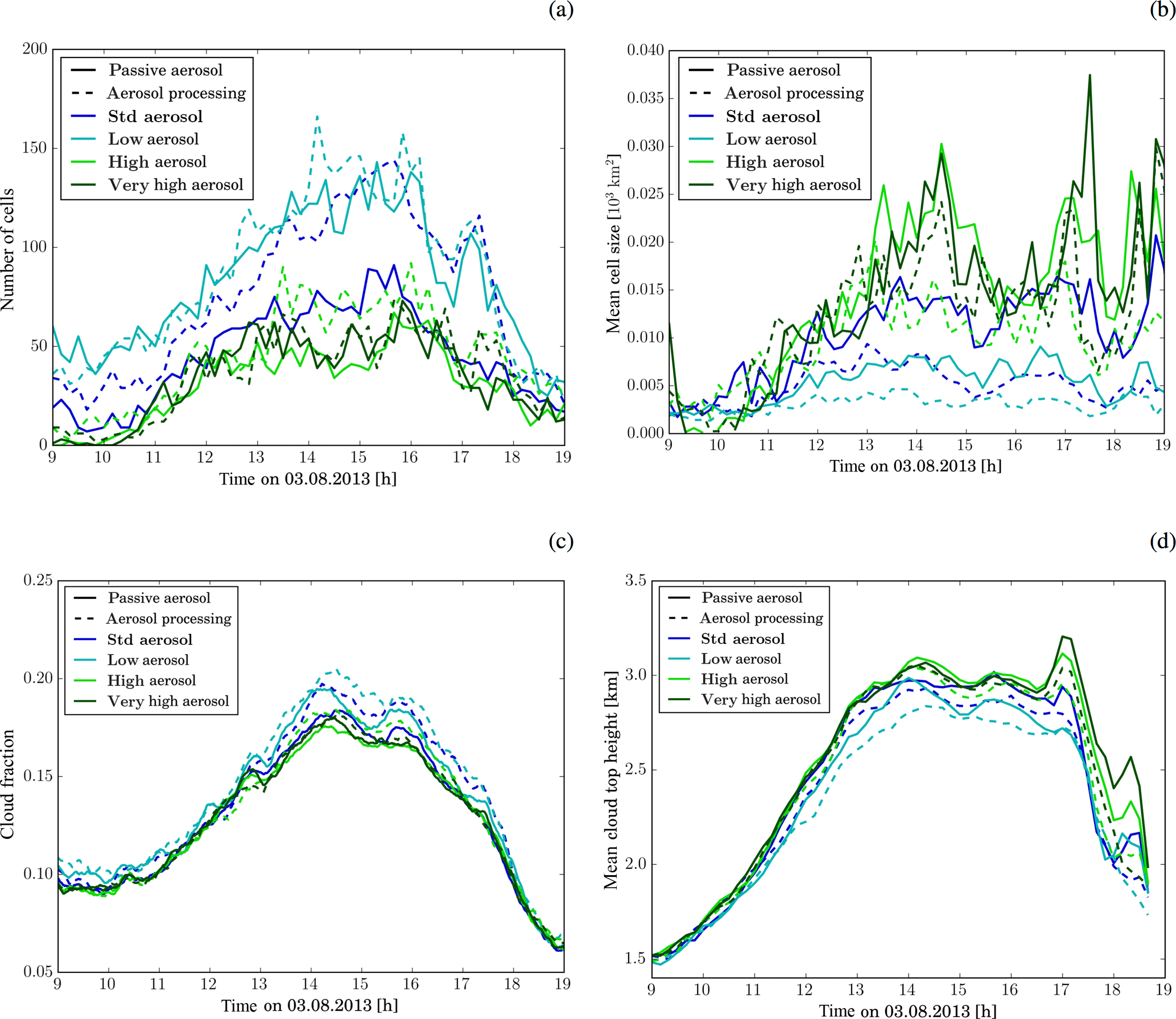
Figure 5Time evolution of (a) number of cells, (b) average cell size, (c) cloud fraction, and (d) domain-average cloud top height. Cloudy areas are defined as having a water path larger than 1 g m−2. Cells are defined as coherent areas with a column maximum radar reflectivity larger than 25 dBZ. Different line colours indicate the different aerosol initial conditions. Solid lines correspond to simulations with passive aerosols and dashed lines to simulations with aerosol processing.
The impact of aerosol processing seen in the cross section is representative of the modifications that the model imparts to aerosol fields during the entire simulation (Hovmöller diagrams of aerosol loading: Fig. S12b, d, f). Aitken-mode aerosols are depleted at the outflow (eastern) boundary relative to the values at the inflow (western) boundary, while accumulation-mode and coarse-mode aerosol increases. In the time interval between 09:00 and 20:00 UTC, the Aitken-mode number concentration reduces on average by 7 %, the accumulation-mode number concentration increases by 15 %, and the coarse-mode number concentration increases by a factor of 10 across the study area (4.61 to 3.5∘ W). These estimates discount any clouds present at the downstream boundaries and take only cloud-free areas into account. The predicted changes in the coarse-mode aerosol concentrations are large enough that they eventually could be identified in future aircraft campaigns by flying long north–south-oriented runs up- and downstream of the convective line. Such observations would provide valuable information for the evaluation of the model representation of aerosol–cloud interactions.
Aerosol processing reduces the total number of aerosol available at cloud base due to the modification of the aerosol size distribution by collision–coalescence (Fig. 4). This impacts the mean (maximum) cloud base droplet number concentration, which is reduced by 50 % (10 %) compared to the simulations with passive aerosols. The reduction of aerosol number concentration at cloud base is particularly relevant for clouds developing along the eastern part of the convergence line, where aerosol concentrations in the boundary layer have been modified by previous clouds (Fig. 4). In addition to the impact on the overall number concentration, aerosol processing changes the relative contributions from each aerosol mode (Fig. 4). Therefore, aerosol processing impacts the relation between CDNC and vertical velocity at cloud base as discussed in Sect. 3 (Fig. 3). Further differences occur in the vertical distribution of CDNC within the cloud (Fig. S8). With aerosol processing, a larger variability of CDNC values occurs and CDNC decreases more strongly towards cloud top. Activation in the model occurs where CCN concentrations predicted by the Abdul-Razzak et al. (1998) parameterisation (based on vertical velocity and aerosol concentration) exceed the CDNC present in the grid box. The maximum CDNC in the passive-aerosol simulation is almost constant with altitude. We interpret this as a result of activation at higher altitudes enabled by the high interstitial aerosol concentrations in the cloud. In contrast, maximum CDNC values decrease with altitude in the aerosol-processing run. In this simulation, nucleation scavenging is taken into account and the therefore reduced interstitial aerosol concentrations impede any activation above cloud base. This argumentation assumes no major differences in the vertical velocity, which is justified by the rather small differences of in-cloud kinetic energy discussed later (Sect. 6.2).
Cloud properties and precipitation are influenced by the aerosol available during cloud formation. To investigate the sensitivity of the studied cloud field to different aerosol concentrations, we conducted simulations with enhanced and reduced aerosol concentrations in the initial and lateral boundary conditions (see Sect. 2.1). The impact of these perturbations on the cloud field and precipitation is described in this section, while the physical mechanisms responsible for the changes are discussed in Sect. 6.
5.1 Cloud field structure and cloud geometry
Cloud fields from simulations with higher aerosol concentrations are more organised with larger, less widespread, and more densely packed cells (qualitative: Fig. S13). The changes to the cloud field structure can be quantified by comparing the number of cells and the mean cell size (Fig. 5a, b). A cell is defined as a coherent area with a column maximum radar reflectivity larger than 25 dBZ. The number of cells decreases and the mean cell size increases with larger aerosol concentrations throughout the simulation. The cell number changes in all development stages of the convective line, while the change in cell size is particularly evident in the afternoon (after about 13:00 UTC). Aerosol-induced changes in cell number and size are smaller for aerosol concentrations enhanced above the standard-aerosol profile compared to reduced aerosol concentrations. The transition to a more structured cloud field in the high-aerosol environment is accompanied by a small reduction in cloud fraction (Fig. 5c). The cloud fraction is defined as the proportion of the domain covered by clouds with a condensed water path larger than 1 g m−2. Changes in cell number and size change in opposition such that aerosol-induced changes in cloud fraction are very small and occur mainly between 13:00 and 16:00 UTC.
The average cloud top height rises in high-aerosol environments (Fig. 5d). Cloud top height is defined as the altitude of the highest grid box with a condensate content larger than 1 mg kg−1 in each column. Differences in mean cloud top height are small in the development phase of the convective line but amount to about 100–200 m in the afternoon. The increase in mean cloud top height is due to a reduced occurrence frequency of cloud tops between 3 and 4 km and an increased occurrence frequency of cloud tops above 4.5 km (Fig. S14a). Cloud base height variations between simulations with different aerosol profiles are much smaller (mean height ±50 m, Fig. S14b). Aerosol-induced changes in cloud top height are larger in the aerosol processing than the passive-aerosol simulations. The maximum cloud top height is restricted by a stable layer extending from about 5–6 km, which is evident in the thermodynamic profiles from radiosondes and model simulations (Fig. S9). In the simulations with passive aerosols, the cloud tops reach the stable layer under standard aerosol concentrations, while they only reach this altitude under enhanced aerosol concentrations in simulations with aerosol processing. Cloud deepening from the standard to the high-aerosol scenario is not limited by the thermodynamic profile in the aerosol-processing case, while it is in simulations with passive aerosols. For the simulations with passive aerosol, a similar asymmetry in the response to increases and decreases in the aerosol concentration is also evident in other variables (Sects. 5.2 and 6). We hypothesise that this asymmetry is controlled by thermodynamic constraints on the cloud top height. This hypothesis is further discussed in Sect. 6.
5.2 Surface precipitation
The overall precipitation response to changes in the aerosol profile can be divided into two different periods (Fig. 6b). An early period (09:00–12:00 UTC) during which the precipitation decreases with increasing aerosols and a later period (12:00–20:00 UTC) during which precipitation increases with increasing aerosols in most cases. For the high and very high-aerosol scenario, accumulated precipitation decreases in the later period relative to the simulation with the standard-aerosol profile. The continuous decrease in precipitation with aerosol concentration in the first period agrees with parcel model results indicating a less efficient collision–coalescence in the presence of more CDNC (Feingold et al., 2013; Twomey, 1966). However, contrary to the precipitation suppression idea, the accumulated precipitation increases with enhanced aerosol concentrations in the afternoon. The underlying physical processes are discussed in Sect. 6. The transition from precipitation suppression to enhancement coincides roughly with the transition from isolated and unorganised convective clouds to on average larger and deeper cloud clusters forming along the converging sea-breeze fronts (Figs. S3, S4).
The accumulated surface precipitation depends on the chosen aerosol representation (Fig. 6a). In simulations with aerosol processing, the accumulated precipitation is about 20 % smaller than in simulations with passive aerosols. Including aerosol processing in the simulations results in a larger aerosol-induced change in accumulated precipitation with a maximum change of 14 % (standard- to high-aerosol scenario, aerosol processing) compared to 4 % (low- to standard-aerosol scenario, passive aerosol). The transition from precipitation suppression to enhancement occurs with aerosol processing and passive aerosol.

Figure 6(a) Time evolution of accumulated precipitation since 09:00 UTC. (b) Change in accumulated precipitation relative to simulations with the standard-aerosol scenario. Different line colours indicate the different aerosol initial conditions. Solid lines correspond to simulations with passive aerosols and dashed lines to simulations with aerosol processing.
The precipitation rate distribution is also influenced by the aerosol concentrations (Fig. S15). In the passive-aerosol simulations, medium rain rates (∼ 1–20 mm h−1) are more frequent and small rain rates less frequent with increasing aerosol concentrations. High precipitation rates () are less frequent both in the high and low scenario than in the standard-aerosol case. If aerosol processing is included, then changes in low and medium rain rates are much smaller and the probability of high rain rates () increases continuously with the aerosol concentration.
5.3 Condensed water content
Under enhanced-aerosol conditions, precipitation formation is thought to be suppressed due to a less efficient conversion of condensed water to precipitation-sized hydrometeors. Consistent with this idea, the domain-integrated condensed water path increases with the aerosol concentration in the time period of main convective activity, i.e. between 12:00 and 20:00 UTC (Fig. S16a). This increase is larger and extends to the entire simulated time period if only hydrometeors with small sedimentation velocities (cloud droplets, ice, and snow) are taken into account (Fig. S16b).
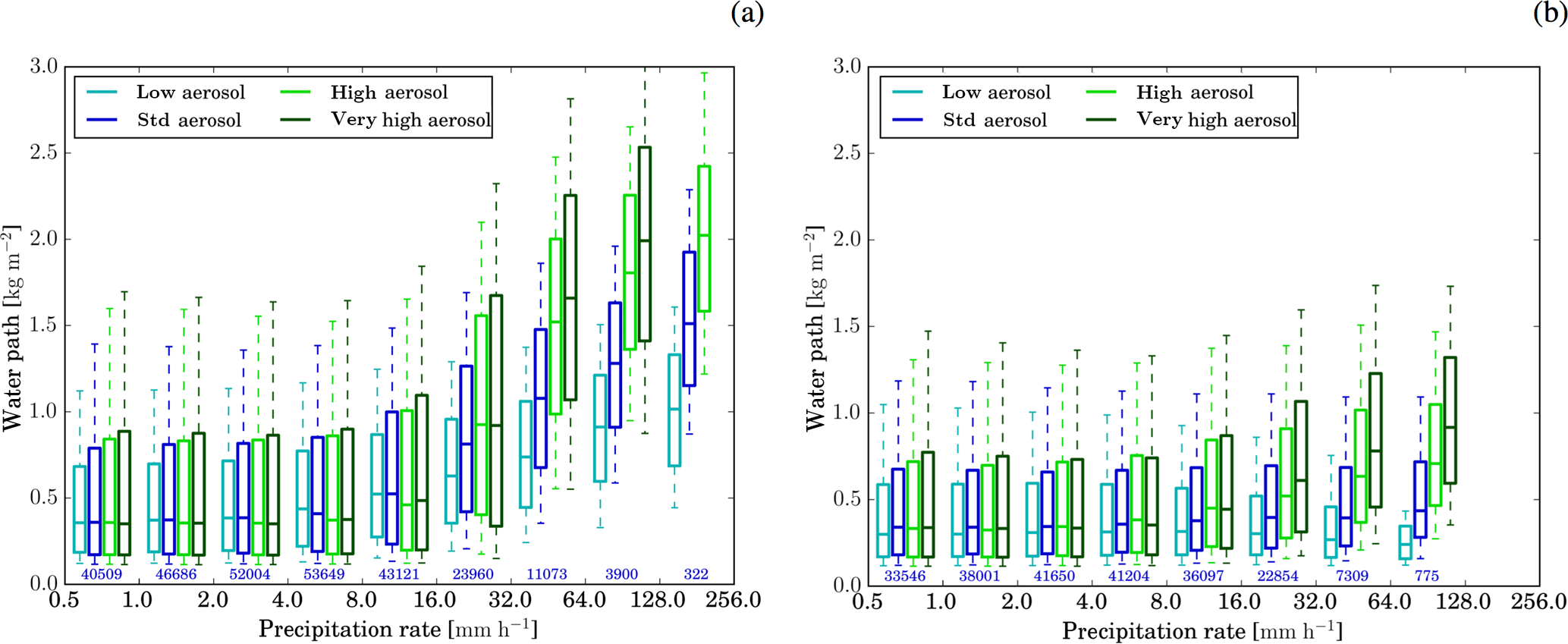
Figure 7The box and whisker plots show the distribution of the condensed water path (cloud and ice categories) in columns with certain precipitation rates for simulations with (a) passive aerosol and (b) aerosol processing. Different colours correspond to the different aerosol profiles. Values are only shown for precipitation bins with more than 100 data points. The median water path is shown by the horizontal line in the box. The boxes cover the interquartile range (25th to 75th percentile) and whiskers represent the 10th and 90th percentile, respectively.
Parcel model considerations suggest that a higher condensed water content is required to obtain the same precipitation rate for higher cloud droplet number concentrations. To investigate whether this also holds for the relation of condensate loading and precipitation in a more complex model, the distribution of condensed water path (in the ice and cloud droplet categories) in columns with a specific precipitation rate is displayed in Fig. 7. While there is no clear trend for precipitation rates up to 16 mm h−1, the median condensed water path increases strongly with aerosol concentrations for larger precipitation rates. For higher percentiles (75th and 90th percentile) an increasing condensed water path is also evident for small precipitation rates. A trend to a larger median condensed water path occurs also for low precipitation rates if only the first part of the simulation until 12:00 UTC is considered (Fig. S17c, d). In contrast, the distribution of condensed water paths for small precipitation rates does not depend on the aerosol scenario in the afternoon (Fig. S17e, f). The same trends occur in the simulations with aerosol processing and with passive aerosol, but the condensed water path dependency of surface precipitation is less pronounced in the aerosol-processing simulations. The behaviour of the total condensed water path (including all hydrometeor categories) is very similar to changes in the condensed water path including the cloud and ice category only (Fig. S17a, b).
6.1 Decomposition of precipitation response into changes in condensate generation and loss
Changes in precipitation can be contextualised and interpreted by investigating the condensate budget of the considered clouds (Altaratz et al., 2014; Barstad et al., 2007; Khain and Lynn, 2009). The change in precipitation at the surface ΔP is thereby considered as the result of changes in condensate gain ΔG (condensation and deposition of water vapour) and condensate loss ΔL (evaporation and sublimation). If changes in condensate gain are larger than changes in the loss terms, then surface precipitation increases and vice-versa. Furthermore, the ratio between ΔG and ΔL combined with the precipitation efficiency (PE) of the control simulation indicates whether changes in the condensate gain, i.e. changes in uplift, are driving surface precipitation responses or whether changes in precipitation efficiency, i.e. more or less efficient conversion of condensate to precipitation, are involved as well (see Appendix A). The analysis of the condensate budget provides insight into the influences of cloud microphysics, cloud dynamics, and the cloud environment on precipitation formation, because the condensate budget is intrinsically linked to latent heating, condensate distribution within the cloud, and different timescales of cloud microphysics and dynamics (Miltenberger et al., 2015; Stevens and Seifert, 2008).
The condensate budget approach requires (i) reasonable mass conservation properties of the underlying numerical model, (ii) no change in storage of condensate in the considered domain, and (iii) no change in advection of condensate out of the considered domain. The first requirement is ensured in our simulation by using the Aranami et al. (2014) and Aranami et al. (2015) approach to enforce moisture conservation in the regional model domain. Very little condensate is present in the domain at the start and end of the analysis period (09:00–20:00 UTC, Fig. S16a). Therefore, the second requirement is fulfilled to a very good approximation. The domain used in our simulation does not cover the entire length of the convergence lines and therefore condensate is advected out of the domain. To investigate the impact of the advection on the validity of the condensate budget analysis (requirement iii), we diagnose the advected condensate amount at the domain edge from meteorological fields at 10 min resolution. Figure 8a shows that the inclusion of the advective terms has a small impact on the changes in gain and loss terms (compare open and filled symbols). This suggests that changes in advective terms are small compared to changes in other terms of the condensate budget for our simulations. Advective terms will therefore be ignored for the rest of the analysis.
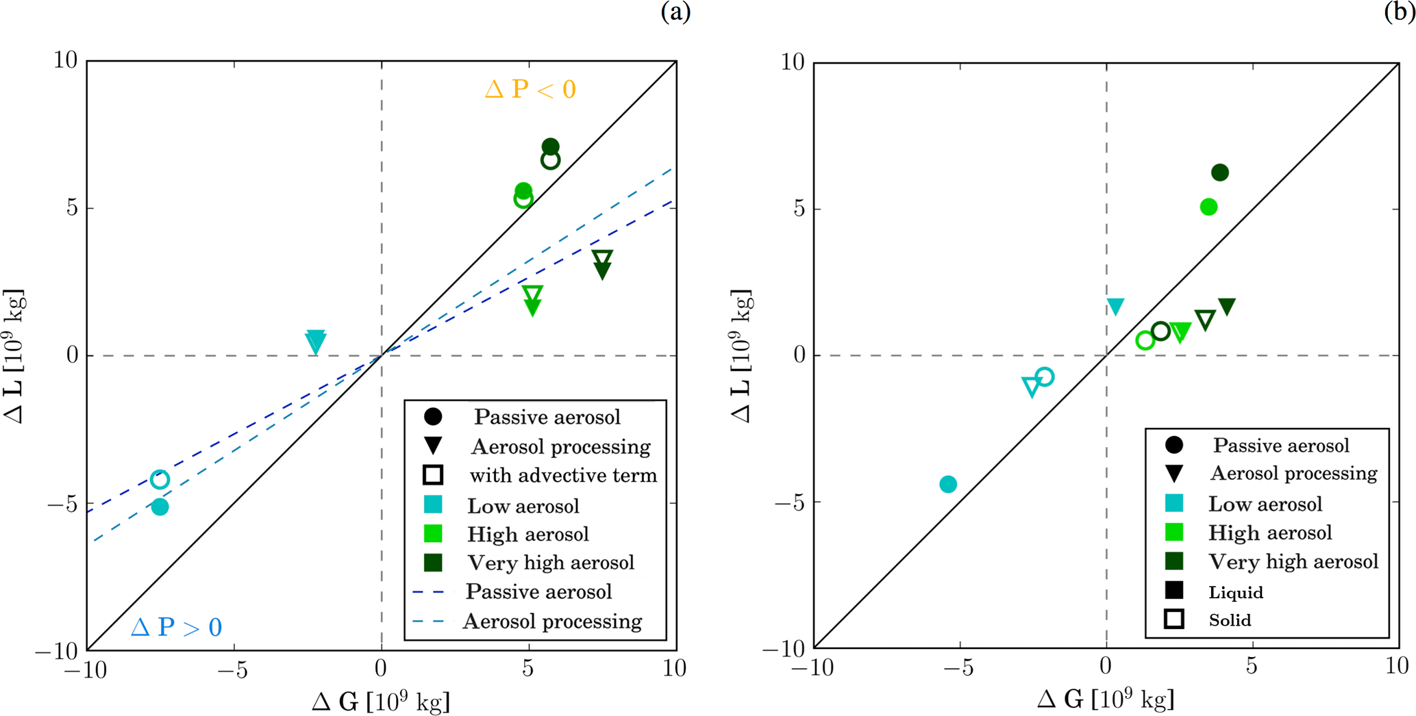
Figure 8(a) Scatterplot of change in condensate gain ΔG and loss ΔL relative to the simulation with the standard-aerosol profile. Points falling above the one-to-one line (solid black line) portray a decrease in surface precipitation, while points below it portray a surface precipitation increase. For points in the area between the solid black line and the dashed lines (dark blue: passive aerosol, light blue: aerosol processing) the change in condensate generation dominates over the change in PE (Appendix A). The impact of advection of condensed water out of the domain is illustrated by the open symbols. For these points the advective flux is discounted as loss. (b) Same as (a), but separating contribution of condensation and evaporation (filled symbols) from contribution of deposition and sublimation (open symbols).
The condensate budget terms are calculated by integrating condensation, evaporation, deposition, and sublimation rates over the model domain and the time period of convective activity, i.e. between 09:00 and 20:00 UTC. Changes in the condensate gain ΔG and loss ΔL relative to simulations with the standard-aerosol profiles are shown in Fig. 8a. In this plot all points above the one-to-one line correspond to simulations for which the condensate gain changes less than the condensate loss. Surface precipitation in the corresponding simulations is smaller than in the reference case, i.e. the standard-aerosol scenario. Points below the one-to-one line portray simulations with enhanced precipitation. The concept of this plot is discussed in more detail in the appendix and Fig. A1. The condensate gain increases with the aerosol concentrations for all simulations. However, the absolute value of ΔG decreases towards high-aerosol scenarios for the passive-aerosol simulations. In the highest-aerosol scenarios, cloud tops are located close to an upper-level stable layer as discussed in Sect. 5.1, which imposes a limit on further cloud deepening and the condensate gain. For simulations with aerosol processing, the absolute value of ΔG is smaller (larger) for the low (very high) aerosol scenario compared to the simulation with passive aerosol. Cloud tops in the aerosol-processing simulations are on average lower for a given aerosol scenario and therefore cloud deepening is not yet limited by the upper-level stable layer.
Table 3Precipitation efficiency (PE) of the different simulations. PE is defined as the ratio of domain-integrated precipitation to domain-integrated condensate gain.
The condensate loss also becomes larger with increasing aerosol concentrations. However, ΔL does not simply scale with ΔG, suggesting that changes in precipitation efficiency are important for the precipitation response as well. PE is defined here as the ratio of domain-integrated time-accumulated surface precipitation to the condensate gain. PE quantifies the efficiency of cloud microphysical processes in converting condensate to surface precipitation. The precipitation efficiency for the different simulations is listed in Table 3. In the simulations with passive aerosol, PE shows little change from the low to the standard aerosol number concentrations but decreases by about 2 % up to the very high-aerosol scenario. In contrast, in the simulations with aerosol processing, PE increases from the low to the high aerosol number concentration by about 4 %. For a further increase in the aerosol number concentration, PE increases more slowly. Cloud base precipitation efficiency, i.e. discounting sub-cloud evaporation of rain, is overall about 10 % larger but behaves in a similar way (not shown). These tendencies in PE may be related to changes in the graupel production rate. While the graupel mass mixing ratio increases with aerosol number concentrations in the aerosol-processing simulations, it decreases in the passive-aerosol simulations (Fig. S19b, d, f). Since graupel production rates depend strongly on the number and mean size of cloud droplets, it can be speculated that this difference between the aerosol-processing and passive-aerosol simulations is due to the different vertical variations in cloud droplet number density (see Sect. 4). The lower cloud tops in the aerosol-processing simulations may also play a role in the lower graupel production rate.
Table 4Change in surface precipitation expected from the simulated change in PE (left column) and the change in condensate generation (middle column). The last column gives the total relative change in precipitation, as predicted by the simulations. All changes are relative to the simulation with the standard-aerosol profile.
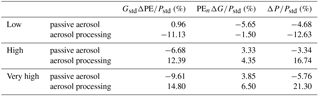
To investigate the relative importance of ΔG and ΔPE for the surface precipitation, the precipitation response is decomposed into the relative contributions according to Eq. (A2) (Table 4). The decomposition is graphically represented in Fig. 8a by the blue dashed lines. For simulations outside the area between the one-to-one line and the blue dashed line ΔPE is more important than ΔG for the precipitation response (see Appendix A). While only the precipitation response in the simulation with low aerosol number concentration and passive aerosol is dominated by ΔG, ΔG and ΔPE are both important for most other simulations. In the aerosol-processing simulations, ΔG and ΔPE contribute to an increase in precipitation in enhanced-aerosol scenarios. In contrast, ΔPE partly compensates for ΔG in the simulations with passive aerosol. While ΔG causes a precipitation increase for low-aerosol scenarios in the absence of large changes in PE, larger ΔPE and smaller ΔG cause a precipitation decreases in high-aerosol scenarios.
In a first step to investigate the physical processes responsible for the changes in condensate gain and loss, the condensate budget is further split according to the phase of the involved hydrometeors, i.e. into condensation/evaporation and deposition/sublimation. The changes in these four terms, again relative to the simulation with the standard-aerosol profile, are shown in Fig. 8b. Absolute changes in condensation and evaporation (filled symbols) are generally larger than changes in deposition and sublimation (open symbols). The only exception is the simulation with aerosol processing and a high aerosol concentration, for which both are of similar magnitude. The changes in terms involving liquid or solid hydrometeors have in general the same sign; i.e. if condensation increases then deposition does so as well. ΔL is very small for solid-phase hydrometeors suggesting (i) that the contribution of solid-phase hydrometeors to total precipitation increases with aerosol and (ii) that detrainment and subsequent sublimation of solid-phase hydrometeors does not significantly increase with aerosol concentrations for simulations with passive aerosol.
From the analysis of the condensate budget so far, we can conclude that the aerosol-induced changes in the condensation and evaporation are larger than changes in sublimation and deposition. For most cases, changes in the total condensate gain are of similar importance to changes in PE. Changes in the loss terms (and therefore the precipitation efficiency) are important for the simulations with (very) high aerosol concentrations and for the difference between simulations with passive aerosol and aerosol processing. The mechanisms driving changes in condensate budget terms are investigated in more detail in the next section.

Figure 9Changes in (a) condensate gain and (b) updraft area for updraft regions with different column maximum in-cloud vertical velocities. In (a) dark colours represent changes in condensation and lighter colours changes in deposition relative to the simulation with the standard-aerosol profile. Solid lines correspond to simulations with passive aerosol and dashed lines to simulations with aerosol processing.
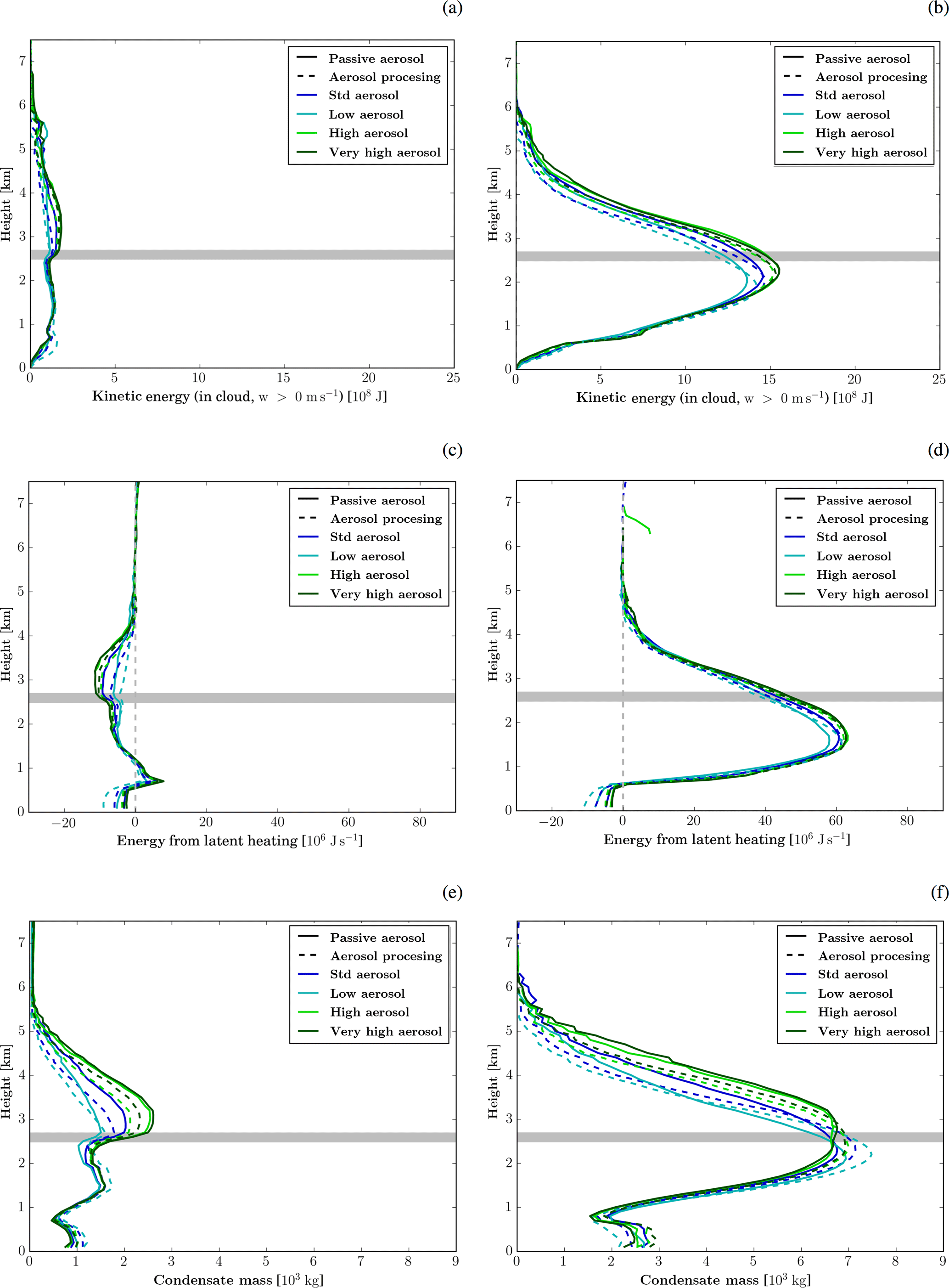
Figure 10Average profiles of (a, b) kinetic energy from vertical velocity, (c, d) latent heat release, and (e, f) condensate content. The left panels shows the average over all columns with a column maximum in-cloud vertical velocity of wmax = 0–3 m s−1 and the right panels for those with wmax > 3 m s−1. The grey horizontal line indicates the location of the 0∘C level.
6.2 Aerosol impact on convective core and stratiform regions
For a closer analysis of the changes in condensate gain and loss, the cloud field is decomposed into regions with different updraft strength. Cloudy columns are stratified according to the column maximum in-cloud vertical velocity at each grid point (wmax). In-cloud grid points have a minimum condensate content of 1 mg kg−1. ΔG for the conditionally sampled areas of the domain is shown in Fig. 9a. Condensation changes are dominated by regions with large wmax, while smaller changes in opposite sign occur in weaker-updraft regions. In contrast, weak-updraft regions contribute most to changes in deposition. These modifications go along with changes in the vertical extent and area covered by the updraft regions (Fig. 9b, Fig. S18a). Updraft cores deepen by about 100–150 m for each factor of 10 increase in aerosol number concentration, while the areal extent increases by about 25 %. These changes in the updraft geometry contribute to the differences in column-integrated condensate generation between simulations. However, they do not fully explain them, since the volume-averaged condensation rate also increases with aerosol concentration (Fig. S18b). These changes are consistent between simulations with and without aerosol processing.
Different responses to aerosol perturbations are expected in the convective core regions and the more stratiform regions of the cells. Based on the change in sign of ΔG between regions with a column maximum velocity wmax = 3 m s−1 and , we define updraft regions by and more stratiform regions by . Average profiles of kinetic energy, latent heating rates, and total condensed water for the two regions are shown in Fig. 10.
In the convective core regions, the kinetic energy and the latent heat release increases with increasing aerosol concentrations (Fig. 10b, d). Both of these variables peak in the warm-phase part of the cloud. The peak in kinetic energy occurs about 1 km above the peak in latent heat release. The maximum in both variables shifts to higher altitudes with increasing aerosol concentrations. Latent heat release above the 0∘C level increases slightly for higher-aerosol scenarios, but the changes are very small compared to those below the 0∘C level. The generally small changes above the 0∘C level indicate that the precipitation enhancement is mainly a result of changes in the warm-phase part of the cloud, as suggested by the analysis in Sect. 6.1. While energy released from phase transitions below 2 km altitude increases with increasing aerosol number concentrations (Fig. 10f), the vertical velocity is almost unaltered (Fig. 10b) as is the cloud base temperature (, not shown). Therefore, we hypothesise that the higher condensation rates are due to less dry air being mixed into the high-updraft regions for increasing aerosol conditions. The reduced impact of mixing with drier air would be consistent with on average larger cells and an increasing stratiform area (Figs. 5b, 9b). The stronger latent heating from convection as well as the weaker mixing with low kinetic energy air masses (due to a wider updraft region) contributes to the higher vertical velocities aloft. The larger vertical motion promotes the upward transport of condensate. The condensate mass in the lower parts of the cloud decreases with increasing aerosol, while it increases above the 0∘C level (Fig. 10f). The altitude of the maximum condensate loading also shifts to higher altitudes for higher aerosol loadings. The higher condensate amounts towards cloud top are also supported by slower conversion rates of cloud condensate into rain with increasing aerosol concentration (Fig. S19). In contrast, condensate mass increases with decreasing aerosol number concentrations in the lower parts of the clouds. This is mainly a result of the sedimentation of rain, which is more efficiently produced in low-aerosol conditions. No further increase in latent heating, kinetic energy, or condensate content occurs for an increase beyond the high-aerosol scenario.
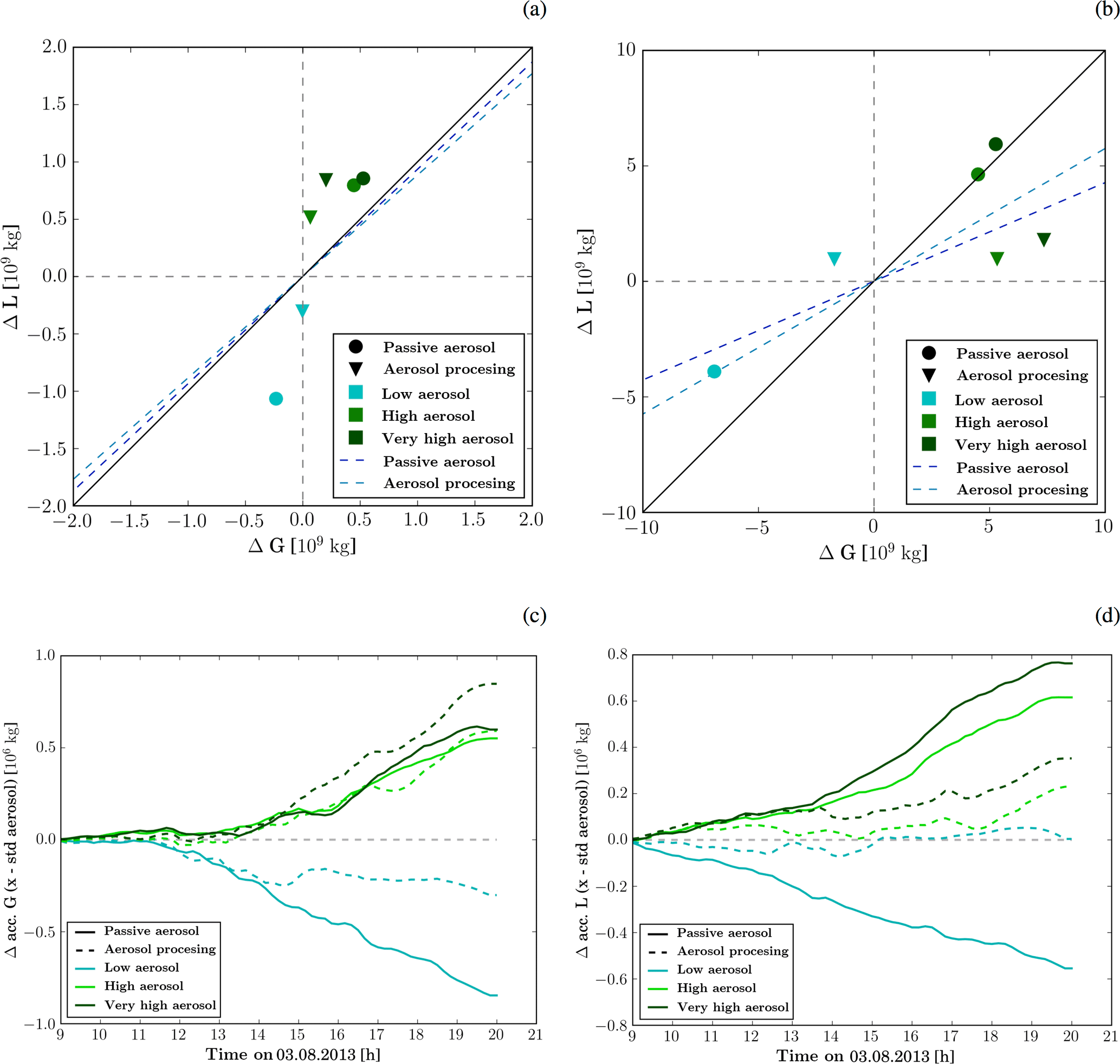
Figure 11The panels in the upper row show ΔG in relation to ΔL for the time period between (a) 09:00–12:00 UTC and (b) 12:00–21:00 UTC. The panels in the lower row show the difference in (c) accumulated condensate generation and (d) condensate loss relative to the simulation with standard-aerosol profile. Solid lines represent simulations with passive aerosols and dashed lines those with aerosol processing.
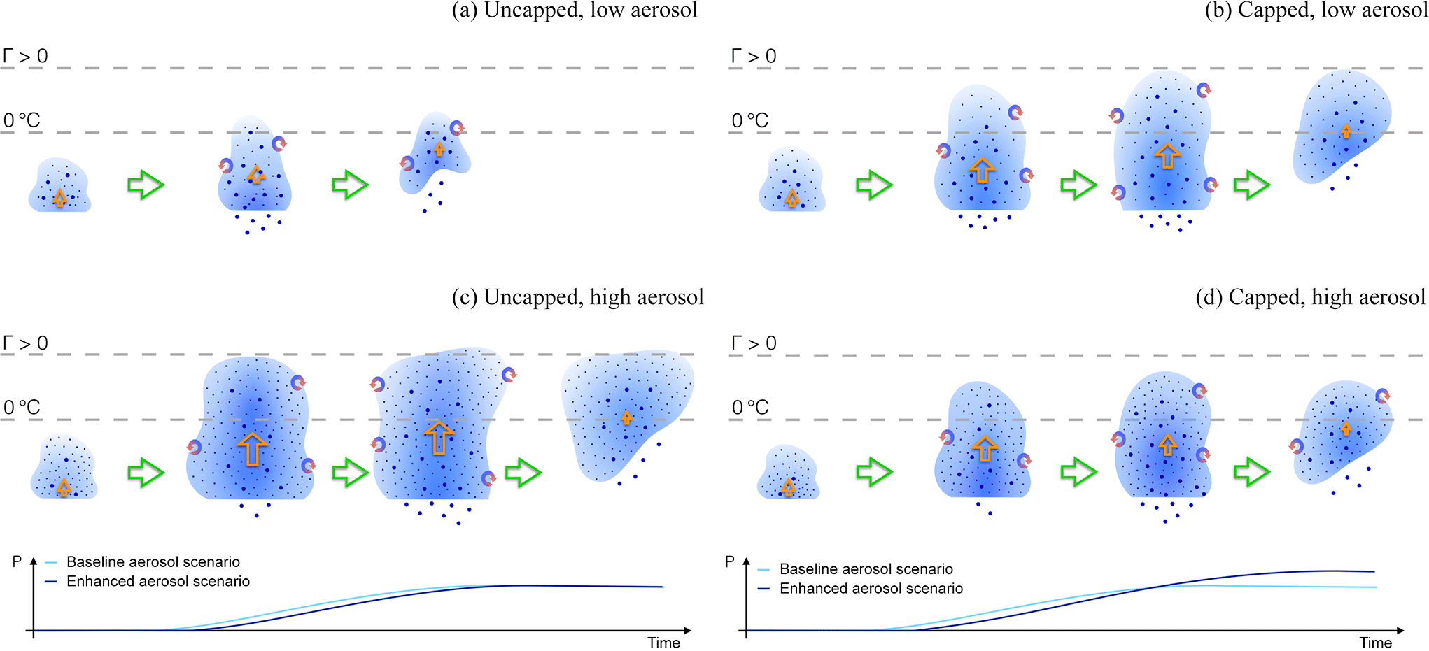
Figure 12Schematic summary of aerosol-induced changes in the investigated clouds for a scenario in which cloud tops are not limited by an upper-level stable layer (a, c) and one in which they are (b, d). The cloud evolution in a low-aerosol environment is illustrated in (a, b) and in a high-aerosol environment in (c, d). The intensity of the shading indicates the condensate mass mixing ratio. Small dots represent cloud droplets and larger ones rain drops. Different stages during the cloud evolution are depicted from left to right and the lower section of each panel shows the time series of accumulated precipitation from each cloud (cyan: baseline aerosol, dark blue: enhanced aerosol). The orange arrows indicate vertical velocity in the convective core region.
In the stratiform region, the kinetic energy in the lower parts of the clouds is not affected by modified aerosol concentrations, while it increases with increasing aerosol concentrations higher up (Fig. 10a). With increasing aerosol concentrations, the latent heat release close to cloud base slightly increases. In contrast, the latent heating becomes more negative in the upper part of the clouds (Fig. 10c). The condensed water content also shows a small increase close to cloud base, little change up to 2 km, and a strong increase aloft (Fig. 10e). The changes in the upper parts of the clouds are most likely due to a larger horizontal transport of condensed water into the stratiform regions of the clouds. This may be caused by a stronger divergence in the upper parts of the clouds in direct consequence of a higher vertical flux in the convective core region. Also, it is expected that the higher condensate content in the upper parts of the clouds enables lateral mixing to broaden the cloud. In contrast, for low condensate conditions lateral mixing most likely leads to the evaporation of the cloud. The hypothesis of a broadening of the clouds by larger transport into the stratiform regions is consistent with the overall larger cloud size in the scenarios with higher aerosol concentrations (Fig. 5b). Furthermore, reduced lateral mixing would result in a weaker impact of entrainment of dry air into the convective core regions supporting the formation of wider and deeper regions as discussed before. The increase in condensate loading in the stratiform region is particularly pronounced for simulations in which vertical growth of the clouds is prohibited by the stable layer aloft (high-aerosol scenario with passive aerosols). The enhanced export of condensate to the stratiform region together with a less efficient rain and graupel production (Fig. S19) likely contributes to a reduction in PE. The reduced PE impedes a further increase in surface precipitation.
The discussed changes in cloud dynamics and microphysics are consistent between simulations with passive aerosol and aerosol processing. The difference between the passive-aerosol and aerosol-processing simulations can be understood based on the same physical mechanism when taking into account the overall lower CDNC and lower cloud tops for the same aerosol scenario.
6.3 Transition from precipitation suppression to enhancement
The discussion in the previous two sections focused on the precipitation enhancement with increasing aerosol concentrations during the period of main convective activity (12:00–20:00 UTC). However, in the earlier period with scattered convection, precipitation is suppressed by higher aerosol concentrations (Sect. 5.2). In the morning, the average cloud depth is smaller and cloud top height shows only little sensitivity to aerosol perturbations (Fig. 5d, Fig. S20a). The clouds are predominantly warm phase with very small amounts of ice-phase particles close to cloud top. Consistent with the small change in cloud top height, the condensate gain displays only minor changes. Changes in the condensate loss are more significant and, in contrast to the clouds developing later, dominate the condensate budget (Fig. 11). Changes in mean cell size are much smaller in magnitude than later on in the day (Fig. 5b). The lack of ice-phase species and the lower wind speeds at cloud top (not shown) limit the lateral transport of condensate into the area surrounding the updraft core and thereby prevent cells from growing larger. Accordingly, the main control on the precipitation formation is the efficiency of cloud microphysical processes in producing precipitation-sized hydrometeors (Fig. 11a). It is known from parcel model studies that the efficiency of the cloud condensate to precipitation conversion process rapidly increases with decreasing CDNC and hence aerosol concentrations.
In contrast, as clouds organise along the sea-breeze fronts and become on average deeper later in the day (Fig. 5a, Fig. S20b), changes in the condensate gain become more important. Maximum in-cloud vertical velocities often exceed 3 m s−1, a larger mixed-phase region develops, and the cloud depth and cell width is more sensitive to the aerosol scenario. The change in surface precipitation in the early period is mainly driven by weak-updraft regions (Fig. S21a). After the transition to organised convection, regions with larger updraft velocities contribute to the precipitation response. Also, the precipitation response in the weak-updraft regions changes sign. The shift from precipitation decrease to increase in the weak-updraft regions is likely associated with a large increase in the condensed water path in the later period (Fig. S21c to f). We hypothesise that this is due to the added impact of lateral transport from the convective core regions into the more stratiform regions (Fig. 10e and Sect. 6.2).
While the sign of the precipitation change is consistent for all vertical velocity regions in the aerosol-processing runs, for simulations with passive aerosol the medium-updraft regions () show a precipitation change opposite to the weak and strong-updraft regions (Fig. S21b). This is particularly important for the high and very high-aerosol scenario, for which the total precipitation response is dominated by the medium-updraft regions. Importantly, the precipitation from the convective core region does not increase further for high or very high-aerosol scenarios. As discussed earlier (see Sect. 6.2), we hypothesise that the thermodynamic limits on cloud deepening is responsible for this behaviour.
The main driver for the transition from precipitation suppression to precipitation enhancement therefore is the larger forcing of the convective clouds by the sea-breeze convergence zone which influences the cloud depth and horizontal structure of the cloud field.
The aerosol-induced changes in cloud structure, life cycle, and precipitation formation for the phase of organised convection are summarised in Fig. 12. The right (left) column corresponds to clouds for which the vertical development is (not) limited by a stable layer aloft. The upper panels depict the control scenario, while the lower panels show the cloud evolution under increased aerosol conditions.
Aerosol–cloud interactions are investigated for mixed-phase convective clouds developing along a sea-breeze convergence zone over the southwestern peninsula of the UK. High-resolution (Δx = 250 m) simulations with the Unified Model have been conducted with a newly developed cloud microphysics scheme (CASIM), which can represent the modification of the aerosol environment by cloud microphysical processes. Evaluation of the model simulations with observations from the COPE campaign suggests a good model performance in terms of the thermodynamic, cloud, cloud microphysical, and radar reflectivity structures. The good agreement with low-level radar reflectivity but larger difference in surface precipitation rate may point either to issues with the assumptions used for the reflectivity diagnostics in the model or potential issues with the radar-retrieved surface precipitation rates.
A novel aspect of CASIM is the representation of modifications to the aerosol environment by cloud microphysical processes in a numerical weather prediction framework. Including this feedback has a largely positive impact on the model performance in terms of cloud base cloud droplet number density and radar reflectivity but leads to a stronger underestimation of domain-average surface precipitation and average cell sizes. The most important impacts of including aerosol processing for cloud properties and aerosol-induced changes thereof are as follows:
-
Aerosol processing reduces cloud base CDNC, results in a more rapid decrease in CDNC with altitude, and increases the spread of CDNC values at each altitude.
-
In the period with unorganised convection, aerosol processing reduces the amplitude of the precipitation suppression with increasing aerosol compared to simulations with passive aerosol.
-
Precipitation changes in the second period with organised convection are larger when aerosol processing is included. The larger signal is due to on average lower cloud tops with a larger potential for cloud deepening and a larger PE for high-aerosol scenarios. For passive aerosols, small reductions in PE occur for increasing aerosol.
The two-way interaction between clouds and aerosols is an important feedback mechanism, which may impact the magnitude of aerosol-induced changes in clouds and is one source for co-variability between cloud and aerosol fields. The modification of the aerosol size distribution and number density by cloud microphysics has been studied in laboratory experiments (Mitra et al., 1992) and documented in aircraft campaigns (Yang et al., 2015). Its importance has been demonstrated in several modelling studies for orographic clouds (Pousse-Nottelmann et al., 2015; Xue et al., 2010) and stratocumulus clouds (Feingold et al., 1996). The impact of aerosol–cloud co-variability is particularly important on larger spatial and temporal scales, which typically cannot be represented in very high-resolution simulations with detailed bin microphysics. Hence, one-way (aerosol impact on cloud field) or two-way coupling (aerosol impact on cloud field and vice versa) between aerosol and cloud fields has been implemented in some numerical weather prediction models with bulk microphysics schemes (e.g. COSMO-ART, Consortium for Small-scale Modeling model coupled to the Aerosols and Reactive Trace gases model, Vogel et al., 2009; COSMO-MUSCAT, COSMO model coupled to the Multi-Scale Chemistry Aerosol Transport model, Dipu et al., 2017; or WRF-Chem, Weather Research and Forecasting model coupled with Chemistry, Fast et al., 2006). Notwithstanding the recent development of these modelling systems, only a limited number of studies on the sensitivity of cloud–aerosol interactions are available. The published studies predominantly focus on aerosol processing in stratocumulus clouds. In this work we have shown the importance of aerosol processing in mixed-phase convection along sea-breeze fronts.
Perturbations to the aerosol initial and boundary conditions (modifications by factors of 0.1, 10, and 30) cause changes in the cloud microphysical properties, geometry, and precipitation production in the case analysed here. These changes are summarised in Fig. 12. Key aspects are listed as follows:
-
Aerosol perturbations modify the cell number and sizes but have little impact on the domain cloud fraction.
-
Changes in the cloud field structure and presumably associated changes in lateral mixing are important for the response to aerosol perturbations.
-
Precipitation suppression under high-aerosol conditions transitions to precipitation enhancement when the clouds organise and on average grow deeper.
-
Changes in precipitation are mainly a result of modified condensate gain in the warm-phase part of the clouds. Changes in PE support the precipitation enhancement for simulations with aerosol processing but act in the opposite direction for simulations with passive aerosol.
-
The enhanced condensate gain is due to changes in the convective core region, where vertical velocities and latent heat release from condensation increase.
-
The enhanced condensate gain is not translated into a precipitation enhancement when clouds grow into an upper-level stable layer limiting cloud depth.
The change in the sign of the precipitation response from shallower unorganised to deeper and more organised convection is in line with previous results from individual simulations (summarised for example by Khain, 2009). Different precipitation responses for convective and for more stratiform precipitation have also been documented in the large domain simulations of tropical convection by Lee and Feingold (2010). Previous studies on aerosol-induced changes in precipitation formation in deep convective clouds mainly focussed on changes in latent heating in the mixed-phase part of the clouds (Lebo and Seinfeld, 2011; Rosenfeld et al., 2008). In contrast, our simulations suggest that the precipitation response is mainly driven by changes in latent heating below the 0∘C level. The idealised studies of Sheffield et al. (2015) and Lebo (2014) have also found changes in the warm-phase section of the clouds to dominate over latent heating changes in the mixed-phase part. The increase in warm-phase latent heating in Sheffield et al. (2015) and Lebo (2014) is due to a more efficient vapour deposition on the more numerous cloud droplets in polluted conditions. This mechanism cannot be represented in our modelling system, as we use a saturation adjustment scheme. In contrast, we hypothesise that the changes in latent heating rates from condensation are related to changes in the horizontal cloud field structure. Interestingly, Lebo (2017) showed with a simplified modelling system that temperature perturbations in the warm-phase section of convective clouds have a larger potential to increase the updraft strength compared to temperature perturbations in the mixed-phase section. Changes in horizontal cloud structure have received less attention in previous studies compared to the more frequently analysed changes in cloud top height (Koren et al., 2005; Morrison and Grabowski, 2011; Stevens and Feingold, 2009). Most previous studies used either small domain, high-resolution simulations unable to represent large changes in cloud field structure or larger domain but coarser resolution simulations lacking a representation of updraft dynamics. In the present study the spatial resolution is high enough to at least partly resolve updraft dynamics and the domain is large enough to represent cloud–cloud interactions as well as to allow for changes in cloud field structure. Our simulations indicate small changes in cloud fraction but major changes in cell number and area. This supports the hypothesised importance of changes in cloud field structure and related compensating mechanisms as suggested for example by Stevens and Feingold (2009).
Despite the fairly high resolution of the presented simulations, there are some issues regarding the representation of lateral mixing in the model simulations. Numerical weather prediction models have known issues with reproducing observed cell size distributions. Also, modelled cell size distributions often do not converge in simulations with increasing spatial resolution (Hanley et al., 2015; Stein et al., 2014, 2015). These problems have been at least partly attributed to the representation of lateral mixing and parameter settings therein (Hanley et al., 2015; Stein et al., 2015). Future studies should investigate the sensitivity of the aerosol-induced changes in cloud field structure to the representation of lateral mixing and test whether similar changes occur in models resolving lateral mixing (LES, large eddy simulations). Other caveats for the presented simulations arise from choices in the microphysical parameterisations. Firstly, the CASIM microphysical module uses the assumption of saturation adjustment. Lebo et al. (2012) found that the representation of supersaturation can lead to significant differences in the magnitude of aerosol-induced changes in latent heating in the mixed-phase part of clouds. Changes in latent heating were found to be much smaller if saturation adjustment was used. Secondly, the representation of mixed-phase cloud microphysics in models has a number of uncertainties of parametric and structural nature. These include, but are not limited to, the representation of primary and secondary ice formation, drop freezing, rimed particle density, and diameter–fall-speed relations (Huang et al., 2017; Johnson et al., 2015; Morrison, 2012). Most of these uncertainties in the microphysics are expected to influence the precipitation efficiency. However, given that changes in condensate generation play an important role in the studied clouds, it can be speculated that these changes may have an impact on the overall precipitation but not on the mechanism of the precipitation response.
In the second part of this study, we will investigate how the aerosol-induced changes in cloud structure and precipitation compare to uncertainties in meteorological initial conditions. We will also assess whether the aerosol-induced changes are consistent in sign and amplitude across the initial condition ensemble. This will provide insight into the detectability of aerosol–cloud interactions in observational data and the demands on observational data to enable a detection of aerosol-induced changes.
Model data are stored on the tape archive provided by the JASMIN (http://www.jasmin.ac.uk/, last access: March 2018) service. Data access to Met Office data via JASMIN is described at http://www.ceda.ac.uk/blog/access-to-the-met-office-mass-archive-on-jasmin-goes-live/ (last access: March 2018).
The surface precipitation P equals the difference between condensate generation G (condensation and deposition) and condensate loss L (evaporation and sublimation) in a mass conserving system with no change in condensate storage:
The condensate generation is mainly determined by the cloud dynamics, i.e. uplift in saturated conditions, and to a smaller extend the efficiency with which the generated supersaturation is depleted by transfer to the condensed phase. The condensate loss is determined by the efficiency of microphysical processes in converting condensate to surface precipitation and the timescale available for this conversion, i.e. the residence time of any infinitely small air parcels in (super-)saturated conditions. Accordingly the change in precipitation between two different cases is the result of changes in the generation and loss terms. If the changes in loss are larger than those in the generation term, precipitation will decrease and vice-versa. A convenient way to display this analysis is therefore a plot of ΔG against ΔL (Fig. A1).
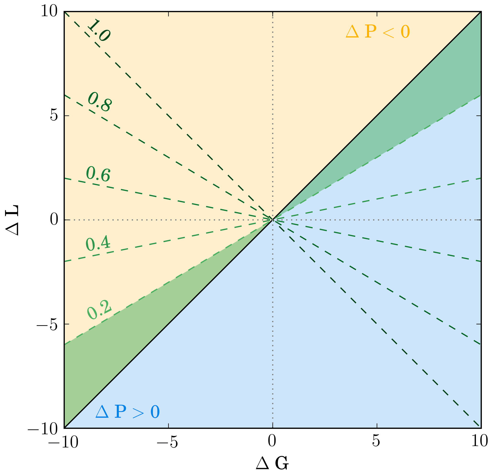
Figure A1Exemplary ΔG versus ΔL diagram as explained in Appendix A. In simulations falling into the yellow (blue) shaded area less (more) precipitation is formed than in the reference. The change in precipitation is dominated by ΔG for simulations in the green shaded area, while precipitation changes in the rest of the phase space are dominated by changes in PE. For example the green shaded area illustrates an assumed PE of 0.2 for the reference simulation. For other values of PE, the area is bounded by the black solid line and the respective green dashed lines.
This analysis can be extended to address the question of whether a specific change in surface precipitation is dominated by a change in the generation term or a change in the conversion efficiency. For this purpose, the precipitation efficiency is used, which is defined as the ratio of surface precipitation to condensate generation. The change in surface precipitation can be decomposed according to
The terms with subscript “ctr” refer to the simulation with the control aerosol scenario and those with subscript “per” to the simulation with a perturbed aerosol scenario. The first term on the right side of the equation quantifies the contribution of a change in generation and the second term those of an altered PE. The conditions for which the change in condensate generation dominate are accordingly
These conditions are met by the following combinations of ΔG and ΔL:
The respective areas in the ΔG−ΔL are illustrated in Fig. A1.
The supplement related to this article is available online at: https://doi.org/10.5194/acp-18-3119-2018-supplement.
All authors contributed to the development of the concepts and ideas presented in this paper. BJS developed the CASIM microphysics code. AAH, JMW, PRF, and AKM contributed to the further development of the CASIM code. AKM, PR, and PRF helped set up the model runs. RS provided the 3-D radar composite. PR compiled and analysed the aircraft data set. AMB provided expertise on the observational data sets and the observational campaign. AKM performed the model simulations and model analysis and wrote the majority of the manuscript, along with input and comments from all co-authors.
The authors declare that they have no conflict of interest.
We thank the COPE research team for collecting observational data and in
particular John Taylor from the University of Manchester for discussion
related to the cloud droplet data. Further, we acknowledge the use of the
MONSooN system, a collaborative facility supplied under the Joint Weather and
Climate Research Programme, a strategic partnership between the Met Office
and the Natural Environment Research Council. Further we acknowledge JASMIN
storage facilities (https://doi.org/10.1109/BigData.2013.6691556), FAAM, NCAS AMF (Atmospheric Measurement Facility), CEDA, BADC,
and the Radarnet at the Met Office team for providing data. The University of
Leeds is acknowledged for providing funds for this study. We thank two
anonymous reviewers for their valuable feedback.
Edited by: Johannes Quaas
Reviewed by: two
anonymous referees
Abdul-Razzak, H. and Ghan, S. J.: A parameterization of aerosol activation. 2. Multiple aerosol types, J. Geophys. Res., 105, 6837–6844, 2000. a, b
Abdul-Razzak, H., Ghan, S. J., and Rivera-Carpio, C.: A parameterization of aerosol activation. 1. Single aerosol type, J. Geophys. Res., 103, 6123–6131, 1998. a, b
Albrecht, B. A.: Aerosols, cloud microphysics, and fractional cloudiness, Science, 245, 1227–1230, https://doi.org/10.1126/science.245.4923.1227, 1989. a, b
Altaratz, O., Koren, I., Remer, L. A., and Hirsch, E.: Review: Cloud invigoration by aerosols – coupling between microphysics and dynamics, Atmos. Res., 140–141, 38–60, https://doi.org/10.1016/j.atmosres.2014.01.009, 2014. a, b, c
Andreae, M. O.: Correlation between cloud condensation nuclei concentration and aerosol optical thickness in remote and polluted regions, Atmos. Chem. Phys., 9, 543–556, https://doi.org/10.5194/acp-9-543-2009, 2009. a
Aranami, K., Zerroukat, M., and Wood, N.: Mixing properties of SLICE and other mass-conservative semi-Lagrangian schemes, Q. J. Roy. Meteorol. Soc., 140, 2084–2089, https://doi.org/10.1002/qj.2268, 2014. a, b
Aranami, K., Davies, T., and Wood, N.: A mass restoration scheme for limited-area models with semi-Lagrangian advection, Q. J. Roy. Meteorol. Soc., 141, 1795–1803, https://doi.org/10.1002/qj.2482, 2015. a, b
Barstad, I., Grabowski, W. W., and Smolarkiewicz, P. K.: Characteristics of large-scale orographic precipitation: Evaluation of linear model in idealized problems, J. Hydrol., 340, 78–90, https://doi.org/10.1016/j.jhydrol.2007.04.005, 2007. a
Bigg, E. K.: The formation of atmospheric ice crystals by the freezing of droplets, Q. J. Roy. Meteorol. Soc., 39, 510–519, https://doi.org/10.1002/qj.49707934207, 1953. a
Blyth, A. M., Bennett, L. J., and Collier, C. G.: High-resolution observations of precipitation from cumulonimbus clouds, Meteorol. Appl., 22, 75–89, https://doi.org/10.1002/met.1492, 2015. a, b
Comin, A. N., Miglietta, M. M., Rizza, U., Acevedo, O. C., and Degrazia, G. A.: Investigation of sea-breeze convergence in Salento Peninsula (southeastern Italy), Atmos. Res., 160, 68–79, https://doi.org/10.1016/j.atmosres.2015.03.010, 2015. a
Cui, Z., Davies, S., Carslaw, K. S., and Blyth, A. M.: The response of precipitation to aerosol through riming and melting in deep convective clouds, Atmos. Chem. Phys., 11, 3495–3510, https://doi.org/10.5194/acp-11-3495-2011, 2011. a, b
DeMott, P. J., Prenni, A. J., Liu, X., Kreidenweis, S. M., Petters, M. D., Twohy, C. H., Richardson, M. S., Eidhammer, T., and Rogers, D. C.: Predicting global atmospheric ice nuclei distributions and their impacts on climate, P. Natl. Acad. Sci. USA, 107, 11217–11222, https://doi.org/10.1073/pnas.0910818107, 2010. a, b
Devasthale, A., Kruger, O., and Grassl, H.: Change in cloud-top temperatures over Europe, IEEE Geosci. Remote Sens. Lett., 2, 333–336, https://doi.org/10.1109/LGRS.2005.851736, 2005. a
Dipu, S., Quaas, J., Wolke, R., Stoll, J., Mühlbauer, A., Sourdeval, O., Salzmann, M., Heinold, B., and Tegen, I.: Implementation of aerosol-cloud interactions in the regional atmosphere-aerosol model COSMO-MUSCAT(5.0) and evaluation using satellite data, Geosci. Model Dev., 10, 2231–2246, https://doi.org/10.5194/gmd-10-2231-2017, 2017. a
Fan, J., Zhang, R., Li, G., and Tao, W.-K.: Effects of aerosols and relative humidity on cumulus clouds, J. Geophys. Res.-Atmos., 112, D14204, https://doi.org/10.1029/2006JD008136, 2007. a
Fan, J., Yuan, T., Comstock, J. M., Ghan, S., Khain, A., Leung, L. R., Li, Z., Martins, V. J., and Ovchinnikov, M.: Dominant role by vertical wind shear in regulating aerosol effects on deep convective clouds, J. Geophys. Res.-Atmos., 114, D22206, https://doi.org/10.1029/2009JD012352, 2009. a
Fan, J., Leung, L. R., Li, Z., Morrison, H., Chen, H., Zhou, Y., Qian, Y., and Wang, Y.: Aerosol impacts on clouds and precipitation in eastern China: Results from bin and bulk microphysics, J. Geophys. Res.-Atmos., 117, D00K36, https://doi.org/10.1029/2011JD016537, 2012. a, b, c, d, e
Fast, J. D., Gustafson, W. I., Easter, R. C., Zaveri, R. A., Barnard, J. C., Chapman, E. G., Grell, G. A., and Peckham, S. E.: Evolution of ozone, particulates, and aerosol direct radiative forcing in the vicinity of Houston using a fully coupled meteorology-chemistry-aerosol model, J. Geophys. Res.-Atmos., 111, D21305, https://doi.org/10.1029/2005JD006721, 2006. a
Feingold, G., Kreidenweis, S. M., Stevens, B., and Cotton, W. R.: Numerical simulations of stratocumulus processing of cloud condensation nuclei through collision-coalescence, J. Geophys. Res.-Atmos., 101, 21391–21402, https://doi.org/10.1029/96JD01552, 1996. a
Feingold, G., McComiskey, A., Rosenfeld, D., and Sorooshian, A.: On the relationship between cloud contact time and precipitation susceptibility to aerosol, J. Geophys. Res.-Atmos., 118, 10544–10554, https://doi.org/10.1002/jgrd.50819, 2013. a
Feingold, G., McComiskey, A., Yamaguchi, T., Johnson, J. S., Carslaw, K. S., and Schmidt, K. S.: New approaches to quantifying aerosol influence on the cloud radiative effect, P. Natl. Acad. Sci. USA, 113, 5812–5819, https://doi.org/10.1073/pnas.1514035112, 2016. a
Flossmann, A. I., Hall, W. D., and Pruppacher, H. R.: A theoretical study of the wet removal of atmospheric pollutants. Part I: The redistribution of aerosol particles captured through nucleation and impaction scavenging by growing cloud drops, J. Atmos. Sci., 42, 583–606, https://doi.org/10.1175/1520-0469(1985)042<0583:ATSOTW>2.0.CO;2, 1985. a
Golding, B., Clark, P., and May, B.: The Boscastle flood: Meteorological analysis of the conditions leading to flooding on 16 August 2004, Weather, 60, 230–235, https://doi.org/10.1256/wea.71.05, 2005. a
Grant, L. D. and van den Heever, S. C.: Aerosol-cloud-land surface interactions within tropical sea breeze convection, J. Geophys. Res., 119, 8340–8361, https://doi.org/10.1002/2014JD021912, 2014. a
Grosvenor, D. P., Field, P. R., Hill, A. A., and Shipway, B. J.: The relative importance of macrophysical and cloud albedo changes for aerosol-induced radiative effects in closed-cell stratocumulus: insight from the modelling of a case study, Atmos. Chem. Phys., 17, 5155–5183, https://doi.org/10.5194/acp-17-5155-2017, 2017. a
Gryspeerdt, E., Stier, P., and Partridge, D. G.: Links between satellite-retrieved aerosol and precipitation, Atmos. Chem. Phys., 14, 9677–9694, https://doi.org/10.5194/acp-14-9677-2014, 2014. a
Halliwell, C.: Subgrid turbulence scheme, Unified Model documentation paper 028, Met Office, 2015. a
Hanley, K. E., Plant, R. S., Stein, T. H. M., Hogan, R. J., Nicol, J. C., Lean, H. W., Halliwell, C., and Clark, P. A.: Mixing-length controls on high-resolution simulations of convective storms, Q. J. Roy. Meteorol. Soc., 141, 272–284, https://doi.org/10.1002/qj.2356, 2015. a, b, c
Harrison, D. L., Scovell, R. W., and Kitchen, M.: High-resolution precipitation estimates for hydrological uses, Proceedings of the Institution of Civil Engineers – Water Management, 162, 125–135, https://doi.org/10.1680/wama.2009.162.2.125, 2009. a, b
Hill, A. A., Shipway, B. J., and Boutle, I. A.: How sensitive are aerosol-precipitation interactions to the warm rain representation?, J. Adv. Model. Earth Syst., 7, 987–1004, https://doi.org/10.1002/2014ms000422, 2015. a, b, c
Huang, Y., Blyth, A. M., Brown, P. R. A., Choularton, T. W., and Cui, Z.: Factors controlling secondary ice production in cumulus clouds, Q. J. Roy. Meteorol. Soc., 143, 1021–1031, https://doi.org/10.1002/qj.2987, 2017. a
Johnson, J. S., Cui, Z., Lee, L. A., Gosling, J. P., Blyth, A. M., and Carslaw, K. S.: Evaluating uncertainty in convective cloud microphysics using statistical emulation, J. Adv. Model. Earth Syst., 7, 162–187, https://doi.org/10.1002/2014MS000383, 2015. a, b, c
Khain, A. and Lynn, B.: Simulation of a supercell storm in clean and dirty atmosphere using weather research and forecast model with spectral bin microphysics, J. Geophys. Res.-Atmos., 114, D19209, https://doi.org/10.1029/2009JD011827, 2009. a, b, c, d, e
Khain, A., Pokrovsky, A., Pinsky, M., Seifert, A., and Phillips, V.: Simulation of effects of atmospheric aerosols on deep turbulent convective clouds using a spectral microphysics mixed-phase cumulus cloud model. Part I: model description and possible applications, J. Atmos. Sci., 61, 2963–2982, 2004. a, b
Khain, A., Rosenfeld, D., and Pokrovsky, A.: Aerosol impact on the dynamics and microphysics of deep convective clouds, Q. J. Roy. Meteorol. Soc., 131, 2639–2663, https://doi.org/10.1256/qj.04.62, 2005. a
Khain, A. P.: Notes on state-of-the-art investigations of aerosol effects on precipitation: A critical review, Environ. Res. Lett., 4, 015004, https://doi.org/10.1088/1748-9326/4/1/015004, 2009. a, b, c
Khain, A. P., Beheng, K. D., Heymsfield, A., Korolev, A., Krichak, S. O., Levin, Z., Pinsky, M., Philips, V., Prabhakaran, T., Teller, A., van den Heever, S. C., and Yano, J.-I.: Representation of microphysical processes in cloud-resolving models: spectral (bin) microphysics vs. bulk parameterization, Rev. Geophys., 53, 247–322, https://doi.org/10.1002/2014RG000468, 2015. a
Koren, I., Kaufman, Y. J., Rosenfeld, D., Remer, L. A., and Rudich, Y.: Aerosol invigoration and restructuring of Atlantic convective clouds, Geophys. Res. Lett., 32, L14828, https://doi.org/10.1029/2005GL023187, 2005. a, b
Koren, I., Feingold, G., and Remer, L. A.: The invigoration of deep convective clouds over the Atlantic: aerosol effect, meteorology or retrieval artifact?, Atmos. Chem. Phys., 10, 8855–8872, https://doi.org/10.5194/acp-10-8855-2010, 2010. a
Lakshmanan, V., Hondl, K., Potvin, C. K., and Preignitz, D.: An improved method for estimating radar echo-top height, Weather Forecast., 28, 481–488, https://doi.org/10.1175/WAF-D-12-00084.1, 2013. a
Lebo, Z.: A numerical investigation of the potential effects of aerosol-induced warming and updraft width and slope on updraft intensity in deep convective clouds, J. Atmos. Sci., 75, 535–554, https://doi.org/10.1175/JAS-D-16-0368.1, 2017. a
Lebo, Z. J.: The Sensitivity of a Numerically Simulated Idealized Squall Line to the Vertical Distribution of Aerosols, J. Atmos. Sci., 71, 4581–4596, https://doi.org/10.1175/JAS-D-14-0068.1, 2014. a, b, c
Lebo, Z. J. and Morrison, H.: Dynamical effects of aerosol perturbations on simulated idealized squall lines, Mon. Weather Rev., 142, 991–1009, https://doi.org/10.1175/MWR-D-13-00156.1, 2014. a, b
Lebo, Z. J. and Seinfeld, J. H.: Theoretical basis for convective invigoration due to increased aerosol concentration, Atmos. Chem. Phys., 11, 5407–5429, https://doi.org/10.5194/acp-11-5407-2011, 2011. a, b, c, d
Lebo, Z. J., Morrison, H., and Seinfeld, J. H.: Are simulated aerosol-induced effects on deep convective clouds strongly dependent on saturation adjustment?, Atmos. Chem. Phys., 12, 9941–9964, https://doi.org/10.5194/acp-12-9941-2012, 2012. a, b, c
Lee, S. S.: Effect of aerosol on circulations and precipitation in deep convective clouds, J. Atmos. Sci., 69, 1957–1974, https://doi.org/10.1175/JAS-D-11-0111.1, 2012. a
Lee, S.-S. and Feingold, G.: Precipitating cloud-system response to aerosol perturbations, Geophys. Res. Lett., 37, L23806, https://doi.org/10.1029/2010GL045596, 2010. a, b
Leon, D. C., French, J. R., Lasher-Trapp, S., Blyth, A. M., Abel, S. J., Ballard, S., Barrett, A., Bennett, L. J., Bower, K., Brooks, B., Brown, P., Charlton-Perez, C., Choularton, T., Clark, P., Collier, C., Crosier, J., Cui, Z., Dey, S., Dufton, D., Eagle, C., Flynn, M. J., Gallagher, M., Halliwell, C., Hanley, K., Hawkness-Smith, L., Huang, Y., Kelly, G., Kitchen, M., Korolev, A., Lean, H., Liu, Z., Marsham, J., Moser, D., Nicol, J., Norton, E. G., Plummer, D., Price, J., Ricketts, H., Roberts, N., Rosenberg, P. D., Simonin, D., Taylor, J. W., Warren, R., Williams, P. I., and Young, G.: The Convective Precipitation Experiment (COPE): Investigating the origins of heavy precipitation in the southwestern United Kingdom, B. Am. Meteorol. Soc., 97, 1003–1020, https://doi.org/10.1175/BAMS-D-14-00157.1, 2016. a, b
Li, G., Wang, Y., Lee, K.-H., Diao, Y., and Zhang, R.: Impacts of aerosols on the development and precipitation of a mesoscale squall line, J. Geophys. Res.-Atmos., 114, D17205, https://doi.org/10.1029/2008JD011581, 2009. a
Li, X. and Srivastava, R. C.: An analytical solution for raindrop evaporation and its application to radar rainfall measurements, J. Appl. Meteor., 40, 1607–1616, https://doi.org/10.1175/1520-0450(2001)040<1607:AASFRE>2.0.CO;2, 2001. a
Liang, Z. and Wang, D.: Sea breeze and precipitation over Hainan Island, Q. J. R. Meteorol. Soc., 143, 137–151, https://doi.org/10.1002/qj.2952, 2017. a
Locatelli, J. D. and Hobbs, P. V.: Fall speeds and masses of solid precipitation particles, J. Geophys. Res., 79, 2185–2197, https://doi.org/10.1029/JC079i015p02185, 1974. a
Lock, A., Edwards, J., and Boutle, I.: The parameterisation of boundary layer processes, Unified Model documentation paper 024, Met Office, 2015. a
Lohmann, U. and Feichter, J.: Global indirect aerosol effects: a review, Atmos. Chem. Phys., 5, 715–737, https://doi.org/10.5194/acp-5-715-2005, 2005. a
MetOffice: 1 km Resolution UK Composite Rainfall Data from the Met Office Nimrod System, 2003. a, b
Miller, S. T. K., Keim, B. D., Talbot, R. W., and Mao, H.: Sea breeze: Structure, forecasting, and impacts, Rev. Geophys., 41, 1011, https://doi.org/10.1029/2003RG000124, 2003. a
Miltenberger, A. K., Seifert, A., Joos, H., and Wernli, H.: Scaling relation for warm-phase orographic precipitation – A Lagrangian analysis for 2D mountains, Q. J. Roy. Meteorol. Soc., 141, 2185–2198, https://doi.org/10.1002/qj.2514, 2015. a
Miltenberger, A. K., Field, P. R., Hill, A. A., Shipway, B. J., and Wilkinson, J. M.: Aerosol-cloud interactions in mixed-phase convective clouds. Part 2: Meteorological ensemble, Atmos. Chem. Phys. Discuss., https://doi.org/10.5194/acp-2018-167, in review, 2018.
Mitra, S., Brinkmann, J., and Pruppacher, H.: A wind tunnel study on the drop-to-particle conversion, J. Aerosol Sci., 23, 245–256, https://doi.org/10.1016/0021-8502(92)90326-Q, 1992. a
Morrison, H.: On the robustness of aerosol effects on an idealized supercell storm simulated with a cloud system-resolving model, Atmos. Chem. Phys., 12, 7689–7705, https://doi.org/10.5194/acp-12-7689-2012, 2012. a, b
Morrison, H. and Grabowski, W. W.: Cloud-system resolving model simulations of aerosol indirect effects on tropical deep convection and its thermodynamic environment, Atmos. Chem. Phys., 11, 10503–10523, https://doi.org/10.5194/acp-11-10503-2011, 2011. a, b
NAEI: National Atmospheric Emissions Inventory, available at: http://naei.defra.gov.uk, ©Crown 2017 copyright Defra & BEIS via naei.defra.gov.uk, licenced under the Open Government Licence (OGL), 2014. a
Oguchi, T.: Electromagnetic wave propagation and scattering in rain and other hydrometeors, Proceedings of the IEEE, 71, 1029–1079, 1983. a
Petersen, G. N. and Renfrew, I. A.: Aircraft-based observations of air-sea fluxes over Denmark Strait and the Irminger Sea during high wind speed conditions, Q. J. Roy. Meteorol. Soc., 135, 2030–2045, https://doi.org/10.1002/qj.355, 2009. a
Pousse-Nottelmann, S., Zubler, E. M., and Lohmann, U.: Microphysical processing of aerosol particles in orographic clouds, Atmos. Chem. Phys., 15, 9217–9236, https://doi.org/10.5194/acp-15-9217-2015, 2015. a
Rosenberg, P. D., Dean, A. R., Williams, P. I., Dorsey, J. R., Minikin, A., Pickering, M. A., and Petzold, A.: Particle sizing calibration with refractive index correction for light scattering optical particle counters and impacts upon PCASP and CDP data collected during the Fennec campaign, Atmos. Meas. Tech., 5, 1147–1163, https://doi.org/10.5194/amt-5-1147-2012, 2012. a
Rosenfeld, D., Lohmann, U., Raga, G. B., O'Dowd, C. D., Kulmala, M., Fuzzi, S., Reissell, A., and Andreae, M. O.: Flood or drought: How do aerosols affect precipitation?, Science, 321, 1309–1313, https://doi.org/10.1126/science.1160606, 2008. a, b, c
Rosenfeld, D., Andreae, M. O., Asmi, A., Chin, M., de Leeuw, G., Donovan, D. P., Kahn, R., Kinne, S., Kivekäs, N., Kulmala, M., Lau, W., Schmidt, K. S., Suni, T., Wagner, T., Wild, M., and Quaas, J.: Global observations of aerosol-cloud-precipitation climate interactions, Rev. Geophys., 52, 750–808, https://doi.org/10.1002/2013RG000441, 2014. a
Scovell, R. and al Sakka, H.: A point cloud method for retrieval of high-resolution 3D gridded reflectivity from weather radar networks for air traffic management, J. Atmos. Ocean Tech., 33, 461–479, https://doi.org/10.1175/JTECH-D-15-0051.1, 2016. a, b
Seifert, A. and Beheng, K. D.: A two-moment cloud microphysics parameterization for mixed-phase clouds. Part 2: Maritime vs. continental deep convective storms, Meteorol. Atmos. Phys., 92, 67–82, https://doi.org/10.1007/s00703-005-0113-3, 2006. a
Seifert, A., Köhler, C., and Beheng, K. D.: Aerosol-cloud-precipitation effects over Germany as simulated by a convective-scale numerical weather prediction model, Atmos. Chem. Phys., 12, 709–725, https://doi.org/10.5194/acp-12-709-2012, 2012. a
Sheffield, A. M., Saleeby, S. M., and van den Heever, S. C.: Aerosol-induced mechanisms for cumulus congestus growth, J. Geophys. Res.-Atmos., 120, 8941–8952, https://doi.org/10.1002/2015JD023743, 2015. a, b
Shipway, B. J. and Hill, A. A.: Diagnosis of systematic differences between multiple parametrizations of warm rain microphysics using a kinematic framework, Q. J. Roy. Meteorol. Soc., 138, 2196–2211, https://doi.org/10.1002/qj.1913, 2012. a
Stein, T. H. M., Hogan, R. J., Hanley, K. E., Nicol, J. C., Lean, H. W., Plant, R. S., Clark, P. A., and Halliwell, C. E.: The three-dimensional morphology of simulated and observed convective storms over Southern England, Mon. Weather Rev., 142, 3264–3283, https://doi.org/10.1175/MWR-D-13-00372.1, 2014. a
Stein, T. H. M., Hogan, R. J., Clark, P. A., Halliwell, C. E., Hanley, K. E., Lean, H. W., Nicol, J. C., and Plant, R. S.: The DYMECS project: A statistical approach for the evaluation of convective storms in high-resolution NWP models, B. Am. Meteorol. Soc., 96, 939–951, https://doi.org/10.1175/BAMS-D-13-00279.1, 2015. a, b, c
Stevens, B. and Feingold, G.: Untangling aerosol effects on clouds and precipitation in a buffered system, Nature, 461, 607–613, https://doi.org/10.1038/nature08281, 2009. a, b, c
Stevens, B. and Seifert, A.: Understanding macrophysical outcomes of microphysical choices in simulations of shallow cumulus convection, J. Meteor. Soc. Jap., 86A, 143–162, https://doi.org/10.2151/jmsj.86A.143, 2008. a
Stocker, T., Qin, D., Plattner, G.-K., Tignor, M., Allen, S., Boschung, J., Nauels, A., Xia, Y., Bex, V., and Midgley, P. (Eds.): Climate change 2013: The physical science basis. Contribution of Working Group I to the Fifth Assessment Report of the Intergovernmental Panel on Climate Change, Cambridge University Press, Cambridge, United Kingdom and New York, NY, USA, 2013. a, b
Stratton, R., Willet, M., Derbyshire, S., Wong, R., and Whitall, M.: Convection schemes, Unified Model documentation paper 027, Met Office, 2015. a
Tao, W.-K., Li, X., Khain, A., Matsui, T., Lang, S., and Simpson, J.: Role of atmospheric aerosol concentration on deep convective precipitation: Cloud-resolving model simulations, J. Geophys. Res.-Atmos., 112, D24S18, https://doi.org/10.1029/2007JD008728, 2007. a, b
Tao, W.-K., Chen, J.-P., Li, Z., Wang, C., and Zhang, C.: Impact of aerosols on convective clouds and precipitation, Rev. Geophys., 50, RG2001, https://doi.org/10.1029/2011RG000369, 2012. a
Taylor, J. W., Choularton, T. W., Blyth, A. M., Flynn, M. J., Williams, P. I., Young, G., Bower, K. N., Crosier, J., Gallagher, M. W., Dorsey, J. R., Liu, Z., and Rosenberg, P. D.: Aerosol measurements during COPE: composition, size, and sources of CCN and INPs at the interface between marine and terrestrial influences, Atmos. Chem. Phys., 16, 11687–11709, https://doi.org/10.5194/acp-16-11687-2016, 2016a. a
Taylor, J. W., Choularton, T. W., Blyth, A. M., Liu, Z., Bower, K. N., Crosier, J., Gallagher, M. W., Williams, P. I., Dorsey, J. R., Flynn, M. J., Bennett, L. J., Huang, Y., French, J., Korolev, A., and Brown, P. R. A.: Observations of cloud microphysics and ice formation during COPE, Atmos. Chem. Phys., 16, 799–826, https://doi.org/10.5194/acp-16-799-2016, 2016b. a, b
Twomey, S.: Computations of rain formation by coalescence, J. Atmos. Sci., 23, 405–411, https://doi.org/10.1175/1520-0469(1966)023<0405:CORFBC>2.0.CO;2, 1966. a
Twomey, S.: The influence of pollution on the shortwave albedo of clouds, J. Atmos. Sci., 34, 1149–1152, https://doi.org/10.1175/1520-0469(1977)034<1149:TIOPOT>2.0.CO;2, 1977. a
van den Heever, S. C., Carrió, G. G., Cotton, W. R., DeMott, P. J., and Prenni, A. J.: Impacts of nucleating aerosol on Florida storms. Part I: Mesoscale simulations, J. Atmos. Sci., 63, 1752–1775, https://doi.org/10.1175/JAS3713.1, 2006. a
Vogel, B., Vogel, H., Báumer, D., Bangert, M., Lundgren, K., Rinke, R., and Stanelle, T.: The comprehensive model system COSMO-ART – Radiative impact of aerosol on the state of the atmosphere on the regional scale, Atmos. Chem. Phys., 9, 8661–8680, https://doi.org/10.5194/acp-9-8661-2009, 2009. a
Walters, D., Boutle, I., Brooks, M., Melvin, T., Stratton, R., Vosper, S., Wells, H., Williams, K., Wood, N., Allen, T., Bushell, A., Copsey, D., Earnshaw, P., Edwards, J., Gross, M., Hardiman, S., Harris, C., Heming, J., Klingaman, N., Levine, R., Manners, J., Martin, G., Milton, S., Mittermaier, M., Morcrette, C., Riddick, T., Roberts, M., Sanchez, C., Selwood, P., Stirling, A., Smith, C., Suri, D., Tennant, W., Vidale, P. L., Wilkinson, J., Willett, M., Woolnough, S., and Xavier, P.: The Met Office Unified Model Global Atmosphere 6.0/6.1 and JULES Global Land 6.0/6.1 configurations, Geosci. Model Dev., 10, 1487–1520, https://doi.org/10.5194/gmd-10-1487-2017, 2017. a
Wang, C.: A modeling study of the response of tropical deep convection to the increase of cloud condensation nuclei concentration: 1. Dynamics and microphysics, J. Geophys. Res.-Atmos., 110, D21211, https://doi.org/10.1029/2004JD005720, 2005. a
White, B., Gryspeerdt, E., Stier, P., Morrison, H., Thompson, G., and Kipling, Z.: Uncertainty from the choice of microphysics scheme in convection-permitting models significantly exceeds aerosol effects, Atmos. Chem. Phys., 17, 12145–12175, https://doi.org/10.5194/acp-17-12145-2017, 2017. a
Xue, L., Teller, A., Rasmussen, R., Geresdi, I., and Pan, Z.: Effects of aerosol solubility and regeneration on warm-phase orographic clouds and precipitation simulated by a detailed bin microphysical scheme, J. Atmos. Sci., 67, 3336–3354, https://doi.org/10.1175/2010JAS3511.1, 2010. a
Yang, Q., Easter, R. C., Campuzano-Jost, P., Jimenez, J. L., Fast, J. D., Ghan, S. J., Wang, H., Berg, L. K., Barth, M. C., Liu, Y., Shrivastava, M. B., Singh, B., Morrison, H., Fan, J., Ziegler, C. L., Bela, M., Apel, E., Diskin, G. S., Mikoviny, T., and Wisthaler, A.: Aerosol transport and wet scavenging in deep convective clouds: A case study and model evaluation using a multiple passive tracer analysis approach, J. Geophys. Res.-Atmos., 120, 8448–8468, https://doi.org/10.1002/2015JD023647, 2015. a, b
- Abstract
- Copyright statement
- Introduction
- Data and methods
- Evaluation of model simulations with the standard-aerosol profile
- Modification of the aerosol environment by aerosol processing
- Impact of the aerosol environment on the cloud field and surface precipitation
- Physical mechanism of aerosol-induced changes
- Discussion and conclusions
- Data availability
- Appendix A: Condensate budget analysis
- Author contributions
- Competing interests
- Acknowledgements
- References
- Supplement