the Creative Commons Attribution 4.0 License.
the Creative Commons Attribution 4.0 License.
 | 05 Mar 2018
Nighttime wind and scalar variability within and above an Amazonian canopy
Pablo E. S. Oliveira
Otávio C. Acevedo
Matthias Sörgel
Anywhere Tsokankunku
Stefan Wolff
Alessandro C. Araújo
Rodrigo A. F. Souza
Marta O. Sá
Antônio O. Manzi
Meinrat O. Andreae
Nocturnal turbulent kinetic energy (TKE) and fluxes of energy, CO2 and O3 between the Amazon forest and the atmosphere are evaluated for a 20-day campaign at the Amazon Tall Tower Observatory (ATTO) site. The distinction of these quantities between fully turbulent (weakly stable) and intermittent (very stable) nights is discussed. Spectral analysis indicates that low-frequency, nonturbulent fluctuations are responsible for a large portion of the variability observed on intermittent nights. In these conditions, the low-frequency exchange may dominate over the turbulent transfer. In particular, we show that within the canopy most of the exchange of CO2 and H2O happens on temporal scales longer than 100 s. At 80 m, on the other hand, the turbulent fluxes are almost absent in such very stable conditions, suggesting a boundary layer shallower than 80 m. The relationship between TKE and mean winds shows that the stable boundary layer switches from the very stable to the weakly stable regime during intermittent bursts of turbulence. In general, fluxes estimated with long temporal windows that account for low-frequency effects are more dependent on the stability over a deeper layer above the forest than they are on the stability between the top of the canopy and its interior, suggesting that low-frequency processes are controlled over a deeper layer above the forest.


Figure 1Time series of horizontal (a and c) and vertical (e) wind components, temperature perturbation from the 20:00 LT value at 41 m (b), and CO2 and O3 (d) and water vapor (f) concentrations for the turbulent night.
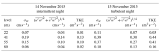
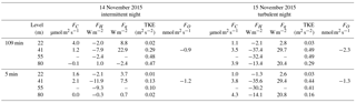
Table 1Five-minute turbulence statistics averaged for each night analyzed in Sect. 3.
The turbulence structure above forested canopies has been an important subject of research over the past decades. Such knowledge is essential to answer relevant scientific questions such as the quantification of the exchange of scalars between forested ecosystems and the atmosphere. Some of the precursor studies in this field have been performed in the Amazon region during projects such as the Atmospheric Boundary-Layer Experiment (ABLE 2A and 2B; Fan et al., 1990; Fitzjarrald et al., 1988; Garstang et al., 1990). Subsequent projects in this region that kept the focus on this subject include the Anglo-Brazilian Amazonian Climate Observation Study (ABRACOS; Grace et al., 1995; Kruijt et al., 2000; Malhi et al., 1998), the Large-Scale Biosphere-Atmosphere Experiment in Amazonia (LBA; Araújo et al., 2002; Miller et al., 2004; Saleska et al., 2003), Observations and Modeling of the Green Ocean Amazon (GOAmazon; Fuentes et al., 2016; Santos et al., 2016) and, most recently, the Amazon Tall Tower Observatory (ATTO; Andreae et al., 2015; Zahn et al., 2016).
Ultimately, one of the most relevant questions that these projects aimed to answer is the role of the Amazon rain forest as either a net sink or source of CO2 to the atmosphere. Results diverge greatly among the studies, from a net sink of 5.9 found by Grace et al. (1995) to a net source of 1.3 found by Saleska et al. (2003). Although some of this variability may be accepted as genuine, caused by site or interannual differences, it is now well established that methodological problems affected the estimates that found enhanced carbon uptake. Most of these issues regard the treatment of nocturnal data as a consequence of the complex nature of the atmospheric flow during the night under stable conditions. In particular, during very stable nights, turbulent mixing is reduced and constrained to small temporal scales (Acevedo et al., 2014; Vickers and Mahrt, 2006). The exchange of properties such as CO2 from the forest to the atmosphere may occur mostly through nonturbulent motion, such as drainage flows (Aubinet et al., 2003; Feigenwinter et al., 2004; Staebler and Fitzjarrald, 2004; Tóta et al., 2008) or by transport on temporal scales longer than those that characterize the turbulent flow (Santos et al., 2016).
The motion with temporal fluctuations longer than turbulence but smaller than those produced by mesoscale systems has been referred to as “submeso” by Mahrt (2009), and it has become an important subject of micrometeorological research since then. Typically, these nonturbulent fluctuations may be larger in magnitude than their turbulent counterpart, and they may introduce fluxes that are larger as well. On the other hand, these fluxes are not driven by local gradients, so that they are also much more variable than the turbulent fluxes and of either sign, in such a way that their overall contribution frequently averages out over longer periods (Vickers and Mahrt, 2003). Nevertheless, their contribution may be important for closing the budgets over smaller time periods (Acevedo and Mahrt, 2010; Kidston et al., 2010).
Many studies on turbulence above and within forested canopies have presented an analysis of the spectral distribution of the turbulence velocity components and of their vertical variation with respect to the canopy top (Baldocchi and Meyers, 1988; Blanken et al., 1998; Dupont and Patton, 2012). In general, these studies focused on the timescale of the turbulent exchange and how it depends on factors such as distance from canopy top and atmospheric stability. Equivalent analyses focusing on scalar flux cospectra have not been presented as often. Sakai et al. (2001) and Finnigan et al. (2003) used cospectral similarity to conclude that low-frequency contribution could account for missing energy and CO2 fluxes in their respective budgets, but neither study addressed how the cospectra varied across the canopy. Other studies (Campos et al., 2009; Fares et al., 2014) looked at scalar flux cospectra with the specific purpose of identifying the proper temporal scale for turbulent flux determination. Santos et al. (2016) found that horizontal turbulent kinetic energy (TKE) spectra are bimodal above an Amazonian rain forest canopy, with the peak on short timescales being related to turbulence and the peak on longer timescales being associated with nonturbulent, submeso fluctuations. Within the canopy, on the other hand, only the peak on longer timescales is preserved, indicating that nonturbulent fluctuations above the canopy propagate downward more efficiently than the turbulent ones. They also found that sensible heat flux cospectra within the canopy peaked on longer timescales, again similar to those of the nonturbulent maxima of horizontal TKE above the canopy. This result indicates that the exchange of scalars within the canopy at night may occur on longer timescales than those traditionally used in the eddy covariance approach. Under very stable conditions, such long scales may also contribute to the total exchange between the canopy and the atmosphere. Santos et al. (2016), however, did not include the analysis of CO2 or latent heat fluxes and reactive trace gases like O3, so that the question of whether these quantities are affected by similar processes remains open.
A comparison of scalar flux cospectra within and above a forested canopy, aimed specifically at addressing the contribution of nonturbulent flow to the total fluxes at the different heights, has not been presented previously. The present study aims at addressing this issue and to evaluate how these exchange processes affect the scalar profiles that are routinely measured at ATTO.
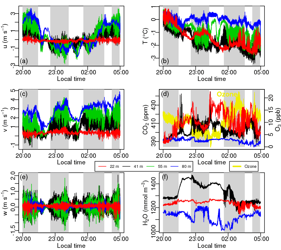
Figure 2Same as Fig. 1 but for the intermittent night. Shaded areas indicate intermittent turbulence bursts.
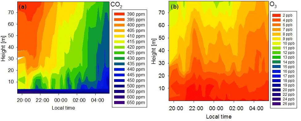
Figure 3Concentrations of CO2 (a) and O3 (b) as a function of time and height for the turbulent night.
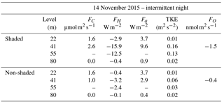
Table 2Five-minute TKE and fluxes averaged for shaded and non-shaded areas in the intermittent night (see Fig. 2).
2.1 Experimental site
The dataset was collected during the Intensive Operating Period (ATTO-IOP1) in October/November 2015 at Reserva de Desenvolvimento Sustentável Uatumã (Uatumã Sustainable Development Reserve – USDR), in the Amazon region. The site is located on a plateau at 120 , approximately 150 km northeast of Manaus and 12 km northeast of the Uatumã River. The average height of the highest trees near the tower is 37 m. Further information regarding terrain, soil, and vegetation can be found at Andreae et al. (2015).
Micrometeorological observations were carried out on an 80 m walk-up tower with rectangular cross sections at five different levels: 14, 22, 41, 55, and 80 m above the ground. The first two levels are within the forest canopy, while the three others are above it. Fast-response wind measurements were performed at all levels (CSAT3, Campbell Scientific Inc., at 14, 41, and 55 m; IRGASON, Campbell Scientific Inc., at 22 m; and Windmaster, Gill Instruments Limited, at 80 m). Temperature has been measured by a profile of thermohygrometers and by the sonic anemometers, as well. The thermohygrometers have been intercompared, while each sonic temperature has been compared to the closest thermohygrometer. Scalar concentrations of CO2 and water vapor were measured at 22 m (IRGASON, Campbell Scientific Inc.), 41, and 80 m (LI-7500A, LI-COR Inc.). The diurnal cycle of the H2O mixing ratios at 41 m was erroneous for unidentified reasons. The short-term (up to 20 min) variations were correct, but the longer trend agreed neither with the other open path instruments at 22 and 80 m nor with a nearby psychrometer (Frankenberger type, Theodor Friedrichs GmbH, Germany) or with the profile measurements (see below). Therefore, the water vapor mixing ratios at that level haven been corrected by separating the short-term fluctuations from the trend by applying a running mean with a window size of 5 min and adding this high-frequency contribution to the running mean (window size 5 min) of the nearby psychrometer. Scalar concentrations of ozone were measured at 41 m with chemiluminescence O3 sondes (Enviscope, Germany). In front of the fast O3 instrument there was a 5 m long (7.52 mm inner diameter) Teflon tubing with a Teflon inlet filter (47 mm diameter, 5 µm pore size). The flows varied due to filter clogging. After a filter change the flows were 21 and 23.5 L min−1, respectively, whereas before the filter change they were 16 and 14 L min−1, respectively. The resulting lag times were 0.6–0.95 s, and the Reynolds numbers in the tubing were 2400 to 4000 at 35 ∘C. On the days considered for the case studies (14 and 15 November), the flow was about 16 L min−1, and the residence time was therefore 0.8 s. All the data were collected at a rate of 10 Hz. As the signal of the fast O3 sondes has considerable drift, it was calibrated to a slow O3 analyzer (TEI 49i, Thermo Scientific) as described by Zhu et al. (2015). The CO2 profiles were measured sequentially by CO2∕H2O analyzers (LI-7000, LI-COR Inc.) connected to heated inlets at eight heights (0.05, 0.5, 4.0, 12.0, 24.0, 38.3, 53.0, and 79.3 m). During the case study nights (14 and 15 November), only the LI-7000 behind the Nafion® dryer was running, and therefore the water vapor values could not be used. The O3 profiles were also measured using the same inlet system with an ozone analyzer (TEI 49i, Thermo Scientific). Ambient air was continuously drawn from the inlets through nontransparent PTFE tubing () to a valve block, which switched between the different inlet levels, so that one intake height was purged by the sample pump (PTFE coated), while all the others were purged by the bypass pump. A time interval of 1 min was necessary for getting a constant and reliable signal for each concentration level: a complete cycle took 8 × 2 = 16 min, providing two measurements per level. Three 16 min measurement cycles plus one shorter 12 min cycle were performed every hour. During that last cycle, a small compromise was made to fit four cycles into the hour, and valve switches occurred every 90 s, thereby allowing for only one concentration measurement at each level. The ambient air inlets mounted on the tower were protected from rain entering the inlet line by polyethylene funnels and from insects by polyethylene nets. A PTFE filter (5 µm) was installed right after the inlet. The tubing was insulated with Styrofoam and heated. The internal temperature and pressure corrections of the LI-7000 were used, but to further minimize pressure effects, the air drawn from the inlets for analysis was sampled at the exit of the Teflon pump, so that the measurements were made close to ambient pressure for all measurement levels. The entire setup was comparable to the profile system employed by Mayer et al. (2011).
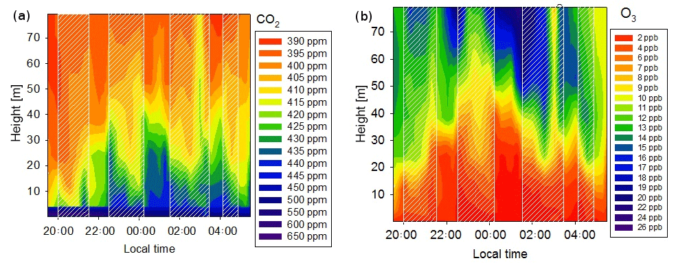

Figure 5Fluxes of sensible heat (a and b), CO2 (c and d), O3 (e and f), and latent heat (g and h) for the turbulent night (a, c, e, g) and for the intermittent night (b, d, f, h). Shaded areas indicate intermittent turbulence bursts as shown in Fig. 2.
Table 3TKE and fluxes averaged for each night analyzed in Sect. 3 using a time window of 5 and 109 min.
2.2 Data analysis
In the present study, 20 days of nocturnal data were analyzed, from 1 to 20 November 2015. To avoid sampling intense events associated with the transitional characteristics between daytime and nocturnal boundary layers, the evening period between the sunset and 20:00 local time (LT) was not considered for this analysis. For this reason, nocturnal periods were restricted to the time from 20:00 to 05:00 LT. Since the different levels of flow structures are analyzed simultaneously, only the data when all levels were available were used. The 14 m level frequently presented gaps and was not considered for this study. Therefore, the levels included are one inside the canopy (22 m), one just above canopy top (41 m), and two well above the canopy (55 and 80 m).
All the time series have been subject to quality control, which caused the removal of those series which showed multiple spikes or multiresolution spectra that displayed noise on the shortest timescales. For any case where a given series was discarded for a given variable, it has not been used for any of the variables. With these restrictions, 15 nights were kept for the final analysis. Ozone measurements started on 11 November 2015, so that only nine nights of ozone flux data were available.

Figure 6Average TKE spectra for the turbulent night (black solid lines) and the intermittent night (red dashed lines) for all levels, as indicated in each panel. In all panels, averages are calculated for each timescale.
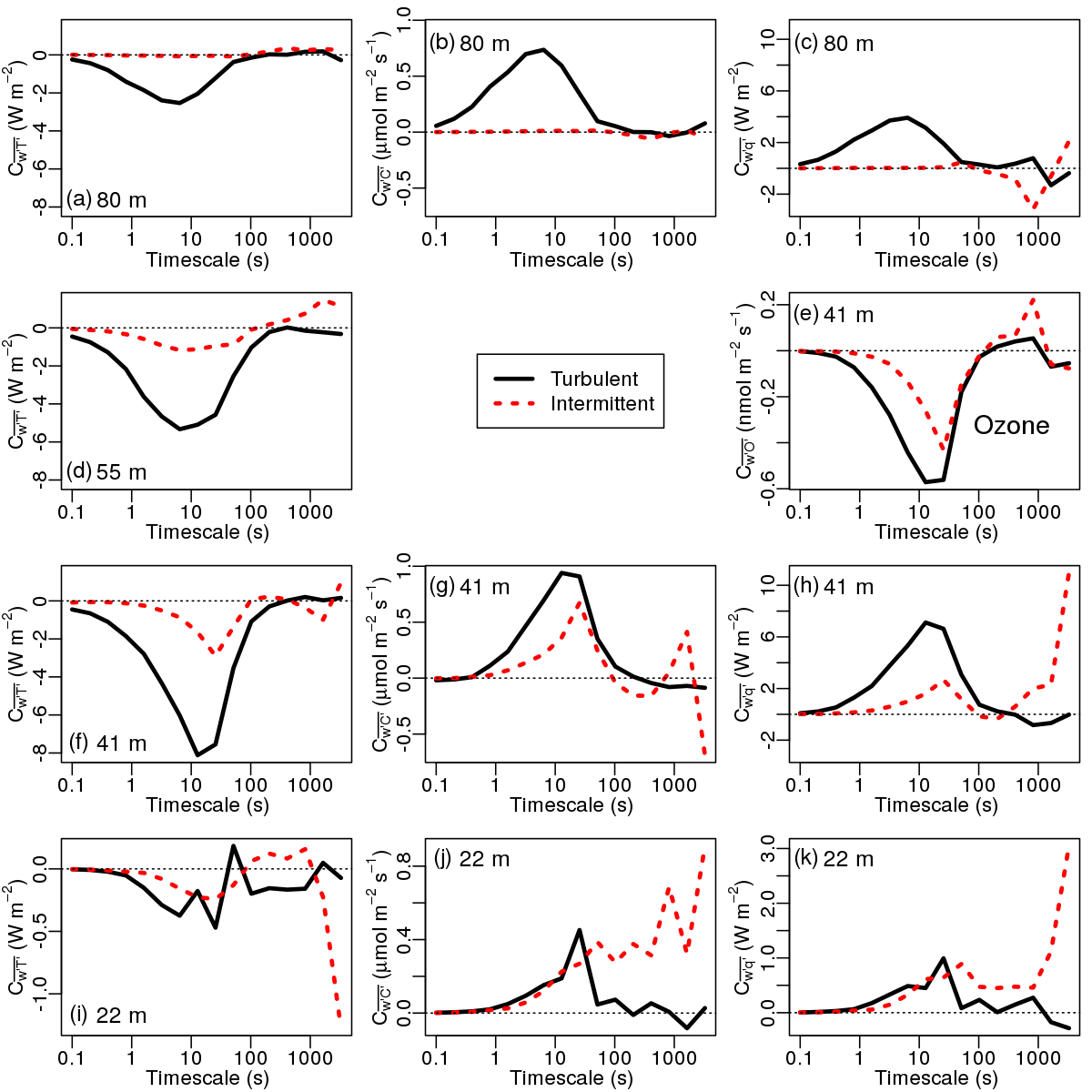
Figure 7Average cospectra of sensible heat (a, d, f, i), CO2 (b, g, j), O3 (e), and latent heat fluxes (c, h and k) for the turbulent night (black solid lines) and the intermittent night (red dashed lines) for all levels, as indicated in each panel. In all panels, averages are calculated for each timescale.
The data were analyzed using two different time windows: 5 and 109 min. The multiresolution decomposition (Howell and Mahrt, 1997; Vickers and Mahrt, 2003; Voronovich and Kiely, 2007) was applied to 109 min, which corresponds to groups of 216 data points. In contrast to the Fourier transform, which determines periodicity, this technique mainly extracts the width of the dominant turbulent events by locally decomposing the variances. For this reason, the multiresolution spectrum (S) and cospectrum (C) have the property that the integration up to a given timescale t is equal to the variance and covariance, respectively, for a t-long time series. Consequently, the multiresolution value for a given timescale captures the physical processes (and the flux) whose duration is smaller than that timescale.
The multiresolution decomposition was applied sequentially to the time series, starting at 20:00 LT, with an overlap of 30 min between the subsequent series, totaling 14 decompositions for each night. A total of 200 series was used in the study, considering all nights. Acevedo and Mahrt (2010) used the multiresolution decomposition to analyze vertical profiles of the nonturbulent component of sensible heat fluxes. They found that systematic and organized profiles, whose inclusion contributes to the closure of the nocturnal temperature budget near the surface, are only found when the double wind rotation (Tanner and Thurtell, 1969) is applied to each time series analyzed, separately. They claim that this is more suitable for such analysis than other coordinate rotation procedures, such as globally directionally dependent methods (Lee, 1998; Mahrt et al., 2000; Paw U et al., 2000) because “the measured vertical motion on times scales greater than 5 h may be sufficiently weak and unreliable that the elimination of larger-scale variations in vertical motion through coordinate rotation improves the calculation”. For these reasons, the double rotation was applied to each 109 min time series separately.
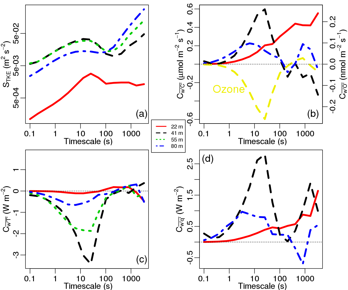
Figure 8Average spectra of TKE (a) and cospectra of CO2 and O3 (b), sensible heat (c), and latent heat (d) fluxes for the entire dataset. In all panels, averages are calculated for each timescale.
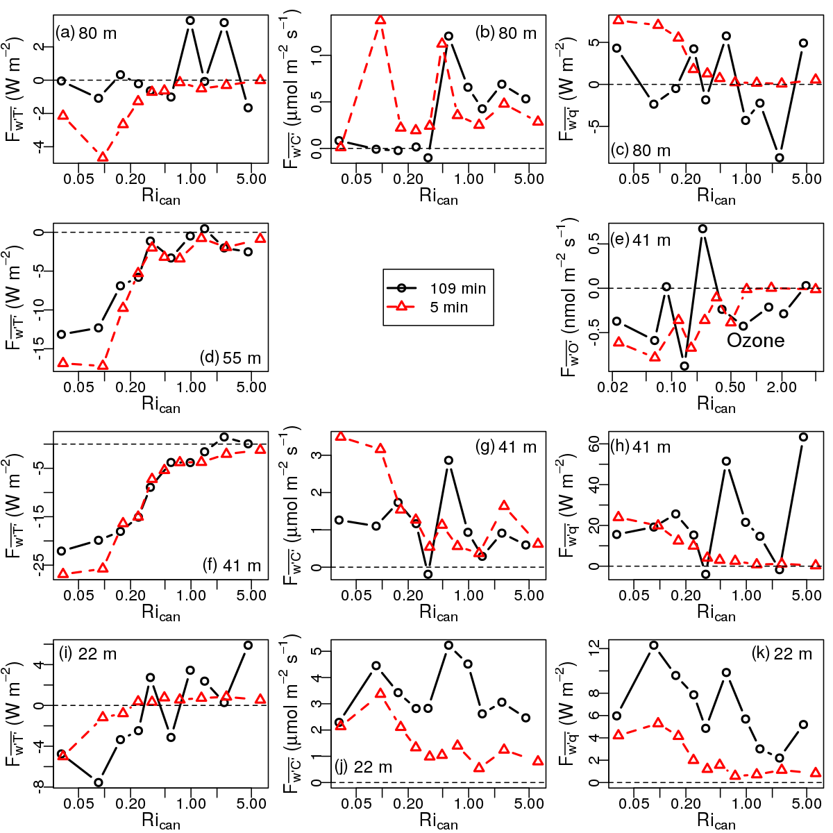
Figure 9The dependence of sensible heat (a, d, f, i), CO2 (b, g, j), O3 (e), and latent heat (c, h and k) fluxes on canopy Richardson number (Rican) for all levels, as indicated in each panel. Fluxes have been determined with 5 min (red lines, triangles) and 109 min (black lines, circles) time windows.
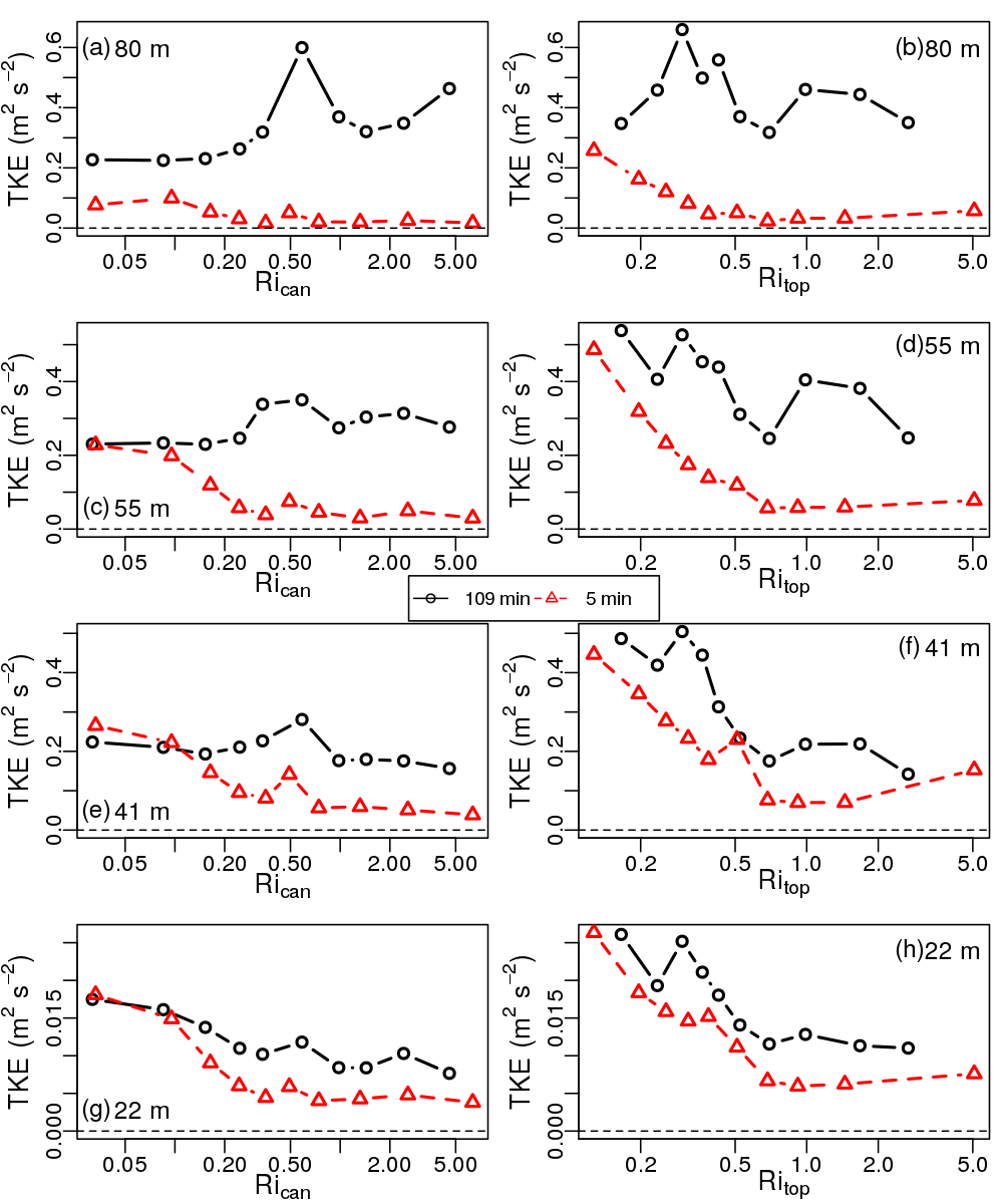
Figure 10The dependence of TKE on canopy Richardson number (Rican; a, c, e, g) and top Richardson number (Ritop; b, d, f, h) for all levels, as indicated in each panel, using 5 min (red lines, triangles) and 109 min (black lines, circles) time windows.

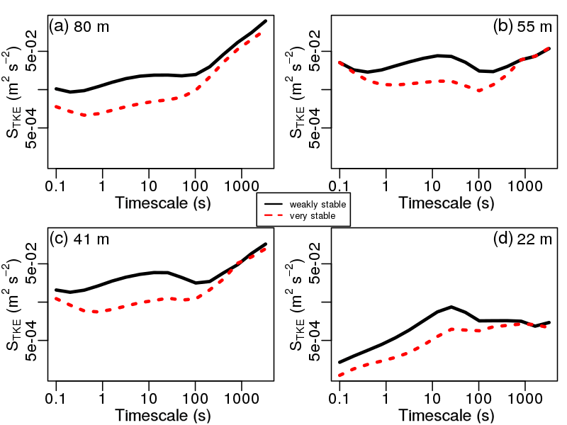
Figure 12Average TKE spectra for the weakly stable (black solid lines) and the very stable (red dashed lines) cases for all levels, as indicated in each panel. In all panels, averages are calculated for each timescale.
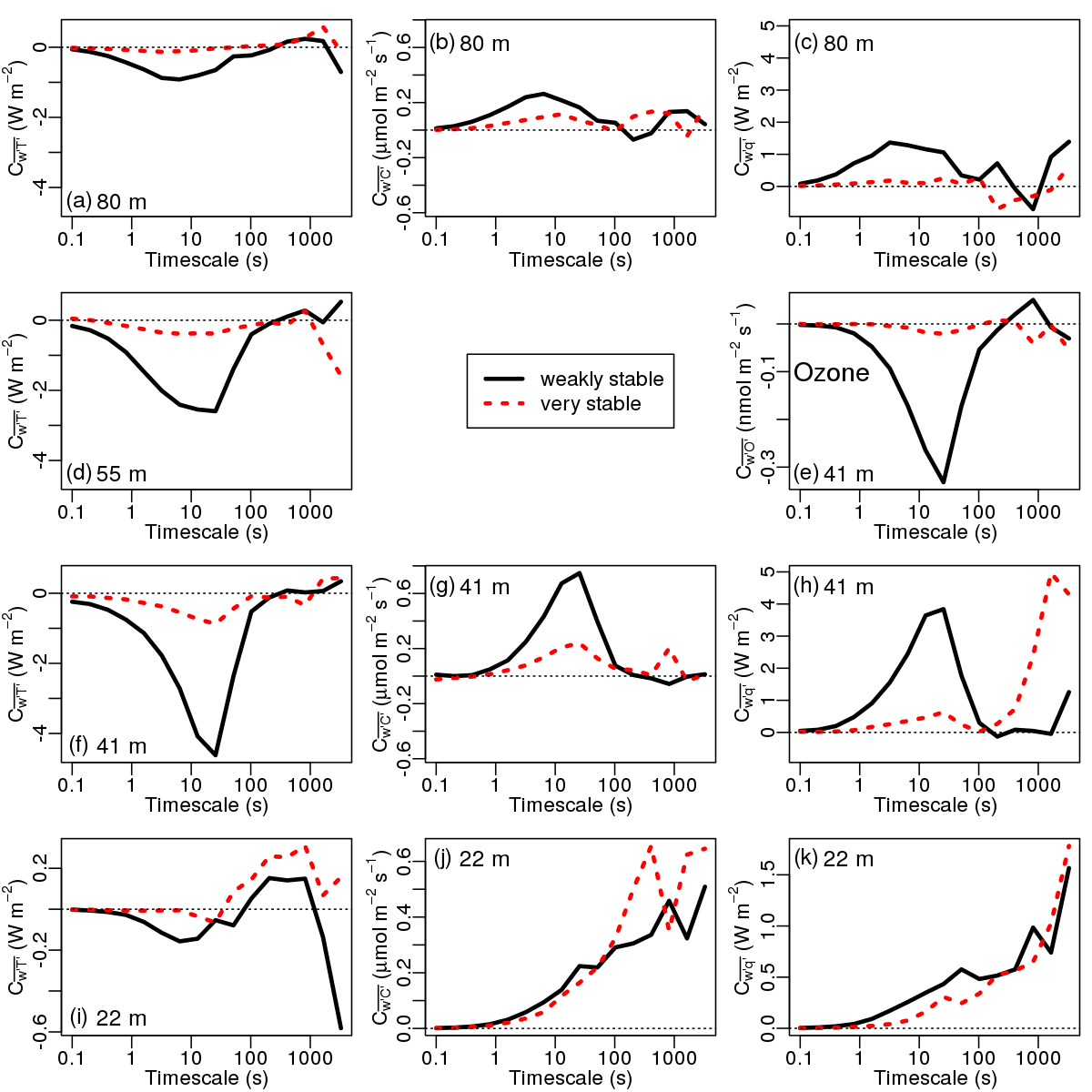
Figure 13Average cospectra of sensible heat (a, d, f, i), CO2 (b, g, j), O3 (e), and latent heat fluxes (c, h and k) for the weakly stable (black solid lines) and the very stable (red dashed lines) cases for all levels, as indicated in each panel. In all panels, averages are calculated for each timescale.
Variances and fluxes with a 109 min long time average were obtained from the integration of the respective multiresolution spectra and cospectra for each series separately and then averaged, if appropriate. Therefore, sensible and latent heat, CO2, and ozone fluxes are given by , , , and ; turbulent kinetic energy is and the SD of the vertical wind component is . Other variables, such as the Richardson number (Ri) and average horizontal wind speed (V), were calculated using the same time interval used in the multiresolution decomposition.
At night, it is expected that the temporal scales of turbulent transport are smaller. Campos et al. (2009) showed that the contribution of turbulence to the nocturnal fluxes above the canopy at another site in the Amazon forest occurs on temporal scales smaller than 200 s. The use of a 109 min long time window is necessary to determine the contribution of turbulent and nonturbulent motions to the fluxes. However, in order to attempt to reduce any contribution from nonturbulent transport, statistical moments, fluxes, and other variables were also calculated using a 5 min time window, as used by Dupont and Patton (2012). Quantities such as sensible heat , latent heat , CO2 , ozone fluxes, turbulent kinetic energy (TKE), the average horizontal wind speed (V), Richardson number (Ri), and σw were determined for both 5 and 109 min. The turbulent velocity scale, defined as , was calculated for 5 min time windows only. This study comprises a total of 1577 5 min windows.
The bulk Richardson number was used to quantify atmospheric stability. The choice of the bulk instead of the flux Richardson number for the analysis has two reasons: to avoid self-correlation (Baas et al., 2006; Hicks, 1978; Klipp and Mahrt, 2004) and to quantify better the stability in very stable conditions when fluxes are expected to approach 0. Similarly to usage in Bosveld et al. (1999), Mammarella et al. (2007), and Oliveira et al. (2013), a “within-canopy Richardson number” (Rican) and an “above-canopy Richardson number” (Ritop) (Santos et al., 2016) were defined as
and
where g is the gravitational acceleration, Θ is the average potential temperature in the layer, Δz is the height difference between the two levels, and θ and V are the mean potential temperature and average horizontal wind speed at each level, respectively.
The nocturnal flow at the site is characterized by the superposition of turbulent and nonturbulent fluctuations. In a fully turbulent night, such as 15 November 2015 (Fig. 1), there is a clear dominant wind direction at all levels. In this case, it is very rare that the horizontal wind components switch sign above the canopy. In contrast, during the intermittent night of 14 November 2015 (Fig. 2), there is no dominant wind direction at any level above the canopy, as both horizontal components switch sign many times throughout the night. Low-frequency fluctuations are superposed on the turbulent fluctuations, causing the mean wind direction to change quadrants frequently throughout the night. Such fluctuations have been recently attributed to submeso flow (Mahrt, 2009), while in the pollutant dispersion community similar phenomena are often referred to as meandering (Oettl et al., 2005). The most relevant difference between the two nights regards the magnitude of the turbulent mixing (Table 1). All relevant turbulence statistics are significantly larger on 15 November than on 14 November. The relative difference of the turbulence statistics between nights increases steadily in the vertical. As an example, TKE at 41 m is 3.4 times larger in the turbulent night than in the intermittent case, while at 80 m, TKE is 8.2 times larger in the turbulent night. Similar increases occur for the corresponding ratios of σw and between the two nights.
Another interesting characteristic that indicates a contrast between the two nights shown in Fig. 1 and Fig. 2 regards the degree of vertical coupling across the levels, a phenomenon that has been observed by van Gorsel et al. (2011), Oliveira et al. (2013), and Jocher et al. (2017). In the turbulent night, temperatures were always similar between the levels of 41 and 55 m, while at 80 m, it was slightly warmer, but with the same cooling tendency throughout the period. CO2 was correspondingly similar between 22 and 41 m, with the same tendencies and slightly lower values at 80 m. Although the mean trend is similar at 22 and 41 m, substantial, short time deviations towards higher CO2 values were observed at 22 m (Fig. 1d). This is in line with the higher variability in CO2 values in the lower canopy, as can be seen from the profiles (Fig. 3a). This higher variability and stronger gradient (in both CO2 and O3) in the lower canopy point to a decoupling of the sub-canopy even in the turbulent night. As the 22 m level is within the maximum of the leaf area index (LAI) (∼ 24 m), which separates the upper canopy from the lower canopy, it will be influenced by both regimes. The gradients between 24 and 38 m are always positive for O3 and negative for CO2. This can be related to the reactivity of O3 as it reacts with compounds emitted from the soil (mainly NO) and plants (alkenes) and is not only taken up by stomata but is also deposited to leaf surfaces in considerable amounts, especially under humid conditions (Fuentes and Gillespie, 1992; Rummel et al., 2007). At night, CO2 is emitted by soils and plants due to respiration, causing a negative gradient.
All quantities showed much larger variation across the levels in the intermittent night (Fig. 2). Furthermore, sporadic events of coupling occurred during bursts of intermittent turbulence (Fig. 2, shaded areas). It has been assumed that the turbulent bursts occurred whenever σw > 0.15 ms−1. During these events of coupling, the gradients of temperature and CO2 concentration became sporadically smaller across the vertical, except for the 80 m level, indicating that the coupling induced by the events extended over a layer shallower than 80 m. In general, the temporal evolution of all scalars shows a monotonic increase (in CO2) or decrease (in temperature and O3) throughout the turbulent night at all levels (Fig. 1). In the intermittent night, on the other hand, large increases and decreases in all scalars occur in small periods of time at all levels, except at 80 m. As CO2 has a clear source at the ground and O3 has a clear sink at the ground, one can identify from the profiles whether air is coming from aloft or from below (Fig. 4). Air from above is rich in O3 and lower in CO2, whereas air from below is rich in CO2 but depleted in O3. From this perspective, in the first event air is mixed down from aloft, while in the second event air is mixed both upward and downward from the canopy top. In the third event, air is first mixed down and finally there is a burst of air going upwards from the canopy. At 80 m, temperature (Fig. 2b) and CO2 (Fig. 2d) show much smaller fluctuations than at the other levels. This is further evidence that the stable boundary layer (SBL) thickness is shallower during the intermittent night, such that the canopy exchange fluxes do not affect the state of the atmosphere at 80 m. This fact contrasts strongly with the steady trends in both scalars at 80 m during the turbulent night (Fig. 1b and Fig. 1d), which indicates that in this case, this level is fully coupled through turbulence to the canopy top. While in the turbulent nighttime, scalar fluxes did not vary substantially throughout the period (Fig. 5a, c, e, and g), the most intense turbulent fluxes of sensible heat (Fig. 5b), CO2 (Fig. 5d), O3 (Fig. 5f), and latent heat (Fig. 5h) during the intermittent night occurred during these coupling periods (Table 2).
Previous studies have reported that nonturbulent modes of the flow only become relevant when turbulence is weak (Acevedo et al., 2014), a likely consequence of the diffusive nature of turbulence destroying the nonturbulent temporal and spatial variability in the atmospheric variables. This relationship between the turbulent and nonturbulent modes of the flow is illustrated by the TKE spectrum during both nights (Fig. 6). In the turbulent case, most of the energy is associated with turbulence, so that the most energetic timescale is near 10 s at all levels, except for 80 m (Fig. 6a). At this level, the longest timescales are the most energetic, but the 10 s turbulent maximum and a cospectral gap (near 100 s) are still evident. In contrast, in the intermittent night of 14 November, at all levels most energy prevails on the longest timescales provided by the decomposition method. This energy is associated with the low-frequency fluctuations responsible for the variability in the wind direction visible in Fig. 2a and Fig. 2c. These spectra confirm that when fully turbulent conditions prevail, the energy of the nonturbulent, low-frequency modes of the flow is reduced considerably. The cospectra of the fluxes of sensible heat (Fig. 7a, d, f, and i), CO2 (Fig. 7b, g, and j), O3 (Fig. 7e), and latent heat (Fig. 7c, h, and k) confirm the enhanced turbulent exchange of all quantities in the turbulent night compared to the intermittent one. They also show that, consistently to what occurs with TKE, the nonturbulent exchange of these scalars is enhanced in the intermittent case. In particular, a significant low-frequency flux of CO2 occurs at 22 m in the intermittent night, such that the total flux at this level is larger during the intermittent night (4.0 µmol m2 s−1, Table 3) than during the turbulent one (1.1 µmol m2 s−1) when all scales of the motion that are captured by the decomposition window are considered. This is in line with the idea that nonturbulent motions better penetrate the canopy. The same occurs for latent heat, which shows a mean flux of 8.8 W m−2 in the intermittent night and of 2.8 W m−2 in the turbulent night when all scales are considered. Even for 5 min fluxes, the larger fluxes still occur in the intermittent night (1.7 vs. 1.0 µmol m2 s−1 in the turbulent night for CO2 and 3.8 vs. 2.5 W m−2 for latent heat), but the differences are smaller. These numbers show that the low-frequency contributions dominate the exchange of CO2 and moisture in the interior of the forest in the intermittent night. Santos et al. (2016) found that the dominant timescales of the vertical velocity fluctuations and sensible heat flux within an Amazonian rain forest canopy (at a different site) are shifted towards larger values than those above it. Our results support these findings, adding the information that the exchanges of CO2 and humidity within the canopy are also dominated by nonturbulent contribution at very stable nights. It is likely that the same process affects other scalars, such as O3, whose concentrations are perturbed by intermittent events as shown in Fig. 4b.
Another interesting contrast between the turbulent and intermittent nights can be seen for the sensible heat (Fig. 7a), CO2 (Fig. 7b), and latent heat (Fig. 7c) cospectra at 80 m, which show an almost total absence of turbulent fluxes (timescale smaller than 100 s) of these quantities at this height in the intermittent case. This result explains the reduced fluctuations in temperature (Fig. 2b) and CO2 (Fig. 2d) at 80 m in the intermittent night, adding evidence to the suggestion that the SBL may be rather shallow in that night, possibly such that the 80 m level is near its top. The large fluctuations in water vapor at 80 m (Fig. 2f) may be related to the enhanced low-frequency flux of this quantity during this night (Fig. 7c).
Figure 8 shows the spectra and cospectra of the turbulent fluctuations and fluxes averaged over the entire period of 15 nights. The distinction between turbulent and nonturbulent fluctuations across the vertical is evident in the averaged TKE spectra (Fig. 8a). On average, a timescale around 100 s separates the two types of fluctuations. This can be seen by the fact that STKE decreases with height above the canopy, following what typically happens to turbulent fluctuations in the stable boundary layer (Kruijt et al., 2000; Santos et al., 2016) only for timescales smaller than 100 s. For longer timescales, STKE increases with height. This result has been previously shown by Andreae et al. (2015) at the same tower but for a different period. The average cospectra of all scalars show the largest turbulent fluxes at 41 m, with a sharp maximum on a timescale around 30 s. Within the canopy, systematic positive fluxes of CO2 and latent heat happen on all timescales. The magnitude increases with increasing timescale. Therefore, this is an indication that the CO2 and humidity exchanges in the interior of the forest may be, to a large extent, caused by nonturbulent motion. This process will be further investigated later in this paper when the scale dependence of the fluxes is compared to the stability within and above the canopy. The average sensible heat cospectrum at 22 m is negative for timescales smaller than 50 s and positive for larger timescales. Santos et al. (2016) showed that sensible heat fluxes near the forest floor are positive for all timescales, while they are negative for all timescales at the canopy top. At intermediate heights, they tend to be like those shown in Fig. 8c. These authors also showed that the height within the canopy where the total sensible heat flux switches sign from upward at lower levels to downward at higher levels is stability dependent, increasing as it becomes more stable.
The comparison of the fluxes determined with 5 min and 109 min time windows and their stability dependence for the entire period of 15 nights provides interesting information on the scalar exchange processes within and above the canopy. Sensible heat flux at 22 m (Fig. 9i) switches sign at intermediate stability for both 5 min and 109 min averaging periods. This is in agreement with the result obtained by Santos et al. (2016) that the height where the sensible heat flux switches sign is stability dependent. In the present case, the critical value at which the 5 min sensible heat flux at 22 m switches sign is 0.25. At the same height, CO2 (Fig. 9j) and latent heat (Fig. 9k) fluxes are similar with both averaging times at near-neutral conditions but become appreciably larger with 109 min windows than with 5 min windows as conditions become more stable. This result confirms the idea that the CO2 and humidity exchange within the canopy at very stable conditions are dominated by processes with long timescales. At 41 m (Fig. 9e–h), 55 m (Fig. 9d), and 80 m (Fig. 9a–c), the 109 min fluxes of scalars are more erratic, sometimes with no clear dependence on Rican. The 5 min fluxes, on the other hand, show a tendency to decrease in magnitude with stability at all heights above the canopy. The 5 min TKE decreases with stability at all levels (Fig. 10), but at 80 m it becomes near 0 for Rican>0.2. This is the same range of stability for which the 5 min fluxes of heat and CO2 are virtually suppressed, indicating that in these very stable conditions the stable boundary layer thickness may be close to 80 m or shallower. When the same quantities are compared to Ritop (Fig. 11), the most significant difference is that the 109 min fluxes at 41 m (Fig. 11e–h, black lines) and 55 m (Fig. 11d, black line) show a more systematic dependence on stability. This result indicates that the low-frequency exchange at the canopy top and above is controlled by the stability over a large distance above the forest.
The 0.25-Rican threshold, over which the 22 m turbulent sensible heat flux switches sign, is used to classify each series as weakly stable (Rican≤0.25) or very stable (Rican>0.25). The average spectra for each of these classes are shown in Fig. 12. At all levels, the low-frequency TKE is almost independent of stability, as for timescales larger than 100 s the TKE spectra of the very stable series approach those of the weakly stable ones. For smaller timescales, on the other hand, a significant distinction prevails, with TKE being many times larger under weakly stable conditions than during very stable conditions. The turbulent portions of the scalar fluxes above the canopy (41 m and above) respond accordingly, always being much larger in magnitude in the weakly stable cases (Fig. 13).
At 22 m, the criterion for classifying the time series ensures that the sensible heat flux on small timescales must be negative under the weakly stable conditions and positive under the very stable ones. This is shown in Fig. 13i, but it is remarkable that even in the weakly stable cases, there is a range of timescales for which the sensible heat flux within the canopy is upward. This range is also observed (however broader) in the very stable class, although in this case the negative maximum associated with turbulent exchange is absent. This result shows that low-frequency exchange of heat within the canopy is consistently upward, regardless of stability. Therefore, the main control exerted by stability regards the depth within the canopy where the downward turbulent heat flux penetrates (Santos et al., 2016). The total 22 m fluxes of CO2 (Fig. 13j) are larger in the very stable class than in the weakly stable one, which is mainly caused by the contribution of timescales larger than 100 s, corroborating the results from the case studies (Sect. 3). For latent heat (Fig. 13k), the total flux is slightly larger in the weakly stable cases, and this result is mainly caused by the contributions of fluxes with timescales smaller than 100 s.
The main novelty of the present study has been a detailed analysis of different scalar fluxes and their timescales within and above a rain forest canopy at night. The data was collected at the ATTO and included fluxes of CO2, O3, and latent and sensible heat. The most relevant findings include the following.
-
Within the canopy, fluxes of CO2 and latent heat are dominated by processes with long timescales. Given that such low-frequency exchange tends to be enhanced in very stable conditions, the total scalar flux within the canopy may be larger in very stable nights than in weakly stable ones.
-
In very stable nights, turbulent fluxes are effectively suppressed at 80 m, indicating that a very shallow SBL may exist in these situations.
-
Intermittent turbulence may produce very large fluxes and affect concentrations of CO2 and O3 from near the SBL top down to the middle of the canopy.
Although low-frequency contributions to the fluxes are enhanced during very stable nights, their inclusion into the scalar budgets is not enough to bring the nocturnal fluxes in the very stable nights close to those observed during fully turbulent conditions. Processes such as drainage flows or local storage may account for the differences.
Turbulent exchange is always important just above the canopy (41 m level, in this case), but, in very stable nights, the nonturbulent contribution also has to be considered. Campos et al. (2009) found the low-frequency contribution of CO2 fluxes above a similar Amazonian canopy to be seasonally dependent, a result that could not be examined with the present data set.
A fully instrumented 320 m tower is expected to start operating continually in the near future at the ATTO site. It will allow addressing questions such as the seasonality of the exchange on different scales, as well as the thickness of the SBL and the nature of the scalar exchange within and above the canopy in much more detail. In this sense, the results of the present study will provide important guidelines for future investigations.
All data used in this study are kept in the ATTO Databases at Instituto de Pesquisas da Amazônia and Max Planck Institut für Chemie. The overall project description can be found at http://www.mpic.de/en/research/collaborative-projects/atto.html. Data access can be requested from the coauthors responsible for maintaining the dataset: Matthias Sörgel (m.soergel@mpic.de) and Alessandro Araújo (alessandro.araujo@gmail.com).
The authors declare that they have no conflict of interest.
This article is part of the special issue “Amazon Tall Tower Observatory (ATTO) Special Issue”. It is not associated with a conference.
For the operation of the ATTO site, we acknowledge the support by the German Federal Ministry of Education and Research
(BMBF contract 01LB1001A) and the Brazilian Ministério da Ciência, Tecnologia e Inovação (MCTI/FINEP contract
01.11.01248.00) as well as the Amazon State University (UEA), FAPEAM, LBA/INPA and SDS/CEUC/RDS-Uatumã. This work, in
particular, was supported by the Max Planck Society (MPG), the Instituto Nacional de Pesquisas da Amazônia (INPA), and the
Conselho Nacional de Desenvolvimento Científico e Tecnológico (CNPq).
Edited by: Gilberto Fisch
Reviewed by: two anonymous referees
Acevedo, O. C. and Mahrt, L.: Systematic vertical variation of mesoscale fluxes in the nocturnal boundary layer, Bound.-Lay. Meteorol., 135, 19–30, 2010. a, b
Acevedo, O. C., Costa, F. D., Oliveira, P. E. S., Puhales, F. S., Degrazia, G. A., and Roberti, D. R.: The influence of submeso processes on stable boundary layer similarity relationships, J. Atmos. Sci., 71, 207–225, https://doi.org/10.1175/JAS-D-13-0131.1, 2014. a, b
Andreae, M. O., Acevedo, O. C., Araùjo, A., Artaxo, P., Barbosa, C. G. G., Barbosa, H. M. J., Brito, J., Carbone, S., Chi, X., Cintra, B. B. L., da Silva, N. F., Dias, N. L., Dias-Júnior, C. Q., Ditas, F., Ditz, R., Godoi, A. F. L., Godoi, R. H. M., Heimann, M., Hoffmann, T., Kesselmeier, J., Könemann, T., Krüger, M. L., Lavric, J. V., Manzi, A. O., Lopes, A. P., Martins, D. L., Mikhailov, E. F., Moran-Zuloaga, D., Nelson, B. W., Nölscher, A. C., Santos Nogueira, D., Piedade, M. T. F., Pöhlker, C., Pöschl, U., Quesada, C. A., Rizzo, L. V., Ro, C.-U., Ruckteschler, N., Sá, L. D. A., de Oliveira Sá, M., Sales, C. B., dos Santos, R. M. N., Saturno, J., Schöngart, J., Sörgel, M., de Souza, C. M., de Souza, R. A. F., Su, H., Targhetta, N., Tóta, J., Trebs, I., Trumbore, S., van Eijck, A., Walter, D., Wang, Z., Weber, B., Williams, J., Winderlich, J., Wittmann, F., Wolff, S., and Yáñez-Serrano, A. M.: The Amazon Tall Tower Observatory (ATTO): overview of pilot measurements on ecosystem ecology, meteorology, trace gases, and aerosols, Atmos. Chem. Phys., 15, 10723–10776, https://doi.org/10.5194/acp-15-10723-2015, 2015. a, b, c
Araújo, A. C., Nobre, A. D., Kruijt, B., Elbers, J. A., Dallarosa, R., Stefani, P., von Randow, C., Manzi, A. O., Culf, A. D., Gash, J. H. C., Valentini, R., and Kabat, P.: Comparative measurements of carbon dioxide fluxes from two nearby towers in a central Amazonian rainforest: the Manaus LBA site, J. Geophys. Res.-Atmos, Finnig107, LBA 58-1–LBA 58-20, https://doi.org/10.1029/2001JD000676, 8090, 2002. a
Aubinet, M., Heinesch, B., and Yernaux, M.: Horizontal and vertical CO2 advection in a sloping forest, Bound.-Lay. Meteorol., 108, 397–417, https://doi.org/10.1023/A:1024168428135, 2003. a
Baas, P., Steeneveld, G. J., van de Wiel, B. J. H., and Holtslag, A. A. M.: Exploring self-correlation in flux-gradient relationships for stably stratified conditions, J. Atmos. Sci., 63, 3045–3054, https://doi.org/10.1175/JAS3778.1, 2006. a
Baldocchi, D. D. and Meyers, T. P.: A spectral and lag correlation analysis of turbulence in a deciduous forest canopy, Bound.-Lay. Meteorol., 45, 31–58, https://doi.org/10.1007/BF00120814, 1988. a
Blanken, P. D., Black, T. A., Neumann, H. H., Hartog, G. D., Yang, P. C., Nesic, Z., Staebler, R., Chen, W., and Novak, M. D.: Turbulent flux measurements above and below the overstory of a boreal aspen forest, Bound.-Lay. Meteorol., 89, 109–140, https://doi.org/10.1023/A:1001557022310, 1998. a
Bosveld, F. C., Holtslag, A. A. M., and Van den Hurk, B. J. J. M.: Nighttime convection in the interior of a dense Douglas fir forest, Bound.-Lay. Meteorol., 93, 171–195, https://doi.org/10.1023/A:1002039610790, 1999. a
Campos, J. G., Acevedo, O. C., Tota, J., and Manzi, A. O.: On the temporal scale of the turbulent exchange of carbon dioxide and energy above a tropical rain forest in Amazonia, J. Geophys. Res., 114, D08124, https://doi.org/10.1029/2008JD011240, 2009. a, b, c
Dupont, S. and Patton, E. G.: Influence of stability and seasonal canopy changes on micrometeorology within and above an orchard canopy: the {CHATS} experiment, Agr. Forest Meteorol., 157, 11–29, https://doi.org/10.1016/j.agrformet.2012.01.011, 2012. a, b
Fan, S.-M., Wofsy, S. C., Bakwin, P. S., Jacob, D. J., and Fitzjarrald, D. R.: Atmosphere-biosphere exchange of CO2 and O3 in the central Amazon forest, J. Geophys. Res.-Atmos., 95, 16851–16864, https://doi.org/10.1029/JD095iD10p16851, 1990. a
Fares, S., Savi, F., Muller, J., Matteucci, G., and Paoletti, E.: Simultaneous measurements of above and below canopy ozone fluxes help partitioning ozone deposition between its various sinks in a Mediterranean oak forest, Agr. Forest Meteorol., 198–199, 181–191, https://doi.org/10.1016/j.agrformet.2014.08.014, 2014. a
Feigenwinter, C., Bernhofer, C., and Vogt, R.: The influence of advection on the short term CO2 budget in and above a forest canopy, Bound.-Lay. Meteorol., 113, 201–224, 2004. a
Finnigan, J. J., Clement, R., Malhi, Y., Leuning, R., and Cleugh, H.: A re-evaluation of long-term flux measurement techniques Part I: Averaging and coordinate rotation, Bound.-Lay. Meteorol., 107, 1–48, https://doi.org/10.1023/A:1021554900225, 2003. a
Fitzjarrald, D. R., Stormwind, B. L., Fisch, G., and Cabral, O. M. R.: Turbulent transport observed just above the Amazon forest, J. Geophys. Res.-Atmos., 93, 1551–1563, https://doi.org/10.1029/JD093iD02p01551, 1988. a
Fuentes, J. D. and Gillespie, T. J.: A gas exchange system to study the effects of leaf surface wetness on the deposition of ozone, Atmos. Environ. A-Gen., 26, 1165–1173, https://doi.org/10.1016/0960-1686(92)90048-P, 1992. a
Fuentes, J. D., Chamecki, M., dos Santos, R. M. N., Randow, C. V., Stoy, P. C., Katul, G., Fitzjarrald, D., Manzi, A., Gerken, T., Trowbridge, A., Freire, L. S., Ruiz-Plancarte, J., Maia, J. M. F., Tóta, J., Dias, N., Fisch, G., Schumacher, C., Acevedo, O., Mercer, J. R., and Yáñez-Serrano, A. M. Y.: Linking meteorology, turbulence, and air chemistry in the Amazon rain forest, B. Am. Meteorol. Soc., 97, 2329–2342, https://doi.org/10.1175/BAMS-D-15-00152.1, 2016. a
Garstang, M., Greco, S., Scala, J., Swap, R., Ulanski, S., Fitzjarrald, D., Martin, D., Browell, E., Shipman, M., Connors, V., Harriss, R., and Talbot, R.: The Amazon Boundary-Layer Experiment (ABLE 2B): a meteorological perspective, B. Am. Meteorol. Soc., 71, 19–32, https://doi.org/10.1175/1520-0477(1990)071<0019:TABLEA>2.0.CO;2, 1990. a
Grace, J., Lloyd, J., McIntyre, J., Miranda, A. C., Meir, P., Miranda, H. S., Nobre, C., Moncrieff, J., Massheder, J., Malhi, Y., Wright, I., and Gash, J.: Carbon dioxide uptake by an undisturbed tropical rain forest in southwest Amazonia, 1992 to 1993, Science, 270, 778–780, https://doi.org/10.1126/science.270.5237.778, 1995. a, b
Hicks, B. B.: Some limitations of dimensional analysis and power laws, Bound.-Lay. Meteorol., 14, 567–569, https://doi.org/10.1007/BF00121895, 1978. a
Howell, J. F. and Mahrt, L.: Multiresolution flux decomposition, Bound.-Lay. Meteorol., 83, 117–137, https://doi.org/10.1023/A:1000210427798, 1997. a
Jocher, G., Löfvenius, M. O., Simon, G. D., Hörnlund, T., Linder, S., Lundmark, T., Marshall, J., Nilsson, M. B., Näsholm, T., Tarvainen, L., Öquist, M., and Peichl, M.: Apparent winter CO2 uptake by a boreal forest due to decoupling, Agr. Forest Meteorol., 232, 23–34, https://doi.org/10.1016/j.agrformet.2016.08.002, 2017. a
Kidston, J., Brümmer, C., Black, T. A., Morgenstern, K., Nesic, Z., McCaughey, J. H., and Barr, A. G.: Energy balance closure using eddy covariance above two different land surfaces and implications for CO2 flux measurements, Bound.-Lay. Meteorol., 136, 193–218, https://doi.org/10.1007/s10546-010-9507-y, 2010. a
Klipp, C. L. and Mahrt, L.: Flux-gradient relationship, self-correlation and intermittency in the stable boundary layer, Q. J. Roy. Meteor. Soc., 130, 2087–2103, https://doi.org/10.1256/qj.03.161, 2004. a
Kruijt, B., Malhi, Y., Lloyd, J., Nobre, A. D., Miranda, A. C., Pereira, M. G. P., Culf, A., and Grace, J.: Turbulence statistics above and within two Amazon rain forests canopies, Bound.-Lay. Meteorol., 94, 297–331, https://doi.org/10.1023/A:1002401829007, 2000. a, b
Lee, X.: On micrometeorological observations of surface-air exchange over tall vegetation, Agr. Forest Meteorol., 91, 39–49, https://doi.org/10.1016/S0168-1923(98)00071-9, 1998. a
Mahrt, L.: Characteristics of submeso winds in the stable boundary layer, Bound.-Lay. Meteorol., 130, 1–14, https://doi.org/10.1007/s10546-008-9336-4, 2009. a, b
Mahrt, L., Lee, X., Black, A., Neumann, H., and Staebler, R.: Nocturnal mixing in a forest subcanopy, Agr. Forest Meteorol., 101, 67–78, https://doi.org/10.1016/S0168-1923(99)00161-6, 2000. a
Malhi, Y., Nobre, A. D., Grace, J., Kruijt, B., Pereira, M. G. P., Culf, A., and Scott, S.: Carbon dioxide transfer over a central Amazonian rain forest, J. Geophys. Res.-Atmos., 103, 31593–31612, https://doi.org/10.1029/98JD02647, 1998. a
Mammarella, I., Kolari, P., Rinne, J., Keronen, P., Pumpanem, J., and Vesala, T.: Determining the contribution of vertical advection to the net ecosystem exchange at Hyytiälä forest, Tellus B, 59, 900–909, https://doi.org/10.1111/j.1600-0889.2007.00306.x, 2007. a
Mayer, J.-C., Bargsten, A., Rummel, U., Meixner, F., and Foken, T.: Distributed Modified Bowen Ratio Method for surface layer fluxes of reactive and non-reactive trace gases, Special Issue on Atmospheric Transport and Chemistry in Forest Ecosystems, Agr. Forest Meteorol., 151, 655–668, https://doi.org/10.1016/j.agrformet.2010.10.001, 2011. a
Miller, S. D., Goulden, M. L., Menton, M. C., da Rocha, H. R., de Freitas, H. C., Figueira, A. M. E. S., and Dias de Sousa, C. A.: Biometric and micrometeorological measurements of tropical forest carbon balance, Ecol. Appl., 14, 114–126, https://doi.org/10.1890/02-6005, 2004. a
Oettl, D., Goulart, A., Degrazia, G., and Anfossi, D.: A new hypothesis on meandering atmospheric flows in low wind speed conditions, Atmos. Environ., 39, 1739–1748, https://doi.org/10.1016/j.atmosenv.2004.11.034, 2005. a
Oliveira, P. E. S., Acevedo, O. C., de Moraes, O. L. L., Zimmermann, H. R., and Teichrieb, C. A.: Nocturnal intermittent coupling between the interior of a pine forest and the air above it, Bound.-Lay. Meteorol., 146, 45–64, https://doi.org/10.1007/s10546-012-9756-z, 2013. a, b
Paw U, K. T., Baldocchi, D. D., Meyers, T. P., and Wilson, K. B.: Correction of eddy-covariance measurements incorporating both advective effects and density fluxes, Bound.-Lay. Meteorol., 97, 487–511, https://doi.org/10.1023/A:1002786702909, 2000. a
Rummel, U., Ammann, C., Kirkman, G. A., Moura, M. A. L., Foken, T., Andreae, M. O., and Meixner, F. X.: Seasonal variation of ozone deposition to a tropical rain forest in southwest Amazonia, Atmos. Chem. Phys., 7, 5415–5435, https://doi.org/10.5194/acp-7-5415-2007, 2007. a
Sakai, R. K., Fitzjarrald, D. R., and Moore, K. E.: Importance of low-frequency contributions to eddy fluxes observed over rough surfaces, J. Appl. Meteorol., 40, 2178–2192, https://doi.org/10.1175/1520-0450(2001)040<2178:IOLFCT>2.0.CO;2, 2001. a
Saleska, S. R., Miller, S. D., Matross, D. M., Goulden, M. L., Wofsy, S. C., da Rocha, H. R., de Camargo, P. B., Crill, P., Daube, B. C., de Freitas, H. C., Hutyra, L., Keller, M., Kirchhoff, V., Menton, M., Munger, J. W., Pyle, E. H., Rice, A. H., and Silva, H.: Carbon in Amazon forests: unexpected seasonal fluxes and disturbance-induced losses, Science, 302, 1554–1557, https://doi.org/10.1126/science.1091165, 2003. a, b
Santos, D. M., Acevedo, O. C., Chamecki, M., Fuentes, J. D., Gerken, T., and Stoy, P. C.: Temporal scales of the nocturnal flow within and above a forest canopy in Amazonia, Bound.-Lay. Meteorol., 161, 73–98, https://doi.org/10.1007/s10546-016-0158-5, 2016. a, b, c, d, e, f, g, h, i, j
Staebler, R. M. and Fitzjarrald, D. R.: Observing subcanopy CO2 advection, Agr. Forest Meteorol., 122, 139–156, https://doi.org/10.1016/j.agrformet.2003.09.011, 2004. a
Tanner, C. and Thurtell, G.: Anmoclinometer Measurements of Reynold Stress and Heat Transport in the Atmospheric Surface Layer, Tech. rep., Department of Soil Science, University of Wisconsin, Madison, WI, 1969. a
Tóta, J., Fitzjarrald, D. R., Staebler, R. M., Sakai, R. K., Moraes, O. L. L., Acevedo, O. C., Wofsy, S. C., and Manzi, A.: Amazon rain forest subcanopy flow and the carbon budget: Santarem LBA-ECO site, J. Geophys. Res.-Biogeo., 113, G00B02, https://doi.org/10.1029/2007JG000597, 2008. a
van Gorsel, E., Harman, I. N., Finnigan, J. J., and Leuning, R.: Decoupling of air flow above and in plant canopies and gravity waves affect micrometeorological estimates of net scalar exchange, Agr. Forest Meteorol., 151, 927–933, https://doi.org/10.1016/j.agrformet.2011.02.012, 2011. a
Vickers, D. and Mahrt, L.: The cospectral gap and turbulent flux calculations, J. Atmos. Ocean. Tech., 20, 660–672, https://doi.org/10.1175/1520-0426(2003)20<660:TCGATF>2.0.CO;2, 2003. a, b
Vickers, D. and Mahrt, L.: A solution for flux contamination by mesoscale motions with very weak turbulence, Bound.-Lay. Meteorol., 118, 431–447, https://doi.org/10.1007/s10546-005-9003-y, 2006. a
Voronovich, V. and Kiely, G.: On the gap in the spectra of surface-layer atmospheric turbulence, Bound.-Lay. Meteorol., 122, 67–83, 2007. a
Zahn, E., Dias, N. L., Araújo, A., Sá, L. D. A., Sörgel, M., Trebs, I., Wolff, S., and Manzi, A.: Scalar turbulent behavior in the roughness sublayer of an Amazonian forest, Atmos. Chem. Phys., 16, 11349–11366, https://doi.org/10.5194/acp-16-11349-2016, 2016. a
Zhu, Z., Zhao, F., Voss, L., Xu, L., Sun, X., Yu, G., and Meixner, F. X.: The effects of different calibration and frequency response correction methods on eddy covariance ozone flux measured with a dry chemiluminescence analyzer, Agr. Forest Meteorol., 213, 114–125, https://doi.org/10.1016/j.agrformet.2015.06.016, 2015. a
- Abstract
- Introduction
- Data and methods
- Comparison of turbulence characteristics in a fully turbulent with an intermittently turbulent night
- Mean spectra and cospectra over the 15 nights
- Dependence on stability over the 15 nights
- Conclusions
- Data availability
- Competing interests
- Special issue statement
- Acknowledgements
- References