the Creative Commons Attribution 4.0 License.
the Creative Commons Attribution 4.0 License.
 | 01 Mar 2018
Aerosol optical properties and trace gas emissions by PAX and OP-FTIR for laboratory-simulated western US wildfires during FIREX
Vanessa Selimovic
Robert J. Yokelson
Carsten Warneke
James M. Roberts
Joost de Gouw
James Reardon
David W. T. Griffith
Western wildfires have a major impact on air quality in the US. In the fall of 2016, 107 test fires were burned in the large-scale combustion facility at the US Forest Service Missoula Fire Sciences Laboratory as part of the Fire Influence on Regional and Global Environments Experiment (FIREX). Canopy, litter, duff, dead wood, and other fuel components were burned in combinations that represented realistic fuel complexes for several important western US coniferous and chaparral ecosystems including ponderosa pine, Douglas fir, Engelmann spruce, lodgepole pine, subalpine fir, chamise, and manzanita. In addition, dung, Indonesian peat, and individual coniferous ecosystem fuel components were burned alone to investigate the effects of individual components (e.g., “duff”) and fuel chemistry on emissions. The smoke emissions were characterized by a large suite of state-of-the-art instruments. In this study we report emission factor (EF, grams of compound emitted per kilogram of fuel burned) measurements in fresh smoke of a diverse suite of critically important trace gases measured using open-path Fourier transform infrared spectroscopy (OP-FTIR). We also report aerosol optical properties (absorption EF; single-scattering albedo, SSA; and Ångström absorption exponent, AAE) as well as black carbon (BC) EF measured by photoacoustic extinctiometers (PAXs) at 870 and 401 nm. The average trace gas emissions were similar across the coniferous ecosystems tested and most of the variability observed in emissions could be attributed to differences in the consumption of components such as duff and litter, rather than the dominant tree species. Chaparral fuels produced lower EFs than mixed coniferous fuels for most trace gases except for NOx and acetylene. A careful comparison with available field measurements of wildfires confirms that several methods can be used to extract data representative of real wildfires from the FIREX laboratory fire data. This is especially valuable for species rarely or not yet measured in the field. For instance, the OP-FTIR data alone show that ammonia (1.62 g kg−1), acetic acid (2.41 g kg−1), nitrous acid (HONO, 0.61 g kg−1), and other trace gases such as glycolaldehyde (0.90 g kg−1) and formic acid (0.36 g kg−1) are significant emissions that were poorly characterized or not characterized for US wildfires in previous work. The PAX measurements show that the ratio of brown carbon (BrC) absorption to BC absorption is strongly dependent on modified combustion efficiency (MCE) and that BrC absorption is most dominant for combustion of duff (AAE 7.13) and rotten wood (AAE 4.60): fuels that are consumed in greater amounts during wildfires than prescribed fires. Coupling our laboratory data with field data suggests that fresh wildfire smoke typically has an EF for BC near 0.2 g kg−1, an SSA of ∼ 0.91, and an AAE of ∼ 3.50, with the latter implying that about 86 % of the aerosol absorption at 401 nm is due to BrC.
- Article
(3301 KB) -
Supplement
(773 KB) - BibTeX
- EndNote


Biomass burning (BB) is a year-round global phenomenon that plays an important role in the budget of many species in atmospheric chemistry. BB can be natural (e.g., wildfire) or anthropogenic (e.g., cooking and agricultural fires) (Crutzen and Andreae, 1990). BB is the largest global source of fine primary organic aerosol (OA), black carbon (BC), and brown carbon (BrC) (Bond et al., 2004, 2013; Akagi et al., 2011) and the second-largest source of CO2, total greenhouse gases, and non-methane organic gases (NMOGs) (Yokelson et al., 2008, 2009), which are precursors for the formation of ozone and OA. About 80 % of BB occurs in the tropics, but even the small fraction of total BB in the western US is responsible for significant US air quality impacts (Park et al., 2007; Liu et al., 2017). Record high temperatures, drought, and fire-control practices over the last century have culminated in a situation in which we can expect more frequent fires and fires of a larger size and intensity in the western US and Canada (Yue et al., 2015; Westerling et al., 2006). While wildfires are understood to be a natural part of many ecosystems, modern-day practices have led to an accumulation of fuels and a breakdown in the natural ecology of forests, leading to a disequilibrium, notable in the form of increased fire risk and fire behavior that is more difficult to control (Stevens et al., 2014). Prescribing fires and reducing aggressive fire suppression techniques are options to remedy the situation, but factors not related to the direct risk of fire, such as atmospheric impacts of smoke on air quality, climate, and health are still a concern. Despite these important atmospheric chemistry issues, much of the emissions from BB remain either understudied or completely unstudied. To date, most of the research on the emissions and evolution of smoke from US fires has targeted prescribed fires (Burling et al., 2011; Akagi et al., 2013; Yokelson et al., 2013; May et al., 2014; Müller et al., 2016). However, wildfires burn a different mix of fuels in a different season that has more intense photochemistry and different smoke dispersion scenarios, and they typically consume more fuel per unit area than prescribed fires and can have different emission factors (EFs, grams of compound emitted per kilogram of fuel burned) (Campbell et al., 2007; Yokelson et al., 2013; Urbanski, 2013). For instance, Liu et al. (2017) found that wildfires had an average EF for PM1 (particulate matter with an aerodynamic diameter less than 1 µm) of more than 2 times that of prescribed fires and that wildfire PM1 was more OA dominated. Despite the large BB emissions of greenhouse gases and BC, it has been assumed that BB OA contributes to negative radiative forcing by BB overall. However, the overall BB forcing could be positive if the emitted weakly absorbing OA known as BrC is sufficiently absorbing and long lived (Feng et al., 2013; Jacobsen, 2014; Saleh et al., 2014; Forrister et al., 2015). This could generate a positive feedback with the expected increase in BB due to a warming climate (Feng et al., 2013; Doerr and Santin, 2016; Bowman et al., 2017). Thus, comprehensive understanding of wildfire contributions to air quality and climate requires further evaluation.
The Fire Influence on Regional and Global Environments Experiment (FIREX) (https://www.esrl.noaa.gov/csd/projects/firex/) multiyear campaign led by the National Oceanic and Atmospheric Administration (NOAA) aims to answer research questions and critical unknowns about BB that can be addressed with existing or new technologies, laboratory and field studies, and interpretive efforts in order to understand and predict the impact of North American fires on the atmosphere and ultimately support land management. The first phase of this multiyear campaign took place at the US Forest Service Fire Sciences Laboratory (FSL) in Missoula, Montana, in the fall of 2016. We deployed a comprehensive suite of standard instrumentation as well as newer measurement techniques and analysis methods to better assess BB emissions. Each approach has its strengths and weaknesses and many uncertainties are difficult to quantify based on data from a single instrument. Thus, combining results from many techniques to develop a larger data set is critical to achieving the fullest understanding of the capabilities of each method and to better comprehend the full diversity of the emissions and their impacts. Laboratory fires provide the most cost-effective opportunity to deploy a large suite of instruments and test new instruments under conditions with realistic concentration ranges and sample matrix effects such as interferences. Fuel composition and the ambient conditions under which the fuel burned are better known in a laboratory. Additionally, only in a laboratory setting can essentially all of the smoke from a fire be sampled, so that sampling errors are minimized. For these reasons, numerous laboratory studies have been crucial to advance our understanding of BB emissions (e.g., Lobert et al., 1991; Yokelson et al., 1996; Lewis et al., 2008; McMeeking et al., 2009, etc). However, accurate lab-based EFs are most valuable when they result from burning realistically re-created fuels from complex flammable ecosystems that produce emissions representative of field fires (Yokelson et al., 2013). Thus, we simulated the fuel and combustion conditions of real wildfires to the extent possible in hopes of obtaining the most relevant emissions measurements.
As part of the first (laboratory) phase of FIREX we deployed an open-path Fourier transform infrared spectrometer (OP-FTIR) and two photoacoustic extinctiometers (PAXs) operating at 401 and 870 nm. In this paper, based on these instruments, we report EFs for 23 trace gases and BC and scattering (EFscat) and absorption (EFabs) at two wavelengths for 31 stack burns (stack burns are defined later), along with the single-scattering albedos (SSAs) and the Ångström absorption exponents (AAEs). We also report the trace gas and BC EFs, along with EFscat, EFabs, and SSA at just 870 nm for another 44 stack fires. After the first 31 fires, our 401 nm PAX was moved and sampled from a barrel as part of an intercomparison, while the 870 nm PAX stayed sampling the remaining stack fires. After all the stack fires were finished, the 870 nm PAX moved to participate in an additional intercomparison of aerosol optical property measurement techniques carried out in BB aerosol. The intercomparison results will be reported elsewhere (Manfred et al., 2018). In this paper, we examine how well we succeeded in our goal of obtaining emissions data representative of real wildfires and how the fuels influenced the emissions, and we highlight some of the important species that we measured during FIREX that are still unmeasured in real wildfires.
2.1 US Forest Service Fire Science Laboratory (FSL)
The FSL has a large indoor combustion room described in more detail elsewhere (Christian et al., 2003; Burling et al., 2010). Briefly, the room is 12.5 m × 12.5 m × 22 m high with a 1.6 m diameter exhaust stack and a 3.6 m inverted funnel opening approximately 2 m above a continuously weighed fuel bed. The room can be pressurized to create a large constant flow that dilutes and completely entrains the fire emissions while venting through the stack. A sampling platform that can accommodate up to 1820 kg and sampling ports surround the stack 17 m above the fuel bed. Other instrumentation can be placed in adjacent rooms with sample lines pulling from ports at the sampling platform. Previous studies concluded that the temperature and mixing ratios are consistent across the width of the stack at the height of the platform, confirming well-mixed emissions that can be monitored by a number of different sample lines throughout the fire (Christian et al., 2004).
Our simulated fires used two configurations. In the first configuration, termed “stack burns”, fires were ignited below the stack and they burned for a few minutes to half an hour. As the fire evolved, the emissions, partially diluted and cooled by outside air, traveled up through the stack at a constant flow rate (∼ 3.3 m s−1). At the platform height, the well-mixed emissions were near ambient temperature, about 5 s old, and monitored by a large range of instruments in real time.
In the second scenario, referred to as “room burns”, most of the instruments were relocated to rooms adjacent to the combustion chamber and used sample lines that extended well within the combustion room. The stack was raised, the combustion room was sealed, and the fuels were burned for several minutes. After about 15–20 min, the smoke from the whole fire was well mixed vertically in the combustion room and was monitored under approximately steady-state, low-light conditions for up to several hours, though some infiltration and losses of gases and particles for some species occurred (Stockwell et al., 2014). Despite the losses, the configuration is useful for measurements requiring longer times. The OP-FTIR remained on the sampling platform during room burns, which helped to document the initial rise of flaming emissions and verified the overall mixing processes. Temperature and relative humidity in the combustion room were recorded for all fires and both stack and room burns were videotaped and stored in the NOAA archive.
2.2 Fuels
A team of experts collected fuels that represent fire-prone western US ecosystems primarily from the Clearwater Wildlife Management Area (http://fwp.mt.gov/fishAndWildlife/wma/siteDetail.html?id=39754079) and the Lubrecht Experimental Forest (https://www.cfc.umt.edu/lubrecht/), which are managed by the state of Montana and University of Montana, respectively. Chaparral fuels and fuels for the Fire and Smoke Model Evaluation Experiment (FASMEE, https://www.fasmee.net/) were sampled by forest fire experts at locations in California and Utah, respectively, and shipped overnight to the FSL. A few fuels representative of prescribed fires were sampled by foresters at SE US military bases and burned for comparison purposes and for the FASMEE project. Sagebrush and juniper were sampled locally. Indonesian peat, aspen shavings (also known as “excelsior”), and dung were sampled and burned because of their global importance and/or to investigate the impact of fuel chemistry (e.g., N content) on emissions. Fuel components for the forest ecosystems included duff; litter; dead and down woody debris in different size classes; herbaceous, shrub, and canopy fuels; and rotten logs from two of the above ecosystems (ponderosa pine and Douglas fir). These fuel components were burned both on their own and in realistic three-dimensional mixtures to mimic the different fuel complexes for various ecosystems. The first-order fire effects model (FOFEM) (Reinhardt et al., 1997) was used to calculate the relative amount of each component that typically burns in coniferous ecosystems, while pure components were burned to probe how they affected the total emissions. The coniferous ecosystems modeled and burned included ponderosa pine (Pinus ponderosa), lodgepole pine (Pinus contorta), Engelmann spruce (Picea engelmanii), Douglas fir (Pseudotsuga menziesii), and subalpine fir (Abies lasiocarpa). Chaparral was represented by manzanita (Arctostaphylos) and chamise (Adenostoma fasciculatum). A full description of the fuels for each fire, including collection location; C, H, N, S, and Cl content; dry weight of each component; ignition time; etc. is included in Table S1 in the Supplement. Moisture content, ash data, and other details for fuels and fire duration were also recorded and are available in the NOAA archive or from the corresponding author.
2.3 Instrument details
Extensive instrumentation that monitored both the gas-phase and particle-phase emissions from BB was deployed during the FIREX laboratory study. A table of all the instruments can be found at this URL (https://www.esrl.noaa.gov/csd/projects/firex/firelab/instruments.html). We reiterate that for the first 31 stack fires the two PAXs were the only instruments measuring aerosol optical properties on the platform and only the 870 nm PAX measured optical properties on the sampling platform for the next 44 fires, which accounts for all the stack burns. The 401 nm PAX was deployed with a BC intercomparison that measured subsamples of smoke in a mixing barrel for fires 32–107. The 870 nm PAX was deployed with a large group of aerosol instruments that characterized aerosol subsamples from the room burns (fires 76–107). Other aerosol measurements on the platform during the stack burns included filter sampling with off-line analysis of non-methane organic compounds and AMS characterization of diluted smoke. Here we present the PAX (and FTIR) measurements on the platform and the other results will be described elsewhere.
2.3.1 Open-path Fourier transform spectrometer (OP-FTIR)
The OP-FTIR consisted of a Bruker MATRIX-M IR cube spectrometer with a mercury cadmium telluride (MCT) liquid-nitrogen-cooled detector interfaced with a 1.6 m base open-path White cell. The optical path length was 58 m and IR spectra were collected at a resolution of 0.67 cm−1 from 600–4000 cm−1. During stack burns, the OP-FTIR was positioned on the sampling platform so that the open path fully spanned the width of the stack. This allowed continuous direct measurements across the rising emissions. A pressure transducer and two temperature sensors were located directly adjacent to the White cell optical path and were used for spectrum fitting and to calculate mixing ratios from the IR spectra. For stack burns the time resolution was approximately 1.37 s and the duty cycle was > 95 %. For the room burns, where concentrations changed more slowly, we increased the sensitivity by co-adding scans (time resolution of approximately 5.48 s) and moved the OP-FTIR to the edge of the sampling platform closest to the fires.
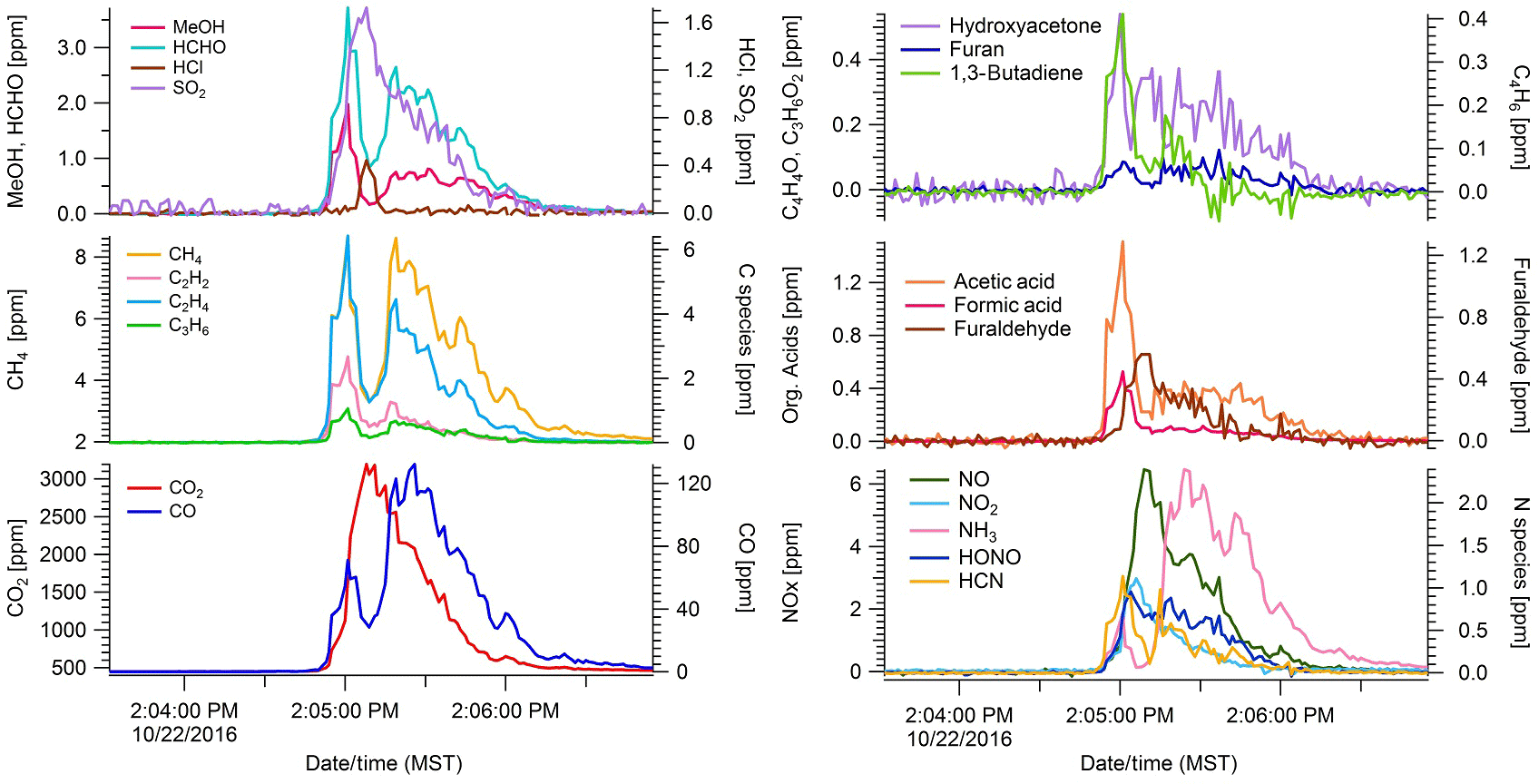
Figure 1Excess mixing ratios of 21 trace gases vs. time for a complete juniper canopy stack burn (no. 75) as measured using the OP-FTIR. CO2 denotes flaming; CO denotes smoldering. 1,3-Butadiene is shown as an example of lower signal-to-noise data but retained since there is no evidence of bias.
Mixing ratios were determined for carbon dioxide (CO2), carbon monoxide (CO), methane (CH4), acetylene (C2H2), ethylene (C2H4), propylene (C3H6), 1,3-butadiene (C4H6), formaldehyde (HCHO), formic acid (HCOOH), methanol (CH3OH), acetic acid (CH3COOH), glycolaldehyde (C2H4O2), furan (C4H4O), furaldehyde (C5H4O), phenol (C6H6O), hydroxyacetone (C3H6O2), water (H2O), nitric oxide (NO), nitrogen dioxide (NO2), nitrous acid (HONO), ammonia (NH3), hydrogen cyanide (HCN), hydrogen chloride (HCl), and sulfur dioxide (SO2). Mixing ratios were based on retrievals utilizing multicomponent fits to specific sections of mid-IR transmission spectra with a synthetic calibration nonlinear least-squares method (Griffith, 1996; Yokelson et al., 2007) applying both the HITRAN spectral database and reference spectra recorded at the Pacific Northwest National Laboratory (Rothman et al., 2009; Sharpe et al., 2004; Johnson et al., 2010, 2013). The above species were always or often enhanced in the smoke well above the real-time detection limits, but some species such as 1,3-butadiene, furaldehyde, phenol, and HCl were frequently not enhanced to more than 2–3 times the real-time detection limit and are not reported in those cases. The uncertainties in the individual mixing ratios varied by spectrum and molecule and were influenced by uncertainty in the reference spectra (1–5 %) or the real-time detection limit (0.5–20 ppb), whichever was larger. Typical stack concentrations ranged from hundreds of parts per billion to thousands of parts per million depending on the analyte (Fig. 1 and Stockwell et al., 2014).
2.3.2 Photoacoustic extinctiometers (PAX) at 870 and 401 nm
Particle absorption and scattering coefficients (Babs, Bscat Mm−1) were measured directly at 1 s time resolution using two PAXs (Droplet Measurement Technologies, Inc., Longmont, CO; Lewis et al., 2008), and SSA at 401 and 870 nm and the AAEs were derived using those measurements. A 1 L min−1 aerosol sample flow was drawn through each PAX using a downstream pump and split internally between a nephelometer and photoacoustic resonator for simultaneous measurement of light scattering and absorption. Scattering of the PAX laser was measured using a wide-angle reciprocal nephelometer that responds to all particle types regardless of chemical makeup, mixing state, or morphology. For absorption measurements, the laser beam was directed through the aerosol stream and modulated at a resonant frequency of the acoustic chamber. Absorbing particles transferred heat to the surrounding air, inducing pressure waves that were detected via a sensitive microphone. Advantages of the PAX include direct in situ measurements, a fast response time, continuous autonomous operation, and eliminating the need for filter collection and the uncertainties that come with filter artifacts (Subramanian et al., 2007).
We sampled stack burns through ∼ 2 m of 0.638 cm (o.d.) Cu tubing that ran from the stack to a splitter that connected the two instruments. From the splitter, each separate sample line encountered a scrubber to remove UV-absorbing gases such as NO2 (Purafil SP Media, minimum removal efficiency 99.5 %) and then a diffusion drier (silica gel 4–10 mesh) to remove water, with this order ensuring that both instruments were sampling at the same relative humidity (varying between 13 and 30 %). The scrubber and drier were refreshed before any signs of deterioration were observed (e.g., color change) and the diffusion-based designs should incur minimal particle losses, but losses were not explicitly measured. After the drier, each sample line featured a 1.0 µm size-cutoff cyclone and two acoustic notch filters that reduced noise. Both PAX instruments were calibrated before and after the experiment using the manufacturer-recommended scattering and absorption calibration procedures utilizing ammonium sulfate particles and a propane torch to generate pure scattering and strongly absorbing aerosols, respectively. The estimated uncertainty in PAX absorption and scattering measurements has been estimated as ∼ 4–11 % (Nakayama et al., 2015).
2.4 Emission ratios (ERs), emission factors (EFs), and modified combustion efficiency (MCE)
We convert the time series of mixing ratios for each analyte (Fig. 1) into a form that is broadly useful to others for implementation in local to global chemistry and climate models. For this, we produce emissions ratios (ERs) and EFs. The process starts by calculating excess mixing ratios (denoted ΔX for each species “X”) for all 23 gas-phase species measured using the OP-FTIR by subtracting the relatively small average background mixing ratio measured before each fire from all the mixing ratios observed during the burn. The molar ER for each species X relative to CO2 (ΔX∕ΔCO2) is the ratio between the sum of the ΔX over the entire fire relative to the sum of the ΔCO2 over the entire fire. A comparison of the sums is valid because the large entrainment flow ensures a constant total flow. Molar ERs to CO2 were calculated for all the species measured using the OP-FTIR for all 75 stack burns and the two most important room burns. For the other room burns, OP-FTIR data were generated only for CO2, CO, CH4, C2H4, C2H2, and H2O as losses in the room add uncertainty to the mixing ratios for many NMOGs, NH3, etc. The ERs to CO2 were then used to derive EFs calculated with the carbon mass balance (CMB) method, which assumes all of the burned carbon is volatilized and that all of the major carbon-containing species have been measured (Ward and Radke, 1993; Yokelson et al., 1996, 1999; Burling et al., 2010, Stockwell et al., 2014):
where FC is the measured carbon mass fraction of the fuel, MMx is the molar mass of species X, AMC is the atomic mass of carbon (12 g mol−1), NCj is the number of carbon atoms in each species j, and ΔCj or ΔX referenced to ΔCO2 are the source-average molar ERs for the respective species. The denominator of the last term in Eq. (1) estimates total carbon. Based on many BB combustion sources measured in the past, the species CO2, CO, and CH4 usually comprise 97–99 % of the total carbon emissions (Akagi et al., 2011; Stockwell et al., 2015). Our estimate of total carbon in this paper includes these three species and all the rest of the C-containing gases measured with the OP-FTIR as well as the C in the particles (i.e., BC and OC) based on the PAX data. Samples of each fuel component were analyzed for moisture content by weighing until dry and for C, H, N, S, and Cl by a commercial (ALS, Tucson) and an academic laboratory, whose results agreed well with each other on several overlapping fuel samples. The fire-average carbon mass fractions for mixed fuel beds were calculated from the average of the relevant fuel component analyses weighted by dry mass (Table S1). The usually small error in the CMB method caused by neglecting char formation (Bertschi et al., 2003) tends to be canceled by more complete combustion of the higher-C components (Santín et al., 2015) and both these effects are ignored here but will be explored in more detail in a companion study.
Two major combustion processes are often recognized for open burning of biomass: flaming and smoldering, where smoldering is an approximate term for all non-flaming processes (e.g., glowing and pyrolysis) as explored in more detail elsewhere (Yokelson et al., 1996; Koss et al., 2017). Combustion efficiency is the fraction of fuel carbon converted to carbon as CO2, which is maximized by flaming combustion, but the modified combustion efficiency (MCE) is also a useful approach for characterizing the relative amount of smoldering and flaming combustion by comparing the fuel carbon converted to CO2 versus CO2+ CO. Although the two processes often occur simultaneously throughout a fire, a high MCE (near 0.99) is an indication of nearly pure flaming, while a lower MCE (∼ 0.8) is an indication of nearly pure smoldering (Akagi et al., 2011) and an MCE of 0.9 would indicate roughly equal amounts of flaming and smoldering (i.e., a flaming ∕ smoldering ratio of ∼ 1):
In the PAX, the 870 nm laser is absorbed in situ by BC-containing particles only without filter or filter-loading effects that can be difficult to correct. We directly measured aerosol absorption (Babs, Mm−1) and used the literature-recommended mass absorption coefficient (MAC) (4.74 ± 0.63 m2 g−1 at 870 nm) to calculate the BC concentration (µg m−3) (Bond and Bergstrom, 2006), but the BC mass can be adjusted using different MAC values if supported by future work. Because the PAXs also measured light scattering, scattering and absorption values can be combined to directly calculate the SSA (the ratio of scattering to total extinction). SSA is a useful input for climate models, where an SSA closer to 1 indicates a more “cooling” highly scattering aerosol:
To a good approximation, sp2-hybridized carbon (including BC) absorbs light proportional to frequency (Bond and Bergstrom, 2006). Thus, the Babs contribution from BC at 401 nm can be calculated from 2.17 times Babs at 870 nm, and any additional Babs at 401 nm can be assigned to BrC subject to limitations due to “lensing” by coatings discussed elsewhere (Pokhrel et al., 2016, 2017; Lack and Langridge, 2013; Lack and Cappa, 2010). Pokhrel et al. (2017) found that coatings typically accounted for much less than 30 % of absorption in room burn smoke 1–2 h old and coatings are likely much less important in 5 s old stack burn smoke (Akagi et al., 2012). Coating effects are very difficult to deconvolve from BrC effects even with additional instruments that were not available during the stack burns (Pokhrel et al., 2017). This adds some uncertainty to the BrC attribution (±25 %) but not to the absorption measurements themselves. Absorption by the BrC component of OA means that an approximate mass of OA can be calculated using an OA MAC of 0.98 m2 g−1 (Lack and Langridge, 2013), but the MAC for OA is variable because BrC chemistry and BrC ∕ OA vary and the OA MAC is also highly dependent on the BC ∕ OA ratio as described elsewhere (Saleh et al., 2014). We use the qualitative OA to calculate a small term in our CMB method that helps account for unmeasured C species (assuming OA ∕ OC of 1.6), but we do not report OA or OC in the tables as quantitative species. Critically though, we do report the OA absorption due mainly to BrC at 401 nm, a poorly characterized term that needs to be improved in climate models to better estimate the radiative forcing of BB aerosol (Feng et al., 2013). The mass ratio of BC to the CO2 measured using the FTIR was multiplied by the EFs for CO2 to determine mass EFs for BC (g kg−1). The EFs for absorption and scattering optical cross sections at 870 and 401 nm (EFabs, EFscat) were calculated from the measured ratios of Babs and Bscat to CO2 and reported in units of square meters per kilogram of dry fuel burned. EFabs or EFscat are more precisely the optical cross-section (m2) due to the particles produced when a kilogram of fuel is burned if the emissions are mixed into a cubic meter of air. These EFs enable direct calculation of the absorption or scattering coefficient (m−1) by multiplication with a specified ratio of fuel burned to a volume of air (kg m−3) (Bond et al., 1999; Moosmüller et al., 2005). We also report the estimated portion of Babs at 401 nm due to BrC. Finally, the AAE (401 and 870 nm) can be calculated from the 401 and 870 nm data, where the AAE of pure BC is close to 1 and larger values are indicative of smoke absorption more dominated by BrC emissions:
The AAE is useful as an indicator of BrC ∕ BC, but in addition, the full aerosol absorption spectrum is often approximated with a power-law function (absorption = C × λ−AAE) and thus the AAE determined with any wavelength pair can be used to approximately calculate the shape of absorption across the UV–VIS range (Reid et al., 2005).
Table 1Average emission factors (g kg−1) of common western US ecosystems measured in the lab.
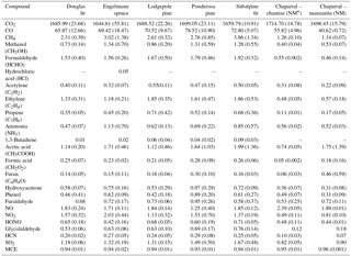
Values in brackets are (1σ) standard deviation. * “NM” indicates the relatively unpolluted North Mountain sample collection site.
3.1 Overview of wildfire trace gas emissions
We sampled a total of 75 stack burns and 32 room burns at the FSL combustion facility during October and November 2016. Figure 1 shows temporal profiles for the excess mixing ratios of 21 gas-phase compounds (not including water) measured with the OP-FTIR for a complete juniper canopy fire (fire 75). Immediately after ignition, the fire is characterized by a large increase in CO2, corresponding to flaming, followed by a slower increase in CO from smoldering combustion. As is common to most fires, there is no clear distinction between flaming and smoldering but rather an evolving mix of the two processes. Fire-integrated ERs to CO2 and EFs were determined for all 75 stack fires based on the whole fire. For room burns, we calculated EF based on integrating the ΔX only up to the point at which emissions were well mixed to capture the whole fire but also minimize the effect of wall losses and infiltration (see Fig. 3 in Stockwell et al., 2014). The fire-integrated EFs for some of the most common western US ecosystem fuel complexes sampled in this study are summarized in Table 1. These are averages of the replicate fires (three to four replicate measurements for each fuel type). Table 1 does not reveal a strong ecosystem dependence across the coniferous ecosystems but does indicate lower EFs for many pollutants emitted by the chaparral fires. However, large wildfires often burn in multiple fuel types simultaneously. For instance, the Rim Fire burned in pine, pine–oak, and chaparral fuels simultaneously (Liu et al., 2017). These factors justify using a single set of EFs for all wildfires, unless detailed fuel data are available that warrant more precise EF estimates. The derivation of the best wildfire EFs is explored in more detail in the next section. A summary of all the EFs we measured with OP-FTIR and PAX can be found in Table S2, with the averages of specific fuel components and complexes found in Table S3. Numerous additional NMOGs that were measured using other instruments (e.g., H3O+ chemical ionization mass spectrometer (CIMS) and I− CIMS) will be presented elsewhere (Koss et al., 2017). These additional species are often reactive and very important in plume chemistry even though they have only a small effect on the carbon mass balance. A few species were measured with both OP-FTIR and MS and the preferred values depend on several issues such as S ∕ N (often better on MS), interference (often worse on MS), “stickiness”, fragmentation, and proton affinity that are discussed in more detail elsewhere (Koss et al., 2017).
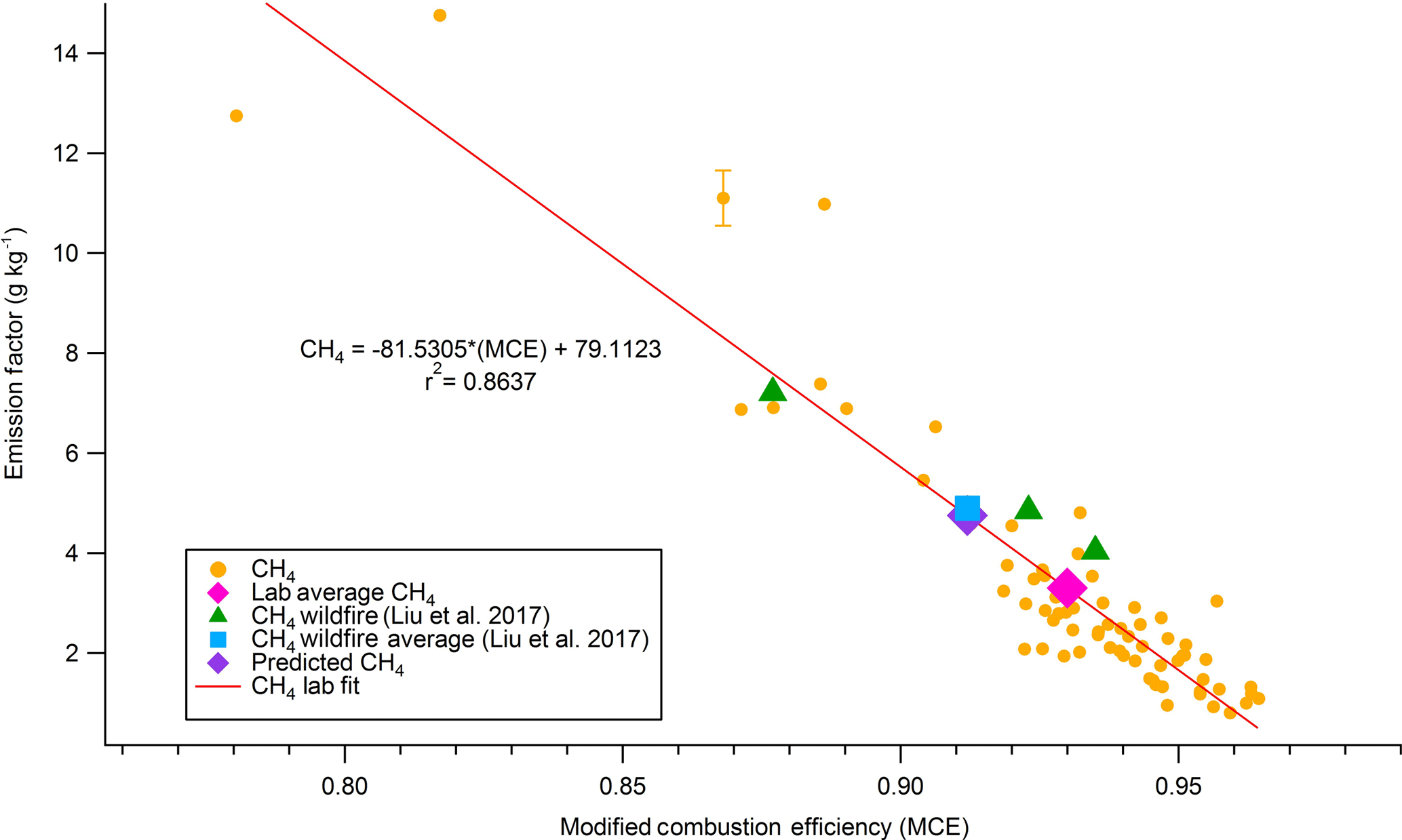
Figure 2Methane emissions from 75 stack fires plotted against corresponding MCE and wildfire field methane emissions plotted against corresponding wildfire field MCE. Also included are the field-average methane emissions (blue) and the predicted methane emissions (purple) using the linear regression shown and a field-average MCE of 0.912.
3.2 Comparison of laboratory EF to wildfire EF
It is important to compare our FIREX laboratory fire emissions data to field measurements of real wildfires to assess how representative and useful the lab-based data are, especially for the many species measured in the laboratory but not the field. We assess representativeness by comparing the EF results for species measured in both the field and our laboratory fires. EF measurements on real wildfires are rare, but Liu et al. (2017) report recent EFs for three wildfires sampled during the 2013 Studies of Emissions and Atmospheric Composition, Clouds, and Climate Coupling by Regional Surveys (SEAC4RS, https://espo.nasa.gov/missions/seac4rs) (Toon et al., 2016) campaign, and the Biomass Burning Observation Project (BBOP, https://www.arm.gov/research/campaigns/aaf2013bbop) campaign.
Table 2Summary of the comparison of emission factors (g kg−1) measured in the lab and field.
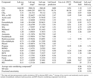
a The slope and intercept parameters enable calculation of EF at alternate MCE values. b Average of less reactive and moderately reactive species: includes formaldehyde, methanol, hydroxyacetone, and HCN. Reactive smoldering compounds were left out.
We compare our results from the FSL combustion studies to those reported by Liu et al. in two ways. In method 1, we plot the lab-measured EFs against their corresponding MCEs for all the fires and we fit the data with a linear regression relationship for each compound. Using the slope and y intercept of the linear regression, and the field-average MCE from Liu et al. of 0.912, we calculate a lab-based prediction of EF at the field-average MCE for each compound measured with the OP-FTIR. Figure 2 shows an example of the procedure for CH4, comparing the lab-predicted EF at the field-average MCE (4.76 g kg−1) to the average field-measured wildfire EF (4.90 g kg−1). In method 2, we compared the simple lab-average EF to the average field-measured wildfire EF. The results of these two methods are shown in Table 2 and Fig. 2. Method 1 is generally preferred because the laboratory fires had a higher average MCE (i.e., a higher fire-integrated flaming ∕ smoldering ratio) than the real wildfires sampled to date, most likely due to some unavoidable drying of the fuels during storage and some underrepresentation of the largest diameter fuels (Table S1). The differences between the laboratory prediction at the field-average MCE and the field-average emissions are probably mostly due to the relative age of the smoke and the reactivity of compounds. The field study included smoke samples up to 2 h old and elevated OH, HO2, H2O2, O3, etc. have been observed in fresh smoke plumes (Hobbs et al., 2003; Yokelson et al., 2009). Thus the more reactive species (e.g., SO2, HCl, NOx, and some NMOGs) have lower EFs in the field data. For example, the lab ∕ field ratio increases going from ethylene to propene to 1,3-butadiene in accordance with, though not directly proportional to, their increasing OH rate constants, and other chemistry, instrumental, and sampling challenges are relevant for some species (e.g., Finlayson-Pitts and Pitts, 2000; Apel et al., 2003; Fig. 7 in Hornbrook et al., 2011; Burkholder et al., 2015). A few reactive species were measured in two older airborne studies of fresh western US wildfire smoke and they agree significantly better with our lab-based predictions (Radke et al., 1991; Hobbs et al., 1996). For instance, Radke et al. (1991) report EFs for NOx as NO (2.0 g kg−1), NH3 (2.0 g kg−1), and C3H6 (0.70 g kg−1) for the Myrtle–Fall Creek wildfire that are all within 20 % of our lab-predicted EFs. Hobbs et al. (1996) report an EF for SO2 (0.79 g kg−1) that is closer to our value than the Liu et al. value is despite the much lower MCE (0.81).

Figure 3Comparison of the lab-predicted EFs at the field-average MCE to average field-measured EFs reported by Liu et al. (2017).
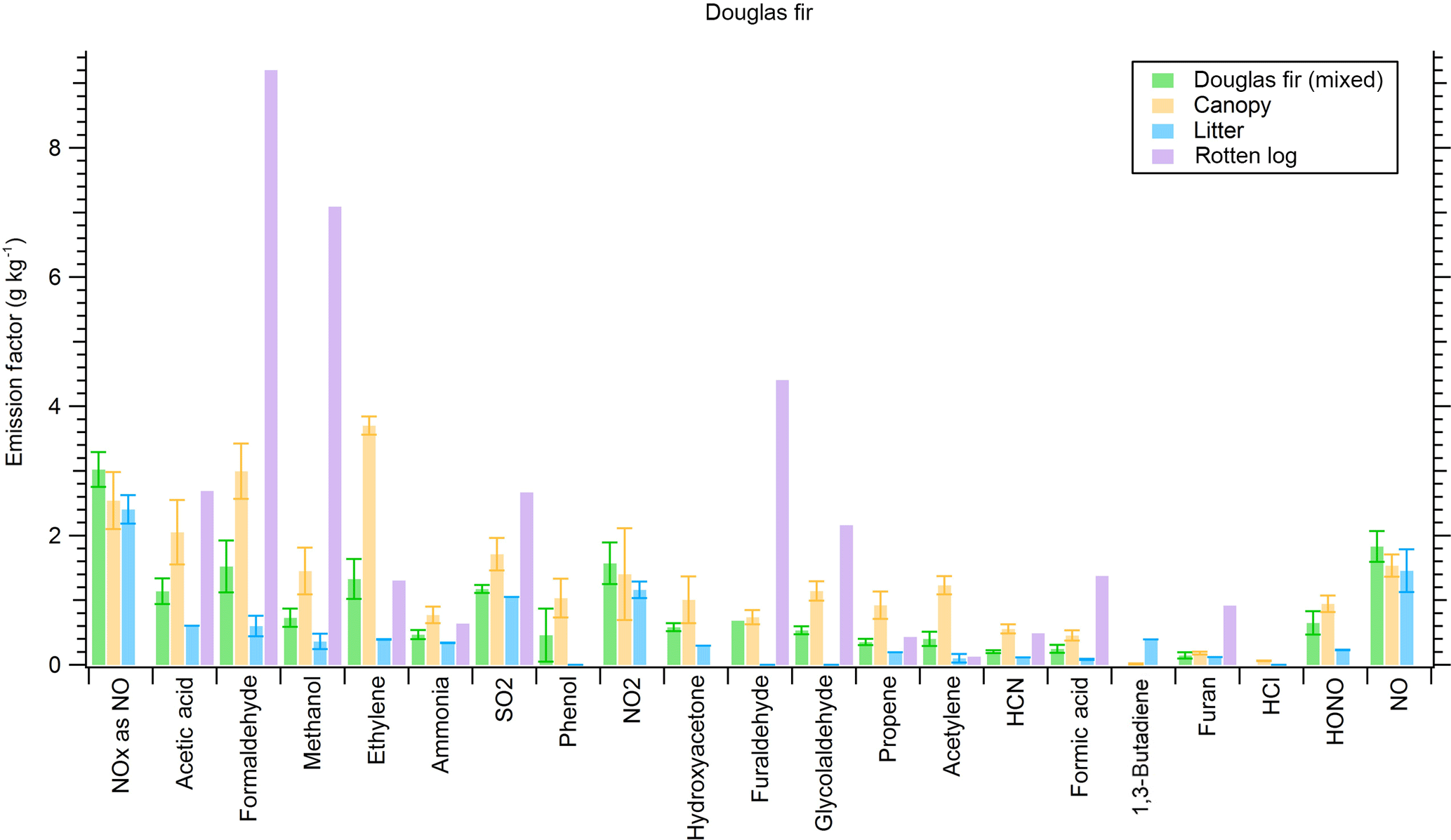
Figure 4Trace gas emissions from a mixed Douglas fir ecosystem (including sound and dead wood, but rotten log not included) and pure components. Sound dead wood was not burned separately except as untreated lumber.
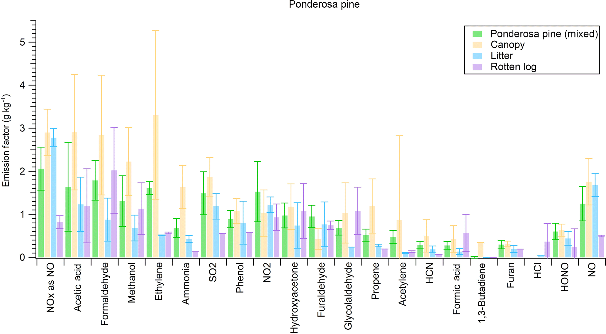
Figure 5Trace gas emissions from a mixed ponderosa pine ecosystem (including sound dead wood; rotten log not included) and pure components.
Figure 3 shows the comparison for method 1 from Table 2 graphically. From Fig. 3 it is clear that for the main relatively stable compounds, including formaldehyde, methanol, and hydroxyacetone, the lab-predicted EF falls within 21 % of the measured wildfire EF and all the emissions except NOx and SO2 overlap within the observed variability. Also highlighted in Fig. 3, many compounds such as HONO, acetic acid, ammonia, phenol, glycolaldehyde, formic acid, etc. were measured only for our laboratory fires. The lab-measured EFs for these OP-FTIR species and the data for many NMOG species measured by MS and FIREX data in general can thus be used to generate representative EFs or other data for real wildfires. Many of these EFs are critically important to represent wildfire emissions well: e.g., NH3 (Benedict et al., 2017) and secondary organic aerosol or peroxyacetyl nitrate precursors (Alvarado et al., 2015; Müller et al., 2016). Other approaches to generate representative data that are not explored in detail here but should work well include reporting the average for the laboratory fires clustered around the field-average MCE (fires 8, 39, 45, 51, 59, and 66) or reporting ER to CO (e.g., Koss et al., 2017), where the latter can also be converted to EF by coupling with the field-average EF of CO. For example, if we take the average of six fires clustered around the field-average MCE in the new CH4 plot shown in Fig. 2, we get an average EF for CH4 of 4.67, which is close to the value of 4.90 reported by Liu et al. Alternatively, we can calculate a molar ER for CH4 to CO for all the laboratory fires (0.108), then utilize the wildfire-average EF of CO reported by Liu et al. (89.3 g kg−1) to calculate a new EF. Using this method, we get an EF for CH4 of 5.5, which is within 11 % of the field-average value. Either of these methods should help reflect the field-average flaming ∕ smoldering ratio. In addition, positive matrix factorization was found to be useful to model field and laboratory EFs for NMOGs as discussed elsewhere (Sekimoto et al., 2018). Finally, given the small amount of field sampling, more field work is clearly needed.
3.3 EF dependence on fuel
We burned individual fuel components (duff, litter, canopy, etc.) in addition to mixtures of major components found in widespread western US coniferous ecosystems for insights into fuel effects on emissions and to what degree specific emissions were enhanced by a certain component. For example, Fig. 4 shows the EFs of 21 trace gases from the Douglas fir ecosystem fuel mixture burns side by side with the EFs from burning pure Douglas fir components in separate fires. Emissions of furaldehyde, formaldehyde, and methanol were enhanced when burning a pure rotten log component, while acetylene, ethylene, and propene, as well as other non-methane hydrocarbons (NMHCs), were more prevalent in emissions from Douglas fir canopy. We did the same analysis for a ponderosa pine ecosystem (Fig. 5). While the canopy component in ponderosa pine produced enhanced emissions of NMHCs, the rotten log did not contribute to the same level of enhancement in furaldehyde, formaldehyde, and methanol because of a transition to flaming combustion during the second half of the fire. Additionally, we observed an enhancement in NOx emissions from the litter and canopy components in ponderosa pine. Coniferous ecosystem values are fairly similar for both fuels and agree within 30 % for the majority of compounds, excluding methanol, furan, and NOx. We also note that while the mixed Douglas fir and ponderosa pine ecosystem fuel mixtures that we burned contained canopy, litter, and woody components in varying diameter classes, they did not contain a rotten log since the latter component is not included in FOFEM. We further investigate fuel variability by taking pure components from several ecosystems and comparing them to one another. Figure 6 shows species emitted by duff from three different coniferous ecosystems. Acetic acid and methanol are strongly emitted by all three duff fuels, but ammonia enhancement occurs in only Engelmann spruce and subalpine fir fuels. Jeffrey pine duff had a lower EF for NH3 despite similar fuel N. This could possibly be due to the age of the fuel as it was contained in storage longer than other fuels and not fresh. Additional results for other fuel components (rotten log, canopy, litter) are in Figs. S1, S2, and S3, respectively.
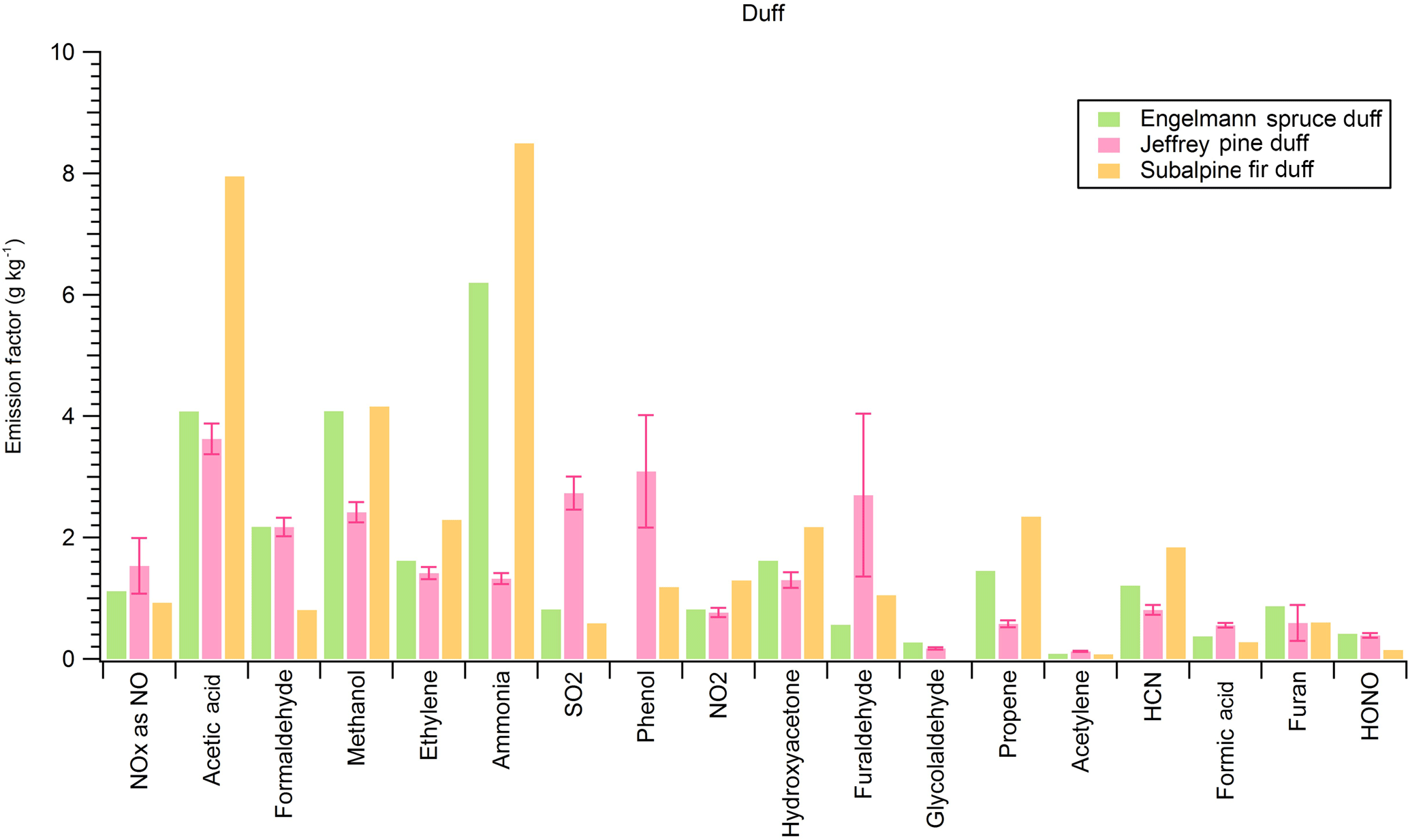
Table 3Lab-average emission factors (m2 kg−1) and fire-integrated optical properties for common western US ecosystems.
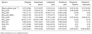
Values in brackets are (1σ) standard deviation.
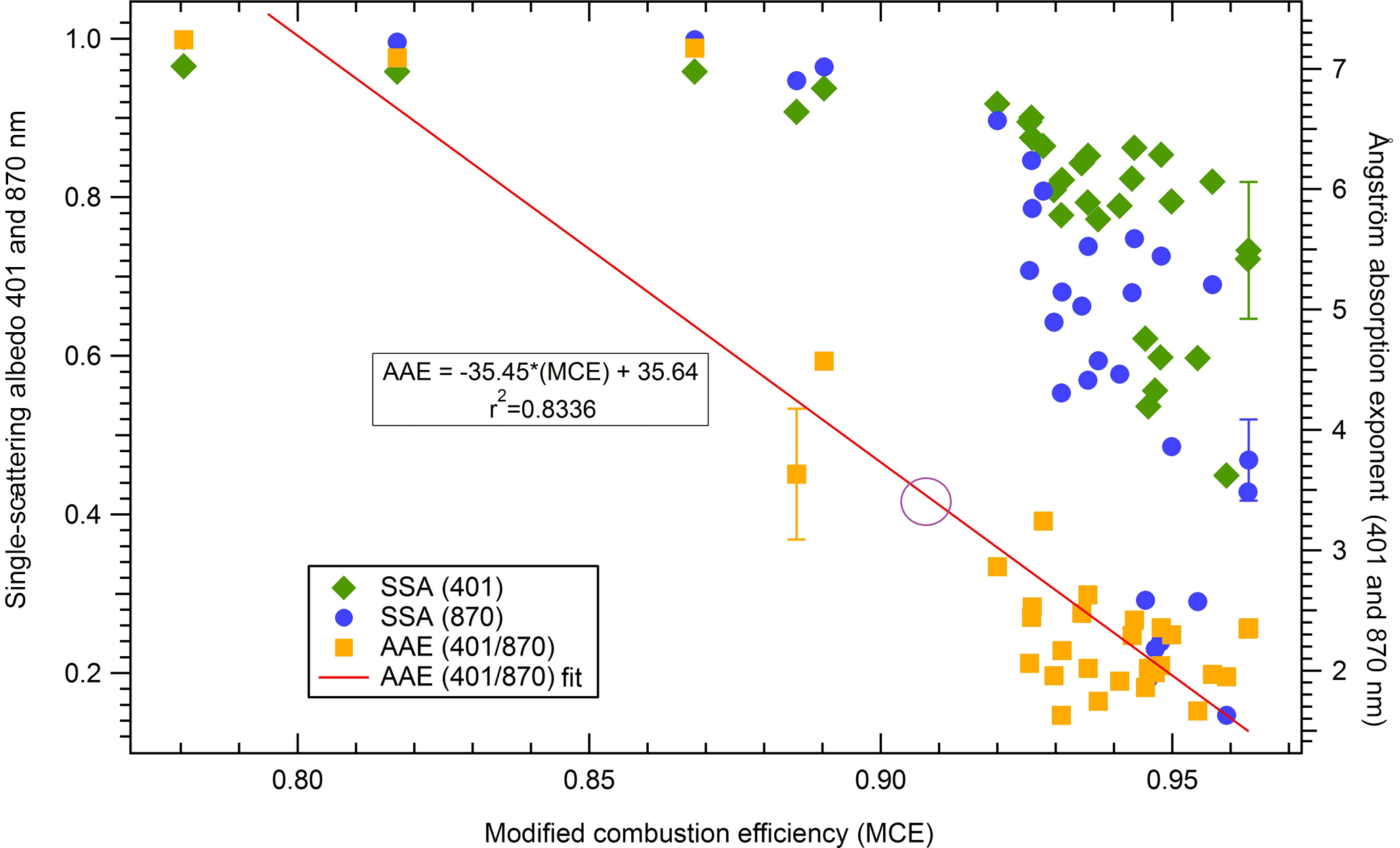
Figure 7SSA at both wavelengths (401 and 870 nm) and AAE (401 and 870 nm) against MCE for 31 stack fires for which both 401 and 870 nm data were available. The circle on the fit line represents the lab-predicted AAE using the wildfire field-average MCE of 0.912. SSA is difficult to fit to MCE and fits better to EC and OC data, which were not available (Liu et al., 2014; Pokhrel et al., 2016).
3.4 Overview of optical properties
As mentioned previously, we measured absorption and scattering coefficients directly at 401 and 870 nm. For the first 31 stack fires, which included most of the studied fuel types, we have both 401 and 870 nm data. For the remaining 44 stack fires, we only report data at 870 nm as we used our 401 nm PAX for intercomparison studies that will be reported elsewhere. Figure 7 plots the AAE and SSA at both wavelengths of 31 stack fires as a function of MCE. High AAE is an indicator of BrC and relates to smoldering, which is denoted by low MCE and high SSA values. Smoldering is also associated with higher EFs for OA, most NMOGs, and other gases such as NH3. Low AAE, along with low SSA and high MCE values, indicates more flaming combustion, which is also generally associated with higher EF for BC and “flaming compounds” such as CO2, NOx, and SO2. The lab-based average fire-integrated optical properties for some of the most common western US ecosystems are listed in Table 3. Table 3 does not reveal a strong ecosystem dependence among coniferous ecosystems tested for optical properties but does indicate that chaparral fire aerosol has consistently lower SSA than coniferous fire aerosol and that there are significant contributions of absorption by BrC at 401 nm among all ecosystems. The absorption by BrC is responsible for at least half and up to two-thirds of the absorption at 401 nm even at higher MCE. The laboratory-average AAE of 2.80 ± 1.57 across all 31 fires confirms a role for BrC, while the lab-average SSA at both wavelengths indicates the fresh lab-fire aerosol would have a net warming influence in the atmosphere (SSA < 0.9; Praveen et al., 2012), although SSA can increase with smoke age (Yokelson et al., 2009). The absorption of BrC at 401 nm has several implications in atmospheric chemistry, including impacts on UV-driven photochemical reactions producing ozone, and the lifetime of NOx and HONO. Furthermore, because of its absorbing nature, factoring in the BrC could mean the net radiative forcing of BB is not cooling or neutral as often assumed, but warming if the BrC is sufficiently long-lived as probed in other FIREX studies and previous papers (e.g., Feng et al., 2013; Forrister et al., 2015).
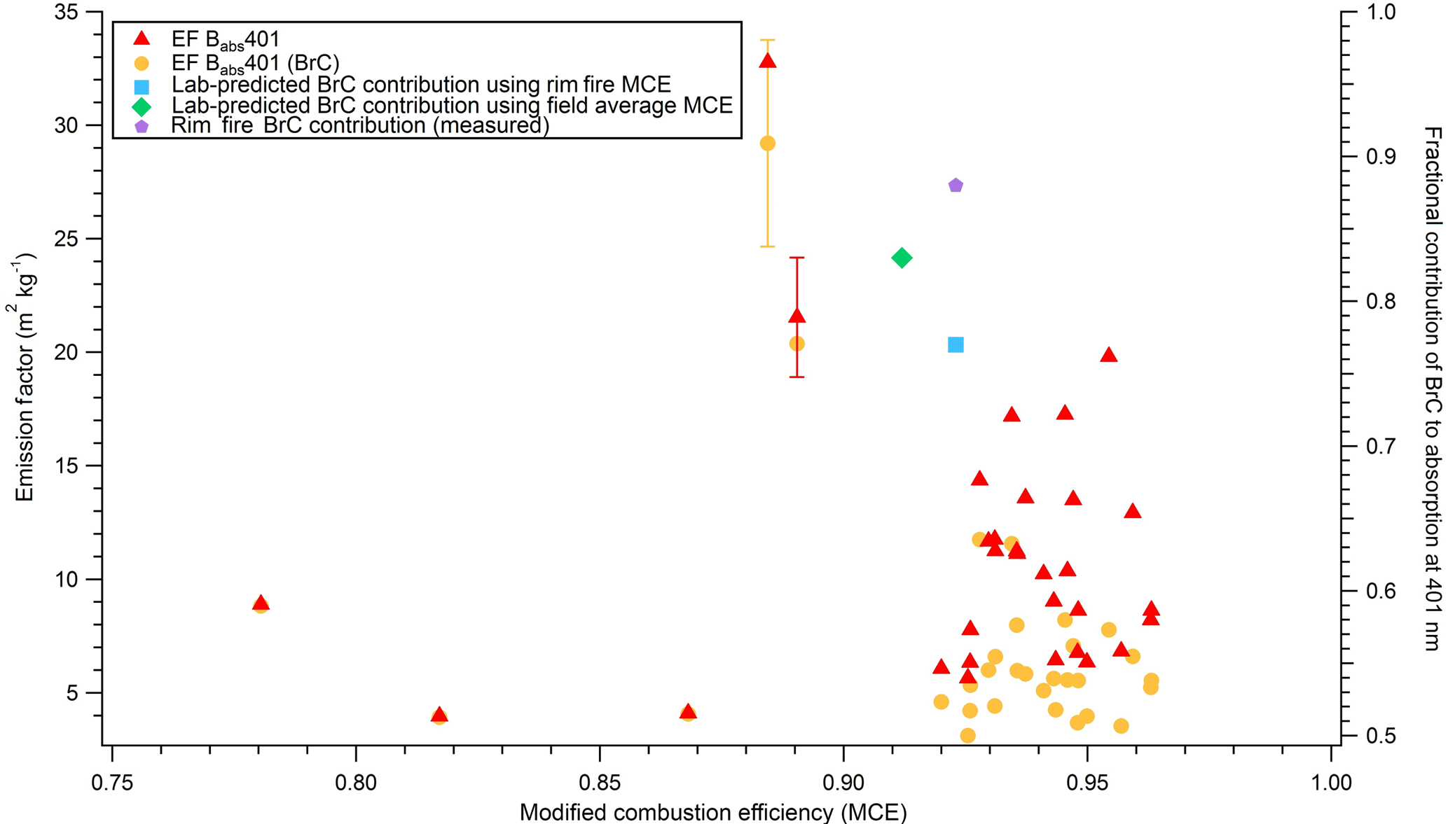
Figure 8Absorption emission factors measured at 401 nm for “BC plus BrC” and for “BrC only” for 31 lab fires, Also shown are the fractional contributions of BrC to total absorption at 401 nm predicted from the lab AAE data at the field-average MCE (green), the Rim Fire MCE (blue), and the field-measured AAE (purple) (Forrister et al., 2015; Liu et al., 2017).
3.5 Comparison of laboratory optical properties to field optical properties
There are very few field measurements of the optical properties of smoke from US wildfires, but we can compare our results from the laboratory studies to the initial aerosol optical properties for one wildfire (the Rim Fire) reported by Liu et al. (2017) and Forrister et al. (2015). An AAE of 3.75 at an MCE of 0.923 for the Rim Fire is reported between these two studies. With the linear regression of the laboratory data shown in Fig. 7, we can predict an AAE of 3.31 at the wildfire field-average MCE (0.912) and an AAE of 2.91 at the Rim Fire MCE (0.923) using prediction method 1 described in Sect. 3.2. At the wildfire field-average MCE, our calculated AAE represents 88 % of the reported Rim Fire AAE, while at the Rim Fire MCE, our calculated AAE represents 78 % of the reported Rim Fire AAE. Although our calculated values are relatively close to the reported value, a small change in AAE implies a big change in the BrC ∕ BC absorption ratio, but only a small change in the percentage of absorption by BrC. Our AAE values imply that BrC accounts for 77 to 82 % of the absorption at 401 nm. The average of the AAE from the single Rim Fire measurement (3.75) and the AAE predicted from the more extensive laboratory fires (3.31) is ∼ 3.5, which may be a reasonable best guess at the AAE of fresh US wildfire smoke and implies that ∼ 86 % of absorption at 401 nm is due to BrC.
Table 4Summary of the comparison of optical properties and emission factors (m2 kg−1) measured in lab to the Rim Fire.
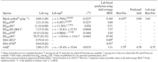
a Values in brackets are (1σ) standard deviation. b Average for all 75 stack fires for which 870 nm data are available. c Average for 31 fires for which both 401 and 870 nm are available. d SSA values calculated from Babs and Bscat EF. e Value not published (X. Liu, personal communication, 2017; https://www.nasa.gov/mission_pages/seac4rs/index.html). f From Forrister et al. (2015). g The low r2 equations return reasonable values at the field-average MCE. h In the equations below, “y” is the quantity in column 1 and “x” is MCE.
In Fig. 8, we plot the initial percentage of absorption by BrC at 401 nm for the Rim Fire measured AAE and for our lab-estimated AAE at the field-average MCE. Figure 8 also shows the lab-measured total EFabs401 and the BrC contribution to EFabs401 for 31 laboratory fires. BrC dominates absorption at 401 nm at low MCE values, and as MCE increases, BrC absorption remains a significant but variable component of overall absorption. The variability is likely due to realistic “natural” fire-to-fire variability in fuels, moisture content, etc.
In Table 4 we report the study averages for BC mass EF, absorption and scattering EFs, SSA, and AAE. The quantities that require 401 nm data are averages for the 31 stack fires for which 401 and 870 nm data were obtained, while the quantities that need just 870 nm data are averages for all 75 stack fires. We also show the comparison of our lab-average and lab-predicted AAEs to the AAE in Forrister et al. (2015) and our lab-average and lab-predicted BC EF to the unpublished BC EF calculated as part of Liu et al. (2017). Table 4 also presents a set of equations that can be used to fit lab-measured optical properties and make predictions at any MCE. However, more measurements of wildfires in the field and the laboratory (including aging) are needed to asses wildfire aerosol optical properties.
Table 5Optical properties and emission factors (m2 kg−1) for mixed coniferous ecosystems and ecosystem components.
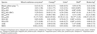
a Douglas fir, Engelmann spruce, lodgepole pine, ponderosa pine, subalpine fir. b Douglas fir, Engelmann spruce, lodgepole pine, ponderosa pine, juniper, subalpine fir. c Douglas fir, loblolly pine, lodgepole pine, ponderosa pine, subalpine fir. d Engelmann spruce, Jeffrey pine, ponderosa pine, subalpine fir. e Engelmann spruce. f Douglas fir, ponderosa pine.
3.6 Fuel dependence of aerosol optical properties
Burning individual fuel components in addition to mixtures found in typical, widespread western US ecosystems allows us to investigate the extent to which optical properties are either enhanced or diminished by certain components. Table 5 lists the study-average BC EF and optical properties for all the coniferous ecosystems shown in Table 3 and the study-average BC EF and optical properties for the individual fuel components averaged across all the coniferous ecosystems. The averages and standard deviations for each reported quantity indicate that there is large variation among specific components and a large coefficient of variation for the coniferous ecosystem average. The variability could potentially depend on ecosystem type, fuel components, fuel moisture, or other things as discussed for trace gases in section 3.3. While there is considerable variation within each ecosystem type, the individual ecosystem averages in Table 3 all agree within 38 % of the study average for all the coniferous ecosystems shown in Table 5 and the AAEs are all within 20 %. However, Table 5 also shows that the average AAE for some ecosystem components is very different from the average AAE for all the coniferous ecosystems (2.26). For instance, the largest contribution to a high AAE per fuel component consumed comes from duff, where BrC accounts for almost all of the absorption at 401 nm (AAE 7.13). The rotten log component also contributes an anomalously high average AAE of 4.60. Thus, these components contribute more BrC relative to BC in proportion to their fuel consumption to the mixed ecosystem results, where AAE is 2.26 and BrC accounts for just over half of the absorption at 401 nm. Conversely, litter consumption would tend to lower a fuel mixture's AAE. However, AAE is a measure of the shape of the aerosol absorption cross section and the absorption EFs are a measure of total emissions of absorbing material. In this respect, litter produces more BC absorption and more BrC absorption per unit mass than duff though at a lower BrC ∕ BC ratio than duff. This is consistent with the lower SSA for litter. We conclude that the variability in mixed ecosystem optical properties was likely due to variable consumption of pure components, with a weaker dependence on the dominant tree species. For example, much of the variability in ecosystem-average AAEs and the study-average AAE is linked to the varying amount of duff consumed in the mixed fuel beds (Table S1). (The variability in actual duff consumption is likely larger than the variability in duff loading shown as the amount of residual material also varied.) Duff consumption in the field is increased by drought conditions, which would contribute to variability in real fires (Davies et al., 2013).
We can compare our duff results to previous measurements of optical properties of duff-fire aerosol by Chakrabarty et al. (2010). These authors identified tar balls as a major BrC species produced by duff combustion and they measured an AAE of 4.2 (405 and 532 nm wavelength pair) for a ponderosa pine duff sample from MT. Including their other duff sample (Alaskan feather moss duff), they obtained a study-average duff-combustion AAE of 5.3. We measured AAE on two much larger burns (∼ 4 times more fuel mass, fire nos. 12 and 26) in Engelmann spruce duff, with different wavelengths, and at much lower MCE (0.843 ± 0.036 versus ∼ 0.91). We obtained a study-average duff combustion AAE of 7.13 (0.057). Both studies observed a high AAE for duff combustion. Their lower AAE values could be related to different wavelengths used, the possibility of some BrC absorption at 532 nm (Bluvshtein et al., 2017), the different duff type, and/or their higher MCE, which they attributed to sampling some flaming combustion during the ignition process. The AAE calculated from our AAE versus MCE fit (for all fuels) at their MCE of 0.91 is relatively closer to their value.
In summary, the results presented indicate that, in all cases, burning a typical ecosystem mixture of components produces a significant amount of BrC. As mentioned previously, this has several implications in regional atmospheric chemistry and radiative forcing. Additional instruments were deployed on room burn experiments, in which the fuels were also purposely changed to investigate the effect on optical properties and the results will be reported elsewhere (e.g., Manfred et al., 2018).
3.7 Trace gas and BC emissions of peat, dung, and rice straw combustion
We also measured emissions from several fires of peat, rice straw, and dung due to their widespread burning in Asia and their value as extreme examples of fuel impacts (e.g., high smoldering-to-flaming ratio or high N or Cl content). Peat, which is especially important in Southeast Asia (Stockwell et al., 2016a) is similar to duff found in the western US in that it is often consumed by pure smoldering combustion and produces high AAE (Pokhrel et al., 2016), high HCN emissions, and low BC emissions. Although we did not measure the AAE for our peat fire aerosol, we do report an MCE of 0.83, where a low MCE likely indicates a high AAE. We also report EFs for CH4 (10.39 g kg−1), HCN (3.97 g kg−1), acetic acid (4.44 g kg−1), and BC (0.003 g kg−1). We compare these values to the field measurements reported in Stockwell et al. (2016a): CH4 (9.51 ± 4.74 g kg−1), HCN (5.75 ± 1.60 g kg−1), acetic acid (3.89 ± 1.65 g kg−1), and BC (0.006 ±0.002 g kg−1) and find that our values agree well (EF of BC extremely small compared to most BB (Akagi et al., 2011) and gases within 31 %) between peat fire measurements in the laboratory and the field. (A more detailed comparison will follow planned field measurements.)
Additionally, we compare our dung MCE (0.90), CH4 (6.63 g kg−1), HCN (1.96 g kg−1), acetic acid (6.36 g kg−1), and BC (0.01 g kg−1) values to those based on field work in Nepal reported in Stockwell et al. (2016b): MCE (0.90), CH4 (6.65 ± 0.46 g kg−1), HCN (2.01 ± 1.25 g kg−1), acetic acid (7.32 ± 6.59 g kg−1), and BC (0.004 ± 0.003 g kg−1). We find excellent agreement between our values (15 % for trace gases and a very small EF of BC) and those reported from field measurements in Nepal.
Rice straw was burned because of its global importance in agricultural waste burning and to probe the extremes of fuel chemistry (Akagi et al., 2011). Grasses are usually very high in chlorine content (0.61 %, Table S1; Lobert et al., 1999) and our EF for HCl of 0.65 g kg−1 for rice straw was the highest of any fuel measured during the FIREX campaign. Furthermore, our rice straw EF for HCl is comparable to Stockwell et al. 2015 (0.43 ± 0.29). The findings briefly summarized in this section further suggest and reinforce the idea that simulated laboratory fires can probe fuel effects and provide an accurate representation of measurements in the field, even outside the scope of western US wildfires. More comprehensive, recent discussions of these fuels can be found elsewhere (Stockwell et al., 2016a, b; Jayarathne et al., 2018a, b).
We measured trace gas and aerosol emissions from 107 simulated western wildfires during the FIREX campaign in the fall of 2016 using OP-FTIR and PAX. For 31 stack fires, we report aerosol measurements based on both 401 and 870 nm, and for the remaining 44 stack fires we report aerosol characteristics based on only 870 nm data. We provide the MCE and the mass EF (g kg−1) for 23 different trace gases (not including water) and BC. We also provide the scattering and absorption EF (m2 kg−1) at 870 and 401 nm along with the EFabs401 due to BrC only, SSA, and AAE. We burned canopy, litter, duff, dead wood, and other fuels in combinations using FOFEM to represent relevant ecosystems and as pure components to investigate the effects of individual fuels. Full trace gas data are reported for all 75 stack burns and two room burns, and CO2, CO, CH4, C2H4, C2H2, and MCE were archived for the remaining room burns. We found little variability in average trace gas EFs across coniferous ecosystems, but the average EFs for two chaparral plant species were similar to each other and lower than in coniferous ecosystems for most pollutants, including CH4 (1.20 ± 0.09 g kg−1), formaldehyde (0.50 ± 0.06 g kg−1), glycolaldehyde (0.15 g kg−1), and HCN (0.09 g kg−1) to name a few. Additionally, there was considerable variability in the average trace gas EF for certain fuel components. For instance, emissions of some NMOGs were enhanced from a Douglas fir rotten log and emissions of NOx were enhanced from ponderosa pine litter and canopy components.
In a similar fashion, there was little variation in the average optical properties for the different mixed coniferous ecosystems, but individual fuel components like duff and rotten logs contributed significantly on a per mass basis to the relative importance of BrC and BC, with BrC accounting for nearly 100 and 94 % of the absorption at 401 nm for these fuel components (using data only from fires with measurements at two wavelengths).The lab-average AAE for all 31 fires, including those burning components like chaparral and coniferous canopy, which tend to burn more by flaming, was 2.8 (Table 4), indicating that BrC absorption contributed to over half (64 %) of the absorption at 401 nm for the laboratory fires on average.
We compared the trace gas and aerosol emissions from the fires in our laboratory-simulated western US ecosystems to those from real western US wildfires measured in slightly aged smoke in the field as reported by Liu et al. (2017) and Forrister et al. (2015). Despite some underrepresentation of the largest diameter fuel class we were able to use a simple procedure to account for the flaming-to-smoldering ratio and generate EF values from the laboratory data that were in agreement with the field data for most “stable” trace gases, including CH4 (within 3 %), formaldehyde (within 5 %), methanol (within 21 %), and hydroxyacetone (within 2 %). Most of the EF discrepancies were due to the field smoke being more aged. The excellent agreement suggests that FIREX data can be confidently used in general to represent real fires, especially for species not measured yet in the field. For instance, important compounds rarely or not previously measured in the field for western wildfires but measured in this study include ammonia (1.62 g kg−1), acetic acid (2.41 g kg−1), HONO, and others (Fig. 3). Optical properties were not compared as extensively because limited field data are available, which highlights the need for more field measurements on true wildfires. However, a preliminary best guess for a fresh wildfire smoke AAE of ∼ 3.5 is supported by averaging the lab-based predictions and the more limited field data. Impacts on photochemical reactions producing ozone and the lifetime of NOx and HONO are likely as a result of the strong abundance of BrC. In addition, recognizing the presence of absorbing BrC in BB plumes could alter the modeled contribution of BB to net radiative forcing in a more positive direction. Finally, to investigate fuel chemistry impacts and due to their widespread global importance, we also measured EFs for fires in peat, dung, and rice straw and compared to field values reported by Stockwell et al. (2015, 2016a, b). Our lab-based EFs for all three of these fuels were in good agreement with the field studies. Overall, our lab-simulated fires can provide important emissions data that are fairly representative of real fires and used to accurately assess BB impacts.
Raw data used to derive the EFs and other quantities reported that are not included in the Supplement or the NOAA archive can be obtained by contacting the corresponding author.
The supplement related to this article is available online at: https://doi.org/10.5194/acp-18-2929-2018-supplement.
VS, RY, JMR, CW, JdG, and JR designed the research. VS, RY, and DG performed the measurements and/or contributed to the data analysis. All authors contributed to the discussion and interpretation of the results and writing the paper.
The authors declare that they have no conflict of interest.
Vanessa Selimovic and Robert Yokelson were supported by NOAA-CPO grant
NA16OAR4310100. Indonesian peat was provided through NASA grant NNX13AP46G to
the University of Montana. Purchase and preparation of the PAXs was supported by NSF
grant AGS-1349976 to Robert Yokelson Parts of this work were supported by
NOAA's Climate and Health of the Atmosphere initiatives. We would also like
to extend our thanks to Ted Christian, Edward O'Donnell, Maegan Dills,
Roger Ottmar, David Weise, Mark Cochrane, Kevin Ryan, and Robert Keane for
help with fuels and related assistance, and Shawn Urbanski and Thomas Dzomba
for logistics assistance. Joost de Gouw worked as a consultant for Aerodyne
Research Inc. during part of the preparation phase of this paper. We thank
the NOAA BC group for the Rim Fire BC data and Xiaoxi Liu for sharing her
calculation of the Rim Fire EFBC.
Edited by:
Sergey A. Nizkorodov
Reviewed by: two anonymous referees
Akagi, S. K., Yokelson, R. J., Wiedinmyer, C., Alvarado, M. J., Reid, J. S., Karl, T., Crounse, J. D., and Wennberg, P. O.: Emission factors for open and domestic biomass burning for use in atmospheric models, Atmos. Chem. Phys., 11, 4039–4072, https://doi.org/10.5194/acp-11-4039-2011, 2011.
Akagi, S. K., Craven, J. S., Taylor, J. W., McMeeking, G. R., Yokelson, R. J., Burling, I. R., Urbanski, S. P., Wold, C. E., Seinfeld, J. H., Coe, H., Alvarado, M. J., and Weise, D. R.: Evolution of trace gases and particles emitted by a chaparral fire in California, Atmos. Chem. Phys., 12, 1397–1421, https://doi.org/10.5194/acp-12-1397-2012, 2012.
Akagi, S. K., Yokelson, R. J., Burling, I. R., Meinardi, S., Simpson, I., Blake, D. R., McMeeking, G. R., Sullivan, A., Lee, T., Kreidenweis, S., Urbanski, S., Reardon, J., Griffith, D. W. T., Johnson, T. J., and Weise, D. R.: Measurements of reactive trace gases and variable O3 formation rates in some South Carolina biomass burning plumes, Atmos. Chem. Phys., 13, 1141–1165, https://doi.org/10.5194/acp-13-1141-2013, 2013.
Alvarado, M. J., Lonsdale, C. R., Yokelson, R. J., Akagi, S. K., Coe, H., Craven, J. S., Fischer, E. V., McMeeking, G. R., Seinfeld, J. H., Soni, T., Taylor, J. W., Weise, D. R., and Wold, C. E.: Investigating the links between ozone and organic aerosol chemistry in a biomass burning plume from a prescribed fire in California chaparral, Atmos. Chem. Phys., 15, 6667–6688, https://doi.org/10.5194/acp-15-6667-2015, 2015.
Apel, E. C., Calvert, J. G., Gilpin, T. M., Fehsenfeld, F., and Lonneman, W. A.: Nonmethane hydrocarbon intercomparison experiment (NOMHICE): Task 4, ambient air, J. Geophys. Res., 108, D94300, https://doi.org/10.1029/2002JD002936, 2003.
Benedict, K. B., Prenni, A. J., Carrico, C. M., Sullivan, A. P., Schichtel, B. A., and Collett Jr., J. L.: Enhanced concentrations of reactive nitrogen species in wildfire smoke, Atmos. Environ., 148, 8–15, 2017.
Bertschi, I. T., Yokelson, R. J., Ward, D. E., Christian, T. J., and Hao, W. M.: Trace gas emissions from the production and use of domestic biofuels in Zambia measured by open-path Fourier transform infrared spectroscopy, J. Geophys. Res., 108, 8469, https://doi.org/10.1029/2002JD002158, 2003.
Bluvshtein, N., P. Lin, J. M. Flores, L. Segev, Y. Minon, E. Tas, G. Snyder, C. Weagle, S. S. Brown, A. Laskin, and Y. Rudich, Broadband optical properties of biomass-burning aerosol and identification of brown carbon chromophores, J. Geophys. Res., 122, 5441–5456, https://doi.org/10.1002/2016JD026230, 2017.
Bond, T. C. and Bergstrom, R.: Light absorption by carbonaceous particles: An investigative review, Aerosol Sci. Tech., 40, 27–67, 2006.
Bond, T. C., Bussemer, M., Wehner, B., Keller, S., Charlson, R. J., and Heintzenberg, J.: Light absorption by primary particle emissions from a lignite burning plant, Environ. Sci. Technol., 33, 3887–3891, 1999.
Bond, T. C., Streets, D. G., Yarber, K. F., Nelson, S. M., Woo, J.-H., and Klimont, Z.: A technology-based global inventory of black and organic carbon emissions from combustion, J. Geophys. Res., 109, D14203, https://doi.org/10.1029/2003JD003697, 2004.
Bond, T. C., Doherty, S. J., Fahey, D.W., Forster, P. M., Berntsen, T., DeAngelo, B. J., Flanner, M. G.,Ghan, S., Kärcher, B., Koch, D., Kinne, S., Kondo, Y., Quinn, P. K., Sarofim, M. C., Schultz, M. G., Schulz, M., Venkataraman, C., Zhang, H., Zhang, S., Bellouin, N., Guttikunda, S. K., Hopke, P. K., Jacobson, M. Z., Kaiser, J. W. , Klimont, Z., Lohmann, U., Schwarz, J. P., Shindell, D., Storelvmo, T., Warren, S. G., and Zender, C. S.: Bounding the role of black carbon in the climate system: A scientific assessment, J. Geophys. Res., 118, 5380–5552, https://doi.org/10.1002/jgrd.50171, 2013.
Bowman, D. M. J. S., Williamson, G. J., Abatzoglou, J. T., Kolden, C. A., Cochrane, M. A., and Smith, A. M. S.: Human exposure and sensitivity to globally extreme wildfire events, Nature Ecology and Evolution, 1, 58–63, https://doi.org/10.1038/s41559-016-0058, 2017.
Burkholder, J. B., Sander, S. P., Abbatt, J., Barker, J. R., Huie, R. E., Kolb, C. E., Kurylo, M. J., Orkin, V. L., Wilmouth, D. M., and Wine, P. H.: Chemical Kinetics and Photochemical Data for Use in Atmospheric Studies, Evaluation No. 18, JPL Publication 15–10, Jet Propulsion Laboratory, Pasadena, 1392 pp., 2015.
Burling, I. R., Yokelson, R. J., Griffith, D. W. T., Johnson, T. J., Veres, P., Roberts, J. M., Warneke, C., Urbanski, S. P., Reardon, J., Weise, D. R., Hao, W. M., and de Gouw, J.: Laboratory measurements of trace gas emissions from biomass burning of fuel types from the southeastern and southwestern United States, Atmos. Chem. Phys., 10, 11115–11130, https://doi.org/10.5194/acp-10-11115-2010, 2010.
Burling, I. R., Yokelson, R. J., Akagi, S. K., Urbanski, S. P., Wold, C. E., Griffith, D. W. T., Johnson, T. J., Reardon, J., and Weise, D. R.: Airborne and ground-based measurements of the trace gases and particles emitted by prescribed fires in the United States, Atmos. Chem. Phys., 11, 12197–12216, https://doi.org/10.5194/acp-11-12197-2011, 2011.
Campbell, J., Donato, D., Azuma, D., and Law, B.: Pyrogenic carbon emission from a large wildfire in Oregon, United States, J. Geophys. Res.-Biogeo., 112, G04014, https://doi.org/10.1029/2007JG000451, 2007.
Chakrabarty, R. K., Moosmüller, H., Chen, L.-W. A., Lewis, K., Arnott, W. P., Mazzoleni, C., Dubey, M. K., Wold, C. E., Hao, W. M., and Kreidenweis, S. M.: Brown carbon in tar balls from smoldering biomass combustion, Atmos. Chem. Phys., 10, 6363–6370, https://doi.org/10.5194/acp-10-6363-2010, 2010.
Christian, T., Kleiss, B., Yokelson, R. J., Holzinger, R., Crutzen, P. J., Hao, W. M., Saharjo, B. H., and Ward, D. E.: Comprehensive laboratory measurements of biomass-burning emissions: 1. Emissions from Indonesian, African, and other fuels, J. Geophys. Res., 108, 4719, https://doi.org/10.1029/2003JD003704, 2003.
Christian, T. J., Kleiss, B., Yokelson, R. J., Holzinger, R., Crutzen, P. J., Hao, W. M., Shirai, T., and Blake, D. R.: Comprehensive laboratory measurements of biomass-burning emissions: 2. First intercomparison of open path FTIR, PTR-MS, GC-MS/FID/ECD, J. Geophys. Res., 109, D02311, https://doi.org/10.1029/2003JD003874, 2004.
Crutzen, P. J. and Andreae, M. O.: Biomass burning in the tropics: Impact on atmospheric chemistry and biogeochemical cycles, Science, 250, 1669–1678, https://doi.org/10.1126/science.250.4988.1669, 1990.
Davies, M. G., Gray, A., Rein, G., and Legg, C. J.: Peat consumption and carbon loss due to smouldering wildfire in a temperate peatland, Forest Ecol. Manage., 308, 169–177, https://doi.org/10.1016/j.foreco.2013.07.051, 2013.
Doerr, S. H. and Santín. C.: Global trends in wildfire and its impacts: perceptions versus realities in a changing world, Phil. Trans. R. Soc. B., 371, 1696, https://doi.org/10.1098/rstb.2015.0345, 2016.
Feng, Y., Ramanathan, V., and Kotamarthi, V. R.: Brown carbon: a significant atmospheric absorber of solar radiation?, Atmos. Chem. Phys., 13, 8607–8621, https://doi.org/10.5194/acp-13-8607-2013, 2013.
Finlayson-Pitts, B. J. and Pitts Jr., J. N.: Chemistry of the Upper and Lower Atmosphere, Academic Press., San Diego, USA, 969 pp., 2000.
Forrister, H., Liu, J., Scheuer, E., Dibb, J., Ziemba, L., Thornhill, K. L., Anderson, B., Diskin, G., Perring, A. E., Schwarz, J. P., Campuzano-Jost, P., Day, D. A., Palm, B. B., Jimenez, J. L., Nenes, A., and Weber, R. J.: Evolution of brown carbon in wildfire plumes, Geophys. Res. Lett., 42, 4623–4630, https://doi.org/10.1002/2015GL063897, 2015.
Griffith, D. W. T.: Synthetic calibration and quantitative analysis of gas phase infrared spectra, Appl. Spectrosc., 50, 59–70, 1996.
Hobbs, P. V., Reid, J. S., Herring, J. A., Nance, J. D., Weiss, R. E., Ross, J. L., Hegg, D. A., Ottmar, R. D., and Liousse, C.: Particle and trace-gas measurements in smoke from prescribed burns of forest products in the Pacific Northwest, Biomass Burning and Global Change, vol. 1, New York, MIT Press, 1996.
Hobbs, P. V., Sinha, P., Yokelson, R. J., Christian, T. J., Blake, D. R., Gao, S., Kirchstetter, T. W., Novakov, T., and Pilewskie, P.: Evolution of gases and particles from a savanna fire in South Africa, J. Geophys. Res., 108, 8485, https://doi.org/10.1029/2002JD002352, 2003.
Hornbrook, R. S., Blake, D. R., Diskin, G. S., Fried, A., Fuelberg, H. E., Meinardi, S., Mikoviny, T., Richter, D., Sachse, G. W., Vay, S. A., Walega, J., Weibring, P., Weinheimer, A. J., Wiedinmyer, C., Wisthaler, A., Hills, A., Riemer, D. D., and Apel, E. C.: Observations of nonmethane organic compounds during ARCTAS – Part 1: Biomass burning emissions and plume enhancements, Atmos. Chem. Phys., 11, 11103–11130, https://doi.org/10.5194/acp-11-11103-2011, 2011.
Jacobson, M. Z.: Effects of biomass burning on climate, accounting for heat and moisture fluxes, black and brown carbon, and cloud absorption effects, J. Geophys. Res.-Atmos., 119, 8980–9002, https://doi.org/10.1002/2014JD021861, 2014.
Jayarathne, T., Stockwell, C. E., Bhave, P. V., Praveen, P. S., Rathnayake, C. M., Islam, Md. R., Panday, A. K., Adhikari, S., Maharjan, R., Goetz, J. D., DeCarlo, P. F., Saikawa, E., Yokelson, R. J., and Stone, E. A.: Nepal Ambient Monitoring and Source Testing Experiment (NAMaSTE): emissions of particulate matter from wood- and dung-fueled cooking fires, garbage and crop residue burning, brick kilns, and other sources, Atmos. Chem. Phys., 18, 2259–2286, https://doi.org/10.5194/acp-18-2259-2018, 2018a.
Jayarathne, T., Stockwell, C. E., Gilbert, A. A., Daugherty, K., Cochrane, M. A., Ryan, K. C., Putra, E. I., Saharjo, B. H., Nurhayati, A. D., Albar, I., Yokelson, R. J., and Stone, E. A.: Chemical characterization of fine particulate matter emitted by peat fires in Central Kalimantan, Indonesia, during the 2015 El Niño, Atmos. Chem. Phys., 18, 2585–2600, https://doi.org/10.5194/acp-18-2585-2018, 2018b.
Johnson, T. J., Profeta, L. T. M., Sams, R. L., Griffith, D. W. T., and Yokelson, R. J.: An infrared spectral database for detection of gases emitted by biomass burning, Vib. Spectrosc., 53, 97–102, 2010.
Johnson, T. J., Sams, R. L., Profeta, L. T. M., Akagi, S. K., Burling, I. R., Yokelson, R. J., and Williams, S. D.: Quantitative IR spectrum and vibrational assignments for glycolaldehyde vapor: Glycolaldehyde measurements in biomass burning plumes, J. Phys. Chem. A, 117, 4096–4107, https://doi.org/10.1021/jp311945p, 2013.
Koss, A. R., Sekimoto, K., Gilman, J. B., Selimovic, V., Coggon, M. M., Zarzana, K. J., Yuan, B., Lerner, B. M., Brown, S. S., Jimenez, J. L., Krechmer, J., Roberts, J. M., Warneke, C., Yokelson, R. J., and de Gouw, J.: Non-methane organic gas emissions from biomass burning: identification, quantification, and emission factors from PTR-ToF during the FIREX 2016 laboratory experiment, Atmos. Chem. Phys. Discuss., https://doi.org/10.5194/acp-2017-924, in review, 2017.
Lack, D. A. and Cappa, C. D.: Impact of brown and clear carbon on light absorption enhancement, single scatter albedo and absorption wavelength dependence of black carbon, Atmos. Chem. Phys., 10, 4207–4220, https://doi.org/10.5194/acp-10-4207-2010, 2010.
Lack, D. A. and Langridge, J. M.: On the attribution of black and brown carbon light absorption using the Ångström exponent, Atmos. Chem. Phys., 13, 10535–10543, https://doi.org/10.5194/acp-13-10535-2013, 2013.
Lewis, K., Arnott, W. P., Moosmuller, H., and Wold, C. E.: Strong spectral variation of biomass smoke light absorption and single scattering albedo observed with a novel dual-wavelength photoacoustic instrument, J. Geophys. Res., 113, D16203, https://doi.org/10.1029/2007JD009699, 2008.
Liu, S., Aiken, A. C., Arata, C., Dubey, M. K., Stockwell, C. E., Yokelson, R. J., Stone, E. A., Jayarathne, T., Robinson, A. L., DeMott, P. J., and Kreidenweis, S. M.: Aerosol single scattering albedo dependence on biomass combustion efficiency: Laboratory and field studies, Geophys. Res. Lett., 41, 742–748, https://doi.org/10.1002/2013GL058392, 2014.
Liu, X., Huey, G. L., Yokelson, R. J., Selimovic, V., Simpson, I. J., Müller, M., Jimenez. J. L., Campuzano-Jost, P., Beyersdorf. A. J., Blake, D. R., Butterfield, Z., Choi, Y., Crounse, J. D., Day, D. A., Diskin, G. S., Dubey, M. K., Fortner, E., Hanisco, T. F., Hu, W., King, L. E., Kleinman, L., Meinardi, S., Mikoviny, T., Onasch, T. B., Palm, B. B., Peischl, J., Pollack, I. B., Ryerson, T. B., Sachse, G. W., Sedlacek, A. J., Shilling, J. E., Springston, S., St. Clair, J. M., Tanner, D. J, Peng, A. P., Wennberg, P. O., Wisthaler, A., and Wolfe, G. M.: Airborne measurements of western U.S wildfire emissions: Comparison with prescribed burning and air quality implications, J. Geophys. Res. Atmos., 122, 6108–6129, https://doi.org/10.1002/2016JD026315, 2017.
Lobert, J. M., D. H. Scharffe, W. M. Hao, T. A. Kuhlbusch, R. Seuwen, P. Warneck, and P. J. Crutzen.: Experimental evaluation of biomass burning emissions: Nitrogen and carbon containing compounds, in: Global Biomass Burning: Atmospheric, Climatic, and Biospheric Implications, edited by: Levine, J. S., MIT Press, Cambridge, Mass., 1991.
Lobert, J. M., Keene, W. C., Logan, J. A., and Yevich, R.: Global chlorine emissions from biomass burning: Reactive Chlorine Emissions Inventory, J. Geophys. Res., 104, 8373–8389, https://doi.org/10.1029/1998jd100077, 1999.
Manfred, K. M., Washenfelder, R. A., Wagner, N. L., Adler, G., Erdesz, F., Womack, C. C., Lamb, K. D., Schwarz, J. P., Franchin, A., Selimovic, V., Yokelson, R. J., and Murphy, D. M.: Investigating biomass burning aerosol morphology using a laser imaging nephelometer, Atmos. Chem. Phys., 18, 1879–1894, https://doi.org/10.5194/acp-18-1879-2018, 2018
May, A. A., McMeeking., G. R., Lee, T., Taylor, J. W., Craven, J. S., Burling, I., Sullivan, A. P., Akagi, S., Collett Jr., J. L., Flynn, M., Coe, H., Urbanski, S. P., Seinfeld, J. H., Yokelson, R. J., and Kreidenweis, S. M.: Aerosol emissions from prescribed fires in the United States: A synthesis of laboratory and aircraft measurements, J. Geophys. Res.-Atmos., 119, 11826–11849, https://doi.org/10.1002/2014JD021848, 2014.
McMeeking, G. R., Kreidenweis, S. M., Baker, S., Carrico, C. M., Chow, J. C., Collet Jr., J. L., Hao, W. M., Holden, A. S., Kirchstetter, T. W., Malm, W. C., Moosmüller, H., Sullivan, A. P., and Wold, C. E.: Emissions of trace gases and aerosols during the open combustion of biomass in the laboratory, J. Geophys. Res., 114, D19210, https://doi.org/10.1029/2009JD011836, 2009.
Moosmüller, H., Varma, R., Arnott, W. P., Kuhns, H., Etyemezian, V., and Gillies, J. A.: Scattering cross section emission factors for visibility and radiative transfer applications: Military vehicles traveling on unpaved roads, J. Air Waste Manage., 55, 1743–1750, 2005.
Müller, M., Anderson, B. E., Beyersdorf, A. J., Crawford, J. H., Diskin, G. S., Eichler, P., Fried, A., Keutsch, F. N., Mikoviny, T., Thornhill, K. L., Walega, J. G., Weinheimer, A. J., Yang, M., Yokelson, R. J., and Wisthaler, A.: In situ measurements and modeling of reactive trace gases in a small biomass burning plume, Atmos. Chem. Phys., 16, 3813–3824, https://doi.org/10.5194/acp-16-3813-2016, 2016.
Nakayama, T. Suzuki, H., Kagamitani, S., and Ikeda, Y.: Characterization of a three wavelength Photoacoustic Soot Spectrometer (PASS-3) and a Photoacoustic Extinctiometer (PAX), J. Meteorol. Soc. Japan, 93, 285–308, https://doi.org/10.2151/jmsj.2015-016, 2015.
Park, R. J., Jacob, D. J., and Logan, J. A.: Fire and biofuel contributions to annual mean aerosol mass concentrations in the United States, Atmos. Environ., 41, 7389–7400, https://doi.org/10.1016/j.atmosenv.2007.05.061, 2007.
Pokhrel, R. P., Wagner, N. L., Langridge, J. M., Lack, D. A., Jayarathne, T., Stone, E. A., Stockwell, C. E., Yokelson, R. J., and Murphy, S. M.: Parameterization of single-scattering albedo (SSA) and absorption Ångström exponent (AAE) with EC ∕ OC for aerosol emissions from biomass burning, Atmos. Chem. Phys., 16, 9549–9561, https://doi.org/10.5194/acp-16-9549-2016, 2016.
Pokhrel, R. P., Beamesderfer, E. R., Wagner, N. L., Langridge, J. M., Lack, D. A., Jayarathne, T., Stone, E. A., Stockwell, C. E., Yokelson, R. J., and Murphy, S. M.: Relative importance of black carbon, brown carbon, and absorption enhancement from clear coatings in biomass burning emissions, Atmos. Chem. Phys., 17, 5063–5078, https://doi.org/10.5194/acp-17-5063-2017, 2017.
Praveen, P. S., Ahmed, T., Kar, A., Rehman, I. H., and Ramanathan, V.: Link between local scale BC emissions in the Indo-Gangetic Plains and large scale atmospheric solar absorption, Atmos. Chem. Phys., 12, 1173–1187, https://doi.org/10.5194/acp-12-1173-2012, 2012.
Radke, L. F., Hegg, D. A., Hobbs, P. V., Nance, J. D., Lyons, J. H., Laursen, K. K., Weiss, R. E., Riggan, P. J., and Ward, D. E.: Particulate and trace gas emissions from large biomass fires in North America, in: Global biomass burning – Atmospheric, climatic, and biospheric implications, MIT Press, Cambridge, MA, 209–224, 1991.
Reid, J. S., Koppmann, R., Eck, T. F., and Eleuterio, D. P.: A review of biomass burning emissions part II: intensive physical properties of biomass burning particles, Atmos. Chem. Phys., 5, 799– 825, https://doi.org/10.5194/acp-5-799-2005, 2005.
Reinhardt, E. D., Keane, R. E., and Brown, J. K.: First order fire effects model: FOFEM. USDA Forest Service, Rocky Mountain Research Station, Ogden, Utah, GTR-INT-344, 1997.
Rothman, L. S., Gordon, I. E., Barbe, A., Benner, D. C., Bernath, P. F., Birk, M., Boudon, V., Brown, L. R., Campargue, A., Champion, J. P., Chance, K., Coudert, L. H., Dana, V., Devi, V. M., Fally, S., Flaud, J. M., Gamache, R. R., Goldman, A., Jacquemart, D., Kleiner, I., Lacome, N., Lafferty, W. J., Mandin, J. Y., Massie, S. T., Mikhailenko, S. N., Miller, C. E., Moazzen-Ahmadi, N., Naumenko, O. V., Nikitin, A. V., Orphal, J., Perevalov, V. I., Perrin, A., Predoi-Cross, A., Rinsland, C. P., Rotger, M., Simecková, M., Smith, M. A. H., Sung, K., Tashkun, S. A., Tennyson, J., Toth, R. A., Vandaele, A. C., and Vander Auwera, J.: The HITRAN 2008 molecular spectroscopic database, J. Quant. Spectrosc. Ra., 110, 533–572, https://doi.org/10.1016/j.jqsrt.2009.02.013, 2009.
Saleh, R., Robinson E. S., Tkacik, D. S., Ahern, A. T., Liu, S., Aiken, A. C., Sullivan, R. C., Presto, A. A., Dubey, M. K., Yokelson, R. J., Donahue, N. M., and Robinson, A. L.: Brownness of organics in aerosols from biomass burning linked to their black carbon content, Nat. Geosci., 7, 647–650, https://doi.org/10.1038/ngeo2220, 2014.
Santín, C., Doerr, S. H., Kane, E. S., Masiello, C. A., Ohlson, M., Maria de la Rosa, J., Preston, C. M., and Dittmar, T.: Towards a global assessment of pyrogenic carbon from vegetation fires, Glob. Change Biol., 22, 76–91, https://doi.org/10.1111/gcb.12985, 2015.
Sekimoto, K., Koss, A. R., Gilman, J. B., Selimovic, V., Coggon, M. M., Zarzana, K. J., Yuan, B., Lerner, B. M., Brown, S. S., Warneke, C., Yokelson, R. J., Roberts, J. M., and de Gouw, J.: High- and low-temperature pyrolysis profiles describe volatile organic compound emissions from western US wildfire fuels, Atmos. Chem. Phys. Discuss., https://doi.org/10.5194/acp-2018-52, in review, 2018.
Sharpe, S. W., Johnson, T. J., Sams, R. L., Chu, P. M., Rhoderick, G. C., and Johnson, P. A.: Gas-phase databases for quantitative infrared spectroscopy, Appl. Spectrosc., 58, 1452–1461, 2004.
Stevens., J. T., Safford, H. D., and Latimer, A.M: Wildfire-contingent effects of fuel treatments can promote ecological resilience in seasonally dry conifer forests, Can. J. Forest Res., 44, 843–854, https://doi.org/10.1139/cjfr-2013-0460, 2014.
Stockwell, C. E., Yokelson, R. J., Kreidenweis, S. M., Robinson, A. L., DeMott, P. J., Sullivan, R. C., Reardon, J., Ryan, K. C., Griffith, D. W. T., and Stevens, L.: Trace gas emissions from combustion of peat, crop residue, domestic biofuels, grasses, and other fuels: configuration and Fourier transform infrared (FTIR) component of the fourth Fire Lab at Missoula Experiment (FLAME-4), Atmos. Chem. Phys., 14, 9727–9754, https://doi.org/10.5194/acp-14-9727-2014, 2014.
Stockwell, C. E., Veres, P. R., Williams, J., and Yokelson, R. J.: Characterization of biomass burning emissions from cooking fires, peat, crop residue, and other fuels with high-resolution proton-transfer-reaction time-of-flight mass spectrometry, Atmos. Chem. Phys., 15, 845–865, https://doi.org/10.5194/acp-15-845-2015, 2015.
Stockwell, C. E., Jayarathne, T., Cochrane, M. A., Ryan, K. C., Putra, E. I., Saharjo, B. H., Nurhayati, A. D., Albar, I., Blake, D. R., Simpson, I. J., Stone, E. A., and Yokelson, R. J.: Field measurements of trace gases and aerosols emitted by peat fires in Central Kalimantan, Indonesia, during the 2015 El Niño, Atmos. Chem. Phys., 16, 11711–11732, https://doi.org/10.5194/acp-16-11711-2016, 2016a.
Stockwell, C. E., Christian, T. J., Goetz, J. D., Jayarathne, T., Bhave, P. V., Praveen, P. S., Adhikari, S., Maharjan, R., DeCarlo, P. F., Stone, E. A., Saikawa, E., Blake, D. R., Simpson, I. J., Yokelson, R. J., and Panday, A. K.: Nepal Ambient Monitoring and Source Testing Experiment (NAMaSTE): emissions of trace gases and light-absorbing carbon from wood and dung cooking fires, garbage and crop residue burning, brick kilns, and other sources, Atmos. Chem. Phys., 16, 11043–11081, https://doi.org/10.5194/acp-16-11043-2016, 2016b.
Toon, O., Maring, H., Dibb, J., Ferrare, R., Jacob, D., Jensen, E., Luo, Z., Mace, G., Pan, L., Pfister, L., Rosenlof, K., Redemann, J., Reid, J. S., Singh, H., Thompson, A., Yokelson, R. J., Minnis, P., Chen, G., Jucks, K., and Pszenny, A.: Planning, implementation, and scientific goals of the Studies of Emissions and Atmospheric Composition, Clouds and Climate Coupling by Regional Surveys (SEAC4RS) field mission, J. Geophys. Res., 121, 4967–5009, https://doi.org/10.1002/2015JD024297, 2016.
Urbanski, S. P., Hao, W. M., and Nordgren, B.: The wildland fire emission inventory: western United States emission estimates and an evaluation of uncertainty, Atmos. Chem. Phys., 11, 12973–13000, https://doi.org/10.5194/acp-11-12973-2011, 2011.
Ward, D. E. and Radke, L. F.: Emissions measurements from vegetation fires: A Comparative evaluation of methods and results, in: Fire in the Environment: The Ecological, Atmospheric and Climatic Importance of Vegetation Fires, edited by: Crutzen, P. J. and Goldammer, J. G., John Wiley, New York, 53–76, 1993.
Westerling, A. L., Hidalgo, H. G., Cayan, D. R., and Swetnam, T. W.: warming and earlier spring increase western US forest wildfire activity, Science, 313, 940–943, https://doi.org/10.1126/science.1128834, 2006.
Yokelson, R. J., Griffith, D. W. T., and Ward, D. E.: Open path Fourier transform infrared studies of large-scale laboratory biomass fires, J. Geophys. Res., 101, 21067–21080, https://doi.org/10.1029/96JD01800, 1996.
Yokelson, R. J., Goode, J. G., Ward, D. E., Susott, R. A., Babbitt, R. E., Wade, D. D., Bertschi, I., Griffith, D. W. T., and Hao, W. M.: Emissions of formaldehyde, acetic acid, methanol, and other trace gases from biomass fires in North Carolina measured by airborne Fourier transform infrared spectroscopy, J. Geophys. Res., 104, 30109–30125, https://doi.org/10.1029/1999jd900817, 1999.
Yokelson, R. J., Karl, T., Artaxo, P., Blake, D. R., Christian, T. J., Griffith, D. W. T., Guenther, A., and Hao, W. M.: The Tropical Forest and Fire Emissions Experiment: overview and airborne fire emission factor measurements, Atmos. Chem. Phys., 7, 5175–5196, https://doi.org/10.5194/acp-7-5175-2007, 2007.
Yokelson, R. J., Christian, T. J., Karl, T. G., and Guenther, A.: The tropical forest and fire emissions experiment: laboratory fire measurements and synthesis of campaign data, Atmos. Chem. Phys., 8, 3509–3527, https://doi.org/10.5194/acp-8-3509-2008, 2008.
Yokelson, R. J., Crounse, J. D., DeCarlo, P. F., Karl, T., Urbanski, S., Atlas, E., Campos, T., Shinozuka, Y., Kapustin, V., Clarke, A. D., Weinheimer, A., Knapp, D. J., Montzka, D. D., Holloway, J., Weibring, P., Flocke, F., Zheng, W., Toohey, D., Wennberg, P. O., Wiedinmyer, C., Mauldin, L., Fried, A., Richter, D., Walega, J., Jimenez, J. L., Adachi, K., Buseck, P. R., Hall, S. R., and Shetter, R.: Emissions from biomass burning in the Yucatan, Atmos. Chem. Phys., 9, 5785–5812, https://doi.org/10.5194/acp-9-5785-2009, 2009.
Yokelson, R. J., Burling, I. R., Gilman, J. B., Warneke, C., Stockwell, C. E., de Gouw, J., Akagi, S. K., Urbanski, S. P., Veres, P., Roberts, J. M., Kuster, W. C., Reardon, J., Griffith, D. W. T., Johnson, T. J., Hosseini, S., Miller, J. W., Cocker III, D. R., Jung, H., and Weise, D. R.: Coupling field and laboratory measurements to estimate the emission factors of identified and unidentified trace gases for prescribed fires, Atmos. Chem. Phys., 13, 89–116, https://doi.org/10.5194/acp-13-89-2013, 2013.
Yue, C., Ciais, P., Cadule, P., Thonicke, K., and van Leeuwen, T. T.: Modelling the role of fires in the terrestrial carbon balance by incorporating SPITFIRE into the global vegetation model ORCHIDEE – Part 2: Carbon emissions and the role of fires in the global carbon balance, Geosci. Model Dev., 8, 1321–1338, https://doi.org/10.5194/gmd-8-1321-2015, 2015.