the Creative Commons Attribution 4.0 License.
the Creative Commons Attribution 4.0 License.
 | 22 Feb 2018
Effects of temperature-dependent NOx emissions on continental ozone production
Paul S. Romer
Kaitlin C. Duffey
Paul J. Wooldridge
Eric Edgerton
Karsten Baumann
Philip A. Feiner
David O. Miller
William H. Brune
Abigail R. Koss
Joost A. de Gouw
Pawel K. Misztal
Allen H. Goldstein
Surface ozone concentrations are observed to increase with rising temperatures, but the mechanisms responsible for this effect in rural and remote continental regions remain uncertain. Better understanding of the effects of temperature on ozone is crucial to understanding global air quality and how it may be affected by climate change. We combine measurements from a focused ground campaign in summer 2013 with a long-term record from a forested site in the rural southeastern United States, to examine how daily average temperature affects ozone production. We find that changes to local chemistry are key drivers of increased ozone concentrations on hotter days, with integrated daily ozone production increasing by 2.3 ppb ∘C−1. Nearly half of this increase is attributable to temperature-driven increases in emissions of nitrogen oxides (NOx), most likely by soil microbes. The increase of soil NOx emissions with temperature suggests that ozone will continue to increase with temperature in the future, even as direct anthropogenic NOx emissions decrease dramatically. The links between temperature, soil NOx, and ozone form a positive climate feedback.
- Article
(2182 KB) -
Supplement
(2889 KB) - BibTeX
- EndNote


Elevated concentrations of tropospheric ozone are an important contributor to anthropogenic radiative forcing, and are associated with increased human mortality and decreased crop yields (Booker et al., 2009; Myhre et al., 2013; World Health Organization, 2005). Observations of increased surface ozone concentrations on hotter days are widely reported, but the mechanisms driving this relationship are poorly understood in regions and climates with low concentrations of nitrogen oxides (NO). Understanding the mechanisms driving these increases is critical to effectively regulating ozone pollution and predicting the effects of global warming on air quality.
Several previous studies (Pusede et al., 2014; Sillman and Samson, 1995; Weaver et al., 2009) have used in situ observations and chemical transport models to examine the relationships between ozone (O3) and temperature (T). Typically observed slopes range from 1 to 6 ppb ∘C−1, with greater values occurring in more polluted environments (Pusede et al., 2015). A few studies have also reported that this effect is nonlinear and can become significantly less strong at the highest temperatures (Shen et al., 2016; Steiner et al., 2010).
Increased ozone concentrations with temperature in urban areas can be well explained by increased ozone production caused by greater emissions of volatile organic compounds (VOCs) and decreased sequestration of NOx in short-term reservoirs (Jacob and Winner, 2009). In contrast, there is little consensus on the mechanisms responsible for temperature-dependent changes in ozone concentrations in rural and remote environments. Arguments in favor of large-scale changes in atmospheric circulation and in favor of local changes in the chemical production and loss of ozone have both been presented (Barnes and Fiore, 2013; Steiner et al., 2006). Regional stagnation episodes, often associated with elevated temperatures, allow ozone to accumulate over several days and are known to contribute significantly to the ozone-temperature relationship (Jacob et al., 1993). How various temperature-dependent chemical effects interact and their relative contributions to ozone production are not well understood outside of polluted environments.
Summer daytime ozone concentrations at rural sites in the United States typically range from 35 to 55 ppb (Cooper et al., 2012), sufficient to cause harm to humans, crops, and the climate. Epidemiological studies and meta-analyses investigating the relationship between ozone and daily mortality have found significant effects in small cities and rural locations, with some studies suggesting that increases in ozone may have a greater effect on daily mortality under less polluted conditions (Atkinson et al., 2012; Ito et al., 2005; Vedal et al., 2003). Studies of crop yield and plant health have traditionally used a threshold of 40 ppb when investigating the effects of ozone exposure, but many crops have been shown to experience reduced yields when exposed to ozone concentrations as low as 20 ppb (Booker et al., 2009; Pleijel et al., 2004). From a regulatory perspective, elevated regional background ozone can strongly exacerbate ozone pollution and the probability of regulatory exceedances in urban areas such as Houston (Berlin et al., 2013). Understanding the behavior of O3 in the rural and remote areas that cover the majority of the land area of the Earth is therefore crucial for effectively predicting and controlling air quality now, and in the future.
In this paper we use observations from Centreville, Alabama (CTR), a rural site in the southeastern United States (Supplement Fig. S1), to investigate how temperature affects ozone production. Long-term monitoring from the SouthEastern Aerosol Research and CHaracterization (SEARCH) network shows that ozone increases significantly with temperature at this site (Fig. 1), despite being in a low-NOx environment where the predicted response of the instantaneous ozone production rate to temperature is small (Pusede et al., 2015). We combine this record with extensive measurements from the Southern Oxidant and Aerosol Study (SOAS) in summer 2013 to explicitly calculate daily integrated ozone production and NOx loss as a function of daily average temperature. We find that changes in local chemistry are important drivers of the increase in ozone concentrations observed at this site, and that increased NOx emissions are responsible for 40 % of the temperature-dependent increase in daily integrated ozone production. We expect similar effects to be present in other low-NOx areas with high concentrations of VOCs, where the chemistry of alkyl and multifunctional nitrates is the majority pathway for permanent NOx loss.
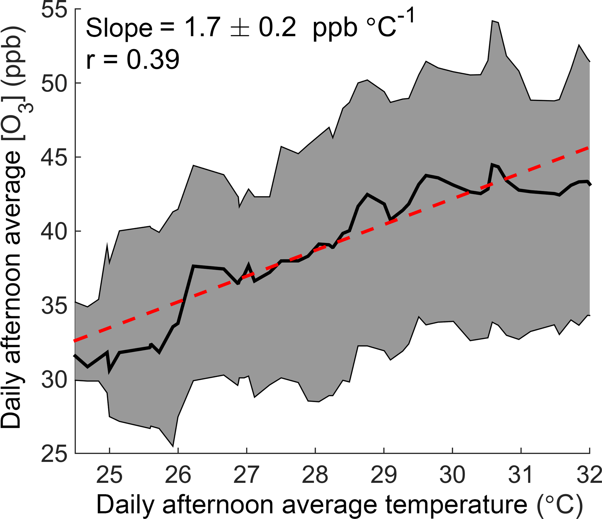
Figure 1The O3–temperature relationship in Centreville, Alabama. Daily afternoon (12:00–16:00) average ozone concentration is shown as a function of temperature over June–August 2010–2014 at the SEARCH CTR site. The black line and shaded gray region show the running median and interquartile range of ozone with temperature, respectively. The red line represents a fit to all daily data points.
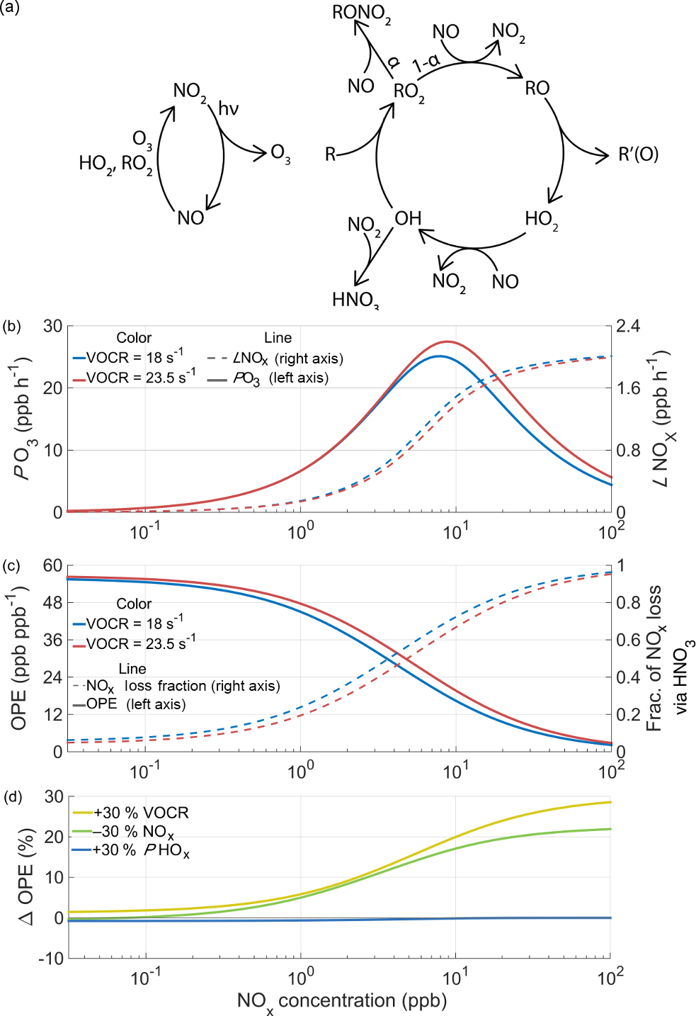
Figure 2The chemistry of ozone production and NOx loss in the troposphere. (a) Schematic of the linked NOx and HOx cycles that lead to net ozone production. (b) The calculated instantaneous O3 production rate and NOx loss rate as a function of NOx and VOCR, with fixed PHOx, η, and αeff. (c) OPE and the fraction of NOx loss that takes place via HNO3 chemistry under the same conditions as (b). (d) The percent change in ozone production efficiency caused by chemical changes as a function of NOx.
Observed O3–T relationships are caused by a combination of chemical changes to the production and loss of O3 and changes to atmospheric circulation that determine advection and mixing. To begin separating these effects, we consider the chemical production of ozone (PO3) and how it changes with temperature. Temperature-dependent changes in ozone production may be driven directly by temperature, or by another meteorological parameter that co-varies with temperature, such as solar radiation.
Ozone is produced in the troposphere when NO is converted to NO2 by reaction with HO2 or RO2 in the linked HOx and NOx cycles (Fig. 2a). HO2 and RO2 radicals are generated in the HOx cycle when a VOC reacts with OH in the presence of NOx. In one turn of the cycle, the VOC is oxidized, OH is regenerated, and two molecules of O3 are formed. The reactions that drive these catalytic cycles forward are in constant competition with reactions that remove radicals from the atmosphere, terminating the cycles. Termination can occur either through the association of two HOx radicals to form inorganic or organic peroxides, or through the association of HOx and NOx radicals to form nitric acid or an organic nitrate.
The balance between propagating and terminating reactions causes PO3 to be a non-linear function of the NOx and VOC reactivity (VOCR), as well as the production rate of HOx radicals (PHOx). The largest source of HOx radicals in the summertime is the photolysis of O3 followed by reaction with water vapor to produce OH; additional sources include the photolysis of formaldehyde and peroxides, ozonolysis of alkenes, and isomerization pathways in the oxidation of isoprene and other VOCs. To understand the response of ozone production to changes in chemistry, we use a simplified framework based on the balance of HOx radical production and loss (Farmer et al., 2011).
Under moderate or high NOx conditions, the primary loss process of HO2 and RO2 radicals is reaction with NO, and the concentration of OH radicals can be expressed as a quadratic equation. To modify this approach to work under low-NOx conditions, reactions between HOx radicals must also be included, leading to a set of four algebraic equations that can be solved numerically (details given in Appendix A). Figure 2b shows the calculated rate of ozone production as a function of NOx at two different VOC reactivities. Depending on atmospheric conditions, the ozone production rate can either be NOx-limited, where additional NOx causes PO3 to increase, or NOx-saturated, where additional NOx suppresses ozone formation.
When considering day-to-day variations, the total amount of ozone produced over the course of a day (∫PO3) is a more representative metric than the instantaneous ozone production rate. Total daily ozone production depends on all of the factors that affect PO3 as well as their diurnal evolution. In places where ozone production is NOx-limited, changes to chemistry with temperature that affect the NOx loss rate (ℒNOx) can affect ∫PO3 by changing the amount of NOx available for photochemistry later in the day (Hirsch et al., 1996).
Permanent NOx loss occurs through two primary pathways in the troposphere: the association of OH and NO2 to form HNO3, and through the chemistry of alkyl and multifunctional nitrates (ΣRONO2). These organic nitrates are formed as a minor channel of the RO2+NO reaction, with the alkyl nitrate branching ratio αi ranging from near zero for small hydrocarbons to over 0.20 for monoterpenes and long-chain alkanes (Perring et al., 2013). The overall alkyl nitrate branching ratio αeff represents the reactivity-weighted average of αi for all VOCs. While some fraction of ΣRONO2 quickly recycles NOx to the atmosphere, a significant fraction η permanently removes NOx through deposition and hydrolysis (Browne et al., 2013). Romer et al. (2016) determined that η=0.55 during SOAS and was controlled primarily by the hydrolysis of isoprene hydroxy-nitrates. Because the hydrolysis rate is set primarily by the distribution of nitrate isomers, which does not change appreciably with temperature, we assume that η is constant with temperature in this study (Hu et al., 2011; Peeters et al., 2014). Deposition is only a minor loss process for ΣRONO2, therefore any changes in the deposition rate with temperature will have, at most, a minor effect on η.
NOx also has several temporary sinks that can sequester NOx, most importantly peroxy acyl nitrate (PAN). In the summertime in the southeastern United States, the lifetime of PAN is typically 1–2 h, too short to act as a permanent sink of NOx. Past studies in forested regions have found remarkably little variation in PAN with temperature, due to compensating changes in both its production and loss (LaFranchi et al., 2009). As a result, the formation or destruction of PAN does not contribute significantly to net ozone production or NOx loss and we do not include it in these calculations.
The ozone production efficiency (OPE NOx) represents the number of ozone molecules formed per molecule of NOx consumed and directly links the ozone and NOx budgets. Because OPE accounts for changes in both PO3 and ℒNOx, the temperature response of OPE captures feedbacks in ozone production chemistry that PO3 alone does not.
As the concentration of NOx decreases and VOCR increases, the fraction of NOx loss that takes place via HNO3 chemistry decreases and the OPE increases (Fig. 2c). The relative importance of HNO3 and RONO2 chemistry determines the relationship between PO3 and ℒNOx. When HNO3 is the most important NOx loss pathway, O3 production and NOx loss occur through separate channels. O3 production occurs when OH reacts with a VOC, generating RO2 and HO2 radicals; NOx loss primarily occurs when OH reacts with NO2. Although these channels are linked by a shared dependence on OH, the relative importance of these pathways can vary. For example, under these conditions an increase in VOCR will cause NOx loss to decrease, ozone production to increase, and OPE to increase (Fig. 2b–c).
In contrast, when RONO2 chemistry dominates NOx loss, ozone production and NOx loss are intrinsically linked by their shared dependence on the RO2+NO reaction. This reaction produces O3 in its main channel and consumes NOx in the minor channel that forms organic nitrates, with the ratio between these two channels set by αeff. Under these conditions, changes to the chemistry that do not affect αeff have a minimal effect on OPE (Fig. 2d) and the OPE can be considered to be unvarying with temperature. An increase in VOCR or a decrease in NOx will affect both NOx loss and ozone production equally, because both processes are dependent on the same set of reactions. Because of this change in behavior, from variable OPE to fixed OPE, the drivers of the O3–T relationship are expected to be categorically different in areas where RONO2 chemistry dominates NOx loss. As a result, the effects that cause O3 to increase with temperature in urban and other polluted regions, where HNO3 chemistry dominates NOx loss, are unlikely to apply in areas with low concentrations of NOx and high concentrations of reactive VOCs, where RONO2 chemistry is most important. In these areas, more NOx must be oxidized in order to produce more O3.
3.1 Measurements during SOAS
The theoretical results presented in Fig. 2 can be compared to the observed behavior during SOAS (SOAS Science Team, 2013). Measurements during SOAS have been described in detail elsewhere (Feiner et al., 2016; Hidy et al., 2014; Romer et al., 2016) and are summarized below. The primary ground site for SOAS was co-located with the CTR site of the SEARCH network (32.90289∘ N, 87.24968∘ W), in a clearing surrounded by a dense mixed forest (Hansen et al., 2003). Direct anthropogenic emissions of NOx near this site are estimated to be low and predominantly from mobile sources (Hidy et al., 2014). Figure S1 shows the location of the CTR site relative to major population centers in the region. Measurements taken as part of the SEARCH network were located on a 10 m tower approximately 100 m away from the forest edge, while the other measurements from the SOAS campaign used in this analysis were located on a 20 m walk-up tower at the edge of the forest. Species measured on both the SOAS walk-up tower and the SEARCH platform were well correlated with each other, indicating that similar air masses were sampled at both locations.
Several chemical and meteorological measurements used in this study, including NOx, O3, total reactive nitrogen (NOy), and temperature, were collected by Atmospheric Research and Analysis (ARA) as part of SEARCH (Hidy et al., 2014). NO was measured using the chemiluminescent reaction of NO with excess ozone. NO2 was measured based on the same principle, using blue LED photolysis to convert NO2 to NO. The photolytic conversion of NO2 to NO is nearly 100 % efficient and does not affect higher oxides of nitrogen (Ryerson et al., 2000). Ozone was measured using a commercially available ozone analyzer (Thermo-Scientific 49i).
During the SOAS campaign, NO2, total peroxy nitrates (ΣPNs), and total alkyl and multifunctional nitrates (ΣRONO2) were measured via thermal dissociation laser-induced fluorescence, as described by Day et al. (2002). An NO chemiluminescence instrument located on the walk-up tower provided additional measurements of NO co-located with the other SOAS measurements (Min et al., 2014).
HOx radicals were measured with the Penn State Ground-based Tropospheric Hydrogen Oxides Sensor (GTHOS), which uses laser-induced fluorescence to measure OH (Faloona et al., 2004). HO2 was also measured in this instrument by adding NO to convert HO2 to OH. C3F6 was periodically added to the sampling inlet to quantify the interference from internally generated OH (Feiner et al., 2016). Measurements of total OH reactivity (OHR ≡ inverse OH lifetime) were made by sampling ambient air, injecting OH, and letting the mixture react for a variable period of time. The slope of the OH signal vs. reaction time provides a top-down measure of OHR (Mao et al., 2009).

Figure 3Observed dependence of daily ∫PO3 (a), ∫ℒO3 (b), and ∫ℒNOx (c) on daily afternoon average temperature during SOAS. Each point shows the afternoon average temperature and integrated production or loss for a single day. Black lines show a least squares fit to all points; shaded areas show the 90 % confidence limits of the fit calculated via bootstrap sampling.
A wide range of VOCs were measured during SOAS using gas chromatography-mass spectrometry (GC-MS). Samples were collected in a liquid-nitrogen cooled trap for five minutes, then transferred by heating onto an analytical column, and detected using an electron-impact quadrupole mass-spectrometer (Gilman et al., 2010). This system is able to quantify a wide range of compounds including alkanes, alkenes, aromatics, isoprene, and multiple monoterpenes at a time resolution of 30 min. Methyl vinyl ketone (MVK) and methacrolein (MACR) were measured individually by GC-MS and their sum was also measured using a proton transfer reaction mass spectrometer (PTR-MS) (Kaser et al., 2013). The calculated rates of ozone production and NOx loss do not change significantly depending on which measurement is used.
3.2 Calculation of ∫PO3 and effects of temperature
During the SOAS campaign, afternoon concentrations of NOx averaged 0.3 ppb and concentrations of isoprene 5.5 ppb (Fig. S2). ΣRONO2 chemistry was responsible for over three-quarters of the permanent NOx loss (Romer et al., 2016). Daily average afternoon (12:00–16:00) ozone concentrations increased with daily average afternoon temperature during SOAS (2.3 ± 1 ppb ∘C−1). This trend is greater than the long-term trend reported by the SEARCH network, but the difference is not statistically significant.
Measurements of NO, NO2, OH, HO2, and a wide range of VOCs (Table S1) were used to calculate the steady-state concentrations of RO2 radicals using the Master Chemical Mechanism v3.3.1, run in a MATLAB framework (Jenkin et al., 2015; Wolfe et al., 2016). Before 24 June, HO2 measurements are not available and steady-state concentrations of both HO2 and RO2 were calculated. Input species were taken to 30 min averages, and the model was run until radical concentrations reached steady state. Top-down measurements of OHR were used to include the contribution to ozone production from unmeasured VOCs.
To understand the day-to-day variation of ozone chemistry, the calculated ozone production rate was integrated from 06:00 to 16:00 for each of the 24 days during the campaign period with greater than 75 % data coverage of all input species. When plotted against daily average afternoon temperature, ∫PO3 is seen to increase strongly with temperature (2.3 ± 0.6 ppb ∘C−1, Fig. 3a). The change in ∫PO3 with temperature demonstrates that local chemistry is an important contributor to the observed O3–T relationship; however, the observed O3–T trend also includes the effects of chemical loss, advection, entrainment, and multi-day buildup on overall O3 concentration (Baumann et al., 2000).
While elevated temperatures are associated with enhanced production of ozone, they are also associated with increased chemical loss. The chemical loss of ozone occurs via three main pathways in this region: photolysis followed by reaction with H2O, reaction with HO2, and reaction with VOCs (Frost et al., 1998). The loss of O3 was calculated for each of these pathways, and then integrated over the course of the day to determine total daily ozone loss (∫ℒO3). Chemical loss of ozone is found to increase with temperature (1.1 ± 0.3 ppb ∘C−1, Fig. 3b), but much less than the chemical production.
The difference between the trend in the net chemical production and loss of O3 and the trend in ozone concentration gives a rough estimate of how non-chemical processes contribute to the ozone–temperature relationship. We calculate that non-chemical processes cause O3 to increase by 1 ± 1.2 ppb ∘C−1. This approach does not take into account the interactions between chemical and non-chemical effects, such as how changes to advection and mixing may impact concentrations of VOCs, NOx, and other reactants. Although the large uncertainty does not allow for quantitative analysis, qualitatively, chemical and non-chemical processes are both found to be important contributors to the ozone–temperature relationship. Other approaches, such as chemical transport models, that can more directly investigate and control specific physical processes are likely to be better suited to calculating the contribution of non-chemical processes to the ozone–temperature relationship (Fu et al., 2015).
Using the same calculated radical concentrations, the rate of NOx loss was calculated as the rate of direct HNO3 production plus the fraction η of alkyl nitrate production that leads to permanent NOx loss. Figure 3c shows the increase in ∫ℒNOx with temperature for the SOAS campaign (0.05 ± 0.01 ppb ∘C−1). As expected from the importance of RONO2 chemistry to NOx loss, ∫ℒNOx and ∫PO3 are tightly correlated (r2=0.90), and OPE is high (OPE average 45 ± 3 ppb ppb−1) and is effectively constant with temperature (calculated trend 0.2 ± 0.6 ∘C−1). Therefore, the increase in ∫PO3 with temperature is not caused by more efficient production of ozone while the same amount of NOx is consumed.
OPE can also be estimated from the ratio of odd oxygen (Ox ) to NOx oxidation products (NO) (Trainer et al., 1993). The afternoon ratio of Ox to NOz during SOAS varied from 43 to 67 (interquartile range), slightly higher than the average ratio of ∫PO3 to ∫ℒNOx. However, since the Ox to NOz ratio includes the effects of chemical loss and transport, which the ratio of ∫PO3 to ∫ℒNOx does not, these two values are not expected to be equivalent, particularly in non-polluted areas.
The trend in ∫PO3 with temperature is robust and extends beyond the short temporal window of the SOAS campaign. Although long-term measurements of HOx and VOCs are not available, the ozone production rate can be estimated from SEARCH measurements using the deviation of NO and NO2 from photostationary state (Eq. 1) (Baumann et al., 2000; Pusede et al., 2015).
The NO2 photolysis rate was parameterized as a quadratic function of total solar radiation (Trebs et al., 2009). Using this method and scaling the result to match the values calculated using steady-state RO2 concentrations during SOAS, we find that ∫PO3 increased by 2.3 ± 0.8 ppb ∘C−1 during June–August 2010–2014 (Fig. S3). Without scaling, the long-term trend in ∫PO3 with temperature is 4.0 ± 0.5 ppb ∘C−1. Based on the long-term SEARCH record, we do not find evidence that the relationship between temperature and ozone concentration or ozone production changes significantly at the highest temperatures (the top 5 % of observations). This agrees broadly with Shen et al. (2016), who found ozone suppression at extreme temperatures to be uncommon in the southeastern United States.
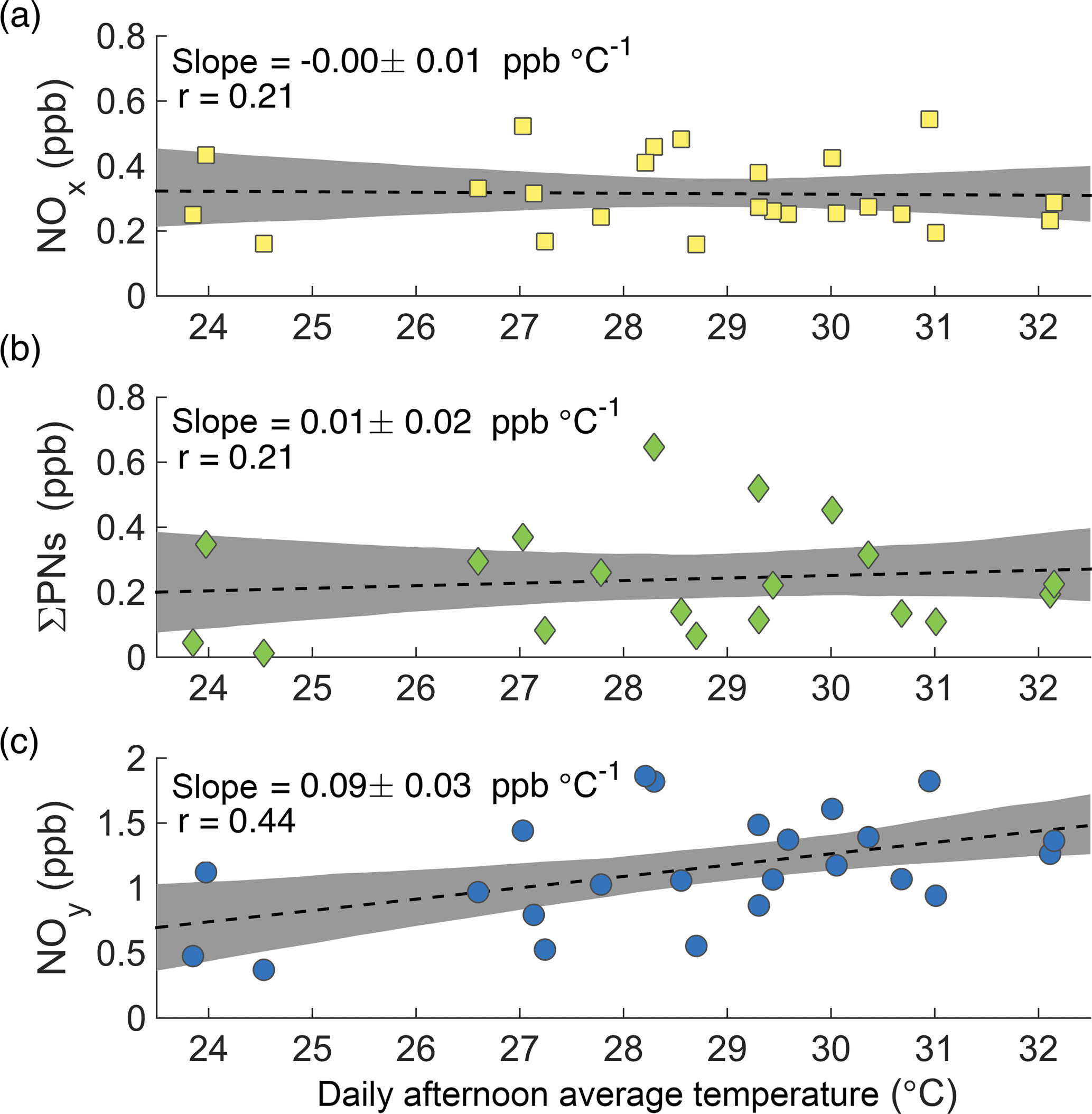
Figure 4Afternoon average concentrations of NOx (a), ΣPNs (b), and NOy (c) at the CTR site as a function of daily average afternoon temperature during SOAS.
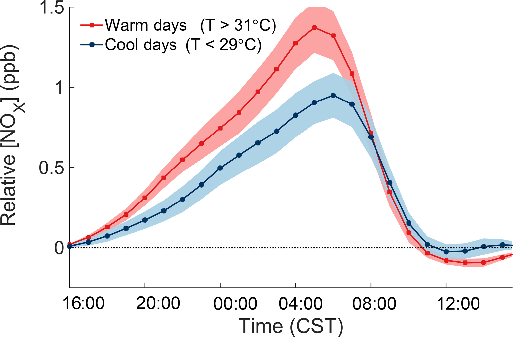
Figure 5Concentrations of NOx relative to their concentration at 16:00 the day before over June–August 2010–2014 at the CTR site. The thick lines and shaded areas show the hourly mean and 90 % confidence interval of the mean for cool and warm days.
While the increase in ozone production is accompanied by an observed increase in ozone concentration, the increase in NOx loss is not accompanied by a significant decrease in NOx concentration ( ppb ∘C−1, Fig. 4a). For this to occur, NOx must have a source that increases with temperature to compensate for its increased loss. One possible explanation is that the increased thermal decomposition rate of peroxy nitrates (ΣPNs) causes less NOx to be sequestered in these short-term reservoirs. This is not the case during SOAS. The increased decomposition rate of peroxy nitrates is counteracted by an increase in their production rate, such that the average concentration of total peroxy nitrates shows no decrease with temperature (Fig. 4b).
More generally, increased transformations from NOx oxidation products back into NOx cannot explain the observations. The concentration of NOy increases significantly with temperature (Fig. 4c). Because NOy includes NOx as well as all of its reservoirs and sinks, changes in the transformation rates between NOx and its oxidation products cannot explain the increase of NOy with temperature. There must be a source of NOy, not just of NOx, that increases with temperature.
Data from the SEARCH network indicate that the increase in NOy with temperature observed during SOAS is primarily a local effect. Measurements from June to August 2010–2014 show a consistent increase of NOy with temperature at the two rural monitoring sites in the network, but total NOy decreases with temperature at the four urban and suburban sites (Table S2). The increase in NOy with temperature cannot therefore be explained by regional meteorological effects, since those would lead to similar relationships between NOy and temperature across the southeastern United States.
Measurements at night and in the early morning, before significant photochemistry has occurred, show a strong temperature-dependent increase of NOx over the course of the night. Because surface wind speeds are low at night and the increase in NOx during the night is not accompanied by large increases in NOx oxidation products, the increase in NOx must be caused by emissions local to the CTR site.
The consistent increase of NOx over the course of the night can be used to quantitatively measure the local NOx emissions rate. Figure 5 shows the temperature-dependent increase of NOx relative to the concentration of NOx at 16:00 the day before, separating the effects of the previous day from the nighttime increase. Measurements from June to August 2010–2014 from the CTR SEARCH network site are used to obtain more representative statistics. The average rate of NOx increase during the night is 0.095 ppb h−1. To account for the chemical removal of NOx, the cumulative loss of NOx during the night was added to the observations. During SOAS, the nighttime loss of NOx occurred almost exclusively through the reaction of NO2 with O3 to form NO3, which then reacted with a VOC to form an organic nitrate (Ayres et al., 2015). N2O5 chemistry made a negligible contribution to total NOx loss. The loss rate of NOx during the night was therefore calculated as the rate of reaction of NO2 with O3. In this form, the rate of increase of the adjusted NOx concentrations () is equal to the local NOx emission rate. The emission rate of NOx and its temperature dependence were calculated by a linear regression following the form of Eq. (2), where the adjusted concentration of NOx depends both on time (H is hours after 16:00) and temperature (T).
In this regression, the fitted parameter α represents the increase of NOx emissions with temperature and the average value of αT+β provides an estimated NOx emission rate.
Because emissions are localized to the surface, the effective depth of the nighttime boundary layer must also be accounted for, which we estimate to be 150 m. This agrees well with the derived mixing heights from daily 05:00 sonde launches at the Birmingham (BHM) airport (Durre and Yin, 2008) and past estimates of the nocturnal boundary layer height (Liu and Liang, 2010; VandenBoer et al., 2013), while it is significantly lower than the average ceilometer-reported 05:00 boundary layer height of 400 m during SOAS (Fig. S4).
After accounting for these factors, the NOx emissions rate is calculated to be 7.4 ppt m s−1 or 4.2 ng N . Based on the change in slope with temperature, the emissions rate is estimated to increase by 0.4 ppt m −1. The rise in NOx emissions with temperature over 24 h agrees to within the uncertainty with the increase of daily ∫ℒNOx with temperature, sufficient to explain why afternoon NOx concentrations are not observed to decrease with temperature even as their loss rate increases.
The inferred local NOx source bears all the hallmarks of soil microbial emissions (). Soil microbes emit NOx as a byproduct of both nitrification and denitrification, and the rate of NOx emissions strongly correlates with microbial activity in soil (Pilegaard, 2013). The inferred NOx source is active during day and night, increases strongly with temperature, and is present in a rural area with low anthropogenic emissions. The only plausible source of NOx that matches all of these constraints is soil microbial emissions near the SOAS site. Soil NOx emissions also depend on the water content and nitrogen availability, neither of which is generally limiting in the southeastern United States (Hickman et al., 2010). The most likely anthropogenic sources of NOx at this location are mobile sources, which are not thought to change significantly with temperature (Singh and Sloan, 2006) , and therefore cannot explain the results of Fig. 5.
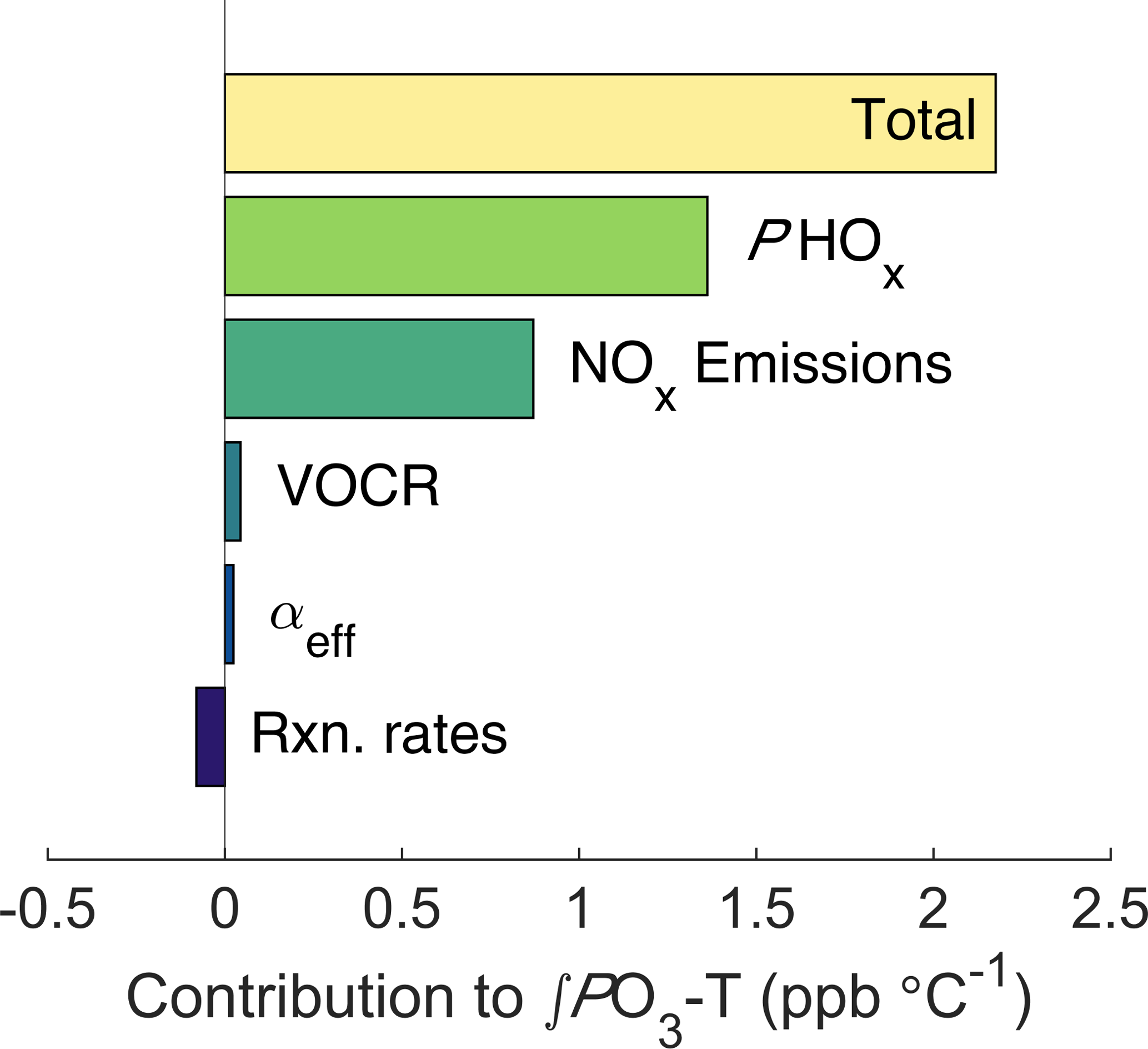
Figure 6Decomposed effects of ozone and temperature. The top bar shows the model-calculated ∫PO3-T trend, all other bars show how the ∫PO3-T slope changes when the temperature dependence of each factor is removed.
To calculate how the increase in NOx emissions affects ozone production, we use the same chemical framework from Fig. 2. For each half-hour period the average value of the input parameters and their temperature dependence during the SOAS campaign were calculated (Fig. S5). The diurnal cycle and trend with temperature of all model inputs were then used to calculate total daily ozone production as a function of temperature (Fig. S6). By altering whether the temperature dependence for each parameter is included, the overall trend in ∫PO3 can be decomposed into individual components (Fig. 6). The effect of increased NOx emissions was calculated by fixing the trend in NOx with temperature to match the trend in ∫ℒNOx. We find that the increase of NOx emissions with temperature accounts for 40 % of the increase in ∫PO3 with temperature, or approximately 0.9 ppb ∘C−1. The other 60 % is primarily caused by the increase of PHOx with temperature. The increase in PHOx with temperature is most likely caused by changes in solar radiation, which is well correlated with the total PHOx rate (Fig. S7a) and increases strongly with temperature. In contrast, water vapor is not correlated with total PHOx (Fig. S7b). Although VOCR increases strongly with temperature, the RONO2-dominated NOx chemistry causes neither the ozone production rate nor the NOx loss rate to be sensitive to this increase, leading to the minimal effect of VOCR on ∫PO3.
Changes in NOx emissions with temperature have an outsized effect when considering the impacts of ozone on human health and climate. At the CTR site and other areas where OPE does not vary with temperature, the total amount of ozone produced on weekly or monthly timescales is directly proportional to the amount of available NOx. While faster oxidation on hotter days causes more ozone to be produced, without changes in NOx emissions there would be an associated decrease in ozone production on subsequent days, because the NOx necessary for ozone production would be depleted. In contrast, increased NOx emissions can cause weekly or monthly average ozone concentrations to increase with temperature. Change in long-term average ozone concentrations is often more important to the ozone climate feedback and human health than day-to-day variation. The mechanisms described here are likely to be active in all areas with low concentrations of NOx and high concentrations of reactive VOCs. Only regions where RONO2 chemistry is the dominant pathway for NOx loss have effectively constant OPE with temperature, but the effect of soil NOx emissions on ozone production is widespread.
Past direct measurements of soil NOx using soil chambers have found enormous variability, both between sites and within different plots in the same field. Pilegaard et al. (2006) found variability of a factor of over 100 between soil NOx emissions in different European forests. Within the southeastern United States, direct measurements at forested sites have reported emissions rates ranging from 0.1 to 10 ng N (Hickman et al., 2010; Thornton et al., 1997; Williams and Fehsenfeld, 1991). Besides temperature, the most important variables affecting soil NOx emissions are typically nitrogen availability and soil water content, as well as plant cover and soil pH (Pilegaard, 2013). In very wet environments, soil microbes typically emit N2O or N2 instead of NOx, and in arid environments soil emissions of HONO can be equal to or larger than soil NOx emissions (Oswald et al., 2013). Although conditions at the CTR site are too wet and acidic for soil HONO emissions to be significant, in environments where soil HONO emissions are large, they would likely have an even greater effect on ozone production by acting as a source of both NOx and HOx radicals.
The variability between sites and the interaction between several biotic and abiotic factors make it difficult to apply regional or model estimates of soil NOx emissions to a particular location. Our approach from this study, using observations of the nighttime atmosphere to determine the NOx emissions rate, helps span the gap between soil chambers and the regional atmosphere. Although soil NOx emissions depend on several environmental factors, process-driven models predict that the response of soil NOx emissions to global warming will be driven primarily by the increase in temperature (Kesik et al., 2006).
While soil NOx emissions have been known and studied for decades, the impact of soil NOx emissions on ozone from non-agricultural regions was often found to be insignificant compared to anthropogenic sources (Davidson et al., 1998). Years of declining anthropogenic NOx emissions in the United States and recent higher estimates for forest soil NOx emissions (Hickman et al., 2010) mean that this is no longer the case. Non-agricultural soil NOx emissions may now account for nearly a third of total NOx emissions in the summertime in the southeastern United States (Travis et al., 2016), and have significant effects on regional ozone production.
The rise in ozone production caused by increased NOx emissions on hotter days established here suggests that the relationship between ozone and temperature will be positive under a wider range of conditions than previously thought. This includes 1. the pre-industrial atmosphere, 2. present day rural continental locations, and 3. future scenarios with dramatically reduced anthropogenic NOx emissions.
-
In pre-industrial times, semi-quantitative measurements of ozone show significantly lower concentrations of ozone than are currently observed in rural and remote regions or generally predicted by global models (Cooper et al., 2014). While alkyl nitrate chemistry establishes an upper limit to the ozone production efficiency under low-NOx conditions, the significant contribution of to ozone production makes reconciling the semi-quantitative measurements with model predictions more difficult and suggests that natural emissions of NOx in pre-industrial models may be over-estimated (Mickley et al., 2001).
-
In the present day, effective ozone regulation, especially on hot days, requires taking the effect of into account. Because these emissions are distributed over broad areas and are not directly anthropogenic, they present additional challenges to air quality management. Indirect approaches, such as changes to fertilizer application practices, have the potential to significantly reduce from agricultural regions (Oikawa et al., 2015). Decreases in direct anthropogenic NOx emissions may also lead to a decrease in by reducing the amount of nitrogen available to the ecosystem (Pilegaard, 2013).
-
In the future, because soil NOx emissions lead to the formation of ozone, itself an important greenhouse gas, the increase of soil NOx emissions with temperature represents a positive climate feedback and an additional link between changes to the nitrogen cycle and the environment. The effects of increased ozone pollution to plants, including reduced photosynthesis and slower growth, have the potential to alter the carbon cycle on a regional scale (Booker et al., 2009; Heagle, 1989). Soil NOx emissions therefore represent an additional link between the nitrogen and carbon cycles that should be included when considering the consequences of a warming world.
Measurements from the SOAS campaign are available at https://esrl.noaa.gov/csd/groups/csd7/measurements/2013senex/Ground/DataDownload (SOAS Science Team, 2013).
Analytical PO3 model
To conceptually understand O3 production and NOx loss, we use a simplified framework similar to that described by Farmer et al. (2011). This framework uses fixed values of total organic reactivity (VOCR), alkyl nitrate branching ratio α and loss efficiency η, NOx, and HOx radical production rate (PHOx).
Since HOx radicals are highly reactive, it is a valid assumption under nearly all NOx concentrations that HOx radicals are in steady state and that PHOx is equal to the gross HOx loss rate (Eq. A1).
Individual HOx radicals (OH, HO2, and RO2) can also be assumed to be in steady state, such that their production and loss are equal. Under low-NOx conditions, the reactions that initiate and terminate the HOx cycle must be included, as well as the cycling rate. We further constrain the model by requiring that the concentration of HO2 and RO2 radicals be equal. This constraint is satisfied by introducing an additional parameter c which allows PHOx to produce both HO2 and OH radicals in a varying ratio. These constraints provide a system of four equations that can be solved numerically (Eqs. A2–A5).
For the calculations in Fig. 2, the values of VOCR, α,
and PHOx were fixed at 18 s−1, 0.06, and 1.15×10⁷ molec cm−3 s−1. Rate constants are taken from the
IUPAC chemical kinetics database, assuming that all RO2 radicals
react with the kinetics of CH3CH2O2
(Atkinson et al., 2006). The system of equations was solved
numerically using the vpasolve function in MATLAB, subject to the
constraints that [OH],[HO2], and [RO2] are positive
and c is between 0 and 1.
The resulting concentrations of HOx radicals can be used to calculate the rates of ozone production and NOx loss using Eqs. (A6)–(A9).
Decomposition of the O3-temperature relationship
The simplified HOx model described above was used to decompose the contribution of different parameters to the increase of ∫PO3 with temperature. Peroxy nitrates are not included in this model, but because there is no significant trend in ΣPNs with temperature their absence does not affect the results. To validate that this model gave accurate ∫PO3 results, it was first run using inputs based on measured values for each half-hour period:
-
Model inputs of NOx were taken directly from measurements of NO and NO2
-
VOCR was calculated as the measured OHR minus the reactivity of species that do not form RO2 radicals (e.g., CO, NO2)
-
PHOx was calculated as equal to the measured rate of HOx loss, using Eq. (A1) and measured HOx radical concentrations
-
αeff was calculated as the reactivity-weighted average of αi for all measured VOCs.
The comparison of ∫PO3 calculated from the full data set and that from the steady-state HOx model is shown in Fig. S6a. The two calculations are well-correlated with a slope close to one, showing that the steady-state HOx model can accurately reproduce ozone production at this location.
To use this model to explore how ozone production changes with temperature, the diurnal cycle and trend in temperature of each of these inputs was calculated. Because the response to temperature is different at different times of day, the trend with temperature was calculated independently for each half-hour bin, and is shown in Fig. S5. These trends were used to construct temperature-dependent diurnal cycles of each of the parameters, which were then used as inputs to the model at a range of daily average afternoon temperatures from 24 to 32 ∘C. Figure S6b shows that ∫PO3 calculated this way has a very similar trend with temperature as that using the full data set, although it cannot capture day-to-day variability not caused by temperature. The nonlinear shape of the trend with temperature is caused primarily by the imposed exponential increase of PHOx with temperature. Using a linear or quadratic increase of PHOx with temperature changes the shape of the increase but does not significantly affect the overall ∫PO3-T slope.
The authors declare that they have no conflict of interest.
The supplement related to this article is available online at: https://doi.org/10.5194/acp-18-2601-2018-supplement.
Financial and logistical support for SOAS was provided by the NSF, the Earth
Observing Laboratory at the National Center for Atmospheric Research
(operated by NSF), the personnel at Atmospheric Research and Analysis, and
the Electric Power Research Institute. We are grateful to Kevin Olson and Li Zhang for assistance with measurements during SOAS. Funding for the SEARCH
network was provided by Southern Company Services and the Electric Power
Research Institute. The Berkeley authors acknowledge the support of the NOAA
Office of Global Programs grant NA13OAR4310067 and NSF grant
AGS-1352972.
Edited by: Andreas Hofzumahaus
Reviewed by: two anonymous referees
Atkinson, R., Baulch, D. L., Cox, R. A., Crowley, J. N., Hampson, R. F., Hynes, R. G., Jenkin, M. E., Rossi, M. J., Troe, J., and IUPAC Subcommittee: Evaluated kinetic and photochemical data for atmospheric chemistry: Volume II – gas phase reactions of organic species, Atmos. Chem. Phys., 6, 3625–4055, https://doi.org/10.5194/acp-6-3625-2006, 2006. a
Atkinson, R. W., Yu, D., Armstrong, B. G., Pattenden, S., Wilkinson, P., Doherty, R. M., Heal, M. R., and Anderson, H. R.: Concentration–Response Function for Ozone and Daily Mortality: Results from Five Urban and Five Rural U.K. Populations, Environ. Health Persp., 120, 1411–1417, 2012. a
Ayres, B. R., Allen, H. M., Draper, D. C., Brown, S. S., Wild, R. J., Jimenez, J. L., Day, D. A., Campuzano-Jost, P., Hu, W., de Gouw, J., Koss, A., Cohen, R. C., Duffey, K. C., Romer, P., Baumann, K., Edgerton, E., Takahama, S., Thornton, J. A., Lee, B. H., Lopez-Hilfiker, F. D., Mohr, C., Wennberg, P. O., Nguyen, T. B., Teng, A., Goldstein, A. H., Olson, K., and Fry, J. L.: Organic nitrate aerosol formation via NO3 + biogenic volatile organic compounds in the southeastern United States, Atmos. Chem. Phys., 15, 13377–13392, https://doi.org/10.5194/acp-15-13377-2015, 2015. a
Barnes, E. A. and Fiore, A. M.: Surface ozone variability and the jet position: Implications for projecting future air quality, Geophys. Res. Lett., 40, 2839–2844, https://doi.org/10.1002/grl.50411, 2013. a
Baumann, K., Williams, E. J., Angevine, W. M., Roberts, J. M., Norton, R. B., Frost, G. J., Fehsenfeld, F. C., Springston, S. R., Bertman, S. B., and Hartsell, B.: Ozone production and transport near Nashville, Tennessee: Results from the 1994 study at New Hendersonville, J. Geophys. Res., 105, 9137–9153, https://doi.org/10.1029/1999JD901017, 2000. a, b
Berlin, S. R., Langford, A. O., Estes, M., Dong, M., and Parrish, D. D.: Magnitude, Decadal Changes, and Impact of Regional Background Ozone Transported into the Greater Houston, Texas, Area, Environ. Sci. Technol., 47, 13985–13992, https://doi.org/10.1021/es4037644, 2013. a
Booker, F., Muntifering, R., McGrath, M., Burkey, K., Decoteau, D., Fiscus, E., Manning, W., Krupa, S., Chappelka, A., and Grantz, D.: The Ozone Component of Global Change: Potential Effects on Agricultural and Horticultural Plant Yield, Product Quality and Interactions with Invasive Species, J. Integr. Plant Biol., 51, 337–351, https://doi.org/10.1111/j.1744-7909.2008.00805.x, 2009. a, b, c
Browne, E. C., Min, K.-E., Wooldridge, P. J., Apel, E., Blake, D. R., Brune, W. H., Cantrell, C. A., Cubison, M. J., Diskin, G. S., Jimenez, J. L., Weinheimer, A. J., Wennberg, P. O., Wisthaler, A., and Cohen, R. C.: Observations of total RONO2 over the boreal forest: NOx sinks and HNO3 sources, Atmos. Chem. Phys., 13, 4543–4562, https://doi.org/10.5194/acp-13-4543-2013, 2013. a
Cooper, O. R., Gao, R.-S., Tarasick, D., Leblanc, T., and Sweeney, C.: Long-term ozone trends at rural ozone monitoring sites across the United States, 1990–2010, J. Geophys. Res. Atmos., 117, D22307, https://doi.org/10.1029/2012JD018261, 2012. a
Cooper, O. R., Parrish, D. D., Ziemke, J., Balashov, N. V., Cupeiro, M., Galbally, I. E., Gilge, S., Horowitz, L., Jensen, N. R., Lamarque, J.-F., Naik, V., Oltmans, S. J., Schwab, J., Shindell, D. T., Thompson, A. M., Thouret, V., Wang, Y., and Zbinden, R. M.: Global distribution and trends of tropospheric ozone: An observation-based review, Elem. Sci. Anth., 2, 000029, https://doi.org/10.12952/journal.elementa.000029, 2014. a
Davidson, E. A., Potter, C. S., Schlesinger, P., and Klooster, S. A.: Model estimates of regional nitric oxide emissions from soils of the Southeastern United States, Ecol. Appl., 8, 748–759, https://doi.org/10.1890/1051-0761(1998)008[0748:MEORNO]2.0.CO;2, 1998. a
Day, D. A., Wooldridge, P. J., Dillon, M. B., Thornton, J. A., and Cohen, R. C.: A thermal dissociation laser-induced fluorescence instrument for in situ detection of NO2, peroxy nitrates, alkyl nitrates, and HNO3, J. Geophys. Res., 107, 4046, https://doi.org/10.1029/2001JD000779, 2002. a
Durre, I. and Yin, X.: Enhanced radiosonde data for studies of vertical structure, B. Am. Meteorol. Soc., 89, 1257–1262, https://doi.org/10.1175/2008BAMS2603.1, 2008. a
Faloona, I. C., Tan, D., Lesher, R. L., Hazen, N. L., Frame, C. L., Simpas, J. B., Harder, H., Martinez, M., Di Carlo, P., Ren, X., and Brune, W. H.: A Laser-induced Fluorescence Instrument for Detecting Tropospheric OH and HO2: Characteristics and Calibration, J. Atmos. Chem., 47, 139–167, https://doi.org/10.1023/B:JOCH.0000021036.53185.0e, 2004. a
Farmer, D. K., Perring, A. E., Wooldridge, P. J., Blake, D. R., Baker, A., Meinardi, S., Huey, L. G., Tanner, D., Vargas, O., and Cohen, R. C.: Impact of organic nitrates on urban ozone production, Atmos. Chem. Phys., 11, 4085–4094, https://doi.org/10.5194/acp-11-4085-2011, 2011. a, b
Feiner, P. A., Brune, W. H., Miller, D. O., Zhang, L., Cohen, R. C., Romer, P. S., Goldstein, A. H., Keutsch, F. N., Skog, K. M., Wennberg, P. O., Nguyen, T. B., Teng, A. P., DeGouw, J., Koss, A., Wild, R. J., Brown, S. S., Guenther, A., Edgerton, E., Baumann, K., and Fry, J. L.: Testing Atmospheric Oxidation in an Alabama Forest, J. Atmos. Sci., 73, 4699–4710, https://doi.org/10.1175/JAS-D-16-0044.1, 2016. a, b
Frost, G. J., Trainer, M., Allwine, G., Buhr, M. P., Calvert, J. G., Cantrell, C. A., Fehsenfeld, F. C., Goldan, P. D., Herwehe, J., Hübler, G., Kuster, W. C., Martin, R., McMillen, R. T., Montzka, S. A., Norton, R. B., Parrish, D. D., Ridley, B. A., Shetter, R. E., Walega, J. G., Watkins, B. A., Westberg, H. H., and Williams, E. J.: Photochemical ozone production in the rural southeastern United States during the 1990 Rural Oxidants in the Southern Environment (ROSE) program, J. Geophys. Res., 103, 22491–22508, https://doi.org/10.1029/98JD00881, 1998. a
Fu, T.-M., Zheng, Y., Paulot, F., Mao, J., and Yantosca, R. M.: Positive but variable sensitivity of August surface ozone to large-scale warming in the southeast United States, Nat. Clim. Change, 5, 454–458, https://doi.org/10.1038/nclimate2567, 2015. a
Gilman, J. B., Burkhart, J. F., Lerner, B. M., Williams, E. J., Kuster, W. C., Goldan, P. D., Murphy, P. C., Warneke, C., Fowler, C., Montzka, S. A., Miller, B. R., Miller, L., Oltmans, S. J., Ryerson, T. B., Cooper, O. R., Stohl, A., and de Gouw, J. A.: Ozone variability and halogen oxidation within the Arctic and sub-Arctic springtime boundary layer, Atmos. Chem. Phys., 10, 10223–10236, https://doi.org/10.5194/acp-10-10223-2010, 2010. a
Hansen, D. A., Edgerton, E. S., Hartsell, B. E., Jansen, J. J., Kandasamy, N., Hidy, G. M., and Blanchard, C. L.: The Southeastern Aerosol Research and Characterization Study: Part 1 – Overview, J. Air Waste Manage., 53, 1460–1471, https://doi.org/10.1080/10473289.2003.10466318, 2003. a
Heagle, A. S.: Ozone and Crop Yield, Annu. Rev. Phytopathol., 27, 397–423, https://doi.org/10.1146/annurev.py.27.090189.002145, 1989. a
Hickman, J. E., Wu, S., Mickley, L. J., and Lerdau, M. T.: Kudzu (Pueraria montana) invasion doubles emissions of nitric oxide and increases ozone pollution, Proc. Natl. Acad. Sci. USA, 107, 10115–10119, https://doi.org/10.1073/pnas.0912279107, 2010. a, b, c
Hidy, G. M., Blanchard, C. L., Baumann, K., Edgerton, E., Tanenbaum, S., Shaw, S., Knipping, E., Tombach, I., Jansen, J., and Walters, J.: Chemical climatology of the southeastern United States, 1999–2013, Atmos. Chem. Phys., 14, 11893–11914, https://doi.org/10.5194/acp-14-11893-2014, 2014. a, b, c
Hirsch, A. I., Munger, J. W., Jacob, D. J., Horowitz, L. W., and Goldstein, A. H.: Seasonal variation of the ozone production efficiency per unit NOx at Harvard Forest, Massachusetts, J. Geophys. Res., 101, 12659–12666, https://doi.org/10.1029/96JD00557, 1996. a
Hu, K. S., Darer, A. I., and Elrod, M. J.: Thermodynamics and kinetics of the hydrolysis of atmospherically relevant organonitrates and organosulfates, Atmos. Chem. Phys., 11, 8307–8320, https://doi.org/10.5194/acp-11-8307-2011, 2011. a
Ito, K., De Leon, S. F., and Lippmann, M.: Associations Between Ozone and Daily Mortality: Analysis and Meta-Analysis, Epidemiology, 16, 446–457, https://doi.org/10.1097/01.ede.0000165821.90114.7f, 2005. a
Jacob, D. J. and Winner, D. A.: Effect of climate change on air quality, Atmos. Environ., 43, 51–63, https://doi.org/10.1016/j.atmosenv.2008.09.051, 2009. a
Jacob, D. J., Logan, J. A., Gardner, G. M., Yevich, R. M., Spivakovsky, C. M., Wofsy, S. C., Sillman, S., and Prather, M. J.: Factors regulating ozone over the United States and its export to the global atmosphere, J. Geophys. Res., 98, 14817–14826, https://doi.org/10.1029/98JD01224, 1993. a
Jenkin, M. E., Young, J. C., and Rickard, A. R.: The MCM v3.3.1 degradation scheme for isoprene, Atmos. Chem. Phys., 15, 11433–11459, https://doi.org/10.5194/acp-15-11433-2015, 2015. a
Kaser, L., Karl, T., Schnitzhofer, R., Graus, M., Herdlinger-Blatt, I. S., DiGangi, J. P., Sive, B., Turnipseed, A., Hornbrook, R. S., Zheng, W., Flocke, F. M., Guenther, A., Keutsch, F. N., Apel, E., and Hansel, A.: Comparison of different real time VOC measurement techniques in a ponderosa pine forest, Atmos. Chem. Phys., 13, 2893–2906, https://doi.org/10.5194/acp-13-2893-2013, 2013. a
Kesik, M., Brüggemann, N., Forkel, R., Kiese, R., Knoche, R., Li, C., Seufert, G., Simpson, D., and Butterbach-Bahl, K.: Future scenarios of N2O and NO emissions from European forest soils, J. Geophys. Res., 111, G02018, https://doi.org/10.1029/2005JG000115, 2006. a
LaFranchi, B. W., Wolfe, G. M., Thornton, J. A., Harrold, S. A., Browne, E. C., Min, K. E., Wooldridge, P. J., Gilman, J. B., Kuster, W. C., Goldan, P. D., de Gouw, J. A., McKay, M., Goldstein, A. H., Ren, X., Mao, J., and Cohen, R. C.: Closing the peroxy acetyl nitrate budget: observations of acyl peroxy nitrates (PAN, PPN, and MPAN) during BEARPEX 2007, Atmos. Chem. Phys., 9, 7623–7641, https://doi.org/10.5194/acp-9-7623-2009, 2009. a
Liu, S. and Liang, X.-Z.: Observed Diurnal Cycle Climatology of Planetary Boundary Layer Height, J. Climate, 23, 5790–5809, https://doi.org/10.1175/2010JCLI3552.1, 2010. a
Mao, J., Ren, X., Brune, W. H., Olson, J. R., Crawford, J. H., Fried, A., Huey, L. G., Cohen, R. C., Heikes, B., Singh, H. B., Blake, D. R., Sachse, G. W., Diskin, G. S., Hall, S. R., and Shetter, R. E.: Airborne measurement of OH reactivity during INTEX-B, Atmos. Chem. Phys., 9, 163–173, https://doi.org/10.5194/acp-9-163-2009, 2009. a
Mickley, L. J., Jacob, D. J., and Rind, D.: Uncertainty in preindustrial abundance of tropospheric ozone: Implications for radiative forcing calculations, J. Geophys. Res., 106, 3389–3399, https://doi.org/10.1029/2000JD900594, 2001. a
Min, K.-E., Pusede, S. E., Browne, E. C., LaFranchi, B. W., and Cohen, R. C.: Eddy covariance fluxes and vertical concentration gradient measurements of NO and NO2 over a ponderosa pine ecosystem: observational evidence for within-canopy chemical removal of NOx, Atmos. Chem. Phys., 14, 5495–5512, https://doi.org/10.5194/acp-14-5495-2014, 2014. a
Myhre, G. D., Shindell, D. T., Bréon, F.-M., Collins, W., Fuglestvedt, J., Huang, J., Koch, D., Lamarque, J.-F., Lee, D., Mendoza, B., Nakajima, T., Robock, A., Stephens, G., Takemura, T., and Zhang, H.: Anthropogenic and natural radiative forcing, in: Climate Change 2013: The Physical Science Basis. Contribution of Working Group I to the Fifth Assessment Report of the Intergovernmental Panel on Climate Change, edited by: Stocker, T. F., Qin, D., Plattner, G.-K., Tignor, M., Allen, S. K., Boschung, J., Nauels, A., Xia, Y., Bex, V., and Midgley, P. M., 659–740, Cambridge University Press, Cambridge, UK, 2013. a
Oikawa, P. Y., Ge, C., Wang, J., Eberwein, J. R., Liang, L. L., Allsman, L. A., Grantz, D. A., and Jenerette, G. D.: Unusually high soil nitrogen oxide emissions influence air quality in a high-temperature agricultural region, Nat. Commun., 6, 8753, https://doi.org/10.1038/ncomms9753, 2015. a
Oswald, R., Behrendt, T., Ermel, M., Wu, D., Su, H., Cheng, Y., Breuninger, C., Moravek, A., Mougin, E., Delon, C., Loubet, B., Pommerening-Röser, A., Sörgel, M., Pöschl, U., Hoffmann, T., Andreae, M. O., Meixner, F. X., and Trebs, I.: HONO Emissions from Soil Bacteria as a Major Source of Atmospheric Reactive Nitrogen, Science, 341, 1233–1235, https://doi.org/10.1126/science.1242266, 2013. a
Peeters, J., Müller, J.-F., Stavrakou, T., and Nguyen, V. S.: Hydroxyl Radical Recycling in Isoprene Oxidation Driven by Hydrogen Bonding and Hydrogen Tunneling: The Upgraded LIM1 Mechanism, J. Phys. Chem. A, 118, 8625–8643, https://doi.org/10.1021/jp5033146, 2014. a
Perring, A. E., Pusede, S. E., and Cohen, R. C.: An Observational Perspective on the Atmospheric Impacts of Alkyl and Multifunctional Nitrates on Ozone and Secondary Organic Aerosol, Chem. Rev., 113, 5848–5870, https://doi.org/10.1021/cr300520x, 2013. a
Pilegaard, K.: Processes regulating nitric oxide emissions from soils, Philos. T. Roy. Soc. B, 368, 20130126, https://doi.org/10.1098/rstb.2013.0126, 2013. a, b, c
Pilegaard, K., Skiba, U., Ambus, P., Beier, C., Brüggemann, N., Butterbach-Bahl, K., Dick, J., Dorsey, J., Duyzer, J., Gallagher, M., Gasche, R., Horvath, L., Kitzler, B., Leip, A., Pihlatie, M. K., Rosenkranz, P., Seufert, G., Vesala, T., Westrate, H., and Zechmeister-Boltenstern, S.: Factors controlling regional differences in forest soil emission of nitrogen oxides (NO and N2O), Biogeosciences, 3, 651–661, https://doi.org/10.5194/bg-3-651-2006, 2006. a
Pleijel, H., Danielsson, H., Ojanperä, K., De Temmerman, L., Högy, P., Badiani, M., and Karlsson, P. E.: Relationships between ozone exposure and yield loss in European wheat and potato—a comparison of concentration- and flux-based exposure indices, Atmos. Environ., 38, 2259–2269, https://doi.org/10.1016/j.atmosenv.2003.09.076, 2004. a
Pusede, S. E., Gentner, D. R., Wooldridge, P. J., Browne, E. C., Rollins, A. W., Min, K.-E., Russell, A. R., Thomas, J., Zhang, L., Brune, W. H., Henry, S. B., DiGangi, J. P., Keutsch, F. N., Harrold, S. A., Thornton, J. A., Beaver, M. R., St. Clair, J. M., Wennberg, P. O., Sanders, J., Ren, X., VandenBoer, T. C., Markovic, M. Z., Guha, A., Weber, R., Goldstein, A. H., and Cohen, R. C.: On the temperature dependence of organic reactivity, nitrogen oxides, ozone production, and the impact of emission controls in San Joaquin Valley, California, Atmos. Chem. Phys., 14, 3373–3395, https://doi.org/10.5194/acp-14-3373-2014, 2014. a
Pusede, S. E., Steiner, A. L., and Cohen, R. C.: Temperature and Recent Trends in the Chemistry of Continental Surface Ozone, Chem. Rev., 115, 3898–3918, https://doi.org/10.1021/cr5006815, 2015. a, b, c
Romer, P. S., Duffey, K. C., Wooldridge, P. J., Allen, H. M., Ayres, B. R., Brown, S. S., Brune, W. H., Crounse, J. D., de Gouw, J., Draper, D. C., Feiner, P. A., Fry, J. L., Goldstein, A. H., Koss, A., Misztal, P. K., Nguyen, T. B., Olson, K., Teng, A. P., Wennberg, P. O., Wild, R. J., Zhang, L., and Cohen, R. C.: The lifetime of nitrogen oxides in an isoprene-dominated forest, Atmos. Chem. Phys., 16, 7623–7637, https://doi.org/10.5194/acp-16-7623-2016, 2016. a, b, c
Ryerson, T. B., Williams, E. J., and Fehsenfeld, F. C.: An efficient photolysis system for fast-response NO2 measurements, J. Geophys. Res. Atmos., 105, 26447–26461, https://doi.org/10.1029/2000JD900389, 2000. a
Shen, L., Mickley, L. J., and Gilleland, E.: Impact of increasing heat waves on U.S. ozone episodes in the 2050s: Results from a multimodel analysis using extreme value theory, Geophys. Res. Lett., 43, 4017–4025, https://doi.org/10.1002/2016GL068432, 2016. a, b
Sillman, S. and Samson, P. J.: Impact of temperature on oxidant photochemistry in urban, polluted rural and remote environments, J. Geophys. Res., 100, 11497–11508, https://doi.org/10.1029/94JD02146, 1995. a
Singh, R. B. and Sloan, J. J.: A high-resolution NOx emission factor model for North American motor vehicles, Atmos. Environ., 40, 5214–5223, https://doi.org/10.1016/j.atmosenv.2006.04.012, 2006. a
SOAS Science Team: SOAS 2013 Centreville Site Data, NOAA, https://esrl.noaa.gov/csd/groups/csd7/measurements/2013senex/Ground/DataDownload (last access: 17 June 2017), 2013. a, b
Steiner, A. L., Tonse, S., Cohen, R. C., Goldstein, A. H., and Harley, R. A.: Influence of future climate and emissions on regional air quality in California, J. Geophys. Res., 111, D18303, https://doi.org/10.1029/2005JD006935, 2006. a
Steiner, A. L., Davis, A. J., Sillman, S., Owen, R. C., Michalak, A. M., and Fiore, A. M.: Observed suppression of ozone formation at extremely high temperatures due to chemical and biophysical feedbacks, Proc. Natl. Acad. Sci. USA, 107, 19685–19690, https://doi.org/10.1073/pnas.1008336107, 2010. a
Thornton, F. C., Pier, P. A., and Valente, R. J.: NO emissions from soils in the southeastern United States, J. Geophys. Res., 102, 21189–21195, https://doi.org/10.1029/97JD01567, 1997. a
Trainer, M., Parrish, D. D., Buhr, M. P., Norton, R. B., Fehsenfeld, F. C., Anlauf, K. G., Bottenheim, J. W., Tang, Y. Z., Wiebe, H. A., Roberts, J. M., Tanner, R. L., Newman, L., Bowersox, V. C., Meagher, J. F., Olszyna, K. J., Rodgers, M. O., Wang, T., Berresheim, H., Demerjian, K. L., and Roychowdhury, U. K.: Correlation of ozone with NOy in photochemically aged air, J. Geophys. Res., 98, 2917–2925, https://doi.org/10.1029/92JD01910, 1993. a
Travis, K. R., Jacob, D. J., Fisher, J. A., Kim, P. S., Marais, E. A., Zhu, L., Yu, K., Miller, C. C., Yantosca, R. M., Sulprizio, M. P., Thompson, A. M., Wennberg, P. O., Crounse, J. D., St. Clair, J. M., Cohen, R. C., Laughner, J. L., Dibb, J. E., Hall, S. R., Ullmann, K., Wolfe, G. M., Pollack, I. B., Peischl, J., Neuman, J. A., and Zhou, X.: Why do models overestimate surface ozone in the Southeast United States?, Atmos. Chem. Phys., 16, 13561–13577, https://doi.org/10.5194/acp-16-13561-2016, 2016. a
Trebs, I., Bohn, B., Ammann, C., Rummel, U., Blumthaler, M., Königstedt, R., Meixner, F. X., Fan, S., and Andreae, M. O.: Relationship between the NO2 photolysis frequency and the solar global irradiance, Atmos. Meas. Tech., 2, 725–739, https://doi.org/10.5194/amt-2-725-2009, 2009. a
VandenBoer, T. C., Brown, S. S., Murphy, J. G., Keene, W. C., Young, C. J., Pszenny, A. A. P., Kim, S., Warneke, C., de Gouw, J. A., Maben, J. R., Wagner, N. L., Riedel, T. P., Thornton, J. A., Wolfe, D. E., Dubé, W. P., Öztürk, F., Brock, C. A., Grossberg, N., Lefer, B., Lerner, B., Middlebrook, A. M., and Roberts, J. M.: Understanding the role of the ground surface in HONO vertical structure: High resolution vertical profiles during NACHTT-11, J. Geophys. Res. Atmos., 118, 10155–10171, https://doi.org/10.1002/jgrd.50721, 2013. a
Vedal, S., Brauer, M., White, R., and Petkau, J.: Air Pollution and Daily Mortality in a City with Low Levels of Pollution, Environ. Health Persp., 111, 45–51, https://doi.org/10.14288/1.0220733, 2003. a
Weaver, C. P., Liang, X.-Z., Zhu, J., Adams, P. J., Amar, P., Avise, J., Caughey, M., Chen, J., Cohen, R. C., Cooter, E., Dawson, J. P., Gilliam, R., Gilliland, A., Goldstein, A. H., Grambsch, A., Grano, D., Guenther, A., Gustafson, W. I., Harley, R. A., He, S., Hemming, B., Hogrefe, C., Huang, H.-C., Hunt, S. W., Jacob, D., Kinney, P. L., Kunkel, K., Lamarque, J.-F., Lamb, B., Larkin, N. K., Leung, L. R., Liao, K.-J., Lin, J.-T., Lynn, B. H., Manomaiphiboon, K., Mass, C., McKenzie, D., Mickley, L. J., O'Neill, S. M., Nolte, C., Pandis, S. N., Racherla, P. N., Rosenzweig, C., Russell, A. G., Salathé, E., Steiner, A. L., Tagaris, E., Tao, Z., Tonse, S., Wiedinmyer, C., Williams, A., Winner, D. A., Woo, J.-H., Wu, S., and Wuebbles, D. J.: A Preliminary Synthesis of Modeled Climate Change Impacts on U.S. Regional Ozone Concentrations, B. Am. Meteorol. Soc., 90, 1843–1863, https://doi.org/10.1175/2009BAMS2568.1, 2009. a
Williams, E. J. and Fehsenfeld, F. C.: Measurement of soil nitrogen oxide emissions at three North American ecosystems, J. Geophys. Res., 96, 1033–1042, https://doi.org/10.1029/90JD01903, 1991. a
Wolfe, G. M., Marvin, M. R., Roberts, S. J., Travis, K. R., and Liao, J.: The Framework for 0-D Atmospheric Modeling (F0AM) v3.1, Geosci. Model Dev., 9, 3309–3319, https://doi.org/10.5194/gmd-9-3309-2016, 2016. a
World Health Organization: Air Quality Guidelines: Global Update 2005, Particulate Matter, Ozone, Nitrogen Dioxide and Sulphur Dioxide, WHO Regional Office for Europe, Copenhagen, Denmark, 2005. a