Towards a bulk approach to local interactions of hydrometeors

Baumgartner, Manuel; Spichtinger, Peter

doi:https://doi.org/10.5194/acp-18-2525-2018

Articles | Volume 18, issue 4

https://doi.org/10.5194/acp-18-2525-2018

Articles | Volume 18, issue 4

Research article

20 Feb 2018

Research article |

| 20 Feb 2018

Towards a bulk approach to local interactions of hydrometeors

Manuel Baumgartner and Peter Spichtinger

Abstract

The growth of small cloud droplets and ice crystals is dominated by the diffusion of water vapor. Usually, Maxwell's approach to growth for isolated particles is used in describing this process. However, recent investigations show that local interactions between particles can change diffusion properties of cloud particles. In this study we develop an approach for including these local interactions into a bulk model approach. For this purpose, a simplified framework of local interaction is proposed and governing equations are derived from this setup. The new model is tested against direct simulations and incorporated into a parcel model framework. Using the parcel model, possible implications of the new model approach for clouds are investigated. The results indicate that for specific scenarios the lifetime of cloud droplets in subsaturated air may be longer (e.g., for an initially water supersaturated air parcel within a downdraft). These effects might have an impact on mixed-phase clouds, for example in terms of riming efficiencies.

Download & links

Article (PDF, 648 KB)

How to cite

How to cite.

Dates

Received: 22 Jun 2017 – Discussion started: 13 Jul 2017 – Revised: 13 Sep 2017 – Accepted: 29 Dec 2017 – Published: 20 Feb 2018

1 Introduction

Only recently has the spatial distribution of hydrometeors, i.e., cloud droplets and ice crystals, attained great attention in the context of small-scale turbulence in clouds. Idealized numerical simulations and experiments in cloud chambers have shown that hydrometeors may cluster in some regions of the clouds, while other regions are relatively void (Shaw et al., 1998; Wood et al., 2005). Clustered hydrometeors influence each other in their diffusional growth by modifying the local field of supersaturation (Castellano and Avila, 2011). Although the existence of such clusters in real clouds remains quite controversial at the moment (Devenish et al., 2012; Kostinski and Shaw, 2001; Vaillancourt and Yau, 2000), it raises the question of their importance in the evolution of a whole cloud. The studies by Vaillancourt et al. (2001) and Vaillancourt et al. (2002) argue from direct numerical simulations that local effects due to clustered cloud droplets in warm clouds may indeed modify the diffusional growth of individual droplets but are not visible in the overall droplet spectrum. For typical turbulent situations occurring at cloud edge, Celani et al. (2005) and Celani et al. (2007) found much stronger influences of the local effects, although they probably excluded the mean growth of the droplets (Grabowski and Wang, 2013). However, the treatment of diffusional growth in all numerical cloud models relies on the diffusional growth theory developed by Maxwell and therefore assumes that nearby hydrometeors not to affect each other regarding their diffusional growth behavior (Lamb and Verlinde, 2011; Maxwell, 1877; Rogers and Yau, 1989; Wang, 2013).

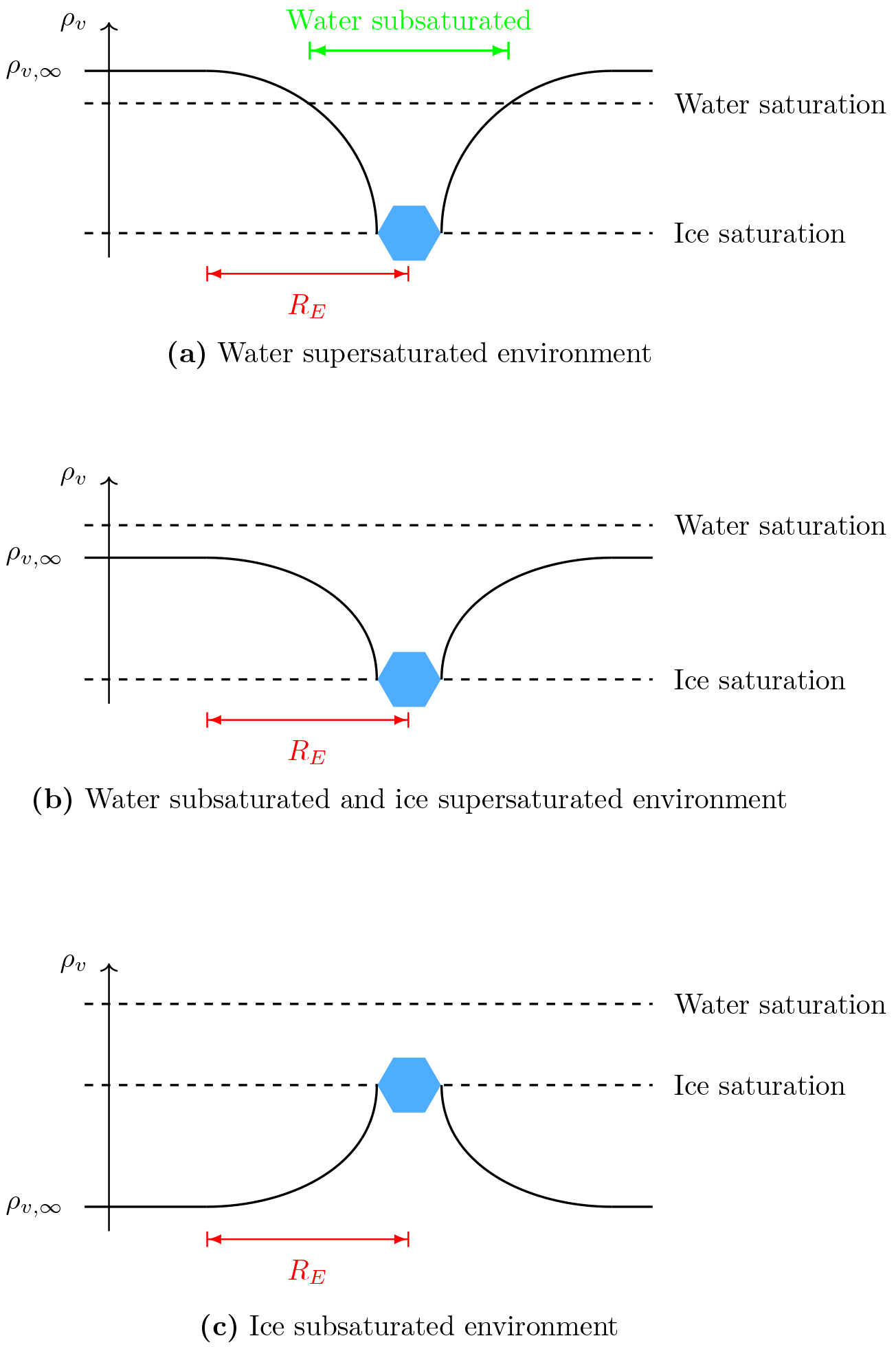
https://www.atmos-chem-phys.net/18/2525/2018/acp-18-2525-2018-f01

Figure 1Schematic of the water vapor density field around an ice crystal with various environmental water vapor values ρ_v,∞. Water vapor density at the ice crystal surface is assumed to equal the ice saturation density. In all cases, the ice crystal deforms the water vapor field locally within a ball of radius R_E. If a droplet has a distance smaller than R_E from the ice crystal, its growth behavior is determined by the local value of water density instead of the environmental value ρ_v,∞.

Download

In a mixed-phase cloud the picture may change dramatically since an ice crystal has a much more severe impact on the droplets in its vicinity: it may accelerate the evaporation of nearby droplets by growing at their expense. This local interaction is not new and is commonly referred to as the Wegener–Bergeron–Findeisen process (Bergeron, 1949; Findeisen, 1938; Wegener, 1911). Note that the Wegener–Bergeron–Findeisen process is different from the Ostwald ripening, in which bigger particles grow at the expense of smaller particles due to the curvature dependency of the saturation pressure (Lamb and Verlinde, 2011). Although the Wegener–Bergeron–Findeisen process is by definition a local process, numerical models do not represent it as such, since Maxwell's theory is applied and all hydrometeors grow according to the environmental rather than the local conditions. In Baumgartner and Spichtinger (2017), we investigated the impacts of local interactions by diffusion between an ice crystal and surrounding droplets qualitatively using a reference model that resolves the hydrometeors as well as the vapor and temperature fields. For convenience, we put the results from Baumgartner and Spichtinger (2017) into a “guiding schematic” illustrating the local water vapor field configurations; see Fig. 1. If a droplet has a distance smaller than R_E from the ice crystal, only the local value of water vapor density is seen by the droplet and therefore dictates its diffusional growth behavior. If the local droplet number is high enough, it influences the ice crystal and may even disconnect its growth behavior from the environmental conditions. In both cases, Maxwellian growth theory is not applicable. Apart from numerical simulations, the question of the solvability of the underlying governing equations is addressed in Baumgartner and Spichtinger (2018); for a reduced model problem existence and uniqueness of solutions could be proven.

In this study, we focus on a theoretical description of local interactions between an ice crystal and nearby droplets suited to be incorporated into a bulk-microphysical formulation. This study is organized as follows: Sect. 2 contains a derivation and a discussion of the model equations. In Sect. 3 we describe the incorporation of the new model into a simple parcel model in order to assess possible implications for a whole cloud. Finally we end with a summary and concluding remarks in Sect. 4.

2 Derivation of the model equations

This section is dedicated to the description and derivation of the model equations describing local interactions between an ice particle and surrounding cloud droplets. Section 2.1 contains the derivation. We comment on the choice of the involved parameters in Sect. 2.2 and afterwards present a model simplification in Sect. 2.3, while Sect. 2.4 contains a general discussion of the suggested model equations.

2.1 Local ice–droplet system

2.1.1 Description

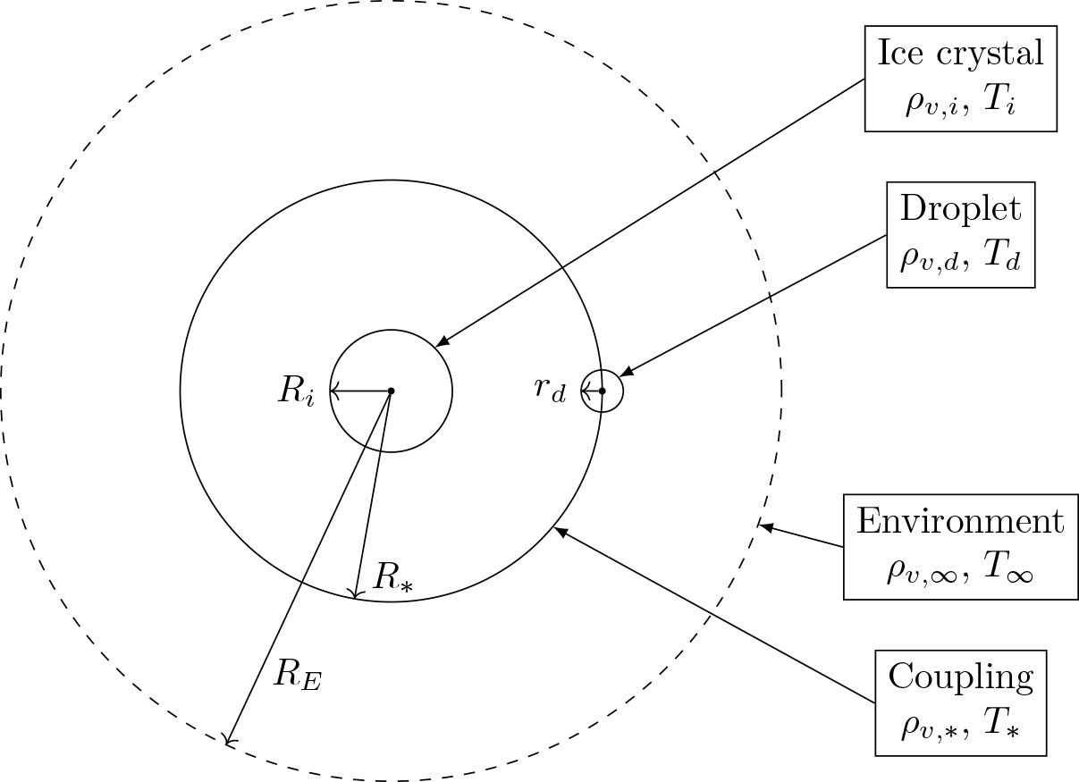
https://www.atmos-chem-phys.net/18/2525/2018/acp-18-2525-2018-f02

Figure 2Conceptual model of local ice–droplet system. In the center is an ice crystal with radius R_i and at distance R_∗ from the ice crystal is a cloud droplet with radius r_d. The presence of the ice crystal gives rise to an influence sphere with radius R_E around the ice crystal. Distance R_∗ is the coupling distance at which the diffusional growth of the hydrometeors is coupled.

Download

As a conceptual model for a local configuration of an ice crystal and a droplet, we consider the schematic shown in Fig. 2. A spherical ice crystal with radius R_i is located in the center. Water vapor density and temperature at the surface of the ice crystal are denoted by ρ_v,i and T_i, respectively. A droplet with radius r_d is located at distance R_∗ from the ice crystal center. We henceforth call R_∗ the “coupling distance” of the ice crystal–droplet interaction. Let ρ_v,d and T_d denote water vapor density and temperature at the surface of the droplet, respectively. Radius R_E denotes the “radius of influence” of the ice crystal, defined as the radius at which the ice crystal deforms the surrounding fields of water vapor and temperature in a non-negligible manner. We will discuss a possible choice of the radius of influence in Sect. 2.2.2, in which we regard the vapor field as deformed in a non-negligible manner if the relative deviation of the local value and the ambient value exceeds 0.1 %. The radius of influence gives rise to a “sphere of influence” around the ice crystal, wherein its influence on the fields for water vapor and temperature cannot be ignored. The values for water vapor density and temperature at the boundary of the influence sphere around the ice crystal are given by the environmental values ρ_v,∞ and T_∞. The corresponding values at coupling distance R_∗ are denoted by $ρ_{v, *}$ and T_∗. We will describe the local coupling of both hydrometeors with the help of the values $ρ_{v, *}$ and T_∗, so we call them the “coupling values”. Within this study, we denote variables referring to the properties of the ice crystal with uppercase letters and variables referring to the droplet with lowercase letters.

In this study, we always assume a spherical shape of the ice crystals and a negligible relative sedimentation velocity between the ice crystal and the neighboring droplet. Both assumptions are modeling assumptions. The assumption of a spherical ice crystal influences the growth behavior of the ice crystal and the growth behavior of the surrounding droplet; see Appendix A for an example. Including the effect of ice crystal shape on the diffusional growth of the surrounding droplet is beyond the scope of this study and would require precise information about the position of the droplet relative to the ice crystal, which is not available in models. In order to include the effect of the ice crystal shape on its own growth by diffusion, we could replace the growth Eq. (5a) with a variant using the ice crystal capacity (Lamb and Verlinde, 2011). Moreover, we could also replace the Maxwellian growth equation for the ice crystal with the model given in Chen and Lamb (1994) to model changes in ice crystal shape. Both modifications could improve the representation of the ice crystal growth, but also lead to an inconsistency in the model because in the following we need the assumption of spherical symmetry. Therefore we stick to the simpler growth equations.

As mentioned above, we consider water vapor and temperature fields as spherically symmetric inside the influence sphere as is done in Maxwellian growth theory. This assumption is not fully consistent with the schematic in Fig. 2, since spherical symmetry is not able to account for a spatial localized droplet as depicted in the schematic. Assuming spherical symmetric fields means that the droplet is replaced by a continuous source or sink for water vapor and temperature along the sphere with radius R_∗. This point of view also allows for generalization to the case of multiple droplets by appropriately changing the strength of the source or the sink.

As was done for the ice crystal, we may analogously define a sphere of influence for the droplet with corresponding radius of influence r_E. In order to use Maxwellian growth theory to describe droplet growth, we have to specify the values for water vapor density and temperature at the radius of influence r_E. We will use the coupling values $ρ_{v, *}$ and T_∗ as the environmental values in the droplet growth equation, i.e., as the values at the radius of influence r_E. With this choice, droplet growth responds to the coupling values.

The idea of the model is as follows. The ice crystal first establishes fields for water vapor and temperature as if it were isolated, yielding values at the coupling distance R_∗. These fields are given by the equilibrium fields for water vapor and temperature around the ice crystal and serve as background fields; see Eq. (1). Since the droplet is located at coupling distance R_∗, the coupling values $ρ_{v, *}$ and T_∗ define the ambient values for its diffusional growth. We establish an equation for the coupling values (see Eqs. 7 and 6), causing the droplet to grow or evaporate. This growth or evaporation feeds back to the coupling values and will in turn influence the growth behavior of the ice crystal.

In the following, we will derive the model equations resulting finally in the ODE system Eq. (19), consisting of the growth equations for the ice crystal (Eq. 19a and b), the growth equations of the droplet (Eq. 19c and d) and the evolution equations for the coupling values (Eq. 19e and f).

2.1.2 Derivation

The spherical symmetric solutions of the Laplace equations Δρ_v=0 and ΔT=0 for ρ_v and T inside the influence sphere of the ice crystal, describing the water vapor density and temperature field, are given by

\begin{array}{l} (1a) & ρ_{v} (R) = \frac{ρ_{v, \infty} R_{E} - ρ_{v, i} R_{i}}{R_{E} - R_{i}} + \frac{(ρ_{v, i} - ρ_{v, \infty}) R_{i} R_{E}}{R_{E} - R_{i}} \frac{1}{R}, \\ (1b) & T (R) = \frac{T_{\infty} R_{E} - T_{i} R_{i}}{R_{E} - R_{i}} + \frac{(T_{i} - T_{\infty}) R_{i} R_{E}}{R_{E} - R_{i}} \frac{1}{R}, \end{array}

where R is the radial distance from the ice crystal center. Equation (1) defines the unperturbed background fields for an isolated ice crystal, representing the spatial thermodynamic equilibrium. The corresponding solutions inside the influence sphere of the droplet are

\begin{array}{l} (2a) & \hat{ρ_{v}} (r) = \frac{ρ_{v, *} r_{E} - ρ_{v, d} r_{d}}{r_{E} - r_{d}} + \frac{(ρ_{v, d} - ρ_{v, *}) r_{E} r_{d}}{r_{E} - r_{d}} \frac{1}{r}, \\ (2b) & \hat{T} (r) = \frac{T_{*} r_{E} - T_{d} r_{d}}{r_{E} - r_{d}} + \frac{(T_{d} - T_{*}) r_{E} r_{d}}{r_{E} - r_{d}} \frac{1}{r}, \end{array}

where r is the radial distance from the droplet center. Proceeding as in the derivation of the Maxwellian growth equations, we obtain from Eq. (2) the following equations for the change in droplet mass and temperature

\begin{array}{l} (3a) & \frac{d m_{d}}{d t} = 4 π α_{d} D_{0} r_{d} r_{E} \frac{ρ_{v, *} - ρ_{v, d}}{r_{E} - r_{d}}, \\ \frac{d T_{d}}{d t} = \frac{4 π r_{d} r_{E}}{m_{d} c_{p, l} (T_{d}) (r_{E} - r_{d})} \\ (3b) & \cdot (L_{lv} (T_{d}) α_{d} D_{0} (ρ_{v, *} - ρ_{v, d}) + K_{0} (T_{*} - T_{d})), \end{array}

where m_d denotes the droplet mass, T_d the droplet temperature, α_d the accommodation coefficient (Davis, 2006), D₀ the diffusivity of air, K₀ the thermal conductivity of air, c_p,l the specific heat capacity of liquid water and L_lv the latent heat of vaporization. Using the representation of the water vapor field from Eq. (2), the rate J_d of water vapor exchange through the ball b_E with radius r_E around the droplet is given by

\begin{array}{l} J_{d} & = - \int_{\partial b_{E}} D_{0} \nabla \hat{ρ_{v}} \cdot N d σ = - D_{0} \frac{ρ_{v, *} - ρ_{v, d}}{r_{E} - r_{d}} \frac{r_{d}}{r_{E}} 4 π r_{E}^{2} \\ (4) & = - \frac{1}{α_{d}} \frac{d m_{d}}{d t}, \end{array}

where N denotes the outer normal vector at the surface ∂b_E.

The growth equations for the ice crystal are given by

\begin{array}{l} (5a) & \frac{d M_{i}}{d t} = 4 π α_{i} D_{0} R_{i} R_{*} \frac{ρ_{v, *} - ρ_{v, i}}{R_{*} - R_{i}}, \\ \frac{d T_{i}}{d t} = \frac{4 π R_{i} R_{*}}{M_{i} c_{p, i} (T_{i}) (R_{*} - R_{i})} \\ (5b) & \cdot (α_{i} D_{0} L_{i v} (T_{i}) (ρ_{v, *} - ρ_{v, i}) + K_{0} (T_{*} - T_{i})), \end{array}

where M_i denotes the ice crystal mass, T_i the ice crystal temperature, α_i the accommodation coefficient, c_p,i the specific heat of ice and L_iv the latent heat for sublimation. Note that in Eqs. (3) and (5) the coupling values $ρ_{v, *}$ and T_∗ show up to allow the coupling of the diffusional growth of the hydrometeors.

After the description of the respective growth equations, we proceed to the coupling values. We define

\begin{matrix} (6) & T_{*} (t) := T (R_{*}) and consequently \frac{d T_{*}}{d t} = \frac{d}{d t} (T (R_{*})), \end{matrix}

with T being the unperturbed background temperature field of the ice crystal from Eq. (1). As in Maxwellian growth theory, in definition Eq. (6) we assume temperature fluctuations to balance quickly and not to affect the droplet growth. We define the evolution equation for the coupling value $ρ_{v, *}$ as

\begin{matrix} (7) & \frac{d ρ_{v, *}}{d t} := I_{1} + I_{2} + I_{3}, \end{matrix}

being the sum of three terms I₁, I₂ and I₃ representing three different physical processes:

I₁ models the time evolution of the unperturbed water vapor field of the ice crystal,
I₂ takes the influence of the droplet on the coupling water vapor density into account and
I₃ describes the relaxation of the coupling value back to the value of the thermodynamic equilibrium ρ_v(R_∗).

The first term I₁ takes the unperturbed background value ρ_v(R_∗) of an isolated ice crystal into account. As the rate of change for this value, we define

\begin{matrix} (8) & I_{1} := \frac{d}{d t} (ρ_{v} (R_{*})) . \end{matrix}

If no droplet is present, we will have $I_{2} = I_{3} = 0$ in Eq. (7) and definition Eq. (8) simply ensures that $ρ_{v, *}$ equals the background value ρ_v(R_∗).

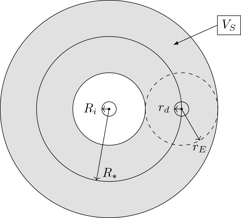
https://www.atmos-chem-phys.net/18/2525/2018/acp-18-2525-2018-f03

Figure 3Illustration of the spherical shell obtained by extending the surface of the sphere with interaction radius R_∗ around the ice crystal. Within the gray shaded area representing the volume V_S of the spherical shell, we assume a uniform distribution of water vapor and temperature.

Download

The second term I₂ considers the change in water vapor density due to droplet growth or evaporation. The rate of water vapor exchange J_d of the droplet is given in Eq. (4). The released water vapor is assumed to diffuse in unit time into some volume V to be defined later, leading to the water vapor exchange rate $\frac{J_{d}}{V}$ . Due to the assumed spherical symmetry, using the exchange rate $\frac{J_{d}}{V}$ directly amounts to assuming the sphere with radius R_∗ around the ice crystal as being filled up with droplets and their influence spheres, resulting in a strong overestimation of the droplet effect, so we have to rescale this rate. Assume the sphere with radius R_∗ around the ice crystal as being extended to a spherical shell with thickness 2r_E as in Fig. 3. This spherical shell is only introduced for the derivation of the coupling density Eq. (7). The value

\begin{array}{l} Z & := \frac{\frac{4}{3} π ((R_{*} + r_{E})^{3} - (R_{*} - r_{E})^{3})}{\frac{4}{3} π r_{E}^{3}} \\ (9) & = \frac{(R_{*} + r_{E})^{3} - (R_{*} - r_{E})^{3}}{r_{E}^{3}} \end{array}

measures the number of droplet influence spheres fitting inside the spherical shell. We take this value of Z to rescale the exchange rate and define the new value of I₂ as $\frac{J_{d}}{Z V}$ . In reality, influence spheres of droplets may also overlap, leading to another local competition for water vapor between the droplets and a larger value for Z. However, our choice assumes a local well-mixed droplet distribution around the ice crystal and we neglect a possible local competition between the droplets. If we consider not only a single droplet but in total N_d droplets inside the influence sphere of the ice crystal, we finally define the exchange rate as

\begin{matrix} (10) & I_{2} := N_{d} \frac{J_{d}}{Z V} = - \frac{N_{d}}{α_{d} Z V} \frac{d m_{d}}{d t}, \end{matrix}

where we used Eq. (4). This rate actually neglects local interactions and competitions between the droplets inside the influence sphere of the ice crystal and assumes all droplets as identical.

Finally, the third term I₃ accounts for the relaxation of the coupling value for water vapor density $ρ_{v, *}$ to ρ_v(R_∗), provided by the background field and representing thermodynamic equilibrium. Motivated by Fick's law of diffusion, let

\begin{matrix} (11) & - \int_{\partial B_{*}} D_{0} \frac{ρ_{v, *} - ρ_{v} (R_{*})}{R_{E} - R_{*}} d σ = - 4 π R_{*}^{2} D_{0} \frac{ρ_{v, *} - ρ_{v} (R_{*})}{R_{E} - R_{*}} \end{matrix}

be the rate of water vapor exchange from ball B_∗ to the outside, where B_∗ denotes the ball with coupling radius R_∗ around the ice crystal. The change in the coupling vapor density is therefore given by

\begin{array}{l} I_{3} & := - \int_{\partial B_{*}} D_{0} \frac{ρ_{v, *} - ρ_{v} (R_{*})}{R_{E} - R_{*}} d σ \frac{1}{\frac{4}{3} π R_{*}^{3}} \\ (12) & = - 3 D_{0} \frac{1}{R_{*}} \frac{ρ_{v, *} - ρ_{v} (R_{*})}{R_{E} - R_{*}} . \end{array}

Definition Eq. (12) represents a possible choice for the relaxation rate, but should ideally be reviewed with the help of measurements.

Altogether, substituting Eqs. (8), (10) and (12) into Eq. (7) yields

\begin{array}{l} (13) & \frac{d ρ_{v, *}}{d t} & = \frac{d}{d t} (ρ_{v} (R_{*})) + N_{d} \frac{J_{d}}{Z V} - \frac{3 D_{0}}{R_{*}} \frac{ρ_{v, *} - ρ_{v} (R_{*})}{R_{E} - R_{*}} \\ = \frac{d}{d t} (ρ_{v} (R_{*})) - \frac{N_{d}}{α_{d} Z V} \frac{d m_{d}}{d t} - \frac{3 D_{0}}{R_{*}} \frac{ρ_{v, *} - ρ_{v} (R_{*})}{R_{E} - R_{*}} \end{array}

for the rate of change of coupling water vapor density.

To define the volume V in Eq. (10), we first give an alternate interpretation of the rate $\frac{J_{d}}{Z V}$ with the help of the artificial spherical shell from Fig. 3. Let

\begin{matrix} (14) & V_{S} := \frac{4}{3} π ((R_{*} + r_{E})^{3} - (R_{*} - r_{E})^{3}) \end{matrix}

denote the volume of the artificial spherical shell. Using Eq. (9), the rate may be rewritten as

\begin{matrix} (15) & \frac{J_{d}}{Z V} = \frac{J_{d}}{V_{S}} \frac{\frac{4}{3} π r_{E}^{3}}{V} . \end{matrix}

The first factor represents the rate if all exchanged water vapor modified the vapor density inside the spherical shell, where we assume water vapor and temperature as uniform. The second factor amounts to a scaling of the first factor. Since V is the volume into which water vapor diffuses in unit time, we define it as a scaled influence sphere around the droplet as

\begin{matrix} (16) & V := \frac{4}{3} π (n r_{E})^{3} = \frac{4}{3} π n^{3} r_{E}^{3}, \end{matrix}

with the scaled influence radius nr_E leading to the rate $\frac{J_{d}}{Z V} = \frac{J_{d}}{V_{S}} \frac{1}{n^{3}}$ . With this definition, only a fraction $\frac{1}{n^{3}}$ of the released water vapor from the droplet will affect the coupling value inside the artificial spherical shell. The choice of the parameter n will be discussed in Sect. 2.2.4 below. Although we tried to give some interpretation of the product $\frac{J_{d}}{V_{S}} \frac{1}{n^{3}}$ and particularly the factor $\frac{1}{n^{3}}$ , this scaling factor may also be interpreted as a free parameter of our model without a specific physical meaning.

For the radii of influence R_E and r_E we define

\begin{array}{l} (17a) & R_{E} & := R_{i} + l_{i}, \\ (17b) & r_{E} & := r_{d} + l_{d}, \end{array}

for some positive constants l_i and l_d. Likewise, we define the coupling radius by

\begin{matrix} (18) & R_{*} := R_{i} + l_{0}, \end{matrix}

with $0 < l_{0} < l_{i}$ . With these definitions we can state the complete ODE system as

\begin{array}{l} (19a) & \frac{d m_{d}}{d t} = 4 π α_{d} D_{0} r_{d} r_{E} \frac{ρ_{v, *} - ρ_{v, d}}{r_{E} - r_{d}}, \\ \frac{d T_{d}}{d t} = \frac{4 π r_{d} r_{E}}{m_{d} c_{p, l} (T_{d}) (r_{E} - r_{d})} \\ (19b) & \cdot (α_{d} D_{0} L_{lv} (T_{d}) (ρ_{v, *} - ρ_{v, d}) + K_{0} (T_{*} - T_{d})), \\ (19c) & \frac{d M_{i}}{d t} = 4 π α_{i} D_{0} R_{i} R_{*} \frac{ρ_{v, *} - ρ_{v, i}}{R_{*} - R_{i}}, \\ \frac{d T_{i}}{d t} = \frac{4 π R_{i} R_{*}}{M_{i} c_{p, i} (T_{i}) (R_{*} - R_{i})} \\ (19d) & \cdot (α_{i} D_{0} L_{i v} (T_{i}) (ρ_{v, *} - ρ_{v, i}) + K_{0} (T_{*} - T_{i})), \\ (19e) & \frac{d ρ_{v, *}}{d t} = \frac{d}{d t} (ρ_{v} (R_{*})) + N_{d} \frac{J_{d}}{Z V} - \frac{3 D_{0}}{R_{*}} \frac{ρ_{v, *} - ρ_{v} (R_{*})}{R_{E} - R_{*}}, \\ (19f) & \frac{d T_{*}}{d t} = \frac{d}{d t} (T (R_{*})) . \end{array}

Substituting R_∗ from Eq. (18) into the field representations in Eq. (1) yields an expression of ρ_v(R_∗) and T(R_∗), allowing us to compute the required derivatives. Keeping Eqs. (17) and (18) in mind, we arrive at

\begin{array}{l} \frac{d}{d t} (ρ_{v} (R_{*})) & = \frac{R_{E}}{R_{E} - R_{i}} (1 - \frac{R_{i}}{R_{*}}) \frac{d ρ_{v, \infty}}{d t} \\ (20) & + \frac{R_{i}}{R_{E} - R_{i}} (\frac{R_{E}}{R_{*}} - 1) \frac{d ρ_{v, i}}{d t} \\ + \frac{ρ_{v, i} - ρ_{v, \infty}}{R_{E} - R_{i}} (\frac{R_{E} + R_{i}}{R_{*}} - \frac{R_{i} R_{E}}{R_{*}^{2}} - 1) \frac{d R_{i}}{d t} \end{array}

and

\begin{array}{l} \frac{d}{d t} (T (R_{*})) & = \frac{R_{E}}{R_{E} - R_{i}} (1 - \frac{R_{i}}{R_{*}}) \frac{d T_{\infty}}{d t} \\ (21) & + \frac{R_{i}}{R_{E} - R_{i}} (\frac{R_{E}}{R_{*}} - 1) \frac{d T_{i}}{d t} \\ + \frac{T_{i} - T_{\infty}}{R_{E} - R_{i}} (\frac{R_{E} + R_{i}}{R_{*}} - \frac{R_{i} R_{E}}{R_{*}^{2}} - 1) \frac{d R_{i}}{d t} . \end{array}

The derivative of the ice crystal radius may be calculated using the equation for the mass of a spherical ice crystal $M_{i} = \frac{4}{3} π ρ_{i} (T_{i}) R_{i}^{3}$ with ice density ρ_i, yielding

\begin{matrix} (22) & \frac{d R_{i}}{d t} = \frac{1}{4 π ρ_{i} (T_{i}) R_{i}^{2}} \frac{d M_{i}}{d t} = \frac{α_{i} D_{0}}{ρ_{i} (T_{i})} \frac{R_{*}}{R_{i}} \frac{ρ_{v, *} - ρ_{v, i}}{R_{*} - R_{i}}, \end{matrix}

where we neglected the derivative of the ice density ρ_i.

Neglecting the chemical composition and curvature effects of the ice crystal, we approximate the saturation vapor density ρ_v,i at the surface by

\begin{matrix} (23) & ρ_{v, i} \approx \frac{p_{i, sat} (T_{i})}{R_{v} T_{i}}, \end{matrix}

where p_i,sat denotes the saturation vapor pressure over a plane ice surface. Using the Clausius–Clapeyron equation (Lamb and Verlinde, 2011), we obtain the temporal derivative

\begin{array}{l} \frac{d ρ_{v, i}}{d t} & \approx \frac{d}{d t} (\frac{p_{i, sat} (T_{i})}{R_{v} T_{i}}) \frac{d T_{i}}{d t} \\ (24) & = \frac{p_{i, sat} (T_{i})}{R_{v} T_{i}^{2}} (\frac{L_{i v} (T_{i})}{R_{v} T_{i}} - 1) \frac{d T_{i}}{d t} . \end{array}

2.2 Choice of parameters

In this subsection we discuss a possible choice of the parameters $l_{i}, l_{d}, l_{0}, N_{d}$ and n from Eqs. (17), (18), (19e) and (16), respectively. We estimate possible values for these parameters using typical environmental conditions in a mixed-phase cloud with ambient temperature $T_{\infty} = - 15^{\circ} C$ , ambient pressure p_∞=650 hPa, ambient saturation ratio S_∞=1.01, ice crystal radius R_i=100 µm and droplet radius r_d=10 µm.

2.2.1 Parameter for droplet distance

Parameter l₀ in Eq. (18) defines the distance from the droplet center to the ice crystal surface. To estimate this parameter, we assume a perfectly regular distribution of droplets at the vertices of a cubic lattice with $N = 1000 {cm}^{- 3} = 10^{9} m^{- 3}$ droplets inside the cloud volume. This droplet number is higher than typical observed values, but since our focus is on local droplet accumulations around ice crystals, we use this higher value. Let

\begin{matrix} (25) & l_{K} := \frac{1}{\sqrt[3]{N} - 1 m^{- 1}} \end{matrix}

denote the edge length of a cuboid in the lattice. If the ice crystal is located in the center of such a cuboid, the distance from the midpoint of the ice crystal to the midpoint of the nearest droplet is given by $\frac{\sqrt{3}}{2} l_{K}$ , yielding an estimate for $R_{*} = R_{i} + l_{0}$ . By substituting values, we arrive at $l_{0} \approx 7.67 \times 10^{- 4} m = 767 µ m$ being approximately 7.5 times the ice radii, so l₀=7.5R_i.

2.2.2 Parameter for radii of the influence spheres

To estimate the distance parameter l_i determining the radius of the influence sphere of the ice crystal, we use the representation

\begin{matrix} (26) & ρ_{v} (R) = ρ_{v, \infty} - \frac{R_{i} (ρ_{v, \infty} - ρ_{v, i})}{R} \end{matrix}

of the water vapor field obtained from Maxwellian growth theory. Let ξ>0 denote a chosen maximal relative deviation of ρ_v(R) from the environmental value ρ_v,∞; we seek the radius R_E such that

\begin{matrix} (27) & \frac{|ρ_{v} (R) - ρ_{v, \infty}|}{ρ_{v, \infty}} \leq ξ \end{matrix}

is satisfied for R≥R_E. Substituting Eq. (26) into (27) yields the condition

\begin{matrix} (28) & \frac{R_{i}}{ξ ρ_{v, \infty}} |ρ_{v, \infty} - ρ_{v, i}| \leq R_{E} . \end{matrix}

Neglecting the effects of chemical substances and curvature, we estimate the surface water vapor density as $ρ_{v, i} = \frac{p_{i, sat} (T_{\infty})}{R_{v} T_{\infty}}$ .

Using a maximal relative deviation $ξ = 10^{- 3}$ , we arrive at l_i≈0.0144 m being approximately 144 ice radii, so l_i=144R_i. Using the same approach for the droplets, we obtain $l_{d} \approx 8.9 \times 10^{- 5} m$ being approximately 9 droplet radii, so l_d=9r_d. We chose $ξ = 10^{- 3}$ as the maximal relative deviation, because the relative deviations

\begin{matrix} (29) & \frac{|ρ_{v, \infty} - ρ_{v, i}|}{ρ_{v, \infty}} and \frac{|ρ_{v, \infty} - ρ_{v, d}|}{ρ_{v, \infty}} \end{matrix}

are already of the order of $1.4 \times 10^{- 1}$ and 10⁻², respectively, for the conditions stated at the beginning of the subsection. For the case of a droplet, Reiss and La Mer (1950) and Reiss (1951) suggest a value of 10 times the droplet diameter for the radius of influence. With our choice of the relative deviation, we obtain the same order of magnitude.

2.2.3 Number parameter

In order to estimate a typical droplet number N_d within the influence sphere around the ice crystal, we employ the typical droplet number concentration $N = 70 {cm}^{- 3}$ in mixed-phase clouds (Korolev et al., 2003; Zhao and Lei, 2014). Using l_i=144R_i, we obtain a droplet number

\begin{matrix} (30) & N_{d} = N \frac{4}{3} π (R_{i} + l_{i})^{3} = N \frac{4}{3} π (145 \cdot R_{i})^{3} \approx 894 . \end{matrix}

Not all of these droplets are precisely at coupling distance R_∗ from the midpoint of the ice crystal and the influence of droplets decreases with increasing distance from ice crystal center. Qualitatively, only the droplets closest to the ice crystal influence its growth behavior significantly; see Baumgartner and Spichtinger (2017). We employ the conservative assumption that all droplets with distances smaller than $\frac{R_{*}}{3}$ have larger influence on the ice crystal and consequently define the droplet number N_d as

\begin{matrix} (31) & N_{d} = N \frac{4}{3} π {(\frac{R_{i} + l_{0}}{3})}^{3} = N \frac{4}{3} π {(\frac{145}{3} R_{i})}^{3} \approx 32, \end{matrix}

motivating the choice N_d=40. We remark that this droplet number is highly variable in real clouds due to turbulent effects or sedimentation of the ice crystal. If one knew an expression describing the change in droplet number inside the influence sphere, one could also use a variable number instead of a constant.

2.2.4 Distribution parameter

Parameter n in Eq. (16) is a critical parameter of the whole model, since it directly determines the strength of the interaction between the ice crystal and the droplet. According to the interpretation given above, it describes which fraction of released water vapor from an evaporating droplet is incorporated into the artificial spherical shell around the ice crystal and consequently influences the growth of the ice crystal; see Eq. (15). If n=1, all released water vapor is incorporated in the artificial spherical shell. If n>1, only a fraction of $\frac{1}{n^{3}}$ is incorporated, and the remaining water vapor is released to the atmosphere. In this study, we use a value n=1.8 obtained with the help of direct numerical simulations using the reference model described in Baumgartner and Spichtinger (2017), since the authors are not aware of any direct measurements.

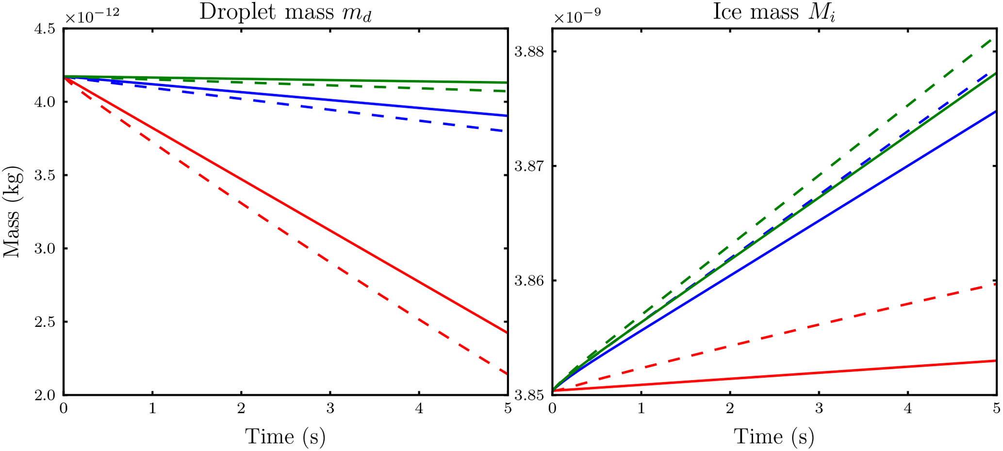
https://www.atmos-chem-phys.net/18/2525/2018/acp-18-2525-2018-f04

Figure 4Comparison of the temporal evolution of hydrometeor masses obtained with the new model from Eq. (19) with parameter value n=1.8 (dashed) and the reference model (solid) for the case of N_d=14 droplets per influence sphere. Ambient saturation ratios are S_∞=0.86 (red), S_∞=0.99 (blue) and S_∞=1.01 (green).

Download

https://www.atmos-chem-phys.net/18/2525/2018/acp-18-2525-2018-f05

Figure 5As in Fig. 4, but for the case of N_d=38 droplets per influence sphere.

Download

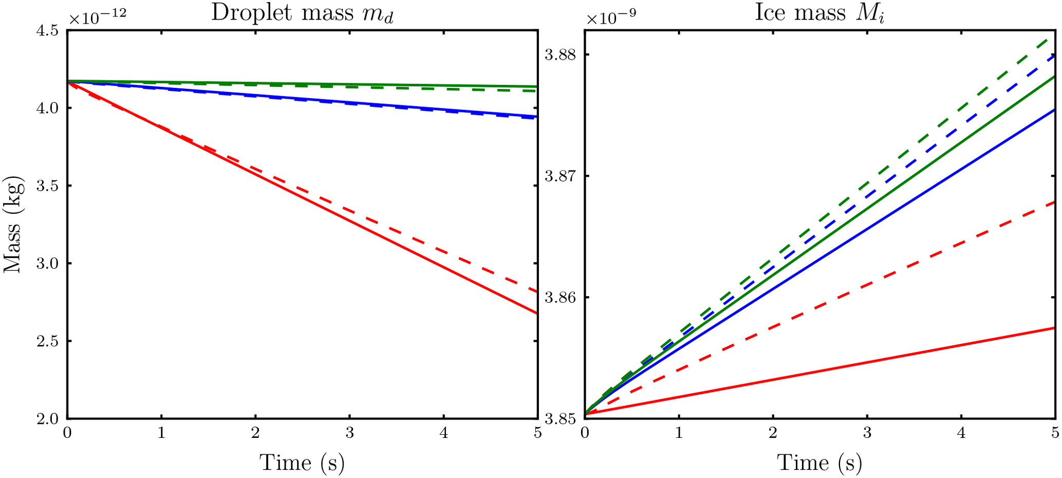
We compare the temporal evolution of the ice crystal and droplet mass obtained from the reference model with results from the model presented in Sect. 2.1 using the two droplet numbers N_d=14 and N_d=38. The choice of these droplet numbers is due to the existence of Lebedev quadrature formulas because those quadrature points allow a nearly uniform distribution along a sphere (Lebedev, 1976). For calculations with the reference model, we distributed the droplets along a sphere with radius 7.5R_i around the ice crystal. We conducted several simulations using the new model with different values for the parameter n. Figures 4 and 5 show the accordance of droplet and ice crystal mass evolution for our final parameter value n=1.8 at ambient saturation ratios S_∞=0.86, S_∞=0.99 and S_∞=1.01 for the two droplet numbers N_d=14 and N_d=38. The solid and dashed curves agree well, although the droplet masses are slightly underestimated and the ice crystal mass is slightly overestimated.

Although not shown, numerical experiments with other values of the parameter n show that we can achieve better agreement of either the ice mass or droplet curves, but not for both simultaneously. Moreover, our choice n=1.8 also shows satisfactory results in other mass and humidity regimes.

2.3 Simplifications

The model in Eq. (19) consists of many equations, and it especially keeps track of the temperature of the individual hydrometeors. In Maxwellian growth theory, the equation for the temperature of a hydrometeor is eliminated. We can simplify the model in Eq. (19) in a similar way. Proceeding as in the derivation of the Maxwellian growth equations, we can eliminate the temperature equations of the hydrometeors. The modified equations for the hydrometeor masses are then given by

\begin{array}{l} \frac{d m_{d}}{d t} = \frac{4 π}{(\frac{L_{lv} (T_{\infty})}{R_{v} T_{\infty}} - 1) \frac{L_{lv} (T_{\infty})}{K_{0} T_{\infty}} + \frac{R_{v} T_{\infty}}{α_{d} D_{0} p_{l, sat} (T_{\infty})}} \frac{r_{d} r_{E}}{r_{E} - r_{d}} (S_{*} - 1) \\ (32) & = : G_{l} \frac{r_{d} r_{E}}{r_{E} - r_{d}} (S_{*} - 1) \end{array}

for droplet mass and

\begin{array}{l} \frac{d M_{i}}{d t} = \frac{4 π}{(\frac{L_{i v} (T_{\infty})}{R_{v} T_{\infty}} - 1) \frac{L_{i v} (T_{\infty})}{K_{0} T_{\infty}} + \frac{R_{v} T_{\infty}}{α_{i} D_{0} p_{i, sat} (T_{\infty})}} \frac{R_{i} R_{*}}{R_{*} - R_{i}} (S_{*, i} - 1) \\ (33) & = : G_{i} \frac{R_{i} R_{*}}{R_{*} - R_{i}} (S_{*, i} - 1) \end{array}

for ice crystal mass with the saturation ratios $S_{*} = \frac{ρ_{v, *} R_{v} T_{\infty}}{p_{l, sat} (T_{\infty})}$ and $S_{*, i} = \frac{ρ_{v, *} R_{v} T_{\infty}}{p_{i, sat} (T_{\infty})}$ , respectively, where p_l,sat denotes the saturation vapor pressure over a plane surface of liquid water. In addition, we neglect the temperature Eq. (19f) for the coupling temperature T_∗ in the governing system Eq. (19). Since T_∗ also appears in the calculation of the unperturbed value ρ_v(R_∗) through the equilibrium vapor density at the ice crystal surface, we have to modify its calculation from Eq. (1). We simplify the vapor density field from Eq. (1) by considering the case R_E→∞ representing the observation R_i≪R_E. The vapor density at the ice crystal surface is approximated as in Eq. (23), yielding

\begin{array}{l} ρ_{v} (R_{*}) & \approx ρ_{v, \infty} + (ρ_{v, i} - ρ_{v, \infty}) \frac{R_{i}}{R_{*}} \\ (34) & \approx ρ_{v, \infty} + (\frac{p_{i, sat} (T_{\infty})}{R_{v} T_{\infty}} - ρ_{v, \infty}) \frac{R_{i}}{R_{*}} . \end{array}

Using the Clausius–Clapeyron equation and Eq. (22), we compute the required time derivative of Eq. (34) as

\begin{array}{l} \frac{d}{d t} (ρ_{v} (R_{*})) & \approx (1 - \frac{R_{i}}{R_{*}}) \frac{d ρ_{v, \infty}}{d t} + \frac{R_{i}}{R_{*}} \frac{d}{d t} (\frac{p_{i, sat} (T_{\infty})}{R_{v} T_{\infty}}) \\ + (\frac{p_{i, sat} (T_{\infty})}{R_{v} T_{\infty}} - ρ_{v, \infty}) \frac{R_{*} - R_{i}}{R_{*}^{2}} \frac{d R_{i}}{d t} \\ (35) & = (1 - \frac{R_{i}}{R_{*}}) \frac{d ρ_{v, \infty}}{d t} \\ + \frac{R_{i}}{R_{*}} \frac{p_{i, sat} (T_{\infty})}{R_{v} T_{\infty}^{2}} (\frac{L_{i v} (T_{\infty})}{R_{v} T_{\infty}} - 1) \frac{d T_{\infty}}{d t} \\ + (\frac{p_{i, sat} (T_{\infty})}{R_{v} T_{\infty}} - ρ_{v, \infty}) \frac{R_{*} - R_{i}}{4 π ρ_{i} (T_{\infty}) R_{i}^{2} R_{*}^{2}} \frac{d M_{i}}{d t} . \end{array}

Accepting those further approximations, we arrive at the simplified system

\begin{array}{l} (36a) & \frac{d m_{d}}{d t} = G_{l} \frac{r_{d} r_{E}}{r_{E} - r_{d}} (S_{*} - 1), \\ (36b) & \frac{d M_{i}}{d t} = G_{i} \frac{R_{i} R_{*}}{R_{*} - R_{i}} (S_{*, i} - 1), \\ \frac{d ρ_{v, *}}{d t} = \frac{d}{d t} (ρ_{v} (R_{*})) - \frac{N_{d}}{α_{d} Z V} \frac{d m_{d}}{d t} \\ (36c) & - \frac{3 D_{0}}{R_{*}} \frac{ρ_{v, *} - ρ_{v} (R_{*})}{R_{E} - R_{*}}, \end{array}

where only the three prognostic variables m_d, M_i and $ρ_{v, *}$ are left. For a bulk model parameterization, we would add just one additional equation.

2.4 Discussion of the model ansatz

Srivastava (1989) has already criticized the use of Maxwellian growth theory for the description of droplet growth by diffusion. He advocated the use of local quantities instead of the environmental conditions, since water vapor density is spatially variable and the droplet growth heavily depends on its precise value. By using local variables, one can take those variations into account and compute growth rates of hydrometeors more accurately. He connected the local value for vapor density to the environmental value through a relaxation of local conditions to the environmental conditions, similarly as we did in Eq. (12) for I₃. Srivastava proposed considering local volumes around every hydrometeor and computing its individual growth rate by using the local vapor density. We adopted this approach in our model by introducing the “spheres of influence”. Similar ideas were employed in Marshall and Langleben (1954), in which the authors also consider a local volume around an ice crystal. In contrast to our formulation, they assume a continuous droplet distribution inside the local volume. Their method avoids additional growth equations for the nearby droplets. Our approach combines ideas from both former studies, whereby we focused on a model formulation that only incorporates values that are typically known in a numerical cloud model.

In Sect. 2.2, we estimated possible values for the parameters of our model. To our best knowledge, there are no direct measurements of the local interactions of a single ice crystal with surrounding droplets available, so we cannot compare our parameter choice with real measurements. Instead we can consider two separate extreme cases, since Eq. (19e) for the coupling water vapor density has the generic representation

\begin{matrix} (37) & \frac{d ρ_{v, *}}{d t} = \frac{d}{d t} (ρ_{v} (R_{*})) - \frac{N_{d}}{Z V} \frac{d m_{d}}{d t} - C (ρ_{v, *} - ρ_{v} (R_{*})) \end{matrix}

for a constant C>0. In our model derivation, we set $C := \frac{3 D_{0}}{R_{*} (R_{E} - R_{*})}$ . The two extreme cases are constructed by choosing C=0 or C→∞. In the first case C=0, relaxation of the coupling value $ρ_{v, *}$ to the equilibrium value ρ_v(R_∗) is neglected and therefore $ρ_{v, *}$ is solely changed by the growth or evaporation of the hydrometeors. The second case C→∞ corresponds to an instantaneous relaxation to equilibrium. This is basically the same behavior as in the classical treatment using Maxwellian growth theory. We emphasize that both extreme cases are rather nonphysical, but they may serve to assess the possible strength of the local interactions. However, we believe that the ansatz from Eq. (37) is able to capture the essential behavior, possibly after considering $\frac{1}{Z V}$ as a single coefficient that is to be determined with the help of measurements.

We believe that the most promising measurement technology to constrain the parameters in our model is holography because it is able to measure the spatial distribution and the size of hydrometeors within an air volume (Beals et al., 2015; Fugal and Shaw, 2009; Schlenczek et al., 2017). Moreover, if it were possible to track an individual air volume with holographic imaging, one could possibly infer values for our model constants from the size evolutions of the hydrometeors.

In Sect. 2.2.3 we discussed the choice of the number N_d of droplets within the influence sphere of the ice crystals. Imaging the influence sphere around the ice crystal as an object moving with the ice crystal, clearly the number of droplets inside this region should change as the ice crystal moves through a cloudy volume. If we could establish an equation for $\frac{d N_{d}}{d t}$ , the number N_d of droplets within the influence sphere could be made dynamic. Such an equation should account not only for the movement of the ice crystal through the cloudy volume but also for the influence of turbulence on the local droplet number. Note that the concept of an influence sphere around the ice crystal remains meaningful for moving ice crystals. The presence of the ice crystal distorts the local water vapor and temperature field and thus defines its influence sphere. As is well known from Maxwellian growth theory, the fields around the ice crystal very rapidly attain their steady state (Lamb and Verlinde, 2011), so we can define the influence sphere with the help of the steady-state field.

3 Incorporation into a parcel model

In this section, we incorporate the new model from Sect. 2 into a parcel model. Let p_∞ and T_∞ denote the pressure and temperature of the air parcel. We divide the total water mass contained in the air parcel into the mass of water vapor M_v, the mass of liquid water M_l and the mass of ice M_ice. In addition, the air parcel contains a mass M_a of dry air. Since the air parcel is assumed as thermodynamically closed, the mass M_a of dry air and the total water mass $M_{v} + M_{l} + M_{ice}$ are constant. Instead of the masses, we consider the mixing ratios $q_{x} := \frac{M_{x}}{M_{a}}$ for $x \in {v, l, ice}$ .

3.1 Description of the parcel model

Variations in pressure p_∞ are governed by the equation

\begin{matrix} (38) & \frac{d p_{\infty}}{d t} = \frac{d p_{\infty}}{d z} \frac{d z}{d t} = - g \frac{p_{\infty}}{\overline{R} T_{\infty}} w, \end{matrix}

which is obtained by applying the equation for hydrostatic equilibrium. Coordinate z denotes the height, g the acceleration of gravity, w the vertical velocity and $\overline{R}$ the gas constant for moist air given by

\begin{matrix} (39) & \overline{R} := R_{a} (1 + \frac{1 - ε}{ε} \frac{q_{v}}{1 + q_{v}}), \end{matrix}

where $ε := \frac{R_{a}}{R_{v}}$ and R_a,R_v denote the gas constants for dry air and water vapor, respectively. A change in the air parcel temperature T_∞ has two contributions. The first contribution comes from the adiabatic vertical motion of the air parcel and is given by (Wang, 2013)

\begin{matrix} (40) & {\frac{d T_{\infty}}{d t}|}_{adiabatic} = - \frac{g}{\overline{c_{p}}} w, \end{matrix}

where the specific heat capacity of moist air is given by (Rogers and Yau, 1989)

\begin{matrix} (41) & \overline{c_{p}} := c_{p, a} (1 + (\frac{c_{p, v}}{c_{p, a}} - 1) \frac{q_{v}}{1 + q_{v}}), \end{matrix}

and c_p,a and c_p,v denote the specific heat capacity of dry and moist air, respectively. If the condensation of water vapor takes place, we have to include latent heat effects. Let ω_k be a hydrometeor; its temperature T_k changes as

\begin{matrix} (42) & c_{p, k} m_{k} \frac{d T_{k}}{d t} = L \frac{d m_{k}}{d t} + \int_{\partial ω_{k}} K \nabla T \cdot N d σ, \end{matrix}

where m_k is the mass of hydrometeor ω_k, L the latent heat of a phase change, K the thermal conductivity of air and N the outer normal to the surface of the hydrometeor ω_k. The surface integral in Eq. (42) accounts for heat conduction from the hydrometeor to the air parcel. The amount of heat −dQ_conduction delivered from the single hydrometeor ω_k to the air parcel is given by the rate

\begin{matrix} (43) & - \frac{d Q_{conduction}}{d t} = \int_{\partial ω_{k}} K \nabla T \cdot N d σ . \end{matrix}

This amount of heat changes the temperature T_∞ of the air parcel according to $\overline{c_{p}} (M_{v} + M_{a}) d T_{\infty} = - d Q_{conduction}$ . Inserting Eq. (43) and summing over all hydrometeors yields the rate

\begin{matrix} (44) & {\frac{d T_{\infty}}{d t}|}_{latent} = - \frac{1}{\overline{c_{p}} (M_{v} + M_{a})} \sum_{k} \int_{\partial ω_{k}} K \nabla T \cdot N d σ \end{matrix}

of latent heating. Combining both contributions from Eqs. (40) and (44) yields the final rate of the temperature change

\begin{array}{l} \frac{d T_{\infty}}{d t} & = {\frac{d T_{\infty}}{d t}|}_{adiabatic} + {\frac{d T_{\infty}}{d t}|}_{latent} \\ (45) & = - \frac{g}{\overline{c_{p}}} w - \frac{1}{\overline{c_{p}} (M_{v} + M_{a})} \sum_{k} \int_{\partial ω_{k}} K \nabla T \cdot N d σ, \end{array}

where the sum expands over all hydrometeors. In the literature, one finds a slightly different equation in which the surface integral is replaced by $- L \frac{d m_{k}}{d t}$ (Pruppacher and Klett, 1997). Assuming all hydrometeors to have reached their equilibrium temperature, as is done in classical Maxwellian growth theory, the time derivative on the left-hand side of Eq. (42) vanishes and Eq. (45) reduces to the equation from the literature.

We further divide the liquid water mass M_l contained in the air parcel into the mass $M_{l}^{i}$ of all droplets located in an influence sphere of some ice crystal and the mass $M_{l}^{o}$ of all droplets outside of every ice crystal influence sphere. From now on, we assume a monodisperse mass distribution for the ice crystals with number concentration 𝒩_ice for the droplets inside the ice crystal influence spheres with number concentration 𝒩_iceN_d (number of ice influence spheres containing N_d droplets each) and and for the droplets outside of every ice crystal influence sphere with number concentration $N_{d}^{o}$ . Therefore, the total droplet number concentration in the air parcel is $N_{ice} N_{d} + N_{d}^{o}$ (number per kilogram of dry air). Because of the assumption of monodisperse size distributions, each ice particle has mass M_i, each droplet inside an influence sphere has mass $m_{d}^{i}$ and each droplet outside of every influence sphere has mass $m_{d}^{o}$ . Defining the liquid water mixing ratios $q_{l}^{i} := \frac{M_{l}^{i}}{M_{a}}$ and $q_{l}^{o} := \frac{M_{l}^{o}}{M_{a}}$ , we obtain the relations

\begin{matrix} (46) & q_{ice} = N_{ice} M_{i} and q_{l} = q_{l}^{o} + q_{l}^{i} = N_{d}^{o} m_{d}^{o} + N_{d} N_{ice} m_{d}^{i} \end{matrix}

where N_d is the number of droplets inside the influence sphere of an ice crystal. As for the liquid water mass, we divide the corresponding droplet temperatures in $T_{d}^{i}$ and $T_{d}^{o}$ and the droplet radii in $r_{d}^{i}$ and $r_{d}^{o}$ .

Using this notation and the assumption of spherical droplets, we can evaluate the surface integrals in Eq. (45) to obtain

\begin{array}{l} \frac{d T_{\infty}}{d t} = - \frac{g}{\overline{c_{p}}} w - \frac{1}{\overline{c_{p}} (M_{v} + M_{a})} (N_{d}^{o} M_{a} 4 π r_{d}^{o} K_{0} (T_{\infty} - T_{d}^{o}) \\ + N_{d} N_{ice} M_{a} 4 π r_{d}^{i} K_{0} (T_{\infty} - T_{d}^{i}) + N_{ice} M_{a} 4 π R_{i} K_{0} (T_{\infty} - T_{i})) \\ = - \frac{g}{\overline{c_{p}}} w - \frac{4 π K_{0} M_{a}}{\overline{c_{p}} (M_{v} + M_{a})} (N_{d}^{o} r_{d}^{o} (T_{\infty} - T_{d}^{o}) \\ + N_{d} N_{ice} r_{d}^{i} (T_{\infty} - T_{d}^{i}) + N_{ice} R_{i} (T_{\infty} - T_{i})) \\ = - \frac{g}{\overline{c_{p}}} w - \frac{4 π K_{0}}{\overline{c_{p}} (1 + q_{v})} (N_{d}^{o} r_{d}^{o} (T_{\infty} - T_{d}^{o}) \\ (47) & + N_{d} N_{ice} r_{d}^{i} (T_{\infty} - T_{d}^{i}) + N_{ice} R_{i} (T_{\infty} - T_{i})), \end{array}

where R_i denotes the radius of an ice crystal. The mixing ratio for water vapor is determined by the conservation of mass and reads

\begin{array}{l} \frac{d q_{v}}{d t} = - \frac{d q_{l}^{o}}{d t} - \frac{d q_{l}^{i}}{d t} - \frac{d q_{ice}}{d t} \\ (48) & = - N_{d}^{o} \frac{d m_{d}^{o}}{d t} - N_{ice} (N_{d} \frac{d m_{d}^{i}}{d t} + \frac{d M_{i}}{d t}) . \end{array}

The equations for the other mixing ratios are given by

\begin{array}{l} (49a) & \frac{d q_{ice}}{d t} = N_{ice} \frac{d M_{i}}{d t}, \\ (49b) & \frac{d q_{l}^{o}}{d t} = N_{d}^{o} \frac{d m_{d}^{o}}{d t}, \\ (49c) & \frac{d q_{l}^{i}}{d t} = N_{d} N_{ice} \frac{d m_{d}^{i}}{d t} . \end{array}

3.2 Results

Using the parcel model we carry out several simulations in which we vary the coupling distance $R_{*} = R_{i} + l_{0}$ through parameter l₀, the number of droplets inside the influence sphere of the ice crystals N_d, the ambient saturation ratio S_∞ and the vertical velocity w of the air parcel; see Table 1. The choice of the saturation ratios is motivated by the three regimes in Fig. 1.

Table 1Different parameter values used for the air parcel simulations. The initial ice crystal radius is R_i=100 µm for every simulation.

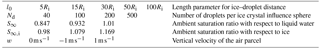
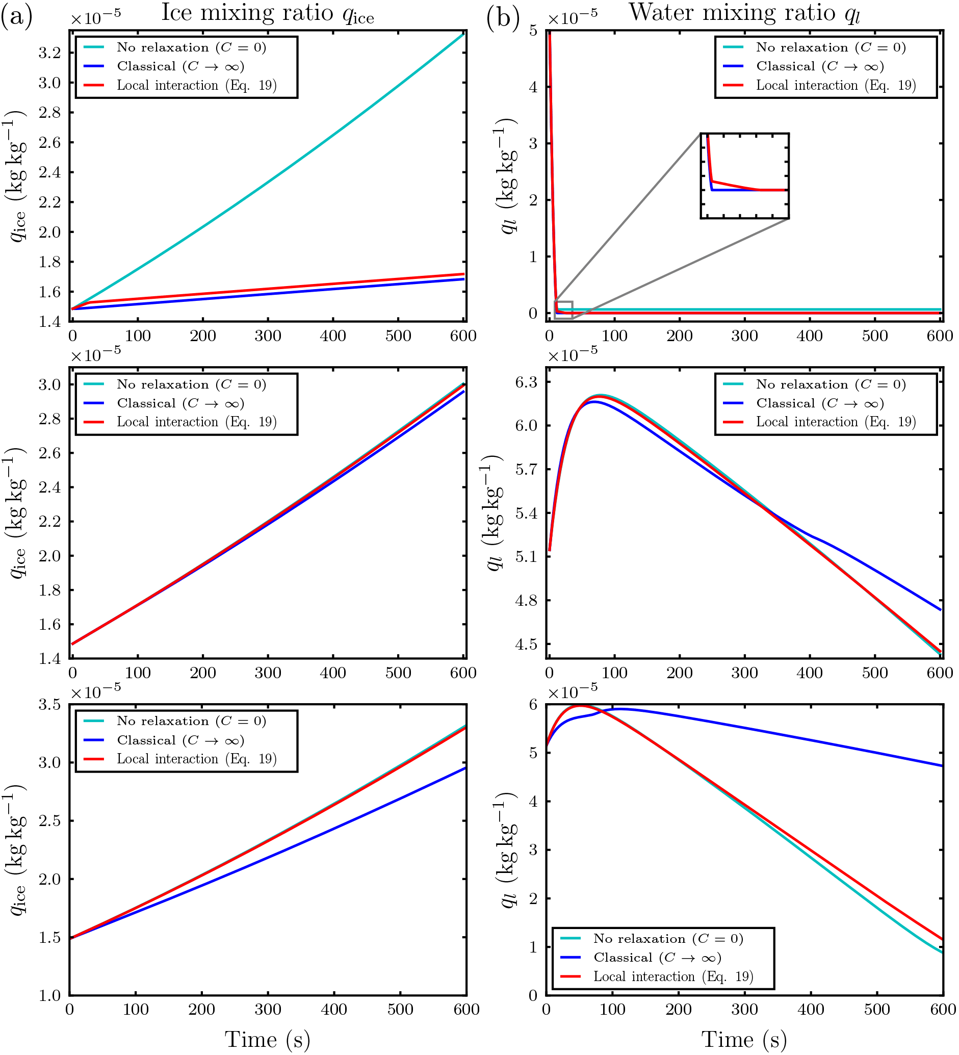
Download Print Version | Download XLSX

https://www.atmos-chem-phys.net/18/2525/2018/acp-18-2525-2018-f06

Figure 6Temporal evolution of ice mixing ratio (a) and liquid water mixing ratio (b) for the parcel model simulations with $w = 0 m s^{- 1}$ . Parameters for the first row are N_d=40 droplets in each influence sphere of the ice crystals at initial ambient saturation ratio S_∞=0.847 and droplet distance l₀=5R_i. The second and third row both have N_d=500 droplets per influence sphere at S_∞=1.01, while the droplet distance is l₀=30R_i for the second row and l₀=5R_i for the third row. Note the different scaling of the axes.

Download

The initial values for ambient temperature and pressure are $T_{\infty} = - 15^{^{\circ}} C$ and p_∞=650 hPa, respectively, resembling typical environmental conditions for a mixed-phase cloud. Reliable values for the droplet number N_d inside every influence sphere of the ice crystals are difficult to estimate, since this depends heavily on small-scale turbulence. Therefore, any of the estimated values in Sect. 2.2.3 between N_d=30 and N_d=800 is possible, explaining the choices in Table 1.

Previous studies indicate a large scattering of the microphysical parameters, especially in liquid water content (LWC) and ice water content (IWC) (Fleishauer et al., 2002; Hobbs et al., 2001; Lloyd et al., 2015; Noh et al., 2013; Pinto et al., 2001; Verlinde et al., 2007; Zhao and Lei, 2014). We use the typical values $LWC = 0.045 {gm}^{- 3}$ (Korolev et al., 2003) and $IWC = 0.013 {gm}^{- 3}$ (Fleishauer et al., 2002). A typical droplet radius is given as 10 µm. Variability in the size of the ice crystals is much larger, but on average pristine ice crystals in mixed-phase clouds tend to be smaller than in ice clouds (Korolev et al., 2003) and we again use a value of 100 µm as the initial radius.

In the subsequent sections, we present simulation results ordered by vertical velocity. All figures contain three curves: the red curve represents the solution of the new system Eq. (19), the cyan and blue curves represent the solutions of the same system, in which the equation for the coupling water vapor density Eq. (19e) is replaced by Eq. (37) with C=0 and C→∞, respectively. Consequently, those two curves correspond to the extreme cases without local relaxation to equilibrium (case C=0) and instantaneous relaxation to equilibrium (case C→∞). The spreading between the two curves shows the spectrum of possible values for different choices of the parameter C.

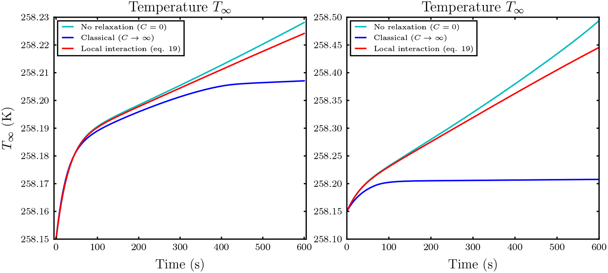
https://www.atmos-chem-phys.net/18/2525/2018/acp-18-2525-2018-f07

Figure 7Temporal evolution of the air parcel temperature T_∞ with $w = 0 m s^{- 1}$ and N_d=500 per influence sphere of the ice crystals at initial ambient saturation ratio S_∞=1.01 with droplet distance l₀=30R_i (a) and l₀=5R_i (b). Note the different scaling of the axes.

Download

3.2.1 Vertical velocity $w = 0 m s^{- 1}$

In Baumgartner and Spichtinger (2017), the authors documented the largest effect of surrounding droplets on ice growth in an ice subsaturated environment because the evaporating droplets can deliver enough water vapor towards the ice crystal to produce a local supersaturation with respect to ice, allowing the crystal to grow instead of evaporate. With the new model, we also observe a similar behavior. Consider, for example, the case of N_d=40 droplets per influence sphere of any ice crystal with the small droplet distance $l_{0} = 5 R_{i} = 5 \times 100 µ m$ from the ice crystal and ambient saturation ratio S_∞=0.847, being subsaturated with respect to ice and water. The first row in Fig. 6 shows the temporal evolution of the ice mixing ratio q_i and liquid water mixing ratio q_l. We observe an increasing ice mixing ratio q_i, showing the aforementioned local interaction. As long as not all droplets inside the influence spheres are evaporated, the red curve for the ice mixing ratio in Fig. 6 coincides with the cyan curve, indicating the extreme case without local relaxation. This means that the evaporating droplets inside the influence sphere of the ice crystal provide enough water vapor to mostly compensate diffusion of water vapor to the environment. The red curve in the upper panel in Fig. 6b shows the temporal evolution of the liquid water mixing ratio q_l. At the first kink of this curve (at about t=11 s), all droplets outside of the influence spheres are evaporated ( $q_{l}^{o} = 0$ ) and at the second kink (at about t=26 s) the droplets inside the influence spheres are also evaporated, indicating $q_{l} = q_{l}^{o} = q_{l}^{i} = 0$ . Although the environment is subsaturated with respect to ice, the evaporating ice crystals alleviate the local subsaturation, allowing the droplets inside the influence spheres to exist slightly longer; see case (c) in the schematic Fig. 1. The kink in the red curve for the ice mixing ratio in in the upper panel in Fig. 6a at about t=26 s marks the time instant at which all droplets are evaporated. From this time on, the local source for water vapor vanishes and the ice crystals grow slower. Note that the evaporated droplets provided enough water vapor to the whole air parcel to cause an ice supersaturated environment (see Fig. B1 in the Appendix), explaining why the ice crystals continue to grow although the air parcel was initially subsaturated with respect to ice.

By changing the environmental conditions to water supersaturation with S_∞=1.01, local effects on the mixing ratios are almost not visible. Only for small distances such as l₀=5R_i of the droplets in the influence spheres from the ice crystals or very high droplet numbers N_d is an effect on the mixing ratios observed; for the case of a droplet–ice distance of l₀=30R_i and droplet number N_d=500, see the middle row in Fig. 6. The more interesting variable in this humidity regime is the temperature T_∞ of the air parcel shown in the left panel of Fig. 7 for the aforementioned case. Compared to the classical treatment, including the local effects yields a slightly warmer air parcel. The heating is caused by the release of latent heat from the growing hydrometeors. It persists after 100 s at which the droplet mass starts to decrease and the evaporating droplets tend to cool the air parcel (right panel in the middle row of Fig. 6). Therefore, the observed heating is due to the growth of the ice crystals and should increase for increasing ice growth rate.

This motivates us to consider the case of a small droplet–ice distance l₀=5R_i and high droplet number N_d=500 at ambient saturation ratio S_∞=1.01. The effect on the air parcel temperature T_∞ for this case is shown in the right panel of Fig. 7. The lower row in Fig. 6 shows an increase in ice mixing ratio and a decrease in liquid water mixing ratio already after a short time. This again confirms that the observed heating of the air parcel is caused by an increased growth rate of the ice crystals. The increase of the ice crystal growth rate is influenced by the number N_d of droplets within the influence sphere and the ambient saturation ratio. If the air parcel is initially supersaturated with respect to water, the ice crystal induces a local subsaturation with respect to water and the droplets inside the influence sphere start to evaporate; see case (a) in the schematic in Fig. 1. The evaporation of nearby droplets enhances the local water vapor density and consequently also the ice growth rate. If the air parcel is initially subsaturated with respect to water, the droplets inside the influence sphere of an ice crystal see two sinks of water vapor, namely the ice crystal and the environment; see case (b) in the schematic Fig. 1. The released water vapor of an evaporating droplet is therefore partially delivered to the ice crystal and the environment, and the growth rate of the ice crystal is less amplified. Consequently, we expect a larger effect of the local interactions on the air parcel temperature with initially water supersaturated conditions.

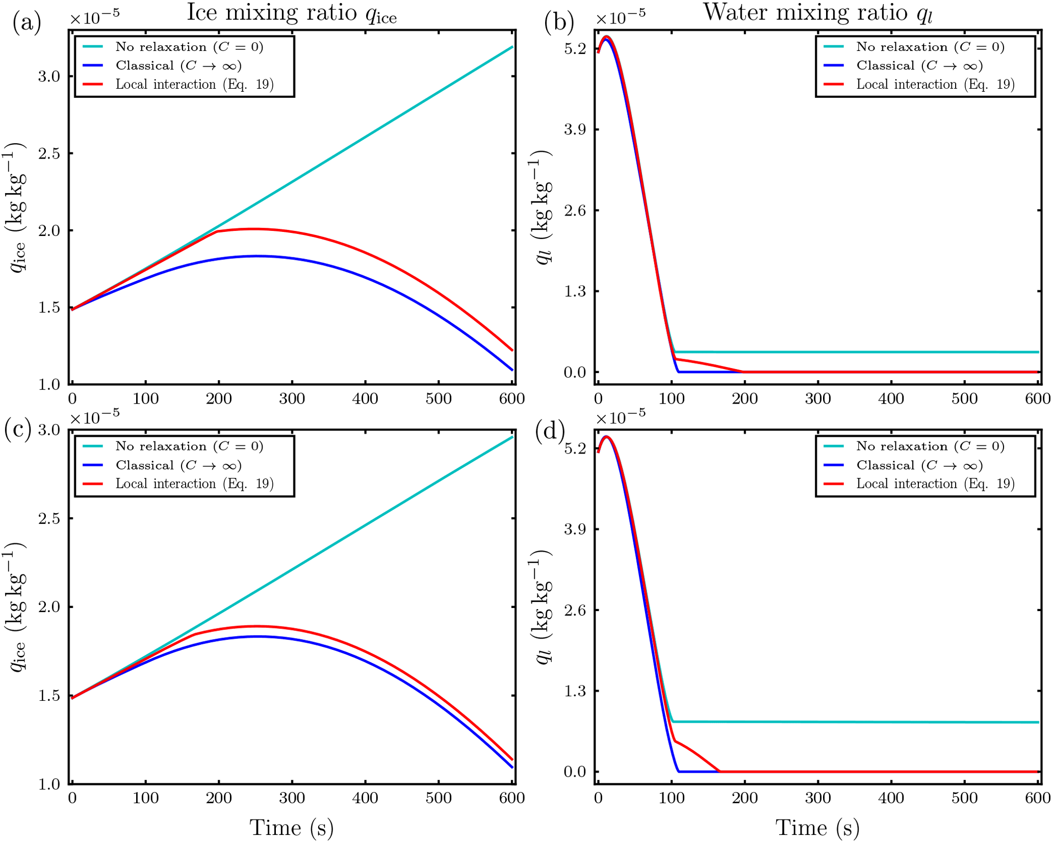
https://www.atmos-chem-phys.net/18/2525/2018/acp-18-2525-2018-f08

Figure 8Temporal evolution of the ice mixing ratio in panels (a) and (c) and the liquid water mixing ratio in panels (b) and (d) for the parcel model simulations with $w = - 1 m s^{- 1}$ at initial ambient saturation ratio S_∞=1.01. Panels (a) and (b) show the case with N_d=200 droplets in each influence sphere of the ice crystals and droplet distance l₀=5R_i. Panels (c) and (d) show the case with N_d=500 and droplet distance l₀=30R_i. Note the different scaling of the axes.

Download

https://www.atmos-chem-phys.net/18/2525/2018/acp-18-2525-2018-f09

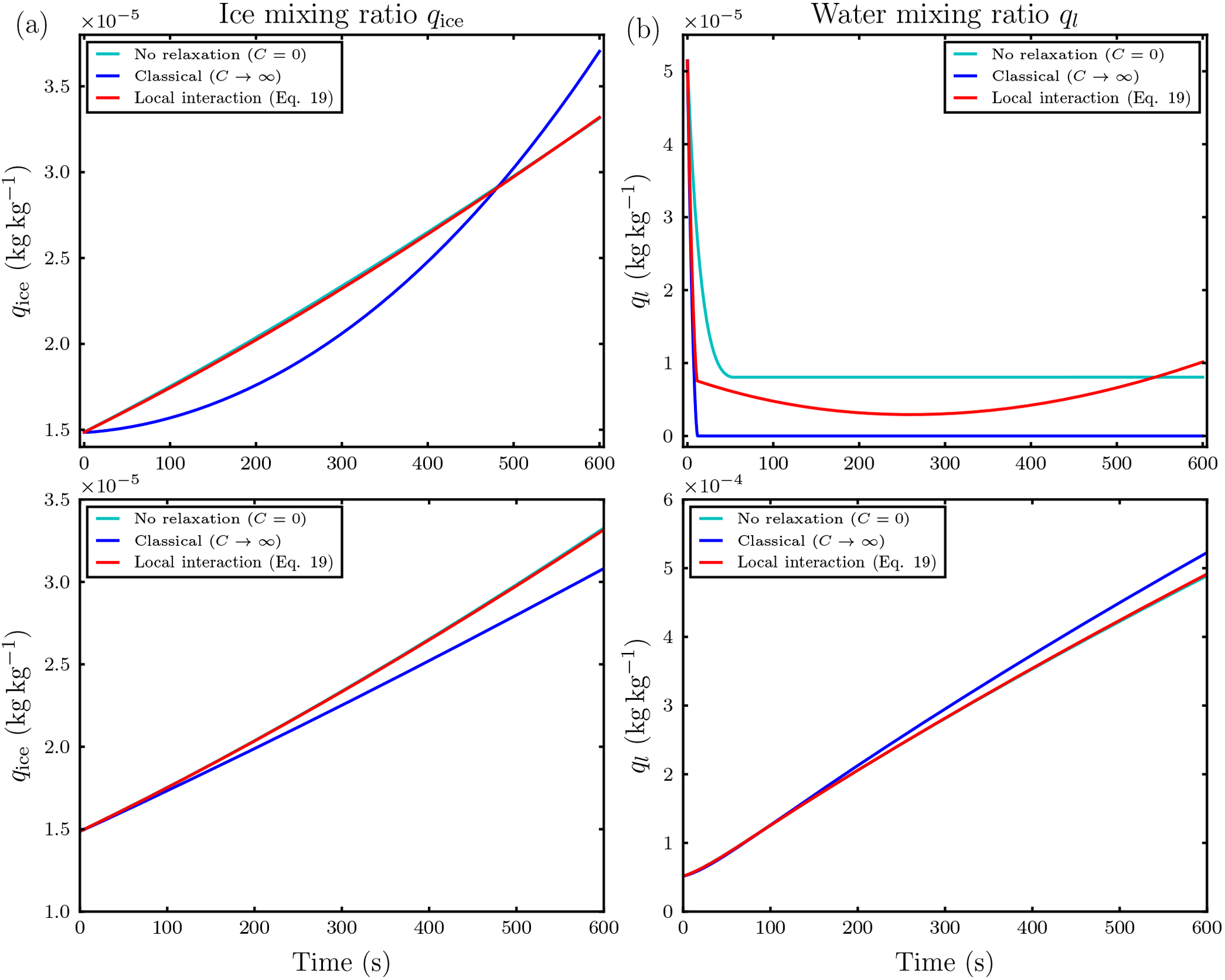
Figure 9Temporal evolution of the ice mixing ratio (a) and liquid water mixing ratio (b) for the parcel model simulation with $w = 1, m s^{- 1}$ and N_d=500 droplets in each influence sphere of the ice crystals and droplet distance l₀=5R_i. The upper row is at ambient saturation ratio S_∞=0.847 and the lower row is at S_∞=1.01. Note the different scaling of the axes.

Download

3.2.2 Vertical velocity $w = - 1 m s^{- 1}$

In a descending air parcel, the saturation ratio decreases monotonically due to the adiabatic heating, causing an initially supersaturated air parcel to become subsaturated after a short time. According to the discussion in the previous subsection, we expect only a negligible influence of the local effects on the temperature T_∞ of the air parcel. This was confirmed by our conducted simulations.

Contrary to the case of vanishing vertical velocity discussed in the previous subsection, local effects are clearly visible in the mixing ratios for an initially supersaturated air parcel. In the following, we show two examples, the first with a small droplet–ice distance and droplet number and the second with an increased droplet–ice distance and droplet number.

As the first example we choose a droplet–ice distance l₀=5R_i, droplet number N_d=200 and initial ambient saturation ratio S_∞=1.01. The temporal evolution of the mixing ratios is shown in Fig. 8a and b. From the ice mixing ratio curve in Fig. 8a it is evident that ice crystals evaporate much slower in comparison with the classical case without local interactions (blue curve). Also the droplets inside the influence spheres of ice crystals can exist longer compared to the classical case; see Fig. 8b. The droplets inside the influence sphere evaporate slower because their released water vapor raises the local coupling value $ρ_{v, *}$ and consequently slows down further evaporation. This explains the first kink at about t=105 s of the red curve in Fig. 8b, in which all outer droplets are evaporated. The second kink at about t=197 s marks the complete evaporation of all droplets. In this example, the droplets in the influence sphere exist up to 100 s longer than the droplets outside. As is indicated by the cyan curve, the time span may even be longer if the local relaxation rate C is smaller. From Fig. 8a we additionally observe that the red curve for the ice mixing ratio does not deviate significantly from the extreme case without local relaxation (cyan curve) until all droplets in the air parcel are evaporated (at about t=197 s). Therefore, a smaller local relaxation rate increases the time until the red curve deviates from the cyan curve.

In the second example with a moderate droplet–ice distance l₀=30R_i, ambient saturation ratio S_∞=1.01 and N_d=500 droplets, we observe similar effects as before; see Fig. 8c and d. Using the larger droplet–ice distance it is important to have more droplets inside the influence spheres to compensate for the larger distance in order to observe a similar effect of the local interactions. In this case, the delay in the complete evaporation of the droplets inside the influence spheres is about 50 s; see Fig. 8d, in which the first kink is at about t=105 s and the second kink at about t=166 s.

The longest delay of about 180 s in the evaporation of the droplets was found in the simulations using the small droplet–ice distance l₀=5R_i and initial saturation ratios $S_{\infty} \in {0.932, 1.01}$ (not shown).

3.2.3 Vertical velocity $w = 1 m s^{- 1}$

https://www.atmos-chem-phys.net/18/2525/2018/acp-18-2525-2018-f10

Figure 10Temporal evolution of saturation ratio S_∞ with respect to water for the same simulation as in the upper row of Fig. 9 with ambient saturation ratio S_∞=0.847.

Download

https://www.atmos-chem-phys.net/18/2525/2018/acp-18-2525-2018-f11

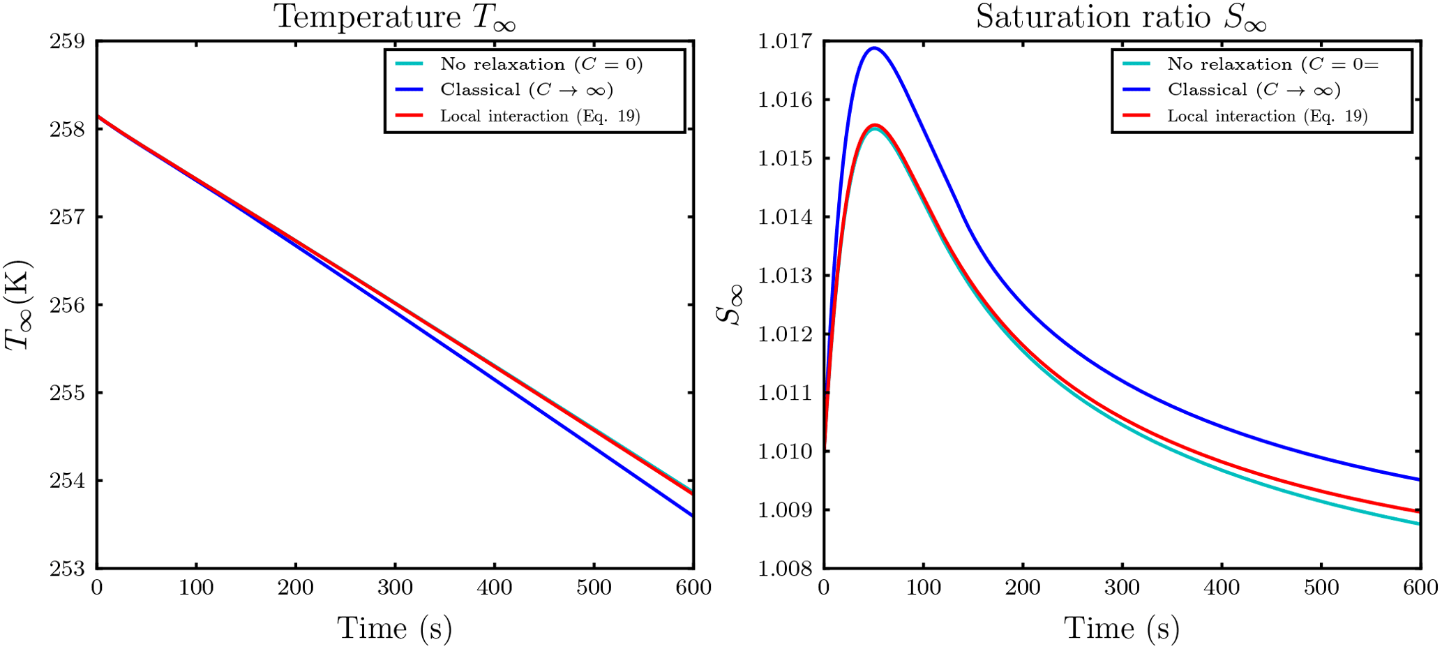
Figure 11Temporal evolution of air parcel temperature T_∞ and saturation ratio S_∞ with respect to water for the same simulation as in the lower row in Fig. 9 with droplet distance l₀=5R_i.

Download

For updrafts, a significant effect of local interactions on the mixing ratios was not observed in our conducted simulations. Even in a massively water subsaturated regime S_∞=0.847 with small droplet–ice distance l₀=5R_i and high droplet number N_d=500, in which we expect the largest effect of the local interactions, an effect of the local interactions on the ice mixing ratio was only minor; see the upper left panel in Fig. 9. Because of the ascent, the air parcel cools and the saturation ratio increases. Remarkably in this simulation, the droplets inside the influence spheres of the ice crystals managed to survive the time span until the air parcel became saturated, whereas all droplets outside the influence spheres and in the classical treatment without the local interactions evaporated earlier; see the upper right panel in Fig. 9. The air parcel became saturated with respect to water at about 200 s; see Fig. 10. From the same figure it is evident that the saturation ratio increased towards unrealistically high values of about 10 % after 350 s because we neglected the activation of new droplets in our simulations. In reality, such high supersaturations are efficiently removed by the activation and further diffusional growth of new droplets (Lamb and Verlinde, 2011).

However, considering only the simulations in which the saturation ratio stayed within a reasonable realistic range, we show as an example the case with initial water supersaturation and saturation ratio S_∞=1.01, droplet distance l₀=5R_i and N_d=500 droplets per influence sphere. The temporal evolution of the mixing ratios is shown in the lower row in Fig. 9. Compared to the classical case, the ice growth rate is slightly increased. This increase is sufficient to raise the temperature T_∞ of the air parcel by approximately 0.25 K over the classical case; see the left panel in Fig. 11. The right panel in this figure confirms that the ambient saturation ratio stayed within a realistic range. From all conducted simulations with vertical velocity $w = 1 m s^{- 1}$ , this was the most pronounced effect on air parcel temperature.

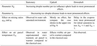
Table 2Summary of the observed effects within the conducted air parcel simulations.

Download Print Version | Download XLSX

4 Conclusions

In this study, we considered the modeling of local interactions between hydrometeors, specifically the case of an ice crystal and surrounding cloud droplets. We were interested in capturing the impact of locality on the diffusional growth of the hydrometeors. In contrast to the study by Baumgartner and Spichtinger (2017), we suggested a formulation of the local interaction that may be suited to incorporate into a bulk microphysics model. Since this formulation allows for a more physically consistent representation of the interaction between ice crystals and cloud droplets, the model may improve the representation of the Wegener–Bergeron–Findeisen process. Apart from the derivation of the model, we incorporated the suggested model into an air parcel framework in order to assess the impact of local interactions on a mixed-phase cloud.

A summary of the observed effects and trends within our conducted simulations is given in Table 2. The dependence on the system parameters N_d and l₀, documented in the first two rows of Table 2, was to be expected by construction of the model in Sect. 2 and is independent of the choice of the other parameters. All simulations were carried out with initial radius R_i=100 µm for the ice crystal and r_d=10 µm for the cloud droplets. Other choices for the initial radii will modify the rate of change in the mass of the hydrometeors and therefore the overall intensity and duration of local effects but not the qualitative influence of the parameters N_d and l₀.

The effect of the local interactions is primarily controlled by the droplet–ice distance and the number of droplets in the influence spheres of the ice crystals. An enhancement of the local effects on the mixing ratios is possible through a descending air parcel being initially close to saturation or supersaturated with respect to water. This conclusion is consistent with the theoretical study of Korolev (2008). In this study, various growth regimes of hydrometeors in a mixed-phase cloud were identified and connected to vertical velocities. In order to identify the different regimes, we also employed a parcel model with monodisperse size distributions of the hydrometeors, but excluded local interactions. It was shown that the Wegener–Bergeron–Findeisen process is only active in downdrafts and has its maximal efficiency for vertical velocities around $w = 0 m s^{- 1}$ . Although these findings were obtained with an idealized air parcel model, they seem to be valid in general because similar observations were made in large-eddy simulations of real clouds (Fan et al., 2011).

The heating of the air parcel through local interactions observed in our study is due to an enhanced growth rate of the ice crystals, and therefore the strength of the temperature effect additionally depends on the number of ice crystals inside the air parcel. As detailed before, the ice crystal growth rate also depends on the number N_d of droplets inside the influence spheres and the droplet–ice distance l₀. If the air parcel has a non-vanishing vertical velocity, local interactions may influence the air parcel temperature only in the case of an ascending parcel for high droplet numbers inside the influence spheres and small droplet–ice distances.

One may speculate about the influence of a temperature change in the air parcel on its buoyancy, which depends directly on the temperature of the parcel (Rogers and Yau, 1989). An additional heating of an air parcel with zero vertical velocity may trigger a vertical motion in an unstable stratification.

Although air parcel models are widely used, they might overestimate or underestimate the strength of observed effects. Therefore one should include the suggested local interaction model into a large-eddy model framework and again analyze the influence of the local interactions seen in this study with the more realistic model, which is left for future work.

In this study we only considered local interactions regarding the diffusional growth of the ice crystal and surrounding cloud droplets. Another aspect of hydrometeors with only small distances is an enhanced collision probability. It is known that small-scale turbulence enhances collision probability. In our context, an enhanced collision probability means an enhanced probability for riming of the ice crystals. In addition, the observed delays in the evaporation of the cloud droplets may also contribute to an increase in riming efficiencies.

Data availability

The data of this study are available from the corresponding author upon request.

Appendix A

https://www.atmos-chem-phys.net/18/2525/2018/acp-18-2525-2018-f12

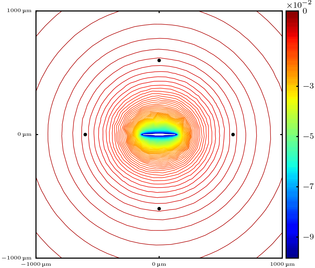
Figure A1Contour lines of the supersaturation with respect to water around the ice crystal at time instant 5 s. Although the computational domain is a cuboid with edge length 6000 µm, the figure shows only a reduced cuboid with edge length 2000 µm centered around the ice crystal. The black dots show the positions of the droplets with coordinates $(\pm 600 µ m, 0, 0)$ and $(0, \pm 600 µ m, 0)$ .

Download

In this appendix, we show an example of the effect of ice crystal shape on the diffusional growth behavior of surrounding droplets by using the reference model described in Baumgartner and Spichtinger (2017). The model is a direct numerical simulation model and resolves the involved hydrometeors as well as the water vapor and temperature field. We simulate a case as depicted in the schematic Fig. 2 in which the ice crystal now has an ellipsoidal shape with a major axis length 150 µm and minor axis length 10 µm. The ice crystal is placed in the center of a cubic computational domain with edge length 6000 µm. We place 38 droplets with radius 10 µm along the Lebedev quadrature points (Lebedev, 1976) and distance $R_{*} = 600 µ m$ , matching the case l₀=5R_i used in the air parcel simulations in Sect. 3.2. The simulation time is 5 s. Figure A1 shows the contour lines of supersaturation with respect to water along a slice at height z=0 through the computational domain. It is seen that the ice crystal is visible as a strong sink for water vapor, but the contour lines appear as almost spherical at some distance from the ice crystal.

Figure A2 shows the temporal evolution of the droplet masses. In Fig. A2a, the corresponding curves of all 38 droplets are shown and a different growth behavior is obvious. In Fig. A2b, only the temporal evolution of the four marked droplets in Fig. A1 is shown. The droplets with coordinates $(\pm 600 µ m, 0, 0)$ are closest to the ice crystal and evaporate (red curves), while the droplets with coordinates $(0, \pm 600 µ m, 0)$ have the largest distance from the ice crystal surface and grow (blue curves); i.e., they show different growth behavior. According to these considerations it is obvious that including this effect requires precise information not only about the shape of the ice crystal but also about the relative positions of the droplets with respect to the ice crystal surface. Such information is not available in numerical models and therefore we neglect this dependence.

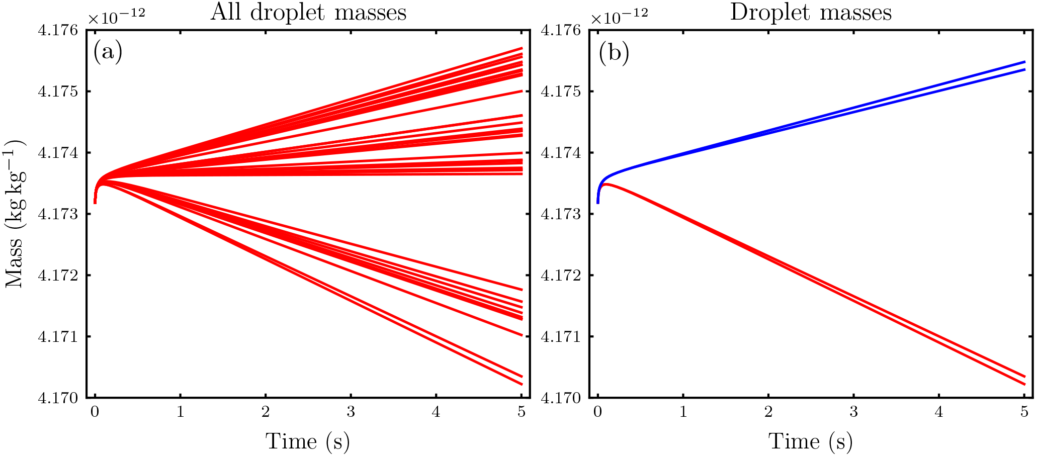
https://www.atmos-chem-phys.net/18/2525/2018/acp-18-2525-2018-f13

Figure A2Temporal evolution of the droplet masses. (a) The droplet masses of all 38 droplets and (b) the droplet masses of the droplets with coordinates $(\pm 600 µ m, 0, 0)$ (red curves) and $(0, \pm 600 µ m, 0)$ (blue curves).

Download

Appendix B

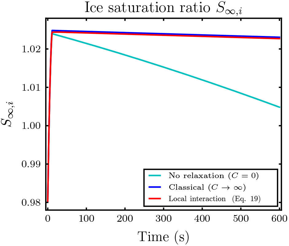
Figure B1 shows the temporal evolution of the saturation ratio S_∞,i with respect to ice for the first simulation in Sect. 3.2.1 with vanishing velocity, N_d=40 droplets per ice crystal influence sphere and droplet distance l₀=5R_i. Although the air parcel is initially subsaturated with respect to ice, the evaporating droplets release enough water vapor to the air parcel to cause an ice supersaturated environment.

https://www.atmos-chem-phys.net/18/2525/2018/acp-18-2525-2018-f14

Figure B1Temporal evolution of saturation ratio S_∞,i with respect to ice for the same simulation as in the upper row in Fig. 6.

Download

Competing interests

The authors declare that they have no conflict of interest.

Acknowledgements

We thank A. Seifert for fruitful discussions. This study was prepared with support from the German Bundesministerium für Bildung und Forschung (BMBF) within the HD(CP)² initiative, project M6 (001LK1207A) and the Deutsche Forschungsgemeinschaft (DFG) within the project “Enabling Performance Engineering in Hesse and Rhineland-Palatinate” (grant number 320898076).

Edited by: Athanasios Nenes
Reviewed by: two anonymous referees

References

Baumgartner, M. and Spichtinger, P.: Local Interactions by Diffusion between Mixed-Phase Hydrometeors: Insights from Model Simulations, Mathematics of Climate and Weather Forecasting, 3, 64–89, https://doi.org/10.1515/mcwf-2017-0004, 2017. a, b, c, d, e, f, g

Baumgartner, M. and Spichtinger, P.: Diffusional growth of cloud particles: existence and uniqueness of solutions, Theor. Comp. Fluid Dyn., 32, 47–62, https://doi.org/10.1007/s00162-017-0437-x, 2018. a

Beals, M. J., Fugal, J. P., Shaw, R. A., Lu, J., Spuler, S. M., and Stith, J. L.: Holographic measurements of inhomogeneous cloud mixing at the centimeter scale, Science, 350, 87–90, 2015. a

Bergeron, T.: The Problem of Artificial Control of Rainfall on the Globe, Tellus, 1, 32–43, 1949. a

Castellano, N. E. and Avila, E. E.: Vapour density field of a population of cloud droplets, J. Atmos. Sol.-Terr. Phy., 73, 2423–2428, 2011. a

Celani, A., Falkovich, G., Mazzino, A., and Seminara, A.: Droplet condensation in turbulent flows, EPL (Europhysics Letters), 70, 775–781, 2005. a

Celani, A., Mazzino, A., Seminara, A., and Tizzi, M.: Droplet condensation in two-dimensional Bolgiano turbulence, J. Turbul., 8, 1–9, 2007. a

Chen, J.-P. and Lamb, D.: The Theoretical Basis for the Parameterization of Ice Crystal Habits: Growth by Vapor Deposition, J. Atmos. Sci., 51, 1206–1222, 1994. a

Davis, E.: A history and state-of-the-art of accommodation coefficients, Atmos. Res., 82, 561–578, 2006. a

Devenish, B. J., Bartello, P., Brenguier, J.-L., Collins, L. R., Grabowski, W. W., IJzermans, R. H. A., Malinowski, S. P., Reeks, M. W., Vassilicos, J. C., Wang, L.-P., and Warhaft, Z.: Droplet growth in warm turbulent clouds, Q. J. Roy. Meteor. Soc., 138, 1401–1429, 2012. a

Fan, J., Ghan, S., Ovchinnikov, M., Liu, X., Rasch, P. J., and Korolev, A. V.: Representation of Arctic mixed-phase clouds and the Wegener-Bergeron-Findeisen process in climate models: Perspectives from a cloud-resolving study, J. Geophys. Res.-Atmos., 116, 1–17, 2011. a

Findeisen, W.: Die Kolloidmeteorologischen Vorgänge bei der Niederschlagsbildung, Meteor. Z., 55, 121–133, 1938. a

Fleishauer, R. P., Larson, V. E., and Haar, T. H. V.: Observed Microphysical Structure of Midlevel, Mixed-Phase Clouds, J. Atmos. Sci., 59, 1779–1804, 2002. a, b

Fugal, J. P. and Shaw, R. A.: Cloud particle size distributions measured with an airborne digital in-line holographic instrument, Atmos. Meas. Tech., 2, 259-271, https://doi.org/10.5194/amt-2-259-2009, 2009. a

Grabowski, W. W. and Wang, L.-P.: Growth of Cloud Droplets in a Turbulent Environment, Annu. Rev. Fluid Mech., 45, 293–324, 2013. a

Hobbs, P. V., Rangno, A. L., Shupe, M., and Uttal, T.: Airborne Studies of Cloud Structures over the Arctic Ocean and Comparisons with Retrievals from Ship-Based Remote Sensing Measurements, J. Geophys. Res.-Atmos., 106, 15029–15044, 2001. a

Korolev, A. V.: Rates of phase transformations in mixed-phase clouds, Q. J. Roy. Meteor. Soc., 134, 595–608, 2008. a

Korolev, A. V., Isaac, G. A., Cober, S. G., Strapp, J. W., and Hallett, J.: Microphysical characterization of mixed-phase clouds, Q. J. Roy. Meteor. Soc., 129, 39–65, 2003. a, b, c

Kostinski, A. B. and Shaw, R. A.: Scale-dependent droplet clustering in turbulent clouds, J. Fluid Mech., 434, 389–398, 2001. a

Lamb, D. and Verlinde, J.: Physics and Chemistry of Clouds, Cambridge University Press, Cambridge, 2011. a, b, c, d, e, f

Lebedev, V.: Quadratures on a sphere, USSR Comp. Math. Math.+, 16, 10–24, 1976. a, b

Lloyd, G., Choularton, T. W., Bower, K. N., Gallagher, M. W., Connolly, P. J., Flynn, M., Farrington, R., Crosier, J., Schlenczek, O., Fugal, J., and Henneberger, J.: The origins of ice crystals measured in mixed-phase clouds at the high-alpine site Jungfraujoch, Atmos. Chem. Phys., 15, 12953–12969, https://doi.org/10.5194/acp-15-12953-2015, 2015. a

Marshall, J. S. and Langleben, M. P.: A Theory of Snow-Crystal Habit and Growth, J. Meteorol., 11, 104–120, 1954. a

Maxwell, J. C.: Diffusion, in: The Scientific Papers of James Clerk Maxwell, edited by: Niven, W. D., Dover Publications, Inc., New York, 2, 625–645, 1877. a

Noh, Y.-J., Seaman, C. J., Haar, T. H. V., and Liu, G.: In Situ Aircraft Measurements of the Vertical Distribution of Liquid and Ice Water Content in Midlatitude Mixed-Phase Clouds, J. Appl. Meteorol. Clim., 52, 269–279, 2013. a

Pinto, J. O., Curry, J. A., and Intrieri, J. M.: Cloud-aerosol interactions during autumn over Beaufort Sea, J. Geophys. Res.-Atmos., 106, 15077–15097, 2001. a

Pruppacher, H. R. and Klett, J. D.: Microphysics of Clouds and Precipitation, vol. 18 of Atmospheric and Oceanographic Sciences Library, Kluwer Academic Publishers, Dordrecht, second revised and enlarged edition, 1997. a

Reiss, H.: The Growth of Uniform Colloidal Dispersions, J. Chem. Phys., 19, 482–487, 1951. a

Reiss, H. and La Mer, V. K.: Diffusional Boundary Value Problems Involving Moving Boundaries, Connected with the Growth of Colloidal Particles, J. Chem. Phys., 18, 1–12, 1950. a

Rogers, R. and Yau, M.: A Short Course in Cloud Physics, International Series in Natural Philosophy, Butterworth-Heinemann, third edition edn., 1989. a, b, c

Schlenczek, O., Fugal, J. P., Lloyd, G., Bower, K. N., Choularton, T. W., Flynn, M., Crosier, J., and Borrmann, S.: Microphysical Properties of Ice Crystal Precipitation and Surface-Generated Ice Crystals in a High Alpine Environment in Switzerland, J. Appl. Meteorol. Clim., 56, 433–453, 2017. a

Shaw, R. A., Reade, W. C., Collins, L. R., and Verlinde, J.: Preferential Concentration of Cloud Droplets by Turbulence: Effects on the Early Evolution of Cumulus Cloud Droplet Spectra, J. Atmos. Sci., 55, 1965–1976, 1998. a

Srivastava, R. C.: Growth Of Cloud Drops by Condensation: A Criticism of Currently Accepted Theory and a New Approach, J. Atmos. Sci., 46, 869–887, 1989. a

Vaillancourt, P. A. and Yau, M. K.: Review of Particle-Turbulence Interactions and Consequences for Cloud Physics, B. Am. Meteorol. Soc., 81, 285–298, 2000. a

Vaillancourt, P. A., Yau, M. K., and Grabowski, W. W.: Microscopic Approach to Cloud Droplet Growth by Condensation. Part I: Model Description and Results without Turbulence, J. Atmos. Sci., 58, 1945–1964, 2001. a

Vaillancourt, P. A., Yau, M. K., Bartello, P., and Grabowski, W. W.: Microscopic Approach to Cloud Droplet Growth by Condensation. Part II: Turbulence, Clustering, and Condensational Growth, J. Atmos. Sci., 59, 3421–3435, 2002. a

Verlinde, J., Harrington, J. Y., Yannuzzi, V. T., Avramov, A., Greenberg, S., Richardson, S. J., Bahrmann, C. P., McFarquhar, G. M., Zhang, G., Johnson, N., Poellot, M. R., Mather, J. H., Turner, D. D., Eloranta, E. W., Tobin, D. C., Holz, R., Zak, B. D., Ivey, M. D., Prenni, A. J., DeMott, P. J., Daniel, J. S., Kok, G. L., Sassen, K., Spangenberg, D., Minnis, P., Tooman, T. P., Shupe, M., Heymsfield, A. J., and Schofield, R.: The Mixed-Phase Arctic Cloud Experiment, B. Am. Meteorol. Soc., 88, 205–221, 2007. a

Wang, P. K.: Physics and Dynamics of Clouds and Precipitation, Cambridge University Press, Cambridge, 2013. a, b

Wegener, A.: Thermodynamik der Atmosphäre, J. A. Barth, Leipzig, 1911. a

Wood, A., Hwang, W., and Eaton, J.: Preferential concentration of particles in homogeneous and isotropic turbulence, Int. J. Multiphas. Flow, 31, 1220–1230, 2005. a

Zhao, Z. and Lei, H.: Aircraft observations of liquid and ice in midlatitude mixed-phase clouds, Adv. Atmos. Sci., 31, 604–610, 2014. a, b

Articles

Short summary

Ice crystals are surrounded by liquid cloud droplets in mixed-phase clouds. The coexistence of ice and water is thermodynamically not stable and the particles will influence their respective growth by condensation. This effect is known as the Wegener–Bergeron–Findeisen process. In current models, the local interactions of the particles are neglected and they can only interact indirectly. This work proposes an approach to include local interactions and discusses some implications.

Towards a bulk approach to local interactions of hydrometeors

2.1 Local ice–droplet system

2.1.1 Description

2.1.2 Derivation

2.2 Choice of parameters

2.2.1 Parameter for droplet distance

2.2.2 Parameter for radii of the influence spheres

2.2.3 Number parameter

2.2.4 Distribution parameter

2.3 Simplifications

2.4 Discussion of the model ansatz

3.1 Description of the parcel model

3.2 Results

3.2.1 Vertical velocity w=0ms-1

3.2.2 Vertical velocity w=-1ms-1

3.2.3 Vertical velocity w=1ms-1

3.2.1 Vertical velocity $w = 0 m s^{- 1}$

3.2.2 Vertical velocity $w = - 1 m s^{- 1}$

3.2.3 Vertical velocity $w = 1 m s^{- 1}$