the Creative Commons Attribution 4.0 License.
the Creative Commons Attribution 4.0 License.
 | 21 Dec 2018
Attribution of recent increases in atmospheric methane through 3-D inverse modelling
Joe McNorton
Chris Wilson
Manuel Gloor
Rob J. Parker
Hartmut Boesch
Wuhu Feng
Ryan Hossaini
Martyn P. Chipperfield
The atmospheric methane (CH4) growth rate has varied considerably in recent decades. Unexplained renewed growth after 2006 followed 7 years of stagnation and coincided with an isotopic trend toward CH4 more depleted in 13C, suggesting changes in sources and/or sinks. Using surface observations of both CH4 and the relative change of isotopologue ratio (δ13CH4) to constrain a global 3-D chemical transport model (CTM), we have performed a synthesis inversion for source and sink attribution. Our method extends on previous studies by providing monthly and regional attribution of emissions from six different sectors and changes in atmospheric sinks for the extended 2003–2015 period. Regional evaluation of the model CH4 tracer with independent column observations from the Greenhouse Gases Observing Satellite (GOSAT) shows improved performance when using posterior fluxes (R=0.94–0.96, RMSE =8.3–16.5 ppb), relative to prior fluxes (R=0.60–0.92, RMSE =48.6–64.6 ppb). Further independent validation with data from the Total Carbon Column Observing Network (TCCON) shows a similar improvement in the posterior fluxes (R=0.87, RMSE =18.8 ppb) compared to the prior fluxes (R=0.69, RMSE =55.9 ppb). Based on these improved posterior fluxes, the inversion results suggest the most likely cause of the renewed methane growth is a post-2007 1.8±0.4 % decrease in mean OH, a 12.9±2.7 % increase in energy sector emissions, mainly from Africa–Middle East and southern Asia–Oceania, and a 2.6±1.8 % increase in wetland emissions, mainly from northern Eurasia. The posterior wetland flux increases are in general agreement with bottom-up estimates, but the energy sector growth is greater than estimated by bottom-up methods. The model results are consistent across a range of sensitivity analyses. When forced to assume a constant (annually repeating) OH distribution, the inversion requires a greater increase in energy sector (13.6±2.7 %) and wetland (3.6±1.8 %) emissions and an 11.5±3.8 % decrease in biomass burning emissions. Assuming no prior trend in sources and sinks slightly reduces the posterior growth rate in energy sector and wetland emissions and further increases the magnitude of the negative OH trend. We find that possible tropospheric Cl variations do not influence δ13CH4 and CH4 trends, although we suggest further work on Cl variability is required to fully diagnose this contribution. While the study provides quantitative insight into possible emissions variations which may explain the observed trends, uncertainty in prior source and sink estimates and a paucity of δ13CH4 observations limit the robustness of the posterior estimates.
- Article
(9428 KB) - Full-text XML
- BibTeX
- EndNote


The atmospheric concentration of methane (CH4) has been increasing globally since 2007, following a slowdown in growth from 1999 to 2006 (Dlugokencky et al., 2017). The onset of the observed increase in CH4 coincides with an isotopic trend to lighter CH4, more depleted in 13C (Nisbet et al., 2014). The 13CH4 : 12CH4 ratio (denoted by the δ13CH4 value) is controlled by both the isotopic signatures of the sources and the isotopic fractionation associated with atmospheric CH4 sinks. Broadly speaking, the emissions types can be categorised into the relatively light biogenics ( ‰), heavier fossil fuels ( ‰), and the even heavier biomass burning emissions ( ‰) (Schwietzke et al., 2016), resulting in a total isotopic source signature of between −51 ‰ and −53 ‰. Isotopic fractionation in the atmosphere by the reaction with the hydroxyl (OH) radical and chlorine (Cl) atoms enriches 13CH4, causing a background atmospheric δ13CH4 of ‰.
Previous studies have used simple global box models for source and sink attribution of recent atmospheric CH4 trends, with contradictory findings. Nisbet et al. (2014, 2016) and Schaefer et al. (2016) suggested that either increased wetland or agricultural emissions were the likely cause, while Rigby et al. (2017) and Turner et al. (2017) found the most likely explanation to be a decreased global mean OH concentration. The latter two studies emphasised that the problem is not very well constrained by existing data and as a result could not discard the hypothesis that OH is not changing. These approaches are able to isolate the three emissions categories noted above, and sometimes sink terms. Specific attribution, for example between wetlands and agricultural emissions changes, requires spatial representation of both CH4 and δ13CH4. The box model approach provides little or no information of spatial variation in posterior emissions estimates, preventing regional attribution. Rice et al. (2016) performed a 3-D chemical transport model (CTM) inversion using CH4 and isotopologue measurements over the period from 1984 to 2009. They found a 24 Tg yr−1 increase in fugitive fossil fuel emissions between 1984 and 2009, most of which occurred after 2000. The time trend in their inversion appeared similar to their prior emissions estimates. Although they used a 3-D CTM the posterior emissions were calculated globally and not regionally. Furthermore, their study did not focus on the possible role of OH variations and did not consider inversions after 2009, so only captured 2 years of the continued post-2007 growth.
Here we perform a synthesis inversion using the TOMCAT 3-D CTM, building on previous work (Bousquet et al., 2006, 2011; Rigby et al., 2012; Schwietzke et al., 2016; Rice et al., 2016) and using surface measurements of both CH4 (Dlugokencky et al., 2017) and δ13CH4 (White et al., 2017). The synthesis inversion technique uses the forward 3-D CTM to optimise monthly CH4 emissions over relatively large regions and for multiple source sectors. This spatial resolution is not present in existing box model inversions. We investigate regional source contributions and the roles of tropospheric OH and Cl in the recent growth of CH4. From this we derive possible source and sink changes between 2003 and 2015 which best fit the observations.
2.1 Chemical transport model
2.1.1 Forward model
The TOMCAT global CTM (Chipperfield et al., 2006) has previously been widely used to simulate CH4 trends and has been evaluated against observations (e.g. Patra et al., 2011; Wilson et al., 2016; Parker et al., 2018). Here we base our synthesis inversions on TOMCAT simulations at resolution with 60 vertical levels from the surface to 60 km for 2003–2015. The simulations used meteorological forcing data from the 6-hourly European Centre for Medium-Range Weather Forecasts ERA-Interim reanalyses (Dee et al., 2011). The model was spun up from a 1977 initialisation field before the mean global CH4 and δ13CH4 were rescaled to match NOAA observations in January 2002. A 1-year inversion spin-up was then performed for 2002 to optimise the 3-D CH4 and δ13CH4 concentration fields relative to observations, and the results shown here begin in January 2003.
Monthly varying methane emissions from McNorton et al. (2016a) were updated using revisions based on those of Schwietzke et al. (2016), which increased fossil fuel emissions and decreased biogenic emissions compared to the estimates in Saunois et al. (2016). OH and stratospheric CH4 loss fields were taken from McNorton et al. (2016b), and a TOMCAT-derived tropospheric Cl loss field (Hossaini et al., 2016) was applied for the first time in our model.
Table 1Source and sink isotope signatures used in the TOMCAT 3-D CTM. Values for prior emissions (Kirschke et al., 2013; McNorton et al., 2016a; Schwietzke et al., 2016) and isotope signatures (Saueressig et al., 2001; Mikaloff-Fletcher et al., 2004; Feilberg et al., 2005; Whiticar et al., 2007; Schwietzke et al., 2016) are based on previous studies. Note that the soil sink is not optimised and modelled as a negative emission. Posterior emissions estimates are shown with posterior error estimates.
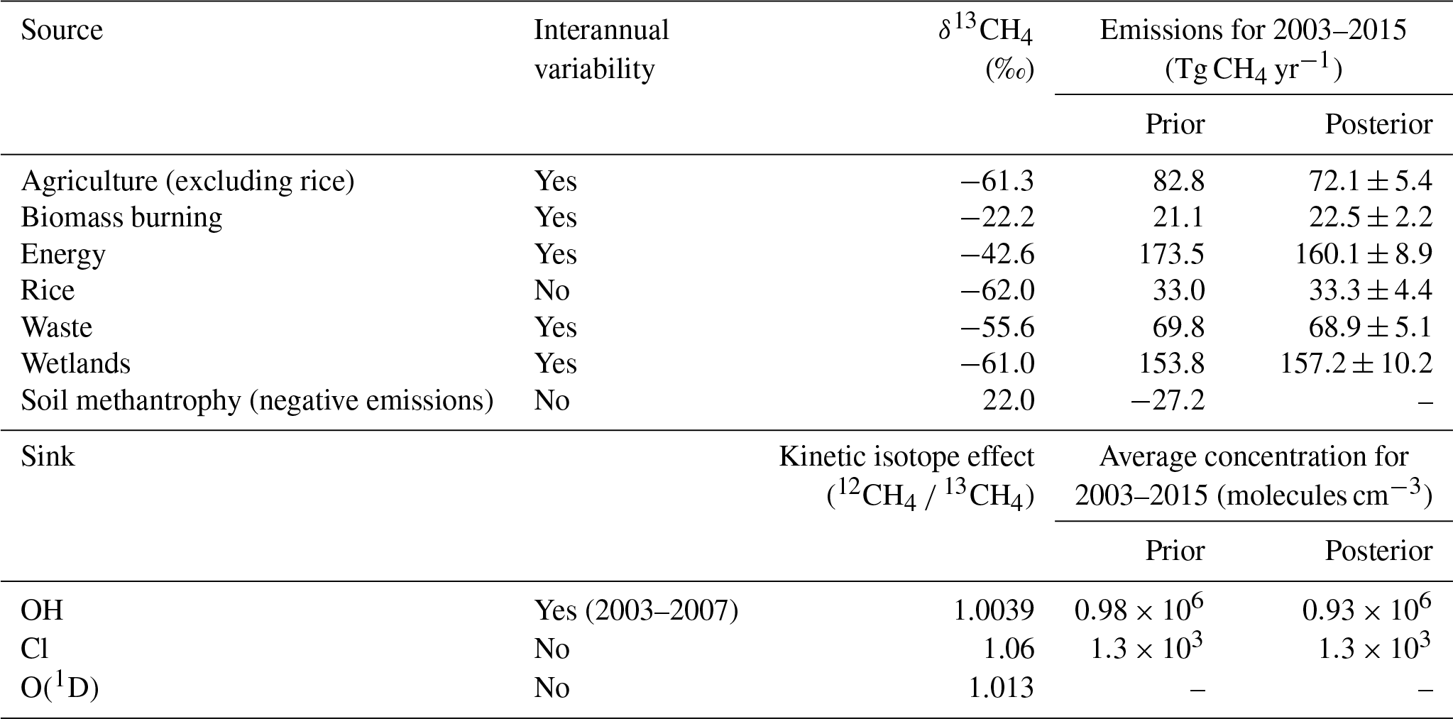
Emissions were grouped into individual tracers for agriculture (excluding rice), biomass burning, energy, rice, waste, wetlands, and “supplementary”, made up of the remaining sources (geological, hydrates, oceans, and termites). Each source type, excluding supplementary, was then sub-divided into five geographic regions: North America (NA), northern Eurasia (EA), South America (SA), Africa and the Middle East (AM), and South Asia and Oceania (AO) (see Fig. 7). These regions were chosen by grouping existing Transcom regions (DeFries et al., 1994) and considering both socio-economic and biome similarities. The aggregation of regions by combining both socio-economic and biome considerations is somewhat subjective and differing aggregations may influence synthesis inversion results (Kaminski et al., 2001), which represents a limitation of the inversion method used in this study. For example, there are socio-economic differences within the EA region, which may result in differing trends in anthropogenic emissions that cannot be resolved using the chosen aggregation; however, biome similarities inside the region mean that the aggregation is appropriate for natural fluxes. We split the Asian regions to derive suitable posterior estimates for boreal and temperate wetlands (EO) and tropical wetlands (AO), for example, although this may affect the posterior energy sector emissions for these regions. Increasing the number of regions would decrease the influence of the aggregation method; however, the computational cost of simulating the tracers required for the synthesis inversion for different sectors and for 12 months effectively limits the number of possible regions that we could use to five.
To assess monthly emissions variability, individual tracers were simulated for each month of the year, excluding supplementary emissions, which were simulated annually. Emissions were further split into separate 12CH4 and 13CH4 tracers using isotopic source signatures taken from Schwietzke et al. (2016) (Table 1), resulting in six source types over five regions for 12 months and two isotopologues, with an additional five regions for supplementary sources (a total of 730 tracers). Kinetic fractionation (Table 1) was accounted for in the atmospheric loss of 13CH4. The simulated tracers were then used to calculate CH4 concentration and δ13CH4 values. To investigate sensitivity to OH and Cl variations, three additional simulations were performed, a control, an OH-enhanced simulation (1 % increase), and a tropospheric Cl-enhanced simulation (1 % increase). Any feedback on the CH4 term within the loss rate from the small adjustments made (1 %) is assumed to be negligible.
2.1.2 Synthesis inversion
Our global synthesis inversions build on techniques used in Bousquet et al. (2006), Bergamaschi et al. (2007), and Rigby et al. (2012). Prior estimates of sources and sinks, uncertainty estimates, and observations of both CH4 and δ13CH4 were used to quantify posterior estimates of sources and sinks. Posterior estimates were then used in a second forward simulation for the same year, which provided an initialisation field for the subsequent year. The inversion method is limited by the assumption that isotopic source signatures are known.
For the inversion including OH concentrations in the state vector we consider the total simulated CH4 mixing ratio (φ) and the δ13CH4 value (ψ) at time, t, at each measurement location, l. These are described as a linear combination of contributions from nreg emissions regions separated into nmonth months and nsource emissions sectors, loss due to OH, fractionation due to OH, the initial mixing ratio at the location, φini, and the initial δ13CH4 value at the location, ψini.
Note that we use Δ here to represent change, to avoid confusion with the isotopologue δ13CH4. Basis functions and are sensitivities of atmospheric CH4 and δ13CH4 at a particular time and location to an emission of 1 Tg of CH4 from a region i during a particular month m, for an emissions sector s. Each is a scaling factor applied to the contribution from each basis function and is initially set equal to the prior value of the emissions. Similarly, and are the sensitivities of the mixing ratio and δ13CH4 at a measurement location to a change in the global OH concentration, linearised around the prior, and xOH is initially set to be the prior OH concentration. xini is a dimensionless scaling factor initially set to be 1. Although the emissions in each region and source type are split into 12CH4 and 13CH4, the relative emissions of each isotopologue from each region for each source type are not included as separate basis functions. The “state vector” x comprises the individual emissions scaling factors , for all i, m, and s values, along with xOH and xini. Sensitivity experiments performed for tropospheric Cl follow the same formulation with Cl terms replacing OH terms.
Varying atmospheric CH4 concentrations in the inversions should in principle result in a non-linear feedback on OH concentration. This feedback is not accounted for in the offline OH field used in our inversion. To resolve this, an online OH field could be used with an iterative minimisation of the cost function. However, Bousquet et al. (2011) found that the small variation in CH4 concentration between the prior and posterior had a negligible influence on OH concentration.
The model OH is constrained by CH4 and δ13CH4 but not by other species, such as methylchloroform (MCF). MCF was excluded because of uncertainty in emissions and a diminishing concentration (<5 ppt), particularly during the later period of the study (Liang et al., 2017). Due to the large uncertainty relative to the observed MCF concentrations in this period, including the extra species within the inversion would not add any extra constraint on the global OH concentration.
Independent inversions (INV-FULL) were performed for each year from 2003 to 2015. Initial conditions for each year are provided by a forward simulation for the previous year driven by derived posterior emissions and loss rates, with 2003 initial conditions taken from a 2002 spin-up inversion. To quantify the optimisation of the flux terms in each region and the sink term, we calculate the cost function, J:
The value of this cost function is dependent on the value of the state vector x. The vector y contains the observations. xb is the a priori estimate of x, and B is the error covariance matrix containing the uncertainties placed on the prior estimates, and the covariances between these uncertainties. G is the sensitivity matrix, which maps x onto the observations, and contains an array made up of the basis functions, and used in Eqs. (1) and (2). R is the diagonal error covariance matrix for the observations and model error.
The minimum of the cost function, which indicates the optimal source–sink scaling, is found using (Tarantola and Valette, 1982)
where xa is the optimised set of scaling factors, which minimise the value of J.
The posteriori error covariance matrix A is calculated from
The initial prior uncertainty of each source within each region was set to 50 %, based on uncertainties given by Kirschke et al., (2013). We assume that increased uncertainty in sources with large interannual variability is offset by those sources having top-down (biomass burning) or process-based (wetlands) interannually varying emissions in our simulations. We assumed small variability in energy sector emissions so assigned a 1-month offset correlation of 0.5; we have not assigned correlations among regions or months in the other prior emissions due to a lack of information. Global annual OH and Cl are assumed to have an uncertainty of 2 %; for OH this is based on estimated interannual variability (Montzka et al., 2011). The impact of varying these uncertainties was investigated. Observational uncertainties were set at 10 ppb for CH4 and 0.1 ‰ for δ13CH4; the increase from the documented uncertainties is to represent model transport uncertainty that would otherwise only be resolved by emissions changes. The magnitude of model transport will vary among different sites; however, as an estimate here we assume all uncertainties to be equal. By separating the inversion into 12-month intervals, the emissions from the previous year are not considered in the inversion for the current year. As a result, December emissions are constrained by fewer observations than January emissions. The influence of this on the posterior error is investigated in Sect. 3.6.
To investigate the effect of including δ13CH4 observations, we performed a separate inversion (INV-CH4) using only CH4 observations. The difference between the inversions indicates the additional information supplied by the inclusion of δ13CH4. Additional sensitivity experiments were also performed, nine with varying prior uncertainties and an additional one with no prior trend in annual emissions, to investigate the robustness of the identified trends from the main inversion.
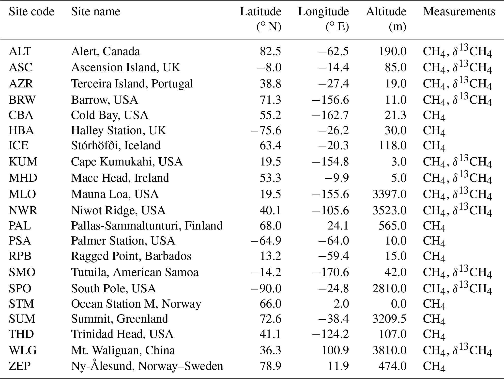
Table 2NOAA measurements from 2003 to 2015 used in the synthesis inversions of CH4 (Dlugokencky et al., 2017) and δ13CH4 (White et al., 2017).
2.2 CH4 and δ13CH4 observations
Monthly mean measurements of CH4 were taken from 21 National Oceanographic and Atmospheric Administration Earth System Research Laboratory (NOAA ESRL) air sampling sites (Dlugokencky et al., 2017) from 2003 to 2015, where available. Measurements of δ13CH4 were taken from 11 NOAA sampling sites and analysed by the Institute of Arctic and Alpine Research (INSTAAR) (White et al., 2017) for the same period (see Table 2). An equal weighting is applied to each monthly mean measurement and potential cross correlations from neighbouring time steps, and spatially nearby sites are not considered.
Column-averaged CH4 (XCH4) GOSAT satellite data provided by the University of Leicester were not included in the inversion but retained for independent validation of the inversion results (Parker et al., 2015). GOSAT was omitted because measurements were only available from 2009, 6 years after the inversion began. The Total Carbon Column Observing Network (TCCON) XCH4 data were used as validation but were considered too intermittent for use in the inversion (Wunch et al., 2011). Finally, two surface observation sites, the High Altitude Global Climate Observation Center (HAGCOC) in Mexico and Cape Grim in Australia, were also used for independent validation.
3.1 Synthesis inversion
Inversion results constrained by CH4 and δ13CH4 observations (INV-FULL) show, as expected, improved seasonal and interannual monthly averaged posterior CH4 and δ13CH4 estimates when compared with assimilated surface observations (Fig. 1). The correlation with observations (R) for CH4 increases from an all-site average of 0.72 in the prior to 0.94 in the posterior, and for δ13CH4 increases from 0.52 to 0.87. Similarly, the root-mean-square error (RMSE) decreases from 38.2 to 9.7 ppb for CH4 and from 0.25 ‰ to 0.09 ‰ for δ13CH4. The prior model captures some of the initial 2007 CH4 growth but fails to capture the sustained growth (Fig. 1a). The bias in the prior, relative to both the posterior and observations, grows throughout the simulation period. This results in a large bias at the end of the time period, which is evident in the large RMSE values (Figs. 1 to 4). The prior also shows a slight decrease in δ13CH4 since 2007, but the magnitude of this is smaller than observed (Fig. 1b). The renewed growth of CH4 and corresponding decrease in δ13CH4 in 2007 are well captured in the inversion.
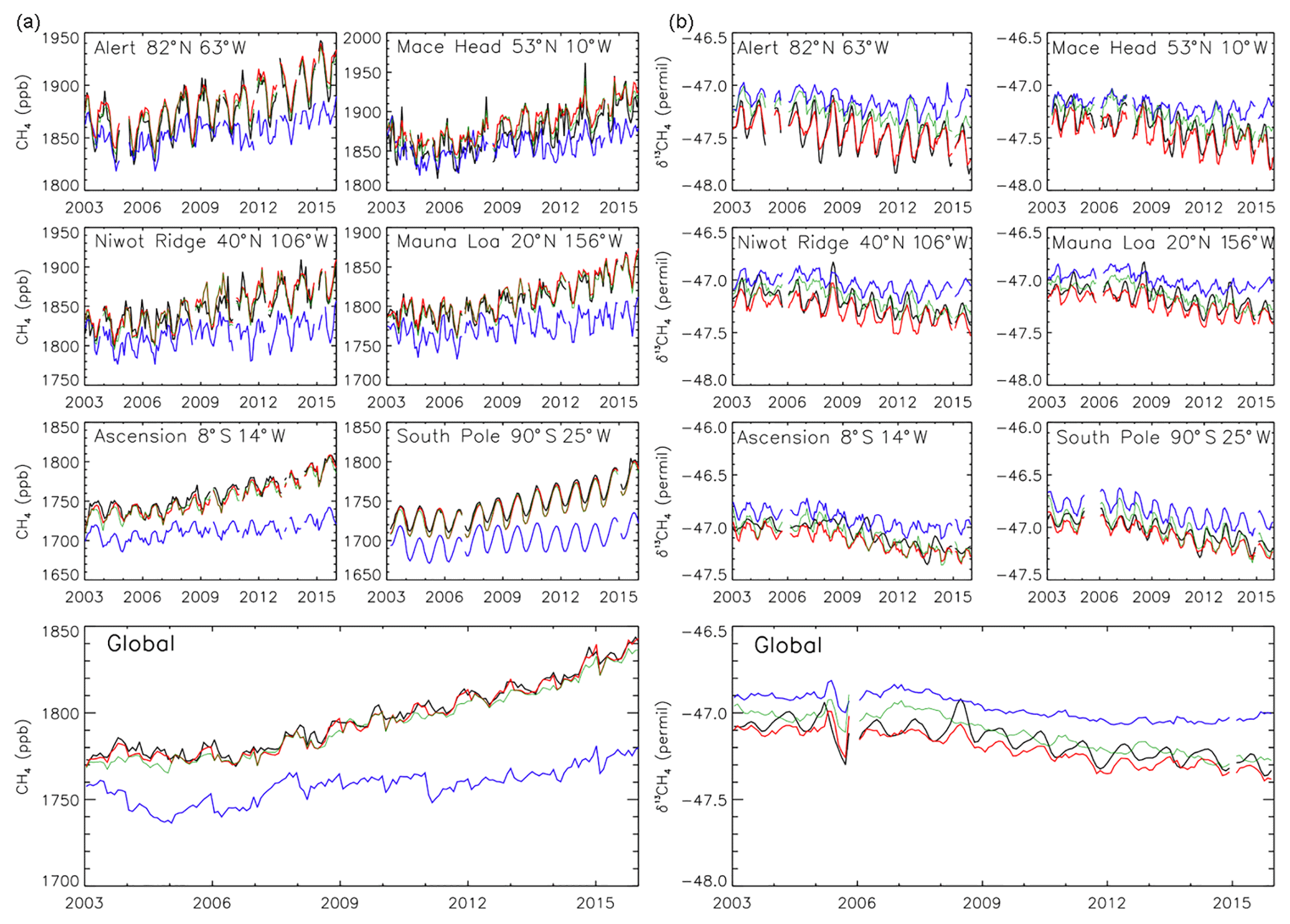
Figure 1(a) Observed surface CH4 (ppb, black line) from 2003 to 2015 at six selected NOAA sites and global mean. Also shown are results from TOMCAT simulations using prior emissions estimates (blue line), posterior estimates based on a CH4 synthesis inversion (INV-CH4, green line), and posterior estimates based on a combined CH4 and δ13CH4 synthesis inversion (INV-FULL, red line). (b) Same as (a) but for observed and modelled δ13CH4. Global averages are based on site interpolations onto 180 1∘ latitude bins, which are weighted by surface area.

Figure 2Monthly mean XCH4 volume mixing ratio (ppb) from GOSAT between April 2009 and December 2015 (black line) for five emissions regions. Also shown are results from TOMCAT simulations with prior (blue) and posterior (green) emissions estimates, both with GOSAT averaging kernels applied. Correlation coefficients, RMSE, and growth rates of the model simulations and GOSAT in each region are shown in the panels.
Inversion results constrained by CH4 (INV-CH4), and not δ13CH4, also accurately reproduce assimilated CH4 observations (R=0.93). INV-CH4 also shows some improved agreement with δ13CH4 observations relative to the prior (R=0.60), although values are overestimated in earlier years (2003–2008) (Fig. 1b).
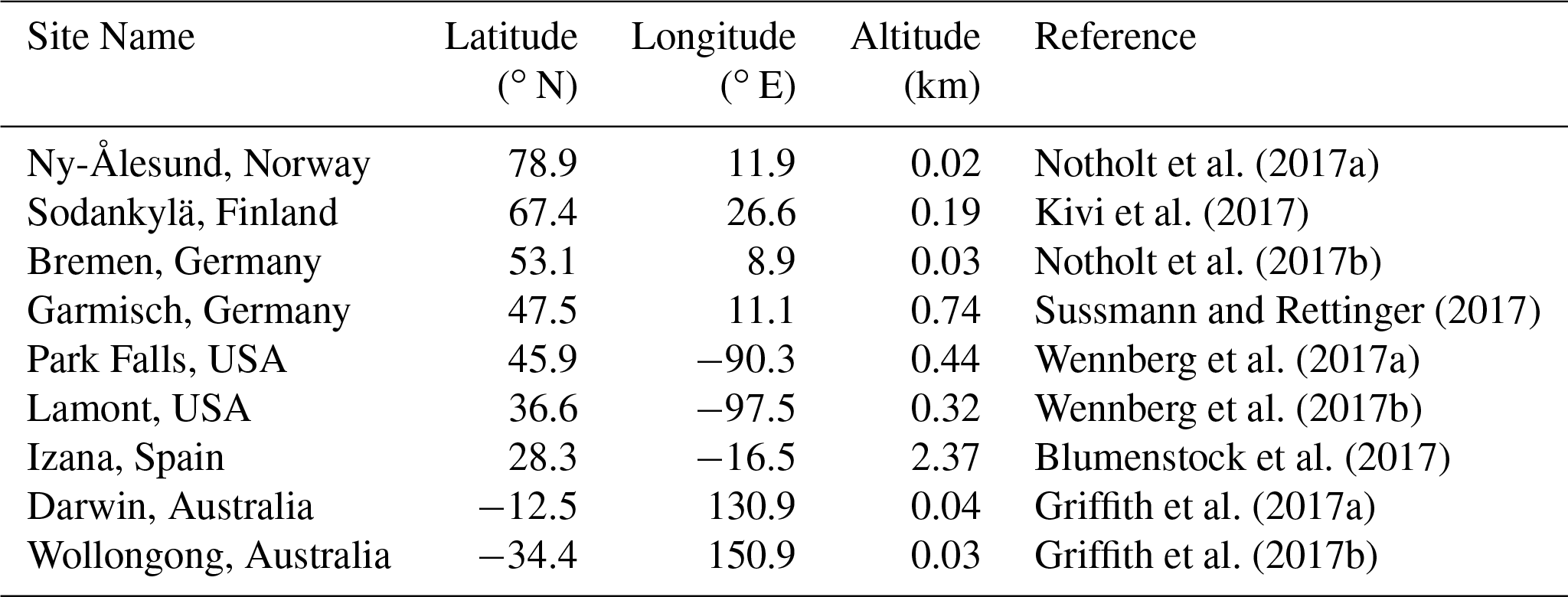
Table 3TCCON sites (Wunch et al., 2011) used for evaluation of the TOMCAT simulations.
Validation of the model inversion using the independent, non-assimilated GOSAT data shows improved seasonal and interannual representation of XCH4 (Fig. 2). The RMSE is reduced in all five regions with values ranging from 48.6 to 64.6 ppb in the prior to 8.3 to 16.5 ppb in the posterior, with values typically originating from a negative bias in the model. The correlation is increased in the inversion with R values ranging from 0.60 to 0.92 in the prior to 0.94 to 0.96 in the posterior. The trend is also better captured in the posterior in all five regions, although it is still underestimated in all regions, and more so in EA (−1.3 ppb yr−1) and AO (−1.1 ppb yr−1). Both the prior and posterior biases are larger in the Southern Hemisphere, possibly as a result of slow inter-hemispheric transport within the model, previously noted in Patra et al. (2011). Also contributing to this offset is an underestimation of Southern Hemisphere simulated atmospheric CH4 growth rates in the prior model simulation (Fig. 3).
We performed further validation using measurements from nine non-assimilated TCCON sites with data available from at least 2009 (see Table 3). The results show improved model–data correlation at all nine sites, with an increase in the all-site mean R value from 0.69 in the prior to 0.87 in the posterior (Fig. 4). The RMSE is reduced at sites; with an all-site mean decrease from 55.9 ppb in the prior to 18.8 ppb in the posterior, further reductions would be expected if column observations were used in the inversion. Overall the inversions are found to improve model–data agreement when validated against the independent measurements from both GOSAT and TCCON. The resulting Southern Hemisphere offset in the posterior relative to GOSAT and TCCON suggests the posterior estimates represent a reasonable but not conclusive scenario for source–sink attribution. As only surface sites are assimilated, some inaccuracy in the representation of the total column is not surprising.
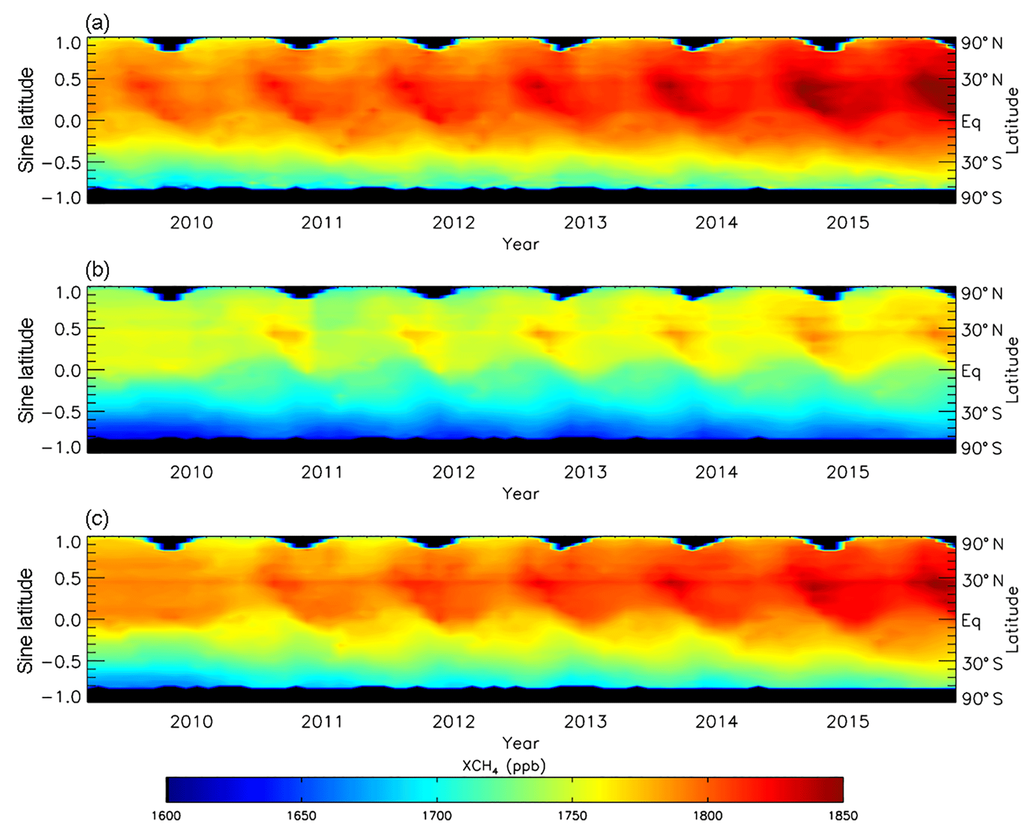
Figure 3(a) Zonally averaged monthly mean XCH4 volume mixing ratio (ppb) from GOSAT between April 2009 and December 2015 plotted against the sine of latitude, for which black denotes missing values. (b, c) Same as (a) but for TOMCAT simulations with prior and posterior emissions estimates, respectively. GOSAT averaging kernels are applied to model simulations.
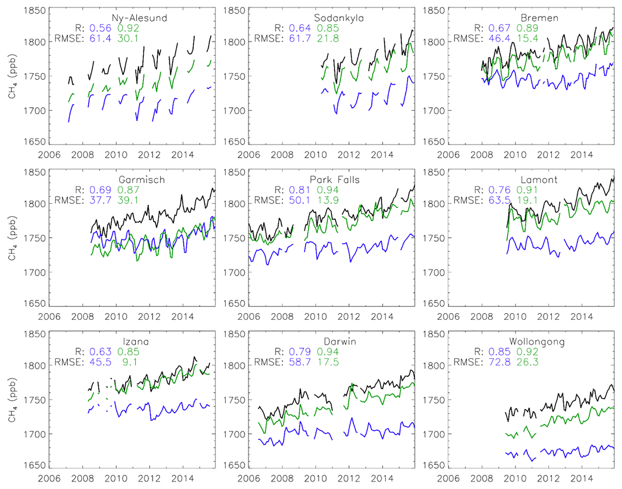
Figure 4Observed monthly mean XCH4 volume mixing ratio (ppb) (black line) at nine TCCON sites. Also shown are results from TOMCAT simulations with prior (blue) and posterior (green) emissions estimates, both with TCCON averaging kernels applied. Correlation coefficients and RMSE of the model simulations compared with TCCON are shown for each site.
Two surface sites were omitted from the inversion and retained for independent validation, HAGCOC and Cape Grim. Cape Grim is a baseline station, ideal for comparing the background signal (Fig. 5). Results at Cape Grim show improved model performance for both CH4 and δ13CH4, with respective RMSE decreases from 52.0 ppb and 0.2 ‰ in the prior to 12.3 ppb and 0.1 ‰ in the posterior and R value increases from 0.70 and 0.74 in the prior to 0.95 and 0.76 in the posterior. HAGCOC measurements are taken at high altitude (4464 m), which potentially provides insight into the vertical profile of measured species. As with Cape Grim, HAGCOC shows posterior improvements in both CH4 and δ13CH4, with respective RMSE decreases from 70.5 ppb and 0.2 ‰ in the prior to 27.1 ppb and 0.08 ‰ in the posterior and R value increases from 0.41 and 0.46 in the prior to 0.62 and 0.74 in the posterior.
3.2 Prior and posterior comparison
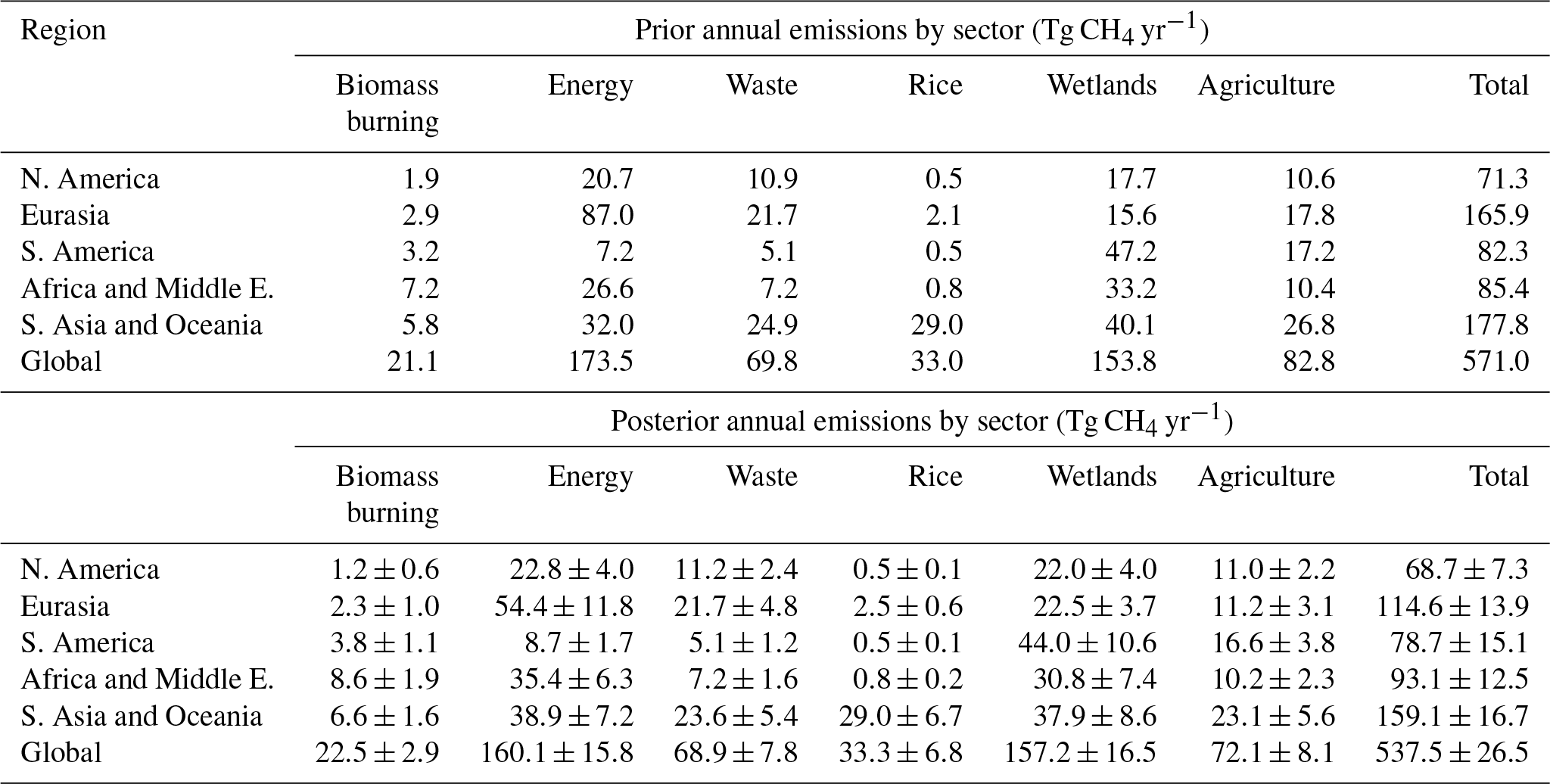
The synthesis inversions, INV-FULL and INV-CH4, provide posterior regional changes in sources and global changes in OH (Fig. 6). Relative to the prior, INV-FULL and INV-CH4 show an average OH decrease of 5 % and 4 %, respectively (Table 1). Results from INV-FULL show that globally agricultural (−13 %), energy (−8 %), and biomass burning (+7 %) emissions undergo the largest relative average 2003–2015 posterior change compared to the prior (Table 1). Relative changes in rice, waste, and wetlands are smaller (<3 %). The posterior emissions errors are between 5 % and 13 % compared with the 50 % prior error. Regionally (Fig. 7), 2003–2015 average posterior energy sector emissions are increased, relative to the prior, by 9 %–33 % in four regions (NA, SA, AM, and AO), which is offset by a 37 % decrease in EA. Notable posterior agricultural emissions decreases occur in EA (−36 %) and AO (−14 %). Wetland emissions are increased beyond the posterior error range in NA (+24 %) and EA (+44 %) and decreased within the error range in SA (−7 %), AM (−7 %), and AO (−6 %). In all regions posterior emissions estimates for biomass burning, waste, and rice are within, or close to, the error range compared with prior estimates (Table 4).
Table 4Regional CH4 emissions based on prior (top) and synthesis inversion estimates (bottom) between 2003 and 2015. Note the total global emissions, but not the total regional emissions, include the supplementary emissions (geological, hydrates, oceans, and termites). Uncertainties are also shown for posterior emissions; all prior emissions have a 50 % uncertainty.
Globally, for the 2003–2015 period, derived posterior and prior emissions estimates had average growth rates of 4.1±0.6 Tg yr−2 and 4.0±0.2 Tg yr−2, respectively. When considering only the renewed growth (2007–2015) the posterior growth rate of 5.7±0.8 Tg yr−2 becomes noticeably larger than the prior (3.7±0.4 Tg yr−2).
The seasonal range of the prior global wetland emissions (5.7 Tg month−1) is underestimated compared to the posterior (13.8 Tg month−1). The seasonal cycle in biomass burning emissions is largely unchanged between the prior and posterior. The seasonal amplitude in rice emissions also remains largely unchanged, although the seasonal peak occurs in August in the prior and July in the posterior (Fig. 6).
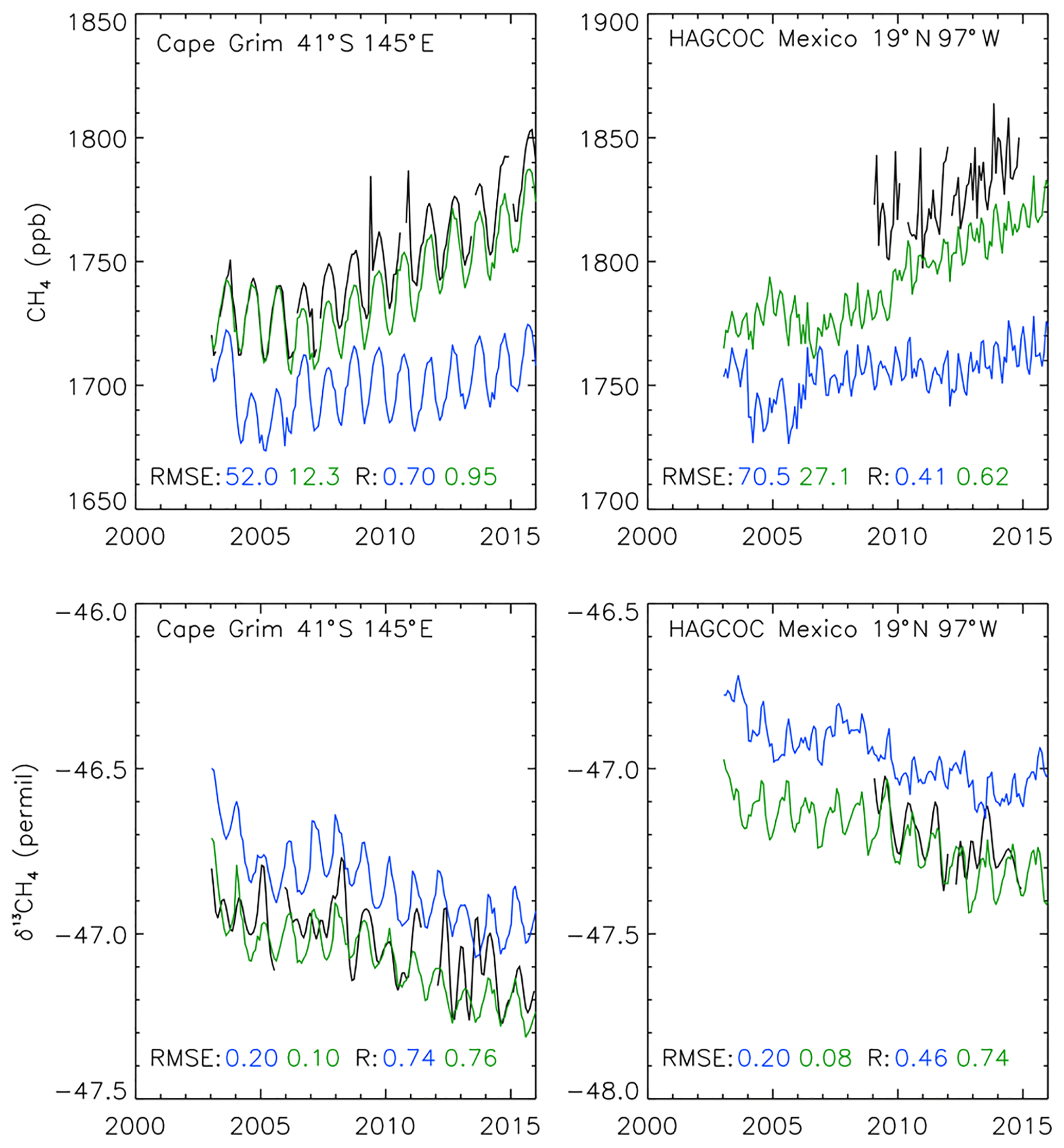
Figure 5Observed surface CH4 (top) and δ13CH4 (bottom) from 2003 to 2015 at two independent NOAA sites (black line). Also shown are results from TOMCAT simulations using prior emissions estimates (blue line), and posterior estimates based on a combined CH4 and δ13CH4 synthesis inversion (INV-FULL, green line). RMSE and correlation coefficients of the model simulations compared with observations are shown for each site.
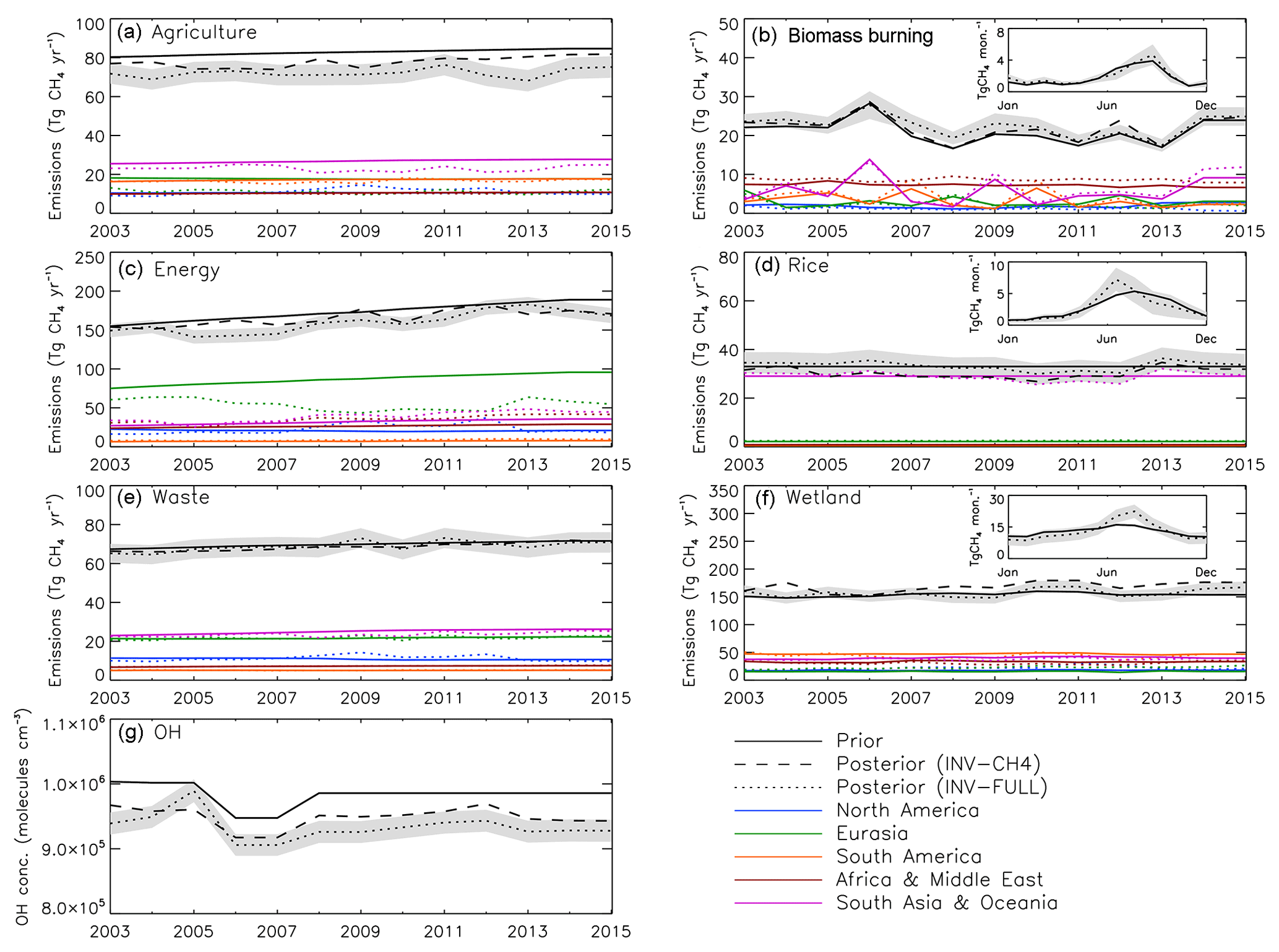
Figure 6(a–f) Annual CH4 emissions (Tg CH4 yr−1) from different sectors for global prior (black solid line), INV-CH4 (black dashed line), and INV-FULL posterior (black dotted line) estimates. Regional estimates are also displayed for North America (blue), Eurasia (green), South America (orange), Africa and the Middle East (red), and South Asia and Oceania (purple). (g) Prior and posterior global OH estimates for the same period. Shaded region denotes posterior error A for INV-FULL (see Eq. 5 in text).
3.3 Time trends in sources and sinks
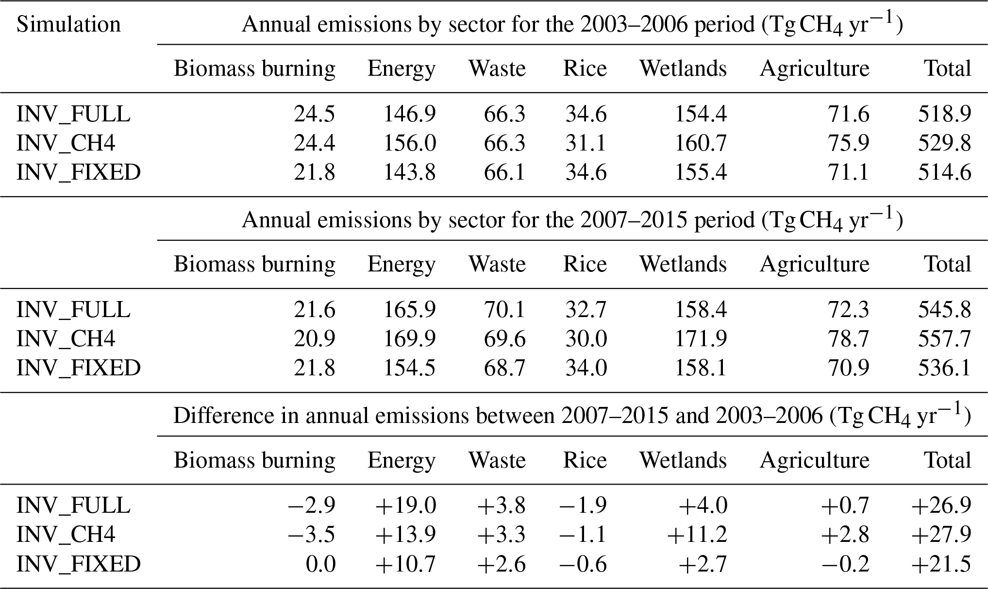
Average energy, waste, and wetland emissions are increased after 2007 by 12.9±2.7 % (19.0 Tg yr−1), 5.7±1.6 % (3.8 Tg yr−1), and 2.6±1.8 % (4.0 Tg yr−1), respectively, relative to their 2003–2006 posterior values (Table 6). Regionally, the shift in post-2007 energy sector emissions mainly occurs in AM (+8.4 Tg yr−1) and AO (+11.1 Tg yr−1). Four out of five of the regions show a positive post-2007 shift in waste emissions of 0.4–1.4 Tg yr−1, SA is the only region with a slight decrease (−0.03 Tg yr−1). The small increase in wetland emissions since 2007 derived from the inversion, mainly from EA (3.4 Tg yr−1), agrees well with bottom-up estimates for wetland emissions trends, for example the 3 % increase found by McNorton et al. (2016a). The posterior shows a negative shift in posterior biomass burning emissions of 11.8±6.4 % (−2.9 Tg yr−1) for the 2007–2015 period relative to 2003–2006, which is in partial agreement with the 3.7 Tg CH4 yr−1 decrease derived by Worden et al. (2017) for the 2008–2014 period relative to 2001–2007. This shift occurs in all five regions, with the largest decrease in AO (−1.2 Tg yr−1). Overall the derived increase in energy sector, waste, and wetland emissions coupled with the decrease in biomass burning emissions agree well with a recent budget review (Saunois et al., 2017).
The post-2007 posterior emissions growth occurs mainly in the energy (3.4±1.0 Tg yr−2) and wetland (1.4±1.0 Tg yr−2) sectors. For the entire period most of the posterior energy sector growth occurred in AM (1.2 Tg yr−2) and AO (1.5 Tg yr−2), with a smaller proportion from NA (0.6 Tg yr−2) and SA (0.2 Tg yr−2) (Fig. 7 and Table 5). The recent EDGAR v4.3.2 inventory (Janssens-Maenhout et al., 2017) for energy sector emissions shows AM and AO growth of 1.0 and 2.4 Tg yr−2, respectively, for 2003–2012. This is smaller than the 2.2 and 3.1 Tg yr−2 shown by our inversion for the same period. The majority of prior AM energy sector emissions originate from energy for buildings in Nigeria and eastern Africa, fuel exploitation from the Middle East, the Niger Delta, and South Africa, and pipelines in western Africa, Algeria, and the Middle East. The regional aggregation of fluxes in our inversion system prevents subregional attribution, as a result we are unable to diagnose more specific posterior spatial patterns, but our results suggest, on a regional scale, emissions are underestimated in both magnitude and growth rate in the prior. For the AO energy sector, the majority of prior emissions, and therefore the posterior increases, originate from energy for buildings in India, China, and South East Asia; fuel exploitation in eastern China, Japan, India, South East Asia and eastern Australia; refineries in northern India, eastern China, Japan, and Indonesia; and pipelines in India, eastern China, eastern Australia, and New Zealand. The growth in emissions in EA in EDGAR v4.3.2 for 2003–2012 (1.4 Tg yr−2) is not seen in our inversion for the same region and period (−2.2 Tg yr−2).
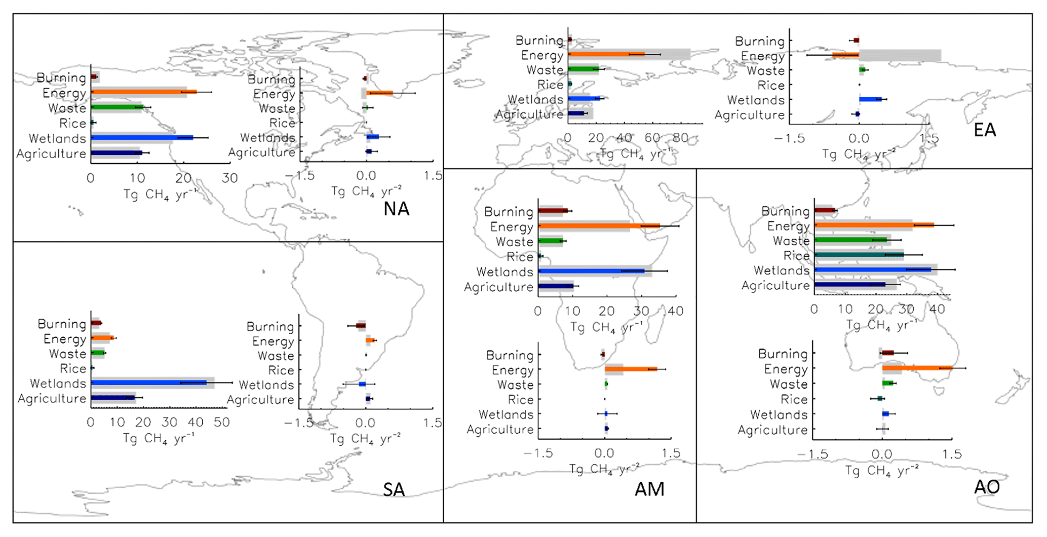
Figure 7Map showing regional annual mean CH4 emissions (Tg CH4 yr−1) and yearly change in emissions (Tg CH4 yr−2) calculated as a linear regression between 2003 and 2015 for INV-FULL (thin coloured bars) and prior (thick grey bars) estimates. Error bars represent 1 standard deviation of the mean posterior emissions and posterior regression errors. Note that the black borders indicate the five regions used for the flux partitioning.
Table 5Regional CH4 emissions growth trends based on synthesis inversion estimates between 2003 and 2015.
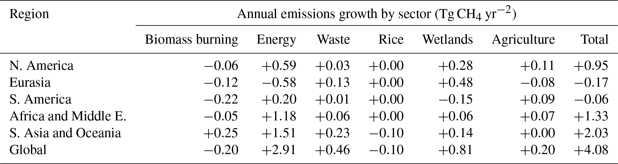
Table 6Posterior annual CH4 emissions for the period of near-zero atmospheric growth (2003–2006) and the renewed growth (2007–2015) based on three different inversion simulations. Note the total emissions include the supplementary emissions (geological, hydrates, oceans, and termites).
During the 2008–2012 period NA energy sector emissions were found to be 11.4 Tg yr−1 (+66 %) higher than the 2003–2015 (excluding 2008–2012) average, resulting in uncertainty in the NA growth rate (Fig. 6). These findings are also present in INV-CH4, which shows an 11.8 Tg yr−1 increase over the same period. This period of anomalously high emissions is not present in the prior and therefore is due to the assimilated observations. These high emissions may be associated with oil or natural gas extraction (Helmig et al., 2016). During periods of high NA energy sector emissions, the EA energy sector emissions are reduced and vice versa, suggesting a possible dipole caused by the inversion. This suggests increased uncertainty in the derived EA and NA energy sector emissions, possibly due to a paucity of observations over these regions.
Posterior wetland emissions estimates show a growth of 0.8 Tg yr−2 for the 2003–2015 period, which increases to 1.4 Tg yr−2 for the 2007–2015 period. The majority of this growth occurs in EA (+0.5 Tg yr−2). The four remaining emissions sectors all have a global annual change of less than ±0.5 Tg yr−2.
For the posterior time series, OH concentrations in INV-FULL and INV-CH4 are relatively constant throughout the period of 2007–2015 (Fig. 6), but relative to their 2003–2006 concentrations these values are smaller by 1.8±0.4 % and 0.3±0.5 %, respectively. The larger drop after 2007 in INV-FULL OH concentration, relative to INV-CH4, highlights the importance of including δ13CH4 in the inversion. A decrease in OH as a contributor to the renewed growth agrees well with previous simple global box models (Rigby et al., 2017; Turner et al., 2017). The OH shift found here is smaller in magnitude than the −8 % shift between 2004 and 2014 derived by Rigby et al. (2017) and the −7 % shift between 2003 and 2016 derived by Turner et al. (2017). The posterior OH error is reduced from the prior estimate of 2 % to 1.8 %, which, although a reduction, is similar to the modelled post-2007 OH decrease. The decrease in OH contributes to a decrease in δ13CH4 and an increase in global CH4. Section 3.5 details analysis of OH sensitivity.
3.4 Source and sink attribution
Analysis performed on our inversion results using the box model approach described by McNorton et al. (2016b) suggests that ∼30 % of the sustained CH4 growth after 2007 can be explained by decreased OH, while ∼60 % and ∼10 % is attributed to an increased energy sector and wetland emissions (Table 5). The shift in emissions between 2003–2006 and 2007–2015 is broadly consistent for each sector for three different inversions, INV_FULL, INV_CH4, and INV_FIXED (fixed annual emissions; see below) (Table 6). We investigated source and sink contribution to the negative δ13CH4 trend using simple one box model analysis, outlined in the appendix of McNorton et al. (2016b), and posterior estimates from INV-FULL. Results show that post-2007 changes in energy sector (+0.15 ‰), biomass burning (−0.08 ‰), wetland (−0.05 ‰), waste sector (−0.03 ‰), and agricultural (−0.01 ‰) emissions, as well as OH (−0.12 ‰), contributed to the observed trend.
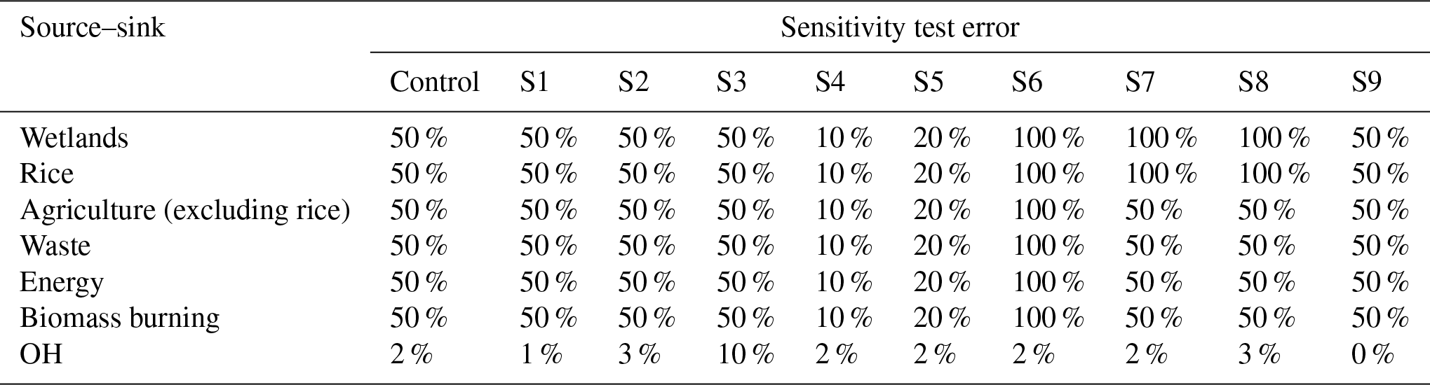
Table 7Suite of inversion sensitivity experiments with varying errors on source and sink estimates.
3.5 Sensitivity tests
To test the robustness of the inversion to changes in prior error estimates we performed nine perturbation experiments (S1–S9). Monthly source errors were perturbed between 10 % and 100 % and yearly OH errors from 0 % to 10 % (Fig. 8 and Table 7). For small error perturbations, the inversion results do not change much relative to INV-FULL (Fig. 8 and Table 8). However, when the emissions errors are reduced from 50 % to 10 % (S4) the posterior energy emissions estimates deviate from the control (INV-FULL) inversion, with a mean bias of 60.5 Tg yr−1. We consider these large ranges in posterior estimates to be an unrealistic representation of interannual variability in energy sector emissions (Fig. 8), which suggests the model fails to provide reasonable posterior estimates when the prior emissions error is set too low. For most cases of increased emissions errors the OH change is similar to the control. However, for 100 % emissions errors (S6) the agricultural emissions are further reduced, from 82.8 Tg yr−1 in the prior and 72.1 Tg yr−1 in INV-FULL to 64.1 Tg yr−1. In this case OH is only reduced by 0.5 % after 2007, relative to 2003–2006, compared to 1.8 % in INV-FULL. This results in a smaller OH contribution to the post-2007 CH4 growth.

Figure 8(a–f) Annual mean CH4 emissions (Tg CH4 yr−1) from different sectors for global prior (black solid line) and INV-FULL (black dotted line) estimates. (g) Same as (a–f) but for global mean OH (molecules cm−3). Additional lines in each panel show sensitivity inversions with different emissions and OH uncertainties (coloured lines) and an inversion assuming no change in OH (black dashed line).
Table 8Posterior annual CH4 emissions for the period of near-zero atmospheric growth (2003–2006) and the renewed growth (2007–2015) based on a suite of inversion sensitivity experiments with varying errors on source and sink estimates. Note the total emissions include the supplementary emissions (geological, hydrates, oceans, and termites).
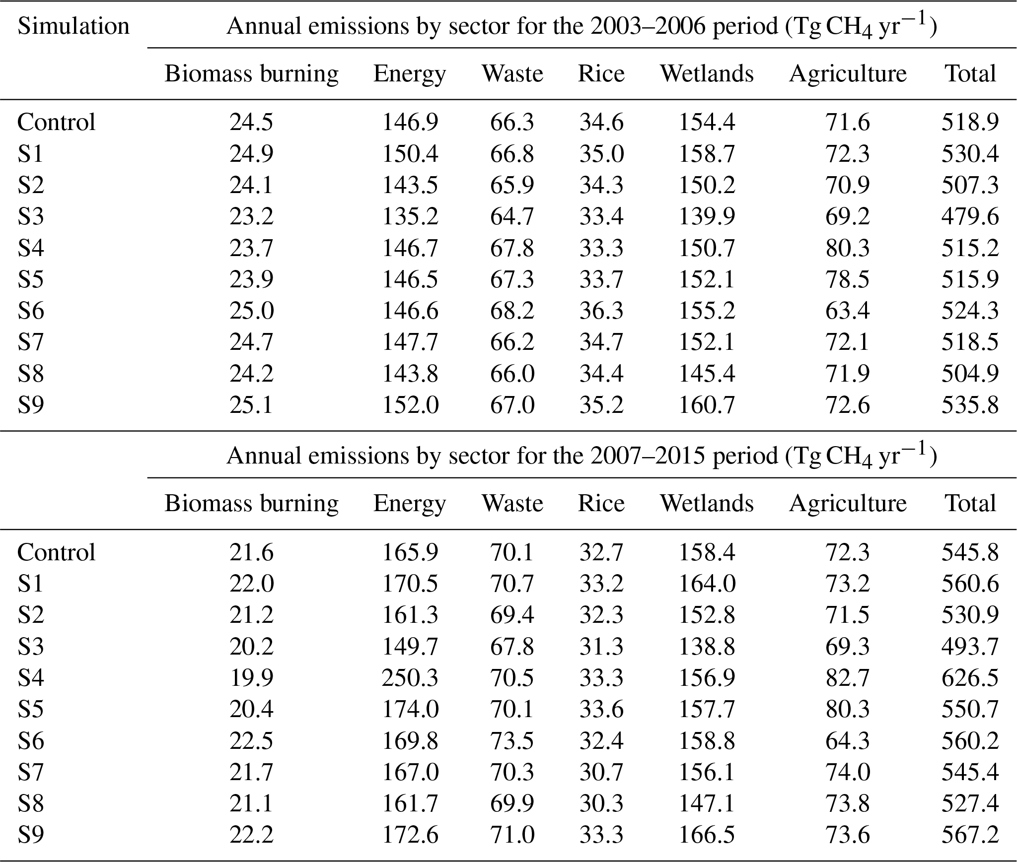
For large or small OH errors (S3: 10 %; S1: 1 %) the posterior OH is decreased by 18 % or 2 %, respectively, compared to the prior OH. Assuming no change in OH (S9) post-2007 shifts in biomass burning, energy sector, and wetland emissions relative to 2003–2006 are required to fit observations in the inversion. In this scenario biomass burning emissions decrease globally by % (−2.9 Tg yr−1), and in AO by % (−1.2 Tg yr−1). Energy sector emissions increase globally by 13.6±2.7 % (+20.6 Tg yr−1), in NA by 42.9±12.9 % (+7.7 Tg yr−1) and in AO by 36.7±5.1 % (+12 Tg yr−1). Wetland emissions increase globally by 3.6±1.8 % (+5.8 Tg yr−1). The sign and spatial distribution of these changes are similar to those seen in INV-FULL, although the magnitude in post-2007 changes is typically increased in S9 (see Sect. 3.2), which is expected as the necessary increased growth rate is allocated more to emissions changes when OH is assumed constant.
The sensitivity analyses highlight that the prior uncertainty can have a noticeable influence on the posterior estimates. In particular, the posterior OH is found to be sensitive to the prior error estimate, highlighting the importance of prior knowledge for future studies. This limits the accuracy of the magnitude of the posterior estimates. However, the spatial, temporal, and sector-specific relative post-2007 changes, compared to 2003–2006, remain broadly consistent among experiments. This shows a limitation in the comparison between prior and posterior sources–sinks but does not discount the importance of the results for trend detection between 2003 and 2015.
We performed a synthesis inversion with no prior trend in emissions or OH (INV-FIXED), using fixed 2003 emissions, to investigate the sensitivity of the inversion to prescribed prior trend information (Fig. 9). The results show an annual average CH4 emissions growth of 2.8±0.6 Tg yr−2, the majority of which comes from the energy sector (1.8±0.6 Tg yr−2) and wetlands (0.7±0.5 Tg yr−2). On a global scale the sector attribution agrees well with INV-FULL but with a smaller magnitude in emissions trends. The reduced growth in INV-FIXED is offset by a higher negative trend in OH concentration (−0.23 % yr−1), relative to INV_FULL (−0.14 % yr−1).
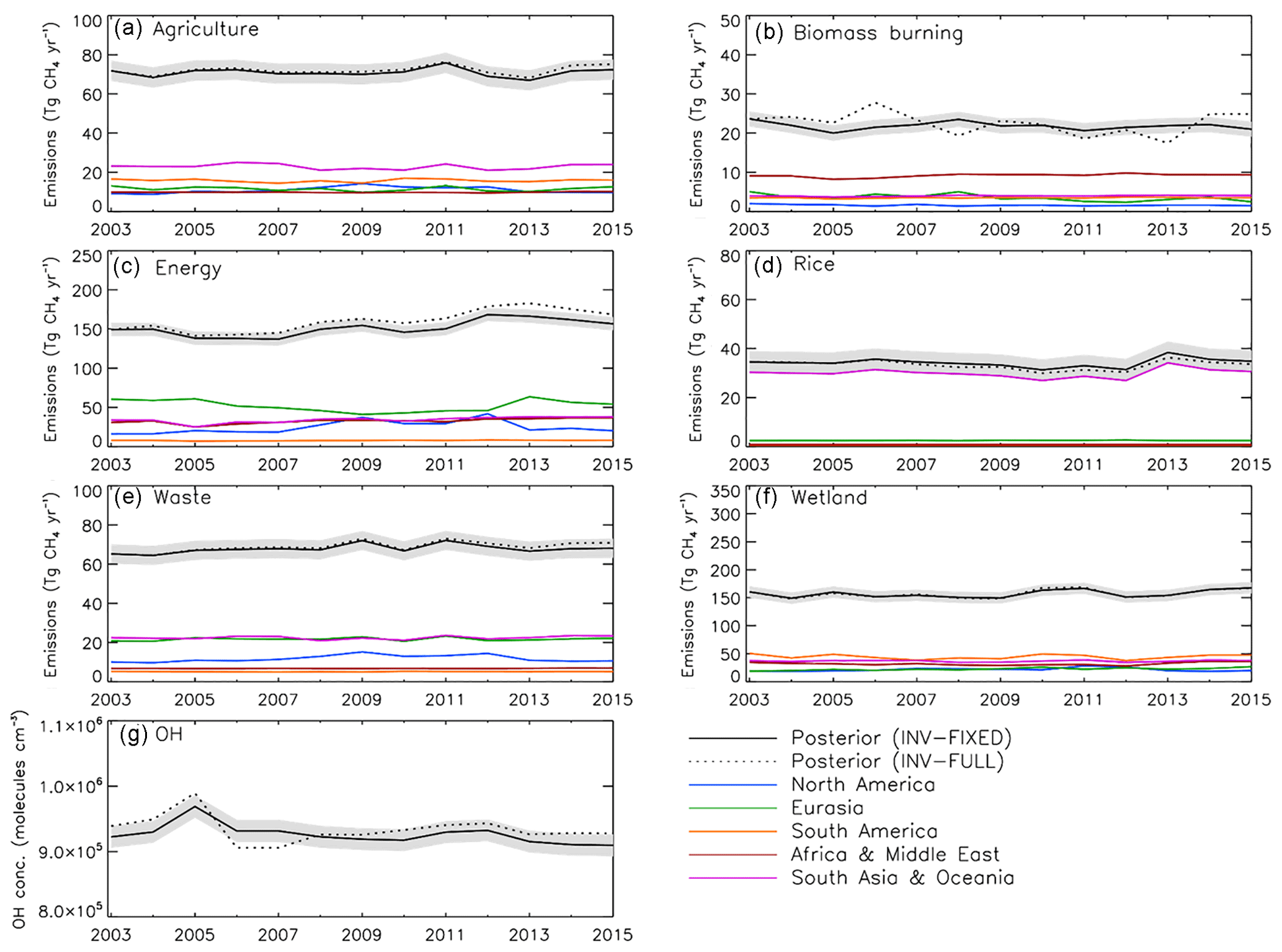
Figure 9(a–f) Annual CH4 emissions (Tg CH4 yr−1) from different sectors for INV-FIXED (black solid line) and INV-FULL posterior (black dotted line) estimates. Regional estimates are also displayed for North America (blue), Eurasia (green), South America (orange), Africa and the Middle East (red), and South Asia and Oceania (purple). (g) INV-FIXED (black solid line) and INV-FULL (black dotted line) posterior global OH estimates (molecules cm−3) for the same period. Shaded region denotes posterior error A (see Eq. 5 in text).
In absolute terms OH concentrations are 0.8 % lower in INV-FIXED compared to INV-FULL, which acts to offset the lower emissions. OH concentrations for INV-FIXED are 1.8 % lower for the 2007–2015 period, relative to the 2003–2006 period, matching the relative change from INV-FULL. Regionally, the largest trends are observed over NA (1.2±0.9 Tg yr−2), AM (0.9±0.3 Tg yr−2), and AO (0.7±0.4 Tg yr−2), with over half of the growth in each of those regions originating from the energy sector. Overall INV-FIXED shows good spatial agreement with INV-FULL when considering sector attribution but the magnitude of emissions increases is slightly smaller.
Tropospheric Cl only accounts for a small fraction of the total CH4 sink (∼5 % or less) (Kirschke et al., 2013; Hossaini et al., 2016) but, as the kinetic fractionation of Cl reacting with CH4 is more than an order of magnitude greater than that of OH, it is plausible that changes in Cl could contribute to the post-2007 trend in δ13CH4. In results from an experiment that inverts for CL, INV-CL (Fig. 10) and the sensitivity set-up with fixed OH show similar posterior fluxes. This suggests that Cl trends and their effect on δ13CH4 are unlikely to be an important contributor to the post-2007 CH4 trends, although it is important to note that whilst variability was applied to prior emissions and the OH field, for some years, no variability is applied to the prior Cl field.

Figure 10(a–f) Annual CH4 emissions (Tg CH4 yr−1) from different sectors for global prior (black solid line) and INV-CL (black dotted line) estimates. Regional estimates are also displayed for North America (blue), Eurasia (green), South America (orange), Africa and the Middle East (red), and South Asia and Oceania (purple). (g) Prior and posterior global tropospheric Cl estimates for the same period. Shaded region denotes posterior error A (see Eq. 5 in text).
3.6 Posterior error
The robustness of the experimental set-up is further investigated using the posterior error covariance matrix calculated using Eq. (5). By splitting the inversion into 12-month intervals, emissions later in the year are constrained by fewer observations, possibly only by observations close to the source. The influence of this was investigated and the posterior error was found to be on average 12 % higher for December emissions relative to the January emissions, which was broadly consistent among regions and sectors.
Relatively small time-independent off-diagonal error correlations are found among different regions and sectors (Fig. 11). The posterior covariances produced using Eq. (5) have been normalised using the corresponding posterior standard deviations to provide posterior correlation values. The largest negative correlation is between EA and NA energy sector emissions, which suggest an artificial trade-off of our results with the increasing NA emissions over 2008–2012 being offset by a decrease in EA emissions over the same period. Overall the results are well constrained by the inversion. Typically, the temporal error correlation is also found to be relatively small, with the exception being the energy sector emissions. Both positive and negative off-diagonal error correlations are found in posterior energy estimates at a monthly resolution, possibly relating to the prior temporal correlation applied; as a result we typically report annual values.
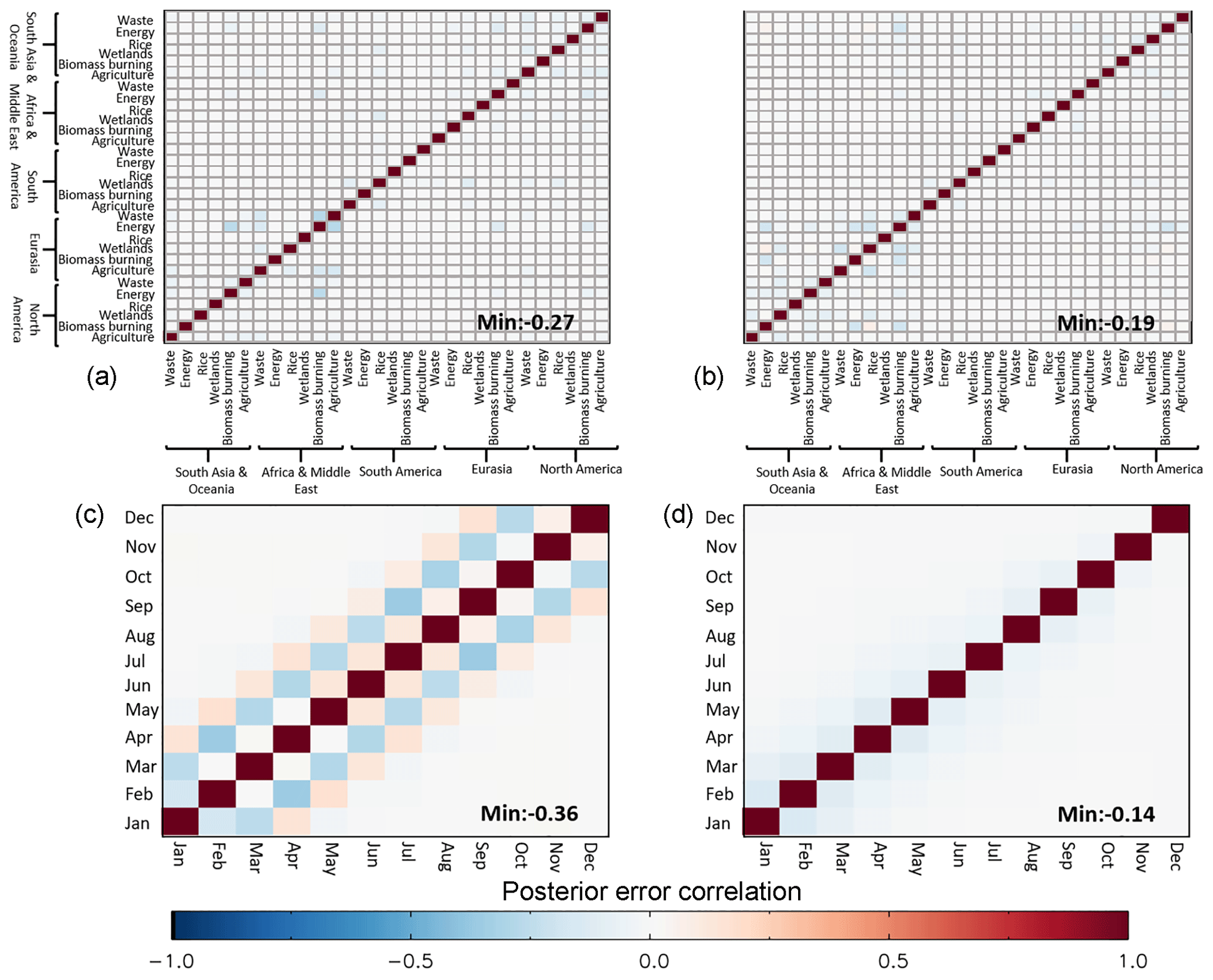
Figure 11Posterior error correlation matrix for all regions and sectors for January (a) and July (b) 2015. Posterior error correlation matrix for 12 months in 2015 for the Eurasian energy sector (c) and South American wetlands (d). The plots show a subset of the total posterior error correlation matrix as an example. Values are calculated by normalising the posterior covariances using the corresponding posterior standard deviations.
We have performed a synthesis inversion using a 3-D CTM to investigate the post-2007 renewed growth in atmospheric CH4 and decline in δ13CH4. This work adds to the results from other studies, which were based on a box model approach for source and sink attribution based on CH4 and δ13CH4 observations (e.g. Rigby et al., 2017). By using a 3-D CTM we have been able to provide detailed monthly regional attribution of six different emissions sectors and global OH changes, evaluating both the trends over the full 2003–2015 period and shifts that occurred around 2007. We have also been able to validate these results using independent surface sites and recent XCH4 data available from GOSAT and TCCON. The sensitivity of the inversion has been tested for different prior assumptions and uncertainties.
A CH4-only inversion under-constrains the solution with respect to 13CH4 observations, resulting in reduced correlation with δ13CH4 observations (R=0.60). The agreement of the simulations with observations improved when additional 13CH4 observations were used to constrain CH4 fluxes, with the correlation increasing to R=0.87. The prior model based on published emissions does not capture the CH4 and δ13CH4 trend either at the assimilated surface site observations or in the non-assimilated GOSAT and TCCON data. In contrast, our derived posterior emissions inventories capture both the renewed growth in CH4 and the reduction in δ13CH4 observed from the assimilated NOAA surface sites from 2007 to 2015 and compare well with independent surface CH4 and δ13CH4 observations as well as with GOSAT and TCCON-derived XCH4. The independent validation suggests that, although the CH4 growth rate is better represented in the posterior, it is still underestimated. The posterior model agreement with assimilated surface data and slight bias with validation column data (TCCON and GOSAT) highlight a potential a posteriori model error in total column CH4 concentrations; however, this bias is small. The magnitude of the contribution of model transport error to this underestimation is unknown. Both prior and posterior simulations underestimate Southern Hemisphere CH4 concentrations, highlighting possible issues with interhemispheric transport within the model. The lack of independent data around the end of the CH4 “hiatus” means it is difficult to evaluate model performance over this period (2007).
Our inversion results suggest that the 2007–2015 growth in CH4 can be best explained by a 1.8±0.4 % reduction in mean OH, a 12.9±2.7 % increase in energy sector emissions, mainly from AM and AO, and a 2.6±1.8 % increase in wetland emissions, mainly from EA. The expected increase in atmospheric δ13CH4 caused by increased energy sector emissions (+0.15 ‰) is offset mainly by the decrease in OH (−0.12 ‰), small decrease in biomass burning emissions (−0.08 ‰), and small increase in wetland emissions (−0.05 ‰).
When δ13CH4 is not assimilated the trend in posterior emissions is slightly increased after 2007 and the OH decrease is smaller (−0.3 %). By including the δ13CH4 observations, a larger post-2007 OH decrease is required (−1.8 %), highlighting the importance of including δ13CH4 within the inversion.
An alternative scenario, in which OH is assumed constant after 2007, requires a % decrease in biomass burning emissions and 13.6±2.7 % and 3.6±1.8 % increases in energy sector and wetland emissions. These results agree with previous studies, which also assumed constant OH (Nisbet et al., 2016; Schaefer et al., 2016; Worden et al., 2017). Whilst a reduction in OH is found to be, in part, the most likely explanation for the renewed CH4 growth, this alternative scenario with no change in OH provides an alternative explanation for the cause of the post-2007 CH4 growth.
The inversion results suggest Eurasian energy sector emissions are typically overestimated by inventories and previous top-down studies, such as the Global Carbon Budget (Saunois et al., 2016). The reduced EA emissions are found to be offset by an underestimate in all other regions. We find prior annual estimates of biomass burning, waste, and rice to be relatively accurate, whilst agricultural estimates are overestimated. Small changes occur in the seasonal cycle of rice emissions and the seasonal range is underestimated in wetland emissions.
Our inversion is found to be robust when small changes are made to uncertainty errors; however, large uncertainty remains around the accuracy of prior emissions. Assuming no prior trend in emissions reduces the required growth rate in both wetland and energy sector emissions, although they remain the main source contribution to the renewed growth after 2007. The reduction in the emissions trend is offset by an increased negative trend in OH concentration. Overall the magnitude of the trends inferred varies among experiments but there is consistent agreement that both OH decrease and wetland and energy sector emissions increase contributed to the post-2007 growth.
Our inversion results represent plausible scenarios for variations in CH4 sources and sinks, though several caveats exist. The uncertainties in the sources and sinks are somewhat subjective and we have not considered source signature and kinetic fractionation uncertainty. We have assumed that all uncertainties are independent of each other (excluding energy emissions). We have also not considered variation in other sinks (e.g. O(1D), soil). The synthesis inversions are performed over coarse spatial regions and only attribute emissions at the monthly scale; future studies should utilise increased observations to provide finer spatial and temporal resolution. The assumption that emissions within a region are correlated limits more specific spatial attribution of sources. Within a region it is likely that some posterior emissions are too high, offset by emissions being too low elsewhere within the domain. The choice of regional aggregation is likely to influence the synthesis inversion, which may result in aggregation errors causing biases in the posterior fluxes (Kaminski et al., 2001). Finally, an important question is whether tropospheric OH has varied in the way suggested by CH4 inversion studies. The processes causing variations in OH are complex and remain poorly quantified. Possible explanations include changes in tropospheric O3 and trends in tropospheric UV radiation related to global stratospheric O3 recovery. If the reduction in available OH due to increased reactive carbon gases is no longer being sufficiently offset by increased emissions of OH-forming nitrogen oxides, then OH concentrations might be in decline (Lelieveld et al., 2004). For example, Itahashi et al. (2014) showed a reduction in column NO2 growth associated with the economic downturn over East Asia between 2008 and 2009, which approximately coincides with the increased CH4 growth.
All model data used in this study are available through the University of Leeds FTP server. For access please contact Martyn P. Chipperfield (m.chipperfield@leeds.ac.uk).
JM, CW, MG, and MPC designed the model experiment. CW developed the synthesis inversion methodology. RJP and HB performed GOSAT retrievals for validation. WF, JM, CW, and MPC developed the modeling tools used for the experiment. JM and CW performed model simulations. RH developed the model chlorine field. JM, CW, MG, and MPC wrote the paper with contributions from all coauthors.
This work was supported by the NERC MOYA project (NE/N015657/1). Martyn P.
Chipperfield and Manuel Gloor acknowledge support from NERC grants GAUGE
(NE/K002244/1) and AMAZONICA (NE/F005806/1). Rob J. Parker was funded via an
ESA Living Planet Fellowship with additional funding from the UK National
Centre for Earth Observation and the ESA Greenhouse Gas Climate Change
Initiative (GHG-CCI). Hartmut Boesch was supported by ESA GHG-CCI. Chris
Wilson, Rob J. Parker, and Hartmut Boesch acknowledge funding support as part
of NERC's National Centre for Earth Observation, contract number PR140015.
The TOMCAT runs were performed on the Arc3 supercomputer at the University of
Leeds. We thank the Japanese Aerospace Exploration Agency, National Institute
for Environmental Studies, and the Ministry of Environment for the GOSAT data
and their continuous support as part of the Joint Research Agreement. The
GOSAT retrievals used the ALICE High Performance Computing Facility at the
University of Leicester. NOAA atmospheric CH4 and δ13CH4 values were obtained from the ESRL GMD Carbon Cycle Cooperative
Global Air Sampling Network (https://esrl.noaa.gov/, last access:
5 October 2017). TCCON atmospheric column CH4 values were obtained
from the TCCON data archive (https://tccondata.org/). The authors would
also like to thank Matt Rigby for advice with 13CH4 modelling.
Edited by: Patrick Jöckel
Reviewed by: two anonymous referees
Bergamaschi, P., Frankenberg, C., Meirink, J. F., Krol, M., Dentener, F., Wagner, T., Platt, U., Kaplan, J. O., Körner, S., Heimann, M., and Dlugokencky, E. J.: Satellite chartography of atmospheric methane from SCIAMACHY on board ENVISAT: 2. Evaluation based on inverse model simulations, J. Geophys. Res., 112, D02304, https://doi.org/10.1029/2006JD007268, 2007.
Blumenstock, T., Hase, F., Schneider, M., García, O. E., and Sepúlveda, E.: TCCON data from Izana, Tenerife, Spain, Release GGG2014R1, TCCON data archive, hosted by CaltechDATA, California Institute of Technology, Pasadena, CA, USA, https://doi.org/10.14291/tccon.ggg2014.izana01.R1, 2017.
Bousquet, P., Ciais, P., Miller, J. B., Dlugokencky, E. J., Hauglustaine, D. A., Prigent, C., Van der Werf, G. R., Peylin, P., Brunke, E. G., Carouge, C., and Langenfelds, R. L.: Contribution of anthropogenic and natural sources to atmospheric methane variability, Nature, 443, 439–443, https://doi.org/10.1038/nature05132, 2006.
Bousquet, P., Ringeval, B., Pison, I., Dlugokencky, E. J., Brunke, E.-G., Carouge, C., Chevallier, F., Fortems-Cheiney, A., Frankenberg, C., Hauglustaine, D. A., Krummel, P. B., Langenfelds, R. L., Ramonet, M., Schmidt, M., Steele, L. P., Szopa, S., Yver, C., Viovy, N., and Ciais, P.: Source attribution of the changes in atmospheric methane for 2006–2008, Atmos. Chem. Phys., 11, 3689–3700, https://doi.org/10.5194/acp-11-3689-2011, 2011.
Chipperfield, M.: New version of the TOMCAT/SLIMCAT off-line chemical transport model: Intercomparison of stratospheric tracer experiments, Q. J. Roy. Meteor. Soc., 132, 1179–1203, https://doi.org/10.1256/qj.05.51, 2006.
Dee, D. P., Uppala, S. M., Simmons, A. J., Berrisford, P., Poli, P., Kobayashi, S., Andrae, U., Balmaseda, M. A., Balsamo, G., Bauer, D. P., and Bechtold, P.: The ERA-Interim reanalysis: Configuration and performance of the data assimilation system, Q. J. Roy. Meteor. Soc., 137, 553–597, https://doi.org/10.1002/qj.828, 2011.
DeFries, R. S. and Townshend, J. R. G.: NDVI-derived land cover classification at a global scale, Int. J. Remote Sens., 15, 3567–3586, https://doi.org/10.1080/01431169408954345, 1994.
Dlugokencky, E. J., Lang, P. M., Crotwell, A. M., Mund, J. W., Crotwell, M. J., and Thoning, K. W.: Atmospheric Methane Dry Air Mole Fractions from the NOAA ESRL Carbon Cycle Cooperative Global Air Sampling Network, 1983–2016, Version: 2017-07-28, available at: ftp://aftp.cmdl.noaa.gov/data/trace_gases/ch4/flask/surface/, last access: 5 October 2017.
Feilberg, K. L., Griffith, D. W., Johnson, M. S., and Nielsen, C. J.: The 13C and D kinetic isotope effects in the reaction of CH4 with Cl, Int. J. Chem. Kinet., 37, 110–118, https://doi.org/10.1002/kin.20058, 2005.
Griffith, D. W. T., Deutscher, N., Velazco, V. A. Wennberg, P. O., Yavin, Y., Keppel Aleks, G., Washenfelder, R., Toon, G. C., Blavier, J.-F., Murphy, C., Jones, N., Kettlewell, G., Connor, B., Macatangay, R., Roehl, C., Ryczek, M., Glowacki, J., Culgan, T., and Bryant, G.: TCCON data from Darwin, Australia, Release GGG2014R0, TCCON data archive, hosted by CaltechDATA, California Institute of Technology, Pasadena, CA, USA, https://doi.org/10.14291/tccon.ggg2014.darwin01.R0/1149290, 2017a.
Griffith, D. W. T., Velazco, V. A., Deutscher, N., Murphy, C., Jones, N., Wilson, S., Macatangay, R., Kettlewell, G., Buchholz, R. R., and Riggenbach, M.: TCCON data from Wollongong, Australia, Release GGG2014R0, TCCON data archive, hosted by CaltechDATA, California Institute of Technology, Pasadena, CA, USA, https://doi.org/10.14291/tccon.ggg2014.wollongong01.R0/1149291, 2017b.
Helmig, D., Rossabi, S., Hueber, J., Tans, P., Montzka, S. A., Masarie, K., Thoning, K., Plass-Duelmer, C., Claude, A., Carpenter, L. J., and Lewis, A. C.: Reversal of global atmospheric ethane and propane trends largely due to US oil and natural gas production, Nat. Geosci., 9, 490–495, https://doi.org/10.1038/ngeo2721, 2016.
Hossaini, R., Chipperfield, M. P., Saiz-Lopez, A., Fernandez, R., Monks, S., Feng, W., Brauer, P., and Glasow, R.: A global model of tropospheric chlorine chemistry: Organic versus inorganic sources and impact on methane oxidation, J. Geophys. Res., 121, 14271–14297, https://doi.org/10.1002/2016JD025756, 2016.
Itahashi, S., Uno, I., Irie, H., Kurokawa, J.-I., and Ohara, T.: Regional modeling of tropospheric NO2 vertical column density over East Asia during the period 2000–2010: comparison with multisatellite observations, Atmos. Chem. Phys., 14, 3623–3635, https://doi.org/10.5194/acp-14-3623-2014, 2014.
Janssens-Maenhout, G., Crippa, M., Guizzardi, D., Muntean, M. and Schaaf, E..: Emissions Database for Global Atmospheric Research, version v4.3.2 part I Greenhouse gases (gridmaps). European Commission, Joint Research Centre (JRC) [Dataset], available at: https://data.europa.eu/doi/10.2904/JRC_DATASET_EDGAR (last access: 17 April 2018), 2017.
Kaminski, T., Rayner, P. J., Heimann, M., and Enting, I. G.: On aggregation errors in atmospheric transport inversions, J. Geophys. Res., 106, 4703–4715, https://doi.org/10.1029/2000JD900581, 2001.
Kirschke, S., Bousquet, P., Ciais, P., Saunois, M., Canadell, J. G., Dlugokencky, E. J., Bergamaschi, P., Bergmann, D., Blake, D. R., Bruhwiler, L., and Cameron-Smith, P.: Three decades of global methane sources and sinks, Nat. Geosci., 6, 813–823, https://doi.org/10.1038/ngeo1955, 2013.
Kivi, R., Heikkinen, P., and Kyro, E.: TCCON data from Sodankyla, Finland, Release GGG2014R0, TCCON data archive, hosted by CaltechDATA, California Institute of Technology, Pasadena, CA, USA, https://doi.org/10.14291/tccon.ggg2014.sodankyla01.R0/1149280, 2017.
Lelieveld, J., Dentener, F. J., Peters, W., and Krol, M. C.: On the role of hydroxyl radicals in the self-cleansing capacity of the troposphere, Atmos. Chem. Phys., 4, 2337–2344, https://doi.org/10.5194/acp-4-2337-2004, 2004.
Liang, Q., Chipperfield, M. P., Fleming, E. L., Abraham, N. L., Braesicke, P., Burkholder, J. B., Daniel, J. S., Dhomse, S., Fraser, P. J., Hardiman, S. C., and Jackman, C. H.: Deriving Global OH Abundance and Atmospheric Lifetimes for Long-Lived Gases: A Search for CH3CCl3 Alternatives, J. Geophys. Res.-Atmos., 122, 11914–11933, https://doi.org/10.1002/2017JD026926, 2017.
McNorton, J., Gloor, E., Wilson, C., Hayman, G. D., Gedney, N., Comyn-Platt, E., Marthews, T., Parker, R. J., Boesch, H., and Chipperfield, M. P.: Role of regional wetland emissions in atmospheric methane variability, Geophys. Res. Lett., 43, L11433, https://doi.org/10.1002/2016GL070649, 2016a.
McNorton, J., Chipperfield, M. P., Gloor, M., Wilson, C., Feng, W., Hayman, G. D., Rigby, M., Krummel, P. B., O'Doherty, S., Prinn, R. G., Weiss, R. F., Young, D., Dlugokencky, E., and Montzka, S. A.: Role of OH variability in the stalling of the global atmospheric CH4 growth rate from 1999 to 2006, Atmos. Chem. Phys., 16, 7943–7956, https://doi.org/10.5194/acp-16-7943-2016, 2016b.
Mikaloff Fletcher, S. E., Tans, P. P., Bruhwiler, L. M., Miller, J. B., and Heimann, M.: CH4 sources estimated from atmospheric observations of CH4 and its 13C ∕ 12C isotopic ratios: 1. Inverse modeling of source processes, Global Biogeochem. Cy., 18, GB4004, https://doi.org/10.1029/2004GB002223, 2004.
Montzka, S. A., Krol, M., Dlugokencky, E., Hall, B., Jöckel, P., and Lelieveld, J.: Small interannual variability of global atmospheric hydroxyl, Science, 331, 67–69, https://doi.org/10.1126/science.1197640, 2011.
Nisbet, E. G., Dlugokencky, E. J., and Bousquet, P.: Methane on the rise—again, Science, 343, 493–495, https://doi.org/10.1126/science.1247828, 2014.
Nisbet, E. G., Dlugokencky, E. J., Manning, M. R., Lowry, D., Fisher, R. E., France, J. L., Michel, S. E., Miller, J. B., White, J. W. C., Vaughn, B., and Bousquet, P.: Rising atmospheric methane: 2007–2014 growth and isotopic shift, Global Biogeochem. Cy., 30, 1356–1370, https://doi.org/10.1002/2016GB005406, 2016.
Notholt, J., Schrems, O., Warneke, T., Deutscher, N., Weinzierl, C., Palm, M., Buschmann, M., and AWI-PEV Station Engineers: TCCON data from Ny Ålesund, Spitzbergen, Norway, Release GGG2014R0, TCCON data archive, hosted by CaltechDATA, California Institute of Technology, Pasadena, CA, USA, https://doi.org/10.14291/tccon.ggg2014.nyalesund01.R0/1149278, 2017a.
Notholt, J., Petri, C., Warneke, T., Deutscher, N., Buschmann, M., Weinzierl, C., Macatangay, R., and Grupe, P.: TCCON data from Bremen, Germany, Release GGG2014R0, TCCON data archive, hosted by CaltechDATA, California Institute of Technology, Pasadena, CA, USA, https://doi.org/10.14291/tccon.ggg2014.bremen01.R0/1149275, 2017b.
Parker, R. J., Boesch, H., Byckling, K., Webb, A. J., Palmer, P. I., Feng, L., Bergamaschi, P., Chevallier, F., Notholt, J., Deutscher, N., Warneke, T., Hase, F., Sussmann, R., Kawakami, S., Kivi, R., Griffith, D. W. T., and Velazco, V.: Assessing 5 years of GOSAT Proxy XCH4 data and associated uncertainties, Atmos. Meas. Tech., 8, 4785–4801, https://doi.org/10.5194/amt-8-4785-2015, 2015.
Parker, R. J., Boesch, H., McNorton, J., Comyn-Platt, E., Gloor, M., Wilson, C., Chipperfield, M. P., Hayman, G. D., and Bloom, A. A.: Evaluating year-to-year anomalies in tropical wetland methane emissions using satellite CH4 observations, Remote Sens. Environ., 211, 261–275, https://doi.org/10.1016/j.rse.2018.02.011, 2018.
Patra, P. K., Houweling, S., Krol, M., Bousquet, P., Belikov, D., Bergmann, D., Bian, H., Cameron-Smith, P., Chipperfield, M. P., Corbin, K., Fortems-Cheiney, A., Fraser, A., Gloor, E., Hess, P., Ito, A., Kawa, S. R., Law, R. M., Loh, Z., Maksyutov, S., Meng, L., Palmer, P. I., Prinn, R. G., Rigby, M., Saito, R., and Wilson, C.: TransCom model simulations of CH4 and related species: linking transport, surface flux and chemical loss with CH4 variability in the troposphere and lower stratosphere, Atmos. Chem. Phys., 11, 12813–12837, https://doi.org/10.5194/acp-11-12813-2011, 2011.
Rice, A. L., Butenhoff, C. L., Teama, D. G., Röger, F. H., Khalil, M. A. K., and Rasmussen, R. A.: Atmospheric methane isotopic record favors fossil sources flat in 1980s and 1990s with recent increase, P. Natl. Acad. Sci. USA, 113, 10791–10796, https://doi.org/10.1073/pnas.1522923113, 2016.
Rigby, M., Manning, A. J., and Prinn, R. G.: The value of high-frequency, high-precision methane isotopologue measurements for source and sink estimation, J. Geophys. Res., 117, D12312, https://doi.org/10.1029/2011JD017384, 2012.
Rigby, M., Montzka, S. A., Prinn, R. G., White, J. W., Young, D., O'Doherty, S., Lunt, M. F., Ganesan, A. L., Manning, A. J., Simmonds, P. G., and Salameh, P. K.: Role of atmospheric oxidation in recent methane growth, P. Natl. Acad. Sci. USA, 114, 5373–5377, https://doi.org/10.1073/pnas.1616426114, 2017.
Saueressig, G., Crowley, J. N., Bergamaschi, P., Brühl, C., Brenninkmeijer, C. A., and Fischer, H.: Carbon 13 and D kinetic isotope effects in the reactions of CH4 with O(1D) and OH: new laboratory measurements and their implications for the isotopic composition of stratospheric methane, J. Geophys. Res., 106, 23127–23138, https://doi.org/10.1029/2000JD000120, 2001.
Saunois, M., Bousquet, P., Poulter, B., Peregon, A., Ciais, P., Canadell, J. G., Dlugokencky, E. J., Etiope, G., Bastviken, D., Houweling, S., Janssens-Maenhout, G., Tubiello, F. N., Castaldi, S., Jackson, R. B., Alexe, M., Arora, V. K., Beerling, D. J., Bergamaschi, P., Blake, D. R., Brailsford, G., Brovkin, V., Bruhwiler, L., Crevoisier, C., Crill, P., Covey, K., Curry, C., Frankenberg, C., Gedney, N., Höglund-Isaksson, L., Ishizawa, M., Ito, A., Joos, F., Kim, H.-S., Kleinen, T., Krummel, P., Lamarque, J.-F., Langenfelds, R., Locatelli, R., Machida, T., Maksyutov, S., McDonald, K. C., Marshall, J., Melton, J. R., Morino, I., Naik, V., O'Doherty, S., Parmentier, F.-J. W., Patra, P. K., Peng, C., Peng, S., Peters, G. P., Pison, I., Prigent, C., Prinn, R., Ramonet, M., Riley, W. J., Saito, M., Santini, M., Schroeder, R., Simpson, I. J., Spahni, R., Steele, P., Takizawa, A., Thornton, B. F., Tian, H., Tohjima, Y., Viovy, N., Voulgarakis, A., van Weele, M., van der Werf, G. R., Weiss, R., Wiedinmyer, C., Wilton, D. J., Wiltshire, A., Worthy, D., Wunch, D., Xu, X., Yoshida, Y., Zhang, B., Zhang, Z., and Zhu, Q.: The global methane budget 2000–2012, Earth Syst. Sci. Data, 8, 697–751, https://doi.org/10.5194/essd-8-697-2016, 2016.
Saunois, M., Bousquet, P., Poulter, B., Peregon, A., Ciais, P., Canadell, J. G., Dlugokencky, E. J., Etiope, G., Bastviken, D., Houweling, S., Janssens-Maenhout, G., Tubiello, F. N., Castaldi, S., Jackson, R. B., Alexe, M., Arora, V. K., Beerling, D. J., Bergamaschi, P., Blake, D. R., Brailsford, G., Bruhwiler, L., Crevoisier, C., Crill, P., Covey, K., Frankenberg, C., Gedney, N., Höglund-Isaksson, L., Ishizawa, M., Ito, A., Joos, F., Kim, H.-S., Kleinen, T., Krummel, P., Lamarque, J.-F., Langenfelds, R., Locatelli, R., Machida, T., Maksyutov, S., Melton, J. R., Morino, I., Naik, V., O'Doherty, S., Parmentier, F.-J. W., Patra, P. K., Peng, C., Peng, S., Peters, G. P., Pison, I., Prinn, R., Ramonet, M., Riley, W. J., Saito, M., Santini, M., Schroeder, R., Simpson, I. J., Spahni, R., Takizawa, A., Thornton, B. F., Tian, H., Tohjima, Y., Viovy, N., Voulgarakis, A., Weiss, R., Wilton, D. J., Wiltshire, A., Worthy, D., Wunch, D., Xu, X., Yoshida, Y., Zhang, B., Zhang, Z., and Zhu, Q.: Variability and quasi-decadal changes in the methane budget over the period 2000–2012, Atmos. Chem. Phys., 17, 11135–11161, https://doi.org/10.5194/acp-17-11135-2017, 2017.
Schaefer, H., Fletcher, S. E. M., Veidt, C., Lassey, K. R., Brailsford, G. W., Bromley, T. M., Dlugokencky, E. J., Michel, S. E., Miller, J. B., Levin, I., and Lowe, D. C.: A 21st-century shift from fossil-fuel to biogenic methane emissions indicated by 13CH4, Science, 352, 80–84, https://doi.org/10.1126/science.aad2705, 2016.
Schwietzke, S., Sherwood, O. A., Bruhwiler, L. M., Miller, J. B., Etiope, G., Dlugokencky, E. J., Michel, S. E., Arling, V. A., Vaughn, B. H., White, J. W., and Tans, P. P.: Upward revision of global fossil fuel methane emissions based on isotope database, Nature, 538, 88–91, https://doi.org/10.1038/nature19797, 2016.
Sussmann, R. and Rettinger, M.: TCCON data from Garmisch, Germany, Release GGG2014R1, TCCON data archive, hosted by CaltechDATA, California Institute of Technology, Pasadena, CA, USA, https://doi.org/10.14291/tccon.ggg2014.garmisch01.R1, 2017.
Tarantola, A. and Valette, B.: Generalized nonlinear inverse problems solved using the least squares criterion, Rev. Geophys., 20, 219–232, https://doi.org/10.1029/RG020i002p00219, 1982.
Turner, A. J., Frankenberg, C., Wennberg, P. O., and Jacob, D. J.: Ambiguity in the causes for decadal trends in atmospheric methane and hydroxyl, P. Natl. Acad. Sci. USA, 114, 5367–5372, https://doi.org/10.1073/pnas.1616020114, 2017.
Wennberg, P. O., Roehl, C., Wunch, D., Toon, G. C., Blavier, J.-F., Washenfelder, R., Keppel-Aleks, G., Allen, N., and Ayers, J.: TCCON data from Park Falls, Wisconsin, USA, Release GGG2014R1, TCCON data archive, hosted by CaltechDATA, California Institute of Technology, Pasadena, CA, USA, https://doi.org/10.14291/tccon.ggg2014.parkfalls01.R1, 2017a.
Wennberg, P. O., Wunch, D., Roehl, C., Blavier, J.-F., Toon, G. C., Allen, N., Dowell, P., Teske, K., Martin, C., and Martin, J.: TCCON data from Lamont, Oklahoma, USA, Release GGG2014R1, TCCON data archive, hosted by CaltechDATA, California Institute of Technology, Pasadena, CA, USA, https://doi.org/10.14291/tccon.ggg2014.lamont01.R1/1255070, 2017b.
White, J. W. C., Vaughn, B. H., and Michel, S. E.: University of Colorado, Institute of Arctic and Alpine Research (INSTAAR), Stable Isotopic Composition of Atmospheric Methane (13C) from the NOAA ESRL Carbon Cycle Cooperative Global Air Sampling Network, 1998–2015, Version: 2017-01-20, available at: ftp://aftp.cmdl.noaa.gov/data/trace_gases/ch4c13/flask/ (last access: 6 April 2018), 2017.
Wilson, C., Gloor, M., Gatti, L. V., Miller, J. B., Monks, S. A., McNorton, J., Bloom, A. A., Basso, L. S., and Chipperfield, M. P.: Contribution of regional sources to atmospheric methane over the Amazon Basin in 2010 and 2011, Global Biogeochem. Cy., 30, 400–420, https://doi.org/10.1002/2015GB005300, 2016.
Worden, J. R., Bloom, A. A., Pandey, S., Jiang, Z., Worden, H. M., Walker, T. W., Houweling, S., and Röckmann, T.: Reduced biomass burning emissions reconcile conflicting estimates of the post-2006 atmospheric methane budget, Nat. Commun., 8, 2227, https://doi.org/10.1038/s41467-017-02246-0, 2017.
Wunch, D., Toon, G. C., Blavier, J. F. L., Washenfelder, R. A., Notholt, J., Connor, B. J., Griffith, D. W., Sherlock, V., and Wennberg, P. O.: The total carbon column observing network, Philos. T. R. Soc. A., 369, 2087–2112, https://doi.org/10.1098/rsta.2010.0240, 2011