the Creative Commons Attribution 4.0 License.
the Creative Commons Attribution 4.0 License.
 | 20 Dec 2018
Spatial and temporal changes in SO2 regimes over China in the recent decade and the driving mechanism
Ting Wang
Pucai Wang
Nicolas Theys
François Hendrick
Qiang Zhang
Michel Van Roozendael
The spatial and temporal changes in SO2 regimes over China during 2005 to 2016 and their associated driving mechanism are investigated based on a state-of-the-art retrieval dataset. Climatological SO2 exhibits pronounced seasonal and regional variations, with higher loadings in wintertime and two prominent maxima centered in the North China Plain and the Cheng-Yu District. In the last decade, overall SO2 decreasing trends have been reported nationwide, with spatially varying downward rates according to a general rule – the higher the SO2 loading, the more significant the decrease. However, such decline is in fact not monotonic, but instead four distinct temporal regimes can be identified by empirical orthogonal function analysis. After an initial rise at the beginning, SO2 in China undergoes two sharp drops in the periods 2007–2008 and 2014–2016, amid which 5-year moderate rebounding is sustained. Despite spatially coherent behaviors, different mechanisms are tied to North China and South China. In North China, the same four regimes are detected in the time series of emission that is expected to drive the regime of atmospheric SO2, with a percentage of explained variance amounting to 81 %. Out of total emission, those from the industrial sector dominate SO2 variation throughout the whole period, while the role of household emission remains uncertain. In contrast to North China, SO2 emissions in South China exhibit a continuous descending tendency, due to the coordinated cuts of industrial and household emissions. As a result, the role of emissions only makes up about 45 % of the SO2 variation, primarily owing to the decoupled pathways of emission and atmospheric content during 2009 to 2013 when the emissions continue to decline but atmospheric content witnesses a rebound. Unfavorable meteorological conditions, including deficient precipitation, weaker wind speed and increased static stability, outweigh the effect of decreasing emissions and thus give rise to the rebound of SO2 during 2009 to 2013.
- Article
(6513 KB) -
Supplement
(736 KB) - BibTeX
- EndNote


In the recent decade, air pollution has persistently plagued China, especially in leading economic and densely populated areas (Chan and Yao, 2008; Ma et al., 2012; Chai et al., 2014). In China, environmental protection agencies identify six major pollutants of concern, including sulfur dioxide (SO2), nitrogen dioxide (NO2), ozone (O3), carbon monoxide (CO), fine particulate matter (PM2.5) and coarse particulate matter (PM10). Then, values of the six pollutants are transformed into a single number called the Air Quality Index (AQI) for effective communication of air quality status and the corresponding health impact (MEPC, 2012).
SO2 is one of the six major pollutants in China (Ren et al., 2017). It is harmful to human health, affecting lung function, worsening asthma attacks and aggravating existing heart disease (WHO, 2018). It also leads to the acidification of the atmosphere, and the formed sulfate aerosol is one of the most important components of fine particles in cities (Meng et al., 2009). Overall, SO2 is a key influencing factor for atmospheric pollution, and it poses great threats to life, property and environment (Wang et al., 2014).
Compared to airborne and ground-based remote sensing, satellite platforms permit near-global coverage on a continuing and repetitive basis, enabling quick and large-scale estimation of pollution patterns (Yu et al., 2010). Since the world's first weather satellite TIROS-I launched in 1960, satellites have become a crucial part of Earth's observations and practical applications (Yu et al., 2010). Till now, SO2 has been measured globally by several operational satellite instruments, such as OMPS (Zhang et al., 2017), GOME-2 (Munro et al., 2006; Rix et al., 2012) and the Ozone Monitoring Instrument (OMI) (Lee et al., 2011; Li et al., 2013; Theys et al., 2015).
With the aid of satellite data, in the past decade, various attempts have been made to explore the variation of SO2 loadings in China. Lu et al. (2010) report that total SO2 emissions in China have increased by 53 % from 2000 to 2006, followed by a growth rate slowdown and the start of a decrease. Li et al. (2010), Yan et al. (2014), and Zhang et al. (2012) all highlight the prominent reduction of SO2 during 2007 and 2008, as a consequence of the widespread deployment of flue-gas desulfurization and the strict control strategy implemented for preparation of the 2008 Olympic Games. Throughout the past decade, 90 % of the locations in China have shown a decline in SO2 emissions, as highlighted by Koukouli et al. (2016). Such widespread declines are ascribed to effective air quality regulations enforced in China (van der A et al., 2017). Furthermore, Krotkov et al. (2016) and C. Li et al. (2017) both compared the sulfurous pollution in China and India, and pointed out their opposite trajectories. Since 2007, emissions in China have declined while those in India have increased substantially. Nowadays, India is overtaking China as the world's largest emitter of anthropogenic SO2. In addition, several studies conducted analyses on SO2 in sub-regions of China, for example Jin et al. (2016), Lin et al. (2012), Wang et al. (2015) and Su et al. (2011). All these studies contributed to a better understanding of SO2 changes in China. However, there are still key issues to be addressed. First, with the pace of considerable progress made on SO2 retrieval, updated data products are now available to accurately derive recent SO2 variations in China. Second, although the general decreasing tendency has been revealed, the specific spatial and temporal regimes remain unclear. Does the SO2 decrease monotonically, or is there a complicated oscillation? How similar/different are SO2 variations in different parts of the country? Third, there is more to be learned about the driving mechanisms that govern SO2 variations. Previous studies have mainly focused on the impact from amounts of emission. However, the SO2 content is not only dependent on emissions but also on atmospheric conditions. Therefore, how large is the influence of atmospheric variability on the variation of SO2?
The overall goal of this study is to quantify the spatial and temporal changes in SO2 regimes over China in the last decade and to disclose the driving mechanism, based on a new generation of SO2 retrieval datasets (Theys et al., 2015). Figure S1 in the Supplement labels the provinces of China. The paper is organized as follows. Section 2 describes the new SO2 product, and emission inventories and atmospheric data are introduced. In Sect. 3, we evaluate the general patterns of SO2, including mean distribution, seasonality and long-term trends. Subsequently, Sect. 4 identifies the specific regimes of SO2 variability and the associated driving mechanisms. Finally, concluding remarks and future directions are presented in Sects. 5 and 6, respectively.
2.1 SO2 VCD retrievals
The OMI is one of four sensors onboard the Aura satellite launched in July 2004 (Levelt et al., 2006). In recent years, the Belgian Institute for Space Aeronomy (BIRA) and cooperators have developed an advanced differential optical absorption spectroscopy (DOAS) scheme to improve the retrieval accuracy of SO2 in the troposphere. A SO2 vertical column product is generated based on the algorithm applied to OMI-measured radiance spectra (Theys et al., 2015). The retrieval scheme is a based on a DOAS approach, including three steps: (1) a spectral fit in the 312–326 nm range (other fitting windows are used for volcanic scenarios but are not relevant for this study), (2) a background correction for possible bias on retrieved SO2 slant columns, (3) a conversion into SO2 vertical columns through radiative transfer air mass factor calculation, accounting for the SO2 profile shape (from the IMAGES chemistry-transport model), geometry, surface reflectance and clouds.
Compared to the BRD OMI NASA SO2 product, the BIRA retrievals proved to be better in terms of both noise level and accuracy. The BIRA product is also fully characterized (errors, averaging kernels, etc.). The improved OMI PCA SO2 product of NASA shows similar performance and long-term trends to the BIRA product. The BIRA SO2 product has been validated in China with long-term MAX-DOAS data (Theys et al., 2015; Wang et al., 2017).
The dataset is made available on a 0.25 and 0.25∘ regular latitude–longitude grid over the rectangular domain 70–140∘ E, 10–60∘ N, and covers the period of 2005 to 2016 at a monthly interval. In addition, a cloud screening is applied to remove measurements with a cloud fraction of more than 30 %. Other details can be found in Theys et al. (2015).
Given that missing values are often presented in the satellite-retrieved product due to the limitations of retrieval algorithms in adverse environments, it is necessary to evaluate the availability of monthly SO2 data relative to the entire period. As mapped in Fig. S2, there appears to be a substantial fraction of data gaps in West and Northeast China, especially in the winter half-year. This can be attributed to snow cover surfaces and high solar zenith angles, which invalidate the measurability. As a result, it may be problematic when sampling West and Northeast China. In contrast, the completeness across eastern parts of China is generally more than 80 % regardless of the season, sufficient for inferring the spatial and temporal structures. In what follows, the analysis is mainly confined to East China to avoid issues related to missing data.
2.2 Emission inventory
The SO2 emissions at national and provincial level are collected from the China Statistical Yearbook on Environment (NBS, 2003–2015), which is compiled jointly by the National Bureau of Statistics and Ministry of Environmental Protection. It is an annual statistics publication, with industrial and household emissions listed separately. Currently, this publicly available dataset spans the period from 2003 to 2015, covering 31 provinces in China other than Taiwan, Hong Kong and Macau. Industrial emissions refer to volume of SO2 emission from fuel burning and production processes in premises of enterprises for a given period, while household emissions are calculated on the basis of consumption of coal by households and the sulfur content of coal. Note that power generation is incorporated into industrial sources and emissions from transportation sources are not reported. This emission inventory released in the official yearbook (OYB for short) has been cited or used in several works, i.e., M. Li et al. (2017), Yan et al. (2017), and Hou et al. (2018).
Since a credible emission inventory is the key foundation of this study, the Multi-resolution Emission Inventory for China (MEIC) developed by Tsinghua University (M. Li et al., 2017; Zheng et al., 2018) has been adopted to verify the OYB inventory as well as to corroborate our findings. The MEIC is a bottom–up emission inventory model including more than 700 anthropogenic sources and then aggregated into five sectors: power, industry, residential, transportation and agriculture. Unlike the OYB estimate, emissions from power plants in MEIC are considered to be a single sector and are presented separately. Here, we use province-level emissions from 2003 to 2015, together with the monthly gridded emissions at 0.25∘ × 0.25∘ horizon resolution for the years 2008, 2010, 2012, 2014 and 2016. To be in line with the OYB inventory, the transportation and agriculture sectors are excluded when calculating the summed emission, and the power sector is folded into the industrial sector.
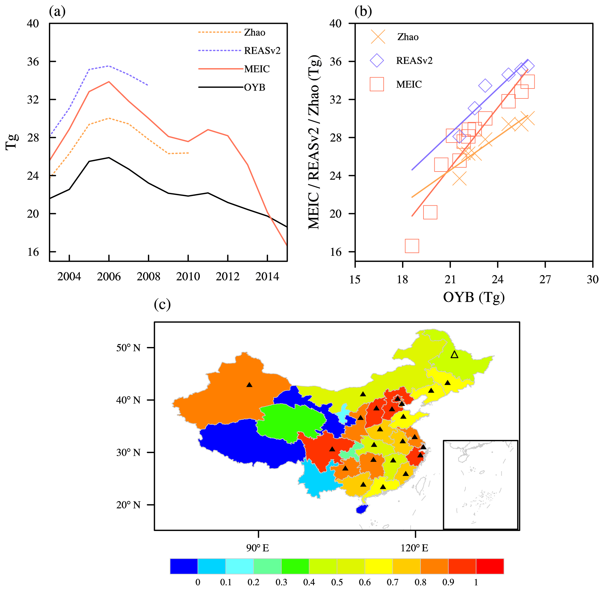
Figure 1(a) National total SO2 emissions estimated by OYB (solid black), MEIC (solid red), REAS (dashed blue) and Zhao (dashed orange) between 2003 and 2015. (b) Scatter diagrams and regression lines for the OYB estimate (x axis) against the other three products (y axis). (c) The province-by-province correlations between the OYB and MEIC products, with the significance levels of 0.1 and 0.05 being marked by open and filled triangles, respectively.
Figure 1 compares the OYB and MEIC emission inventories in terms of both national and regional scales. In addition, the other two candidates on national annual totals including REASv2 (Kurokawa et al., 2013) and Zhao (Xia et al., 2016) are overlaid. Figure 1a shows that considerable differences exist with regards to the magnitude among the four datasets and, in particular, OYB emissions are generally lower than those deduced from other inventories. However, their temporal variations are characterized in a very similar manner. As further illustrated in the scatter plot of OYB against the other three (Fig. 1b), highly linear clustered markers with correlations above 0.92 confirm such temporal consistency. On an even smaller regional scale, as shown in Fig. 1c, high degrees of correspondence between OYB and MEIC overwhelm the whole of East China, with most correlations exceeding the 0.05 significance level. In comparison, West China features relatively less agreement, but it is not a major concern in this study.
In short, all the datasets capture coherent temporal behaviors, despite the spread in their magnitudes. We emphasize that this study is centered on the fluctuation patterns rather than the magnitude itself. Therefore, the above evidence justifies the use of the OYB dataset in the following text. Meanwhile, in order to test whether results were robust to using a different dataset, all analyses have been repeated using the MEIC inventory.
2.3 Meteorological fields
The large-scale meteorological conditions are taken from Japanese 55-year Reanalysis (JRA-55) data, prepared by the Japan Meteorological Agency (Kobayashi et al., 2015; Harada et al., 2016). The variables analyzed include total column precipitable water, horizontal wind and temperature at pressure levels.
3.1 Mean distribution
Based on 12 years of SO2 column data over China, Fig. 2a shows the spatial pattern of the long-term mean. Overall, SO2 distribution is of great inhomogeneity in China, with two maximum centers: one is the North China Plain (NCP for short), and the other is Cheng-Yu (CY) district in Southwest China. In particular, the SO2 amount in the NCP exceeds 1.2 DU. There are two essential causes responsible for high SO2 loading in the two areas. On the one hand, the combined effect of rapid economic and industrial development as well as population growth leads to a high degree of anthropogenic SO2 emission. Figure 2c and d show the emission strengths, defined as emitted SO2 per unit area, in each province based on OYB and MEIC, respectively. Note that in the rest of this paper, the terms “emission” or “emission amount” always refer to “per unit area emission”. It is obvious that the two regions release above 8.0 t km−2 SO2 per year, which is 3 times greater than the average level of China. Although OYB exhibits a smaller magnitude of emissions than MEIC, the spatial patterns in terms of relative difference across space are generally consistent. On the other hand, as shown in Fig. 2b, either of the two regions is surrounded or partly surrounded by mountains, which makes it difficult for the pollutants to dissipate.
In contrast, over the sparsely populated western part of China, low SO2 concentrations of less than 0.2 DU are observed, except over some provincial capitals. Since the western part of China is less affected by human activities, anthropogenic sources of SO2 are much smaller than natural emissions including emissions from terrestrial ecosystems and oxidation of H2S to SO2 (Wang, 1999). Between latitude 30 and 40∘ N, for example, the SO2 amounts over the eastern regions (110–120∘ E) are 6–12 times greater than western regions (80–110∘ E). In addition, note that the low-level SO2 columns in West China are subject to large uncertainties and the background correction is an important source of error. However, West China with weak SO2 signals/background SO2 is not the subject of the present work, since we mainly focus on highly polluted East China.
Besides the NCP and CY regions with the highest SO2 loadings, this study is also interested in the Yangtze River Delta (YRD) and Pearl River Delta (PRD), the other two economic mega-urban zones in China. These four identified hotspots NCP, CY, YRD and PRD are outlined in Fig. 2a and will be specially examined in the following discussion.
3.2 Seasonal cycle
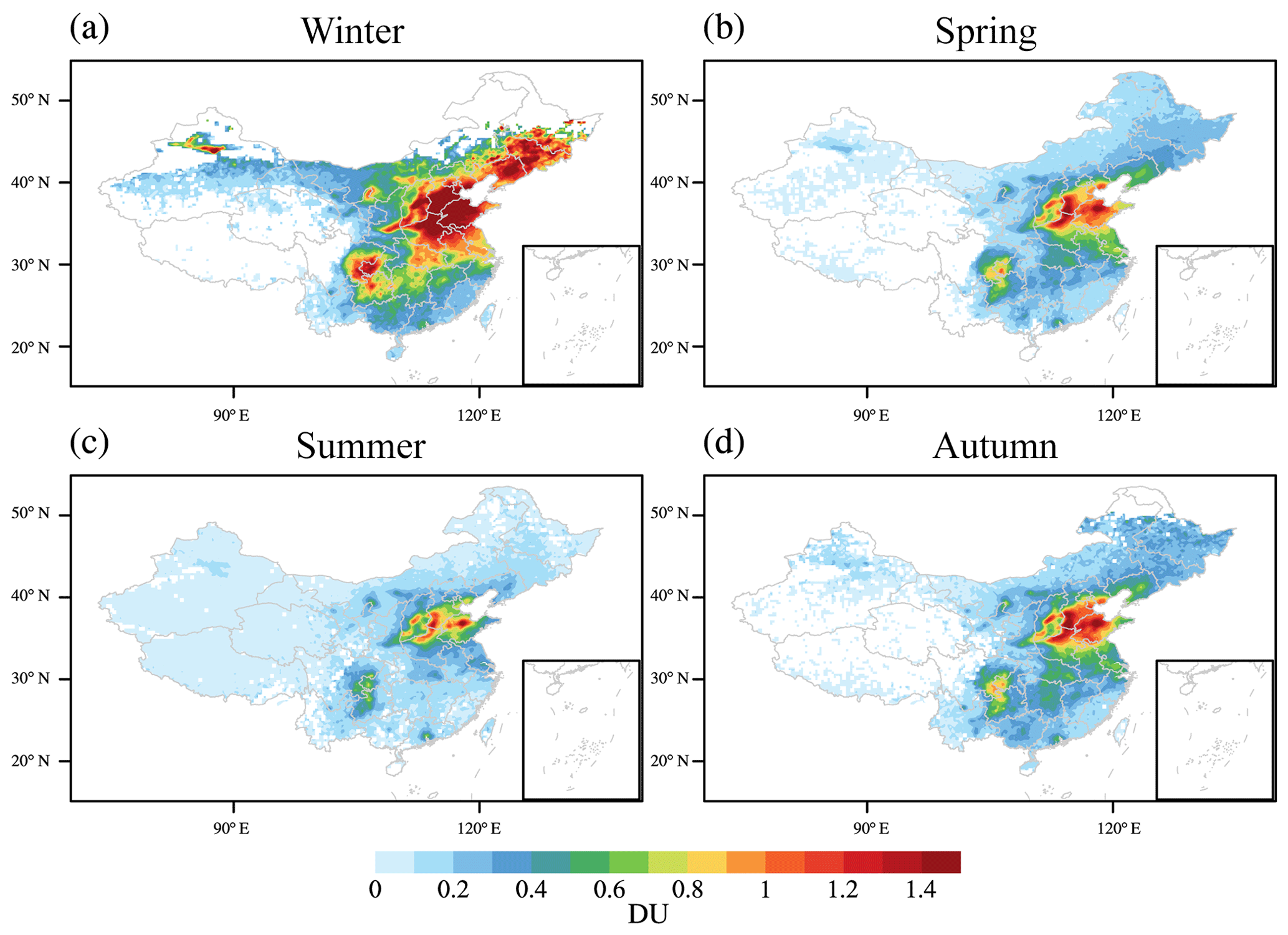
The annual total is decomposed into the seasonal cycle, as shown in Fig. 3. In East China, about 35 % of the annual total is from winter, while SO2 in summer only accounts for 15 %; the remaining 50 % is almost equally divided into spring and autumn. Seasonal variations measured in the fractional contribution are similar within East China.
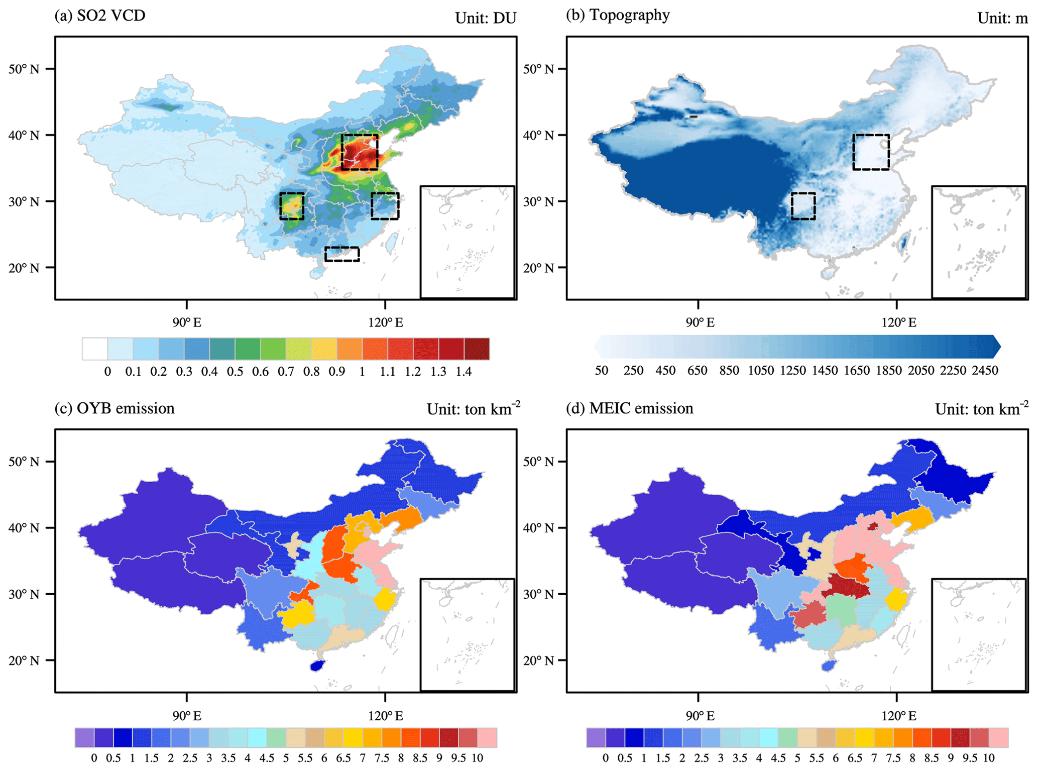
Figure 2(a) Spatial distribution of 12-year (2005–2016) averaged SO2 columns over China. (b) Topography of China in meters. (c, d) SO2 emission (t km−2) among Chinese provinces based on OYB and MEIC.
To unveil the underlying mechanism, Fig. 4 illustrates the annual cycle of SO2 VCDs in relation to sulfur emission, precipitable water and temperature at the four hotspots. Intensive heating during winter in North China raises sulfur release. However, emissions alone are not sufficient to explain the pronounced seasonality of SO2. The remaining variation is associated with the seasonal change in the meteorological conditions. Temperature and humidity are cold and dry in winter due to the influence of winter monsoon, and jointly weaken the rate of oxidation and wet deposition. Thus, one expects that SO2 molecules will have a longer lifetime and therefore will accumulate more easily. The opposite is true for summer, when chemical reaction is active and wet removal is effective. In summary, both emission and meteorological change explain the seasonality of the atmospheric SO2 loadings.
Due to the climate transition from South China to North China, the annual range of SO2 rises progressively from south to north. NCP has the greatest amplitude of up to 1 DU, while there is virtually no annual cycle in PRD. A larger amplitude for SO2 cycles in NCP arises from the significantly reversed source–sink imbalance between summer and winter. In contrast, the climate in PRD is characterized by a smoother transition over the whole year and there is no heating season, which explains the insignificant seasonal variation of SO2 in PRD. The other two regions, CY and YRD, have approximately the same amplitude of 0.6 DU, because they are on the same line of latitude.
3.3 Long-term trends
Figure 5 depicts the spatial pattern of linear trends in annual and seasonal SO2 from 2005 to 2016. Overall, apparent downward trends overwhelm most parts of East China, while West China has experienced little change. In particular, the most significant reduction occurred in the highly SO2-polluted regions, with the decreasing rates amounting to 0.1 DU a−1. This result suggests that the governments and communities in these economically developed regions have done their best to effectively control environmental pollution, including energy saving, emission cut, adjustment of energy consumption structure, shutdown of the most polluting factories, and upgrade of coal quality. Besides, enforcement of environmental protection laws is becoming more and more rigorous (van der A et al., 2017). Therefore, under collaborative efforts, the SO2 levels in these highly developed regions with high background concentrations have been decreasing markedly in the last decade. Moreover, the pattern correlation between mean (Fig. 2a) and trends (Fig. 5a) of SO2 reaches −0.77, implying that the downward rate over China can be summarized into a general rule – the higher the SO2 loading, the more significant the decrease.
Figure 5b–e portray the long-term trends of SO2 on a seasonal basis. On the one hand, every season has witnessed SO2 reduction, with the strongest decrease occurring in winter and autumn. Consequently, it can be concluded that the SO2 decreases in winter and autumn contribute most to the reduction of annual SO2. On the other hand, the highly SO2-polluted regions have experienced the most pronounced decrease across all seasons, which is consistent with the annual outcomes. It is worth pointing out that a belt of large positive values extends along 40∘ N in winter (Fig. 5b). This feature is a known artefact related to the large solar zenith angles at high northern latitudes.
Last, we discuss the trends of the four hotspots involved. Figure 6 depicts the SO2 columns from 2005 to 2016 as a function of year (y axis) and calendar month (x axis). The horizontal axis is the month of the year, the vertical axis is the year, and the color is the SO2 VCD for that month and year. SO2 VCDs exhibit a decreasing tendency during the last decade, regardless of the time of the year. Quantitatively, SO2 in NCP, CY, YRD and PRD had undergone an overall downward trend with a rate of 0.062, 0.059, 0.046 and 0.055 DU per year, respectively.
4.1 Specific regimes of SO2 variability
The above investigation presents SO2 patterns and trends across China, but some elusive non-monotonic behaviors are not fully understood. In this section, we aim to detect the specific regimes of SO2 variability and associated responsible mechanisms.

Figure 4Annual cycle of SO2 VCD (unit: DU, pink line), MEIC SO2 emission (unit: t km−2, yellow line), precipitable water (unit: kg m−2, blue bar) and temperature at 925 hPa (unit: ∘C, green line) for NCP (a), CY (b), YRD (c) and PRD (d).
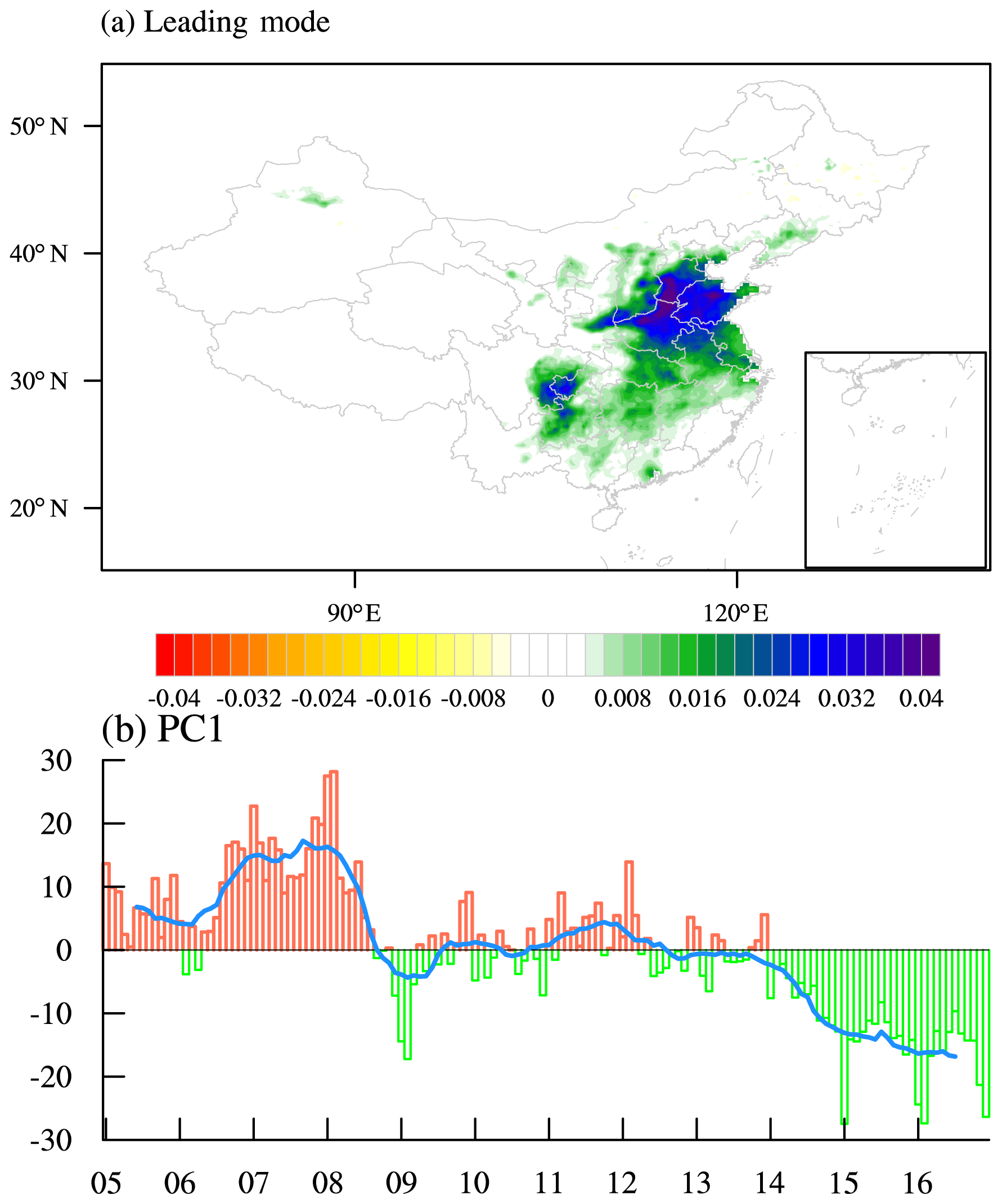
Spatiotemporal regimes of SO2 over China are mapped by using empirical orthogonal function (EOF) decomposition (Hannachi, 2004), which is a useful tool to reduce the data dimensionality to two dimensions. One dimension represents the spatial structure and the other the temporal dimension. Figure 7 illustrates the leading mode (top) and the corresponding principal component (PC, bottom) obtained from EOF, since only the first mode is statistically well separated. Compared to the first EOF mode explaining 36.8 % of the total variance, each of the other modes is characterized by less than 6 % contribution and is thus discarded. On the one hand, the variation of SO2 is dominated by a spatially uniform feature with large loadings in NCP and CY, suggesting that SO2 changes would be in the same phase but with varying amplitude across the entire region. On the other hand, the corresponding PC exhibits overall declines during 2005 to 2016. However, the result does not imply a simple continuous decrease. In fact, there appears to be a transient increase until a peak and thereafter two sharp drops occur in the periods 2007–2008 and 2014–2016, amid which SO2 concentrations are in the process of slightly rebounding. In short, the SO2 variability is characterized by four distinct temporal regimes.
Moreover, Fig. 8 demonstrates the time series for each province in East China, with the segment over 2009–2013 highlighted by red color. It reflects extensive common variation that goes through four stages – that is, a short-lived increasing period at the beginning, a steep drop period during 2007 to 2008, a rebound period of 2009 to 2013 and another drastic drop period during 2014 to 2016. Most importantly, it confirms that the SO2 does not evolve in a monotonic way but shows a striking rebound during 2009 to 2013. This pattern is true throughout most of the region, with the only two exceptions of Guizhou and Guangdong provinces, which have experienced a continuous decrease since 2005.
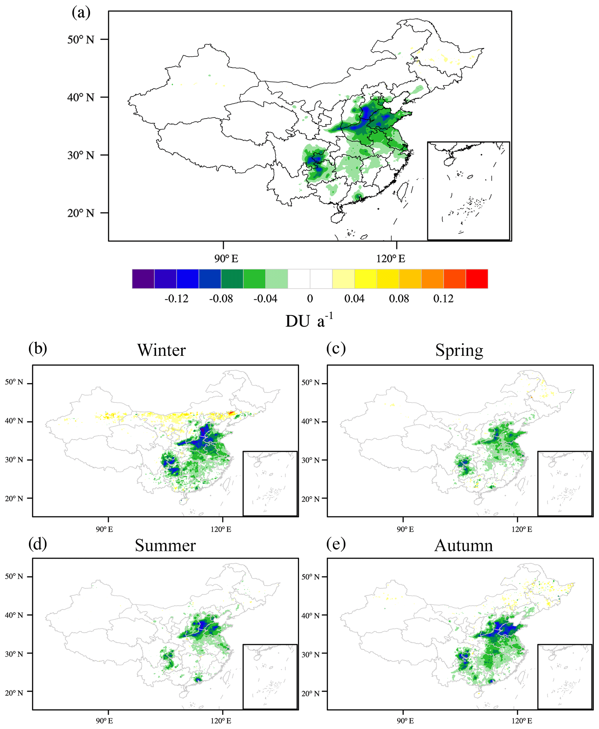
Figure 5Spatial pattern of SO2 linear trends (2005–2016) in annual (a) and seasonal (b–e) values.
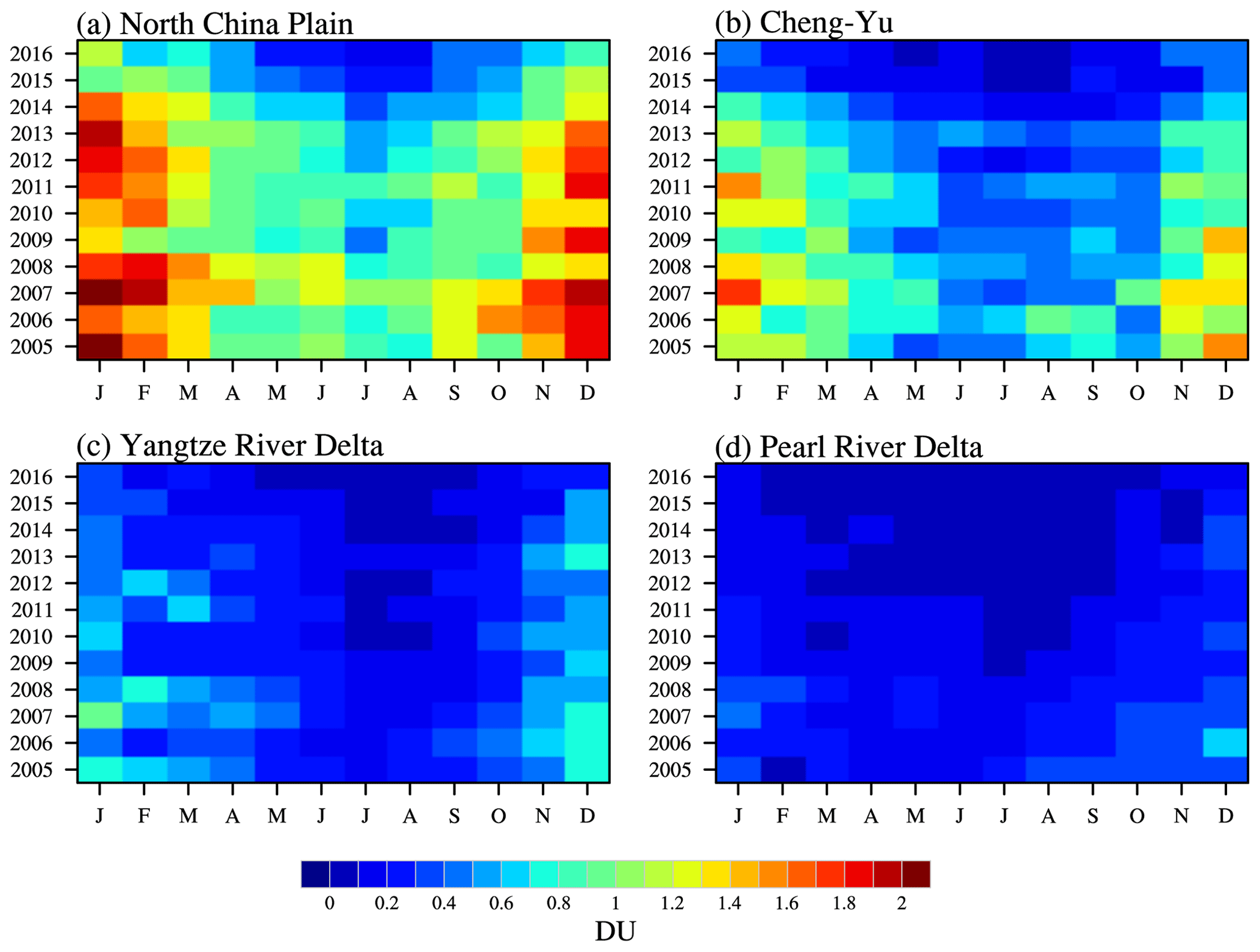
Figure 6SO2 amounts from 2005 to 2016 as a function of year (y axis) and calendar month (x axis) for NCP (a), CY (b), YRD (c) and PRD (d).
4.2 Causes
In this section, we diagnose the likely mechanisms behind the observed SO2 variability. Generally, emissions and meteorological conditions are two main factors that essentially exert influence on atmospheric pollutant load. The impact of changes in emitted SO2, as the main driving force, is first examined. To this end, the temporal classifications of SO2 emission for each province based on OYB and MEIC are, respectively, depicted in Fig. 9a and b, in which the red upward pointing triangle implies non-monotonic decrease with a rebound in the middle, whereas persistent decrease is denoted by the green downward pointing triangle. In North China except Henan province, both the OYB and MEIC datasets show that the emission passed its secondary peak during 2009 to 2013. In South China, however, discrepancies between OYB and MEIC emerge in some provinces, namely Jiangxi, Hunan, Guangxi and Guizhou. Even so, we are still confident enough that the majority of South China has witnessed a successive drop in emitted SO2. In addition, an auxiliary map is presented in Fig. 9c showing the slope of the linear regression of MEIC gridded emission over years 2008, 2010 and 2012. We can see that most of North China is subject to a positive rate of change, while the opposite holds true over most of South China, which confirms the above findings. Eventually, we come to the conclusion that despite spatial uniformity in temporal-pattern classification of SO2 VCD (Fig. 8), the temporal structure of the emission demonstrates a strong south–north contrast (Fig. 9). Therefore, it is advantageous to treat North China and South China separately, as delineated by the dotted line in Fig. 9. Regional averaged quantities are estimated as a weighted average by assigning the district area as a weight. In addition, to evade possible contaminations, we have ruled out Henan and Jiangxi provinces in OYB and Henan, Hunan, Guizhou and Guangxi provinces in MEIC.
Although we divide East China into north and south blocks, the inter-regional transport cannot be neglected. Therefore, we construct an Effective Emission Index (EEI) to account for impacts from both local and remote sources. Here, we directly adopt the results obtained by Zhang et al. (2015), who divided East China into three parts, North China, Southeast China and Southwest China, and quantified the percent contributions of within-region versus inter-regional transport on sulfate concentrations. The geographical partition in their work broadly coincides with ours, with the only difference that South China is further split into two parts. Given that the ratio of Southeast China to Southwest China is 1.4, we merge the percent contributions over these two portions via simple conversions. This produces, for North China, a within-region SO2 emission contribution of 68 %, followed by 19 % from South China and 13 % from other regions; for South China, within-region emissions provide 66 %, while transport from North China and other regions amounts to 17 % and 17 %, respectively. With these statistics, the EEI is formulated as follows.
| North China | EEI |
| EEI |
| South China | EEI |
| EEI | |
N and S denote the emission amount in North China and South China, respectively, and subscripts 1 and m the 1st and mth time node, respectively. The fundamental assumptions to derive the formula are that EEI is linearly dependent on N and S and the external contributions remain fixed (without interannual variation). For comparison purposes, we also define an Emission Index (EI) that involves a single effect from within-region emission, as written below.
| North China | EI1=1 |
| EI |
| South China | EI1=1 |
| EI | |
The notations of symbols are identical to those in the EEI definition. In the case of a large scale, integrating the role of inter-regional transport does not alter the overall pattern, as proved in the following analyses.
Figure 10 presents time series and scatter plots of SO2 VCD and emission with its variants EI and EEI, and Fig. 11 is designed to show the total emission generated by industries and households. These two figures are created based on the OYB inventory, while their counterparts obtained from the MEIC inventory are shown in Figs. S3 and S4. As shown in Fig. 10a, North China features a good correspondence between amount and either EI or EEI, with a linear correlation of 0.9. Time series of emission also indicate the existence of four distinct regimes that are likely to drive the regime of SO2 VCD directly. This is confirmed by the scatter plot (Fig. 10b), in which the points are tightly clustered around the regression line. Based on variance analysis, emission accounts for an 81 % fraction of SO2 VCD variation over North China. In parallel, the same procedure relying on the MEIC inventory yields nearly identical results, as shown in Fig. S3a and b. Furthermore, how large do industrial and household sectors, respectively, contribute to the total trends? Figures 11a and S4a indicate that the industrial emissions play a crucial role in SO2 VCD variation throughout the whole period, while the influence induced by residential activity is secondary. A more in-depth comparison between OYB and MEIC shows some dissimilarity in household emission: OYB-based household emission acts to offset the industrial effect, while the opposite function is identified for the MEIC-based one. However, this does not seriously affect the major conclusion, due to the marginal impacts caused by households.
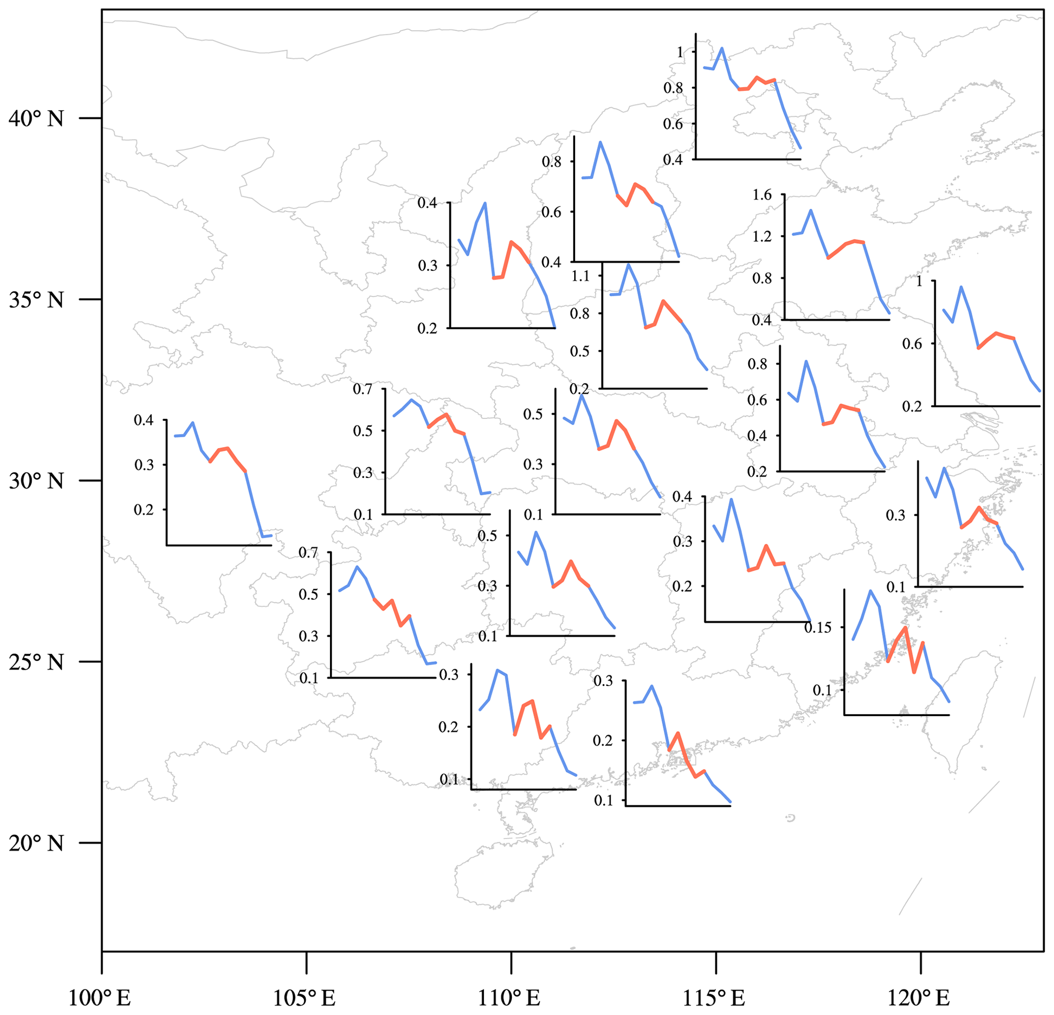
Figure 8Temporal evolution of annual SO2 (unit: DU) from 2005 to 2016 in each province of eastern China, with the segment over 2009–2013 highlighted by red color.
The close linear relationship observed in North China is not found in South China, since the two curves appear to become non-adherent in Fig. 10c and the points in the scatter plot Fig. 10d are widely spread around the regression line. Variance analysis suggests that only 45 % of SO2 VCD variability is forced by emissions, suggesting that the SO2 variations in South China cannot be explained by emission changes alone. This is mainly ascribed to the decoupled pathways of emission and SO2 VCD during 2009 to 2013, as the emission continues to decline but SO2 VCD witnesses a rebound. MEIC emissions also exhibit a general decreasing tendency in spite of a transient pause embedded, as shown in Fig. S3c. Moreover, Figs. 11b and S4b suggest that the cuts of industrial and household emissions collectively promote the continuous decrease in total emission in South China, which are different from that in North China. However, the emission decrease in the household sector is differently reported in the OYB and MEIC inventories, the former one showing a sudden shift, while the latter displays a gradual decrease. Anyway, one is assured that household emissions in South China have undergone a reduction, irrespective of the exact manner.
Why do decreasing emissions not cause a reduction of SO2 VCD in South China during 2009 to 2013? To answer this question, the atmospheric conditions during 2009 to 2013 are compared with those during the rest of the years, as depicted in Fig. 12. The period 2009 to 2013 is characterized by prolonged dry conditions in South China with the precipitable water and precipitation being lower than usual (Fig. 12a), which weakens wet adsorption and scavenging. At the same time, this period is also associated with relatively weaker wind speed (Fig. 12b) and increased static stability (Fig. 12c and d), reducing the ability of the atmosphere to diffuse, leading to the accumulation of SO2 loads. In brief, unfavorable meteorological conditions produce the observed rebound of SO2 during 2009 to 2013, despite the continued decrease in emission.
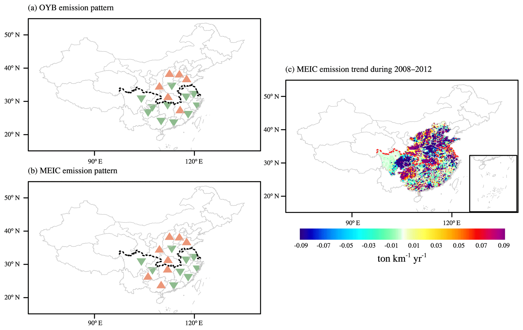
Figure 9(a, b) Temporal structure classification of SO2 emission based on OYB and MEIC. Red upward pointing triangles imply non-monotonic decrease with a rebound in the middle, while monotonic decrease is denoted by green downward pointing triangles. (c) Slope of the linear regression of MEIC gridded emission over years 2008, 2010 and 2012. The black or red dotted line delimits North China and South China.
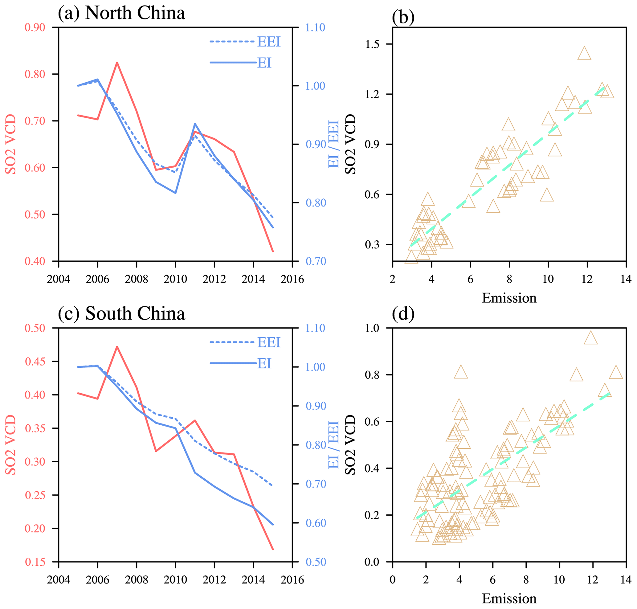
Figure 10Time series plots of SO2 VCD and EI/EEI (a, c), and scatter plots with the regression line of SO2 VCD and emission (b, d) for North China (a, b) and South China (c, d). Each marker in (b) and (d) corresponds to one year and one province.
In this study, the spatiotemporal variability of SO2 columns over China and the associated driving mechanisms are examined over the past decade. Based on a state-of-the-art SO2 retrieval dataset recently derived from the OMI, we elaborate on the characteristics of specific SO2 regimes over China and underlying causes.
Climatological SO2 in China has an uneven spatial distribution in space and time. East China is far more exposed to SO2 pollution than West China, with two maxima centered in NCP and CY. From analysis of the annual cycles we conclude that 35 % of the annual totals are from winter, while SO2 in summer only accounts for 15 %. In addition, the annual amplitude of SO2 rises progressively from south to north.

Figure 11Annual SO2 emission (t km−2) generated by industries (upward blue bars) and households (downward red bars) in North China (a) and South China (b). Note that the y axis in a positive direction does not start at zero.
From 2005 through 2016, most of East China presents a clear decreasing tendency for SO2, while West China experiences little change. Spatially, the decreasing rate is generally enhanced for high SO2 loads. When computed seasonally, SO2 reductions in winter and autumn contribute most to the reduction of annual SO2.
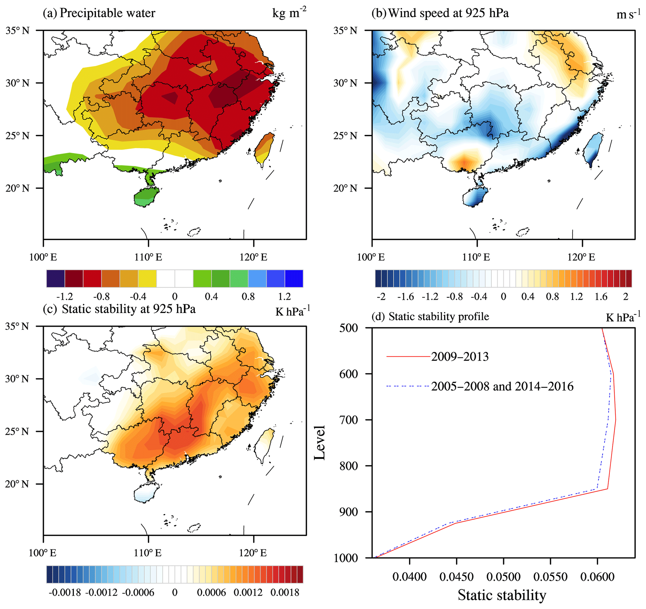
Figure 12Comparison of atmospheric conditions between the period of 2009–2013 and the other years: (a) composite difference in precipitable water (unit: kg m−2), (b) composite difference in wind velocity at 925 hPa (unit: m s−1), (c) composite difference in static stability at 925 hPa (unit: K hPa−1), and (d) averaged vertical profile of static stability over the 23–31∘ N, 105–122∘ N rectangle for the two episodes.
Four stages of variation are identified by EOF analysis. The first regime (2005–2006) features a transient increasing trend, the second (2007–2008) and the last (2014–2016) regimes show sharp drops, and the third regime (2009–2013) manifests itself in 5-year moderate rebounding. Although temporal regimes of SO2 are coherent throughout the country, different driving forces are tied to North China and South China. In North China, the atmospheric SO2 and emission vary essentially in the same way. Therefore, the atmospheric SO2 variability is primarily associated with the emission variability, which accounts for 81 % of the total variance. Further, the emission generated by the industrial sector is largely responsible for the atmospheric SO2 variability. The household emissions appear to remain uncertain, due to the dissimilarity between the OYB and MEIC inventories.
SO2 emissions in South China exhibit a continuous decreasing tendency, due to the coordinated cuts of industrial and household emissions. As a result, the role of emissions only contributes 45 % of the SO2 variation, primarily owing to the decoupled pathways of emission and atmospheric content during 2009 to 2013 when the emission continues to decline but atmospheric content witnesses a rebound. It is found that such rebound occurs in response to the joint effect of deficient precipitation, weaker wind speed and increased static stability during 2009 to 2013.
As shown by this study, the spatial and temporal changes in SO2 regimes over China in the recent decade become clear. However, there is much left to be learned about the responsible driving mechanisms. First, a major obstacle to cause-and-effect relation surveys stems from uncertainties in the current emission inventories. In this study, many facets inferred by OYB and MEIC are convergent, because we look at a large spatial scale and long-term general tendency that help filter out or attenuate some uncertainties. However, if the aim is to focus on smaller spatial or temporal scales or on specific sectors, there is still great uncertainty. To overcome these barriers, emission inventories should be further improved and more observational products should be used for comparison. Second, this work investigates the impact of emission, inter-regional transport and meteorology using purely statistical techniques, but finer-scale investigations require numerical simulations using coupled chemical-transport models. Third, the analysis presented in Sect. 4 is constrained to provincial or multi-provincial levels, due to the limitation that only continuous emission data on provinces are gathered at hand. In reality, however, either emission or atmospheric loadings can be quite inhomogeneous within the same region. Therefore, future studies should use both gridded SO2 VCDs and gridded SO2 emission inventories.
The BIRA SO2 product can be obtained by contacting co-author Nicolas Theys. The OYB emission inventory is publicly available at the National Bureau of Statistics of China webpage http://www.stats.gov.cn/ztjc/ztsj/hjtjzl/ (NBS, 2003–2015). The MEIC emission inventory can be made available upon request to co-author Qiang Zhang or through the MEIC homepage http://www.meicmodel.org/ (M. Li et al., 2017). The Zhao emission inventory is provided in the supplement of Xia et al. (2016). The REASv2 emission inventory is publicly accessible via https://www.nies.go.jp/REAS/index.html (Kurokawa et al., 2013). The JRA-55 reanalysis data can be downloaded from ftp://ds.data.jma.go.jp/ (Kobayashi et al., 2015).
The supplement related to this article is available online at: https://doi.org/10.5194/acp-18-18063-2018-supplement.
TW conducted the majority of data analysis and drafted the manuscript. NT developed the BIRA SO2 product, with collaboration from FH. DT and QZ prepared MEIC emission inventory data. PW and MVR are principal investigators of this study, responsible for the overall structure, design and paper writing. All co-authors contributed toward revising and improving the manuscript.
The authors declare that they have no conflict of interest.
We are grateful to the editor and two anonymous reviewers for constructive
comments and suggestions that greatly improved the quality of this paper.
This work was supported by the National Key Research and Development Program
of China nos. 2017YFB0504000 and 2016YFC0200403, and the National Natural
Science Foundation of China nos. 41505021 and 41575034.
Edited by: Dominick Spracklen
Reviewed by:
Yang Wang and one anonymous referee
Chai, F., Gao, J., Chen, Z., Wang, S., Zhang, Y., Zhang, J., Zhang, H., Yun, Y., and Ren, C.: Spatial and temporal variation of particulate matter and gaseous pollutants in 26 cities in China, J. Environ. Sci., 26, 75–82, 2014.
Chan, C. K. and Yao, X.: Air pollution in mega cities in China, Atmos. Environ., 42, 1–42, 2008.
Hannachi, A.: A primer for EOF analysis of climate data, University of Reading, Reading, 2004.
Harada, Y., Kamahori, H., Kobayashi, C., Endo, H., Kobayashi, S., Ota, Y., Onoda, H., Onogi, K., Miyaoka, K., and Takahashi, K.: The JRA-55 Reanalysis: Representation of atmospheric circulation and climate variability, J. Meteorol. Soc. Jpn. Ser. II, 94, 269–302, 2016.
Hou, Y., Wang, L., Zhou, Y., Wang, S., and Wang, F.: Analysis of the Sulfur Dioxide Column Concentration over Jing-Jin-Ji, China, based on Satellite Observations during the Past Decade, Polish J. Environ. Stud., 27, 1551–1557, 2018.
Jin, J., Ma, J., Lin, W., Zhao, H., Shaiganfar, R., Beirle, S., and Wagner, T.: MAX-DOAS measurements and satellite validation of tropospheric NO2 and SO2 vertical column densities at a rural site of North China, Atmos. Environ., 133, 12–25, 2016.
Kobayashi, S., Ota, Y., Harada, Y., Ebita, A., Moriya, M., Onoda, H., Onogi, K., Kamahori, H., Kobayashi, C., Endo, H., Miyaoka, K., and Takahashi, K.: The JRA-55 reanalysis: General specifications and basic characteristics, J. Meteorol. Soc. Jpn. Ser. II, 93, 5–48, https://doi.org/10.2151/jmsj.2015-001, 2015.
Koukouli, M. E., Balis, D. S., Theys, N., Hedelt, P., Richter, A., Krotkov, N., Li, C., and Taylor, M.: Anthropogenic sulphur dioxide load over China as observed from different satellite sensors, Atmos. Environ., 145, 45–59, 2016.
Krotkov, N. A., McLinden, C. A., Li, C., Lamsal, L. N., Celarier, E. A., Marchenko, S. V., Swartz, W. H., Bucsela, E. J., Joiner, J., Duncan, B. N., Boersma, K. F., Veefkind, J. P., Levelt, P. F., Fioletov, V. E., Dickerson, R. R., He, H., Lu, Z., and Streets, D. G.: Aura OMI observations of regional SO2 and NO2 pollution changes from 2005 to 2015, Atmos. Chem. Phys., 16, 4605–4629, https://doi.org/10.5194/acp-16-4605-2016, 2016.
Kurokawa, J., Ohara, T., Morikawa, T., Hanayama, S., Janssens-Maenhout, G., Fukui, T., Kawashima, K., and Akimoto, H.: Emissions of air pollutants and greenhouse gases over Asian regions during 2000–2008: Regional Emission inventory in ASia (REAS) version 2, Atmos. Chem. Phys., 13, 11019–11058, https://doi.org/10.5194/acp-13-11019-2013, 2013.
Lee, C., Martin, R. V., Van Donkelaar, A., Lee, H., Dickerson, R. R., Hains, J. C., Krotkov, N., Richter, A., Vinnikov, K., and Schwab, J. J.: SO2 emissions and lifetimes: Estimates from inverse modeling using in situ and global, space-based (SCIAMACHY and OMI) observations, J. Geophys. Res.-Atmos., 116, D06304, https://doi.org/10.1029/2010JD014758, 2011.
Levelt, P. F., Van den Oord, G. H. J., Dobber, M. R., Malkki, A., Visser, H., de Vries, J., Stammes, P., Lundell, J. O. V., and Saari, H.: The ozone monitoring instrument, IEEE T. Geosci. Remote, 44, 1093–1101, 2006.
Li, C., Zhang, Q., Krotkov, N. A., Streets, D. G., He, K., Tsay, S. C., and Gleason, J. F.: Recent large reduction in sulfur dioxide emissions from Chinese power plants observed by the Ozone Monitoring Instrument, Geophys. Res. Lett., 37, L08807, https://doi.org/10.1029/2010GL042594, 2010.
Li, C., Joiner, J., Krotkov, N. A., and Bhartia, P. K.: A fast and sensitive new satellite SO2 retrieval algorithm based on principal component analysis: Application to the ozone monitoring instrument, Geophys. Res. Lett., 40, 6314–6318, 2013.
Li, C., McLinden, C., Fioletov, V., Krotkov, N., Carn, S., Joiner, J., Streets, D., He, H., Ren, X., Li, Z., and Dickerson, R. R.: India is overtaking China as the world's largest emitter of anthropogenic sulfur dioxide, Scient. Rep., 7, 14304, https://doi.org/10.1038/s41598-017-14639-8, 2017.
Li, M., Liu, H., Geng, G., Hong, C., Liu, F., Song, Y., Tong, D., Zheng, B., Cui, H., Man, H., Zhang, Q., and He, K.: Anthropogenic emission inventories in China: a review, Nat. Sci. Rev., 4, 834–866, https://doi.org/10.1093/nsr/nwx150, 2017.
Lin, W., Xu, X., Ma, Z., Zhao, H., Liu, X., and Wang, Y.: Characteristics and recent trends of sulfur dioxide at urban, rural, and background sites in North China: Effectiveness of control measures, J. Environm. Sci., 24, 34–49, 2012.
Lu, Z., Streets, D. G., Zhang, Q., Wang, S., Carmichael, G. R., Cheng, Y. F., Wei, C., Chin, M., Diehl, T., and Tan, Q.: Sulfur dioxide emissions in China and sulfur trends in East Asia since 2000, Atmos. Chem. Phys., 10, 6311–6331, https://doi.org/10.5194/acp-10-6311-2010, 2010.
Ma, J., Xu, X., Zhao, C., and Yan, P.: A review of atmospheric chemistry research in China: Photochemical smog, haze pollution, and gas-aerosol interactions, Adv. Atmos. Sci., 29, 1006–1026, 2012.
Meng, X. Y., Wang, P. C., Wang, G. C., Yu, H., and Zong, X. M.: Variation and transportation characteristics of SO2 in winter over Beijing and its surrounding areas, Clim. Environ. Res., 14, 309–317, 2009.
MEPC – Ministry of Environmental Protection of China: Technical regulation on ambient air quality index (on trial), available at: http://kjs.mee.gov.cn/hjbhbz/bzwb/jcffbz/201203/t20120302_224166.shtml (last access: 10 December 2018), 2012.
Munro, R., Eisinger, M., Anderson, C., Callies, J., Corpaccioli, E., Lang, R., Lefebvre, A., Livschitz, Y., and Albinana, A. P.: GOME-2 on MetOp, in: Proc. of The 2006 EUMETSAT Meteorological Satellite Conference, Helsinki, Finland, 2006.
NBS – National Bureau of Statistics of China: China Statistical Yearbook on Environment, China Statistics Press, Beijing, available at: http://www.stats.gov.cn/ztjc/ztsj/hjtjzl/ (last access: December 2018), 2003–2015.
Ren, L., Yang, W., and Bai, Z.: Characteristics of Major Air Pollutants in China, in Ambient Air Pollution and Health Impact in China, Springer, Singapore, 7–26, 2017.
Rix, M., Valks, P., Hao, N., Loyola, D., Schlager, H., Huntrieser, H., Flemming, J., Koehler, U., Schumann, U., and Inness, A.: Volcanic SO2, BrO and plume height estimations using GOME-2 satellite measurements during the eruption of Eyjafjallajökull in May 2010, J. Geophys. Res.-Atmos., 117, D00U19, https://doi.org/10.1029/2011JD016718, 2012.
Su, S., Li, B., Cui, S., and Tao, S.: Sulfur dioxide emissions from combustion in China: from 1990 to 2007, Environ. Sci. Technol., 45, 8403–8410, 2011.
Theys, N., De Smedt, I., van Gent, J., Danckaert, T., Wang, T., Hendrick, F., Stavrakou, T., Bauduin, S., Clarisse, L., Li, C., Krotkov, N., Yu, H., Brenot, H., and Van Roozendael, M.: Sulfur dioxide vertical column DOAS retrievals from the Ozone Monitoring Instrument: Global observations and comparison to ground-based and satellite data, J. Geophys. Res.- Atmos., 120, 2470–2491, 2015.
van der A, R. J., Mijling, B., Ding, J., Koukouli, M. E., Liu, F., Li, Q., Mao, H., and Theys, N.: Cleaning up the air: effectiveness of air quality policy for SO2 and NOx emissions in China, Atmos. Chem. Phys., 17, 1775–1789, https://doi.org/10.5194/acp-17-1775-2017, 2017.
Wang, M.: Atmospheric Chemistry, 2nd Edn., China Meteorological Press, Beijing, 1999.
Wang, S., Zhang, Q., Martin, R. V, Philip, S., Liu, F., Li, M., Jiang, X., and He, K.: Satellite measurements oversee China's sulfur dioxide emission reductions from coal-fired power plants, Environ. Res. Lett., 10, 114015, https://doi.org/10.1088/1748-9326/10/11/114015, 2015.
Wang, T., Hendrick, F., Wang, P., Tang, G., Clémer, K., Yu, H., Fayt, C., Hermans, C., Gielen, C., Müller, J.-F., Pinardi, G., Theys, N., Brenot, H., and Van Roozendael, M.: Evaluation of tropospheric SO2 retrieved from MAX-DOAS measurements in Xianghe, China, Atmos. Chem. Phys., 14, 11149–11164, https://doi.org/10.5194/acp-14-11149-2014, 2014.
Wang, Y., Beirle, S., Lampel, J., Koukouli, M., De Smedt, I., Theys, N., Li, A., Wu, D., Xie, P., Liu, C., Van Roozendael, M., Stavrakou, T., Müller, J.-F., and Wagner, T.: Validation of OMI, GOME-2A and GOME-2B tropospheric NO2, SO2 and HCHO products using MAX-DOAS observations from 2011 to 2014 in Wuxi, China: investigation of the effects of priori profiles and aerosols on the satellite products, Atmos. Chem. Phys., 17, 5007–5033, https://doi.org/10.5194/acp-17-5007-2017, 2017.
WHO – World Health Organization: Ambient (outdoor) air quality and health, available at: http://www.who.int/news-room/fact-sheets/detail/ambient-(outdoor)-air-quality-and-health, last access: 10 December 2018.
Xia, Y., Zhao, Y., and Nielsen, C.: Benefits of China's efforts in gaseous pollutant control indicated by the bottom-up emissions and satellite observations 2000–2014, Atmos. Environ., 136, 43–53, 2016.
Yan, H., Chen, L., Su, L., Tao, J., and Yu, C.: SO2 columns over China: Temporal and spatial variations using OMI and GOME-2 observations, IOP Conf. Ser.: Earth Environ. Sci., 17, 012027, https://doi.org/10.1088/1755-1315/17/1/012027, 2014.
Yan, S. and Wu, G.: SO2 Emissions in China–Their Network and Hierarchical Structures, Scient. Rep., 7, 46216, https://doi.org/10.1038/srep46216, 2017.
Yu, H., Wang, P., Zong, X., Li, X., and Lü, D.: Change of NO2 column density over Beijing from satellite measurement during the Beijing 2008 Olympic Games, Chinese Sci. Bull., 55, 308–313, 2010.
Zhang, Q. Q., Wang, Y., Ma, Q., Yao, Y., Xie, Y., and He, K.: Regional differences in Chinese SO2 emission control efficiency and policy implications, Atmos. Chem. Phys., 15, 6521–6533, https://doi.org/10.5194/acp-15-6521-2015, 2015.
Zhang, X., van Geffen, J., Liao, H., Zhang, P., and Lou, S.: Spatiotemporal variations of tropospheric SO2 over China by SCIAMACHY observations during 2004–2009, Atmos. Environ., 60, 238–246, 2012.
Zhang, Y., Li, C., Krotkov, N. A., Joiner, J., Fioletov, V., and McLinden, C.: Continuation of long-term global SO2 pollution monitoring from OMI to OMPS, Atmos. Meas. Tech., 10, 1495–1509, https://doi.org/10.5194/amt-10-1495-2017, 2017.
Zheng, B., Tong, D., Li, M., Liu, F., Hong, C., Geng, G., Li, H., Li, X., Peng, L., Qi, J., Yan, L., Zhang, Y., Zhao, H., Zheng, Y., He, K., and Zhang, Q.: Trends in China's anthropogenic emissions since 2010 as the consequence of clean air actions, Atmos. Chem. Phys., 18, 14095–14111, https://doi.org/10.5194/acp-18-14095-2018, 2018.