the Creative Commons Attribution 4.0 License.
the Creative Commons Attribution 4.0 License.
 | 18 Dec 2018
Meteorological conditions during the ACLOUD/PASCAL field campaign near Svalbard in early summer 2017
Bernd Heinold
Sandro Dahlke
Heiko Bozem
Susanne Crewell
Irina V. Gorodetskaya
Georg Heygster
Daniel Kunkel
Marion Maturilli
Mario Mech
Carolina Viceto
Annette Rinke
Holger Schmithüsen
André Ehrlich
Andreas Macke
Christof Lüpkes
Manfred Wendisch
The two concerted field campaigns, Arctic CLoud Observations Using airborne measurements during polar Day (ACLOUD) and the Physical feedbacks of Arctic planetary boundary level Sea ice, Cloud and AerosoL (PASCAL), took place near Svalbard from 23 May to 26 June 2017. They were focused on studying Arctic mixed-phase clouds and involved observations from two airplanes (ACLOUD), an icebreaker (PASCAL) and a tethered balloon, as well as ground-based stations. Here, we present the synoptic development during the 35-day period of the campaigns, using near-surface and upper-air meteorological observations, as well as operational satellite, analysis, and reanalysis data. Over the campaign period, short-term synoptic variability was substantial, dominating over the seasonal cycle. During the first campaign week, cold and dry Arctic air from the north persisted, with a distinct but seasonally unusual cold air outbreak. Cloudy conditions with mostly low-level clouds prevailed. The subsequent 2 weeks were characterized by warm and moist maritime air from the south and east, which included two events of warm air advection. These synoptical disturbances caused lower cloud cover fractions and higher-reaching cloud systems. In the final 2 weeks, adiabatically warmed air from the west dominated, with cloud properties strongly varying within the range of the two other periods. Results presented here provide synoptic information needed to analyze and interpret data of upcoming studies from ACLOUD/PASCAL, while also offering unprecedented measurements in a sparsely observed region.
- Article
(18597 KB) -
Supplement
(5290 KB) - BibTeX
- EndNote


The phenomenon of Arctic amplification – the 2–3 times higher warming of the Arctic relative to the global atmosphere – is a major indication of current drastic Arctic climate changes (Serreze and Barry, 2011). A number of potential causes for this special feature of the Arctic climate system are discussed, which include various interconnected processes and feedback mechanisms, such as sea ice loss and surface albedo feedback, meridional atmospheric and oceanic energy fluxes, and atmospheric radiation effects linked to temperature, water vapor, and clouds (Pithan and Mauritsen, 2014). Still, the relative importance of these different feedback mechanisms is subject of the current scientific debate (Wendisch et al., 2017).
Climate models have difficulties in reproducing the observed drastic Arctic climate changes, and therefore the uncertainty in Arctic climate projections is larger than in other parts of the world (Stocker et al., 2013). This issue is related to major gaps in understanding of key processes particularly important for the Arctic climate system. Significant uncertainties in the parameterization of subgrid-scale processes remain one of the major challenges for realistic climate simulations, particularly in high latitudes (Vihma et al., 2014). Further important open questions are associated with cloud physical processes (Pithan et al., 2014; Tjernström et al., 2008; de Boer et al., 2014) and sea ice albedo–cloud radiative interactions (English et al., 2015; Karlsson and Svensson, 2013). The results of different Arctic climate models substantially disagree; they also generally do not match with observations, in particular with respect to hydrometeor phase partitioning in mixed-phase clouds (McIlhattan et al., 2017; Morrison et al., 2011) and the vertical structure of the atmospheric boundary layer (Svensson and Lindvall, 2015), which are interrelated (Barton et al., 2014; Lüpkes et al., 2010; Pithan et al., 2014). Those biases can considerably affect the water vapor and temperature profiles and the atmospheric radiation budget, which can consequently alter the individual climate feedback (Kim et al., 2016). To make substantial progress in these areas, dedicated observational campaigns in the Arctic are crucial.
In this framework, a number of airborne and ship-based campaigns with a focus on Arctic aerosol–cloud–ABL processes were conducted within the last decade (Wendisch et al., 2018). However, most of these previous observational campaigns in the Arctic obtained relatively few process-level observations of the coupled Arctic climate system, especially related to interactions between clouds and the ABL and with regards to the radiative interaction of the cloud properties with the surface. And, although all these campaigns have been conducted in the last decade and thus measured the “new Arctic” (Jeffries et al., 2013), they are hard to compare due to the different synoptic and sea ice conditions as well as climate regimes in the various regions. Nevertheless, the comparison both with other campaigns and with the long-term observations of the land-based station Ny-Ålesund helps to estimate the representativeness of the measurements for the sea ice environment of the Arctic North Atlantic sector, and if/how the results can be scaled up or generalized.
The Arctic CLoud Observations Using airborne measurements during polar Day (ACLOUD) and the Physical feedbacks of Arctic planetary boundary level Sea ice, Cloud and AerosoL (Macke and Flores, 2018) field campaigns (hereafter referred to as ACLOUD/PASCAL) were conducted from 23 May to 26 June 2017 (Wendisch et al., 2018). Concerted, process-oriented observations of a diversity of atmospheric and surface parameters were collected by instrumentation installed on the Polar 5 and Polar 6 aircraft of the Alfred Wegener Institute (AWI), an ice floe station including a tethered balloon, the research vessel (RV) and icebreaker Polarstern of AWI (hereafter referred to as Polarstern), and from the ground-based site in Ny-Ålesund on Svalbard. The campaigns took place near Svalbard in the transition zone of the Greenland Sea and the Arctic Ocean between open ocean and sea ice.
The Arctic North Atlantic sector is particularly different as compared to other Arctic regions. It is frequently affected by cyclones associated with the Icelandic Low (Serreze et al., 1997), which transport heat and moisture into the Arctic (Sorteberg and Walsh, 2008), driving the transitions between radiatively clear and cloudy states (Graham et al., 2017; Stramler et al., 2011). It is also the region of most frequent intrusions of moist and warm air entering the Arctic (Dahlke and Maturilli, 2017; Nash et al., 2018; Woods and Caballero, 2016), which affects the marginal ice zone (MIZ) as well as the atmospheric thermodynamic structure, and the formation, distribution, and properties of clouds (Johansson et al., 2017). In this area, the conditions are favorable for studying the coupling of the ABL clouds with cyclones and large-scale circulation, of which numerous climate model studies have focused on the last two (Catto et al., 2010; Knudsen and Walsh, 2016; Zappa et al., 2013). Furthermore, the proximity to the sea ice edge north of Svalbard allows an investigation of the cloud microphysical changes during air mass transformations during both moist air intrusions and cold air outbreaks (Young et al., 2016). Overall, the area close to Svalbard enables studies of the response of cloud properties to changes in local sea ice conditions, surface heat, and moisture fluxes, in the thermodynamic structure of the lower atmosphere, and to the large-scale synoptical conditions that control the origin of the air mass in which the clouds form.
The intra- and interannual variability of the Arctic atmosphere is an important aspect. Therefore, it is crucial to put the short-term campaign observations into a climatological context, also to understand how representative these are. Accordingly, this paper characterizes the synoptic-scale weather and sea ice conditions during ACLOUD/PASCAL and compares them with existing climatology and other Arctic field campaigns. In doing so, the findings presented here show how the synoptic variability is related to the variability in surface observations, atmospheric profiles, and circulation indices using ACLOUD/PASCAL background data, as well as Ny-Ålesund observations, reanalysis, operational analysis, and satellite data. The paper aims to help interpret the upcoming detailed process studies of clouds, aerosols, energy fluxes, and other parameters observed during ACLOUD/PASCAL. Moreover, our detailed analysis gives useful insight into the processes during a typical transition period from freezing to melting conditions in the region around Svalbard. An improved understanding of processes in this region is important due to its particularly marked climate changes. Those involve an observed surface and atmospheric warming and moistening, as well as changes in the atmospheric circulation with less (more) frequent atmospheric flow from the south in summer (autumn and winter) (Maturilli and Kayser, 2017).
Section 2 introduces ACLOUD/PASCAL and the data used to describe the synoptic conditions encountered during this period. Section 3 presents the time series of the basic meteorological variables and weather classifications. Based on these, three key periods are defined and characterized in terms of key meteorological parameters in Sect. 4. Section 5 puts the observations into a climatological and regional context. Finally, results are summarized and concluding remarks are given in Sect. 6.
In this section, we present data that were obtained during ACLOUD/PASCAL in order to characterize and classify the synoptic evolution during the measurement period. Following an introduction of the ACLOUD/PASCAL set-up in Sect. 2.1, Sect. 2.2, 2.3, and 2.4 describe the surface-based measurements, satellites and models applied, respectively.
2.1 Campaign set-up
The region investigated by ACLOUD/PASCAL is shown in Fig. 1 by the track of PASCAL and the flight activities of ACLOUD. For a comparison, the tracks of the icebreakers DesGroseilliers during the Surface Heat Budget of the Arctic Ocean (SHEBA) campaign and Oden during the Arctic Ocean Expeditions of 1996 (AOE-96) and 2001 (AOE-2001), as well as during the Arctic Summer Cloud Ocean Study (ASCOS), Tara during Tara, and Lance during the Norwegian young sea ICE (N-ICE2015) expedition are also included in Fig. 1a.
The instrumentation and measurement strategy of ACLOUD/PASCAL is described in more detail by Wendisch et al. (2018). In addition to satellite and model data, here we also present measurement results from the land-based research AWI Polar Institute Paul Emile Victor (AWIPEV) station in Ny-Ålesund, as well as from Polarstern cruising into, mooring to, and cruising out of the sea ice northwest of Svalbard.
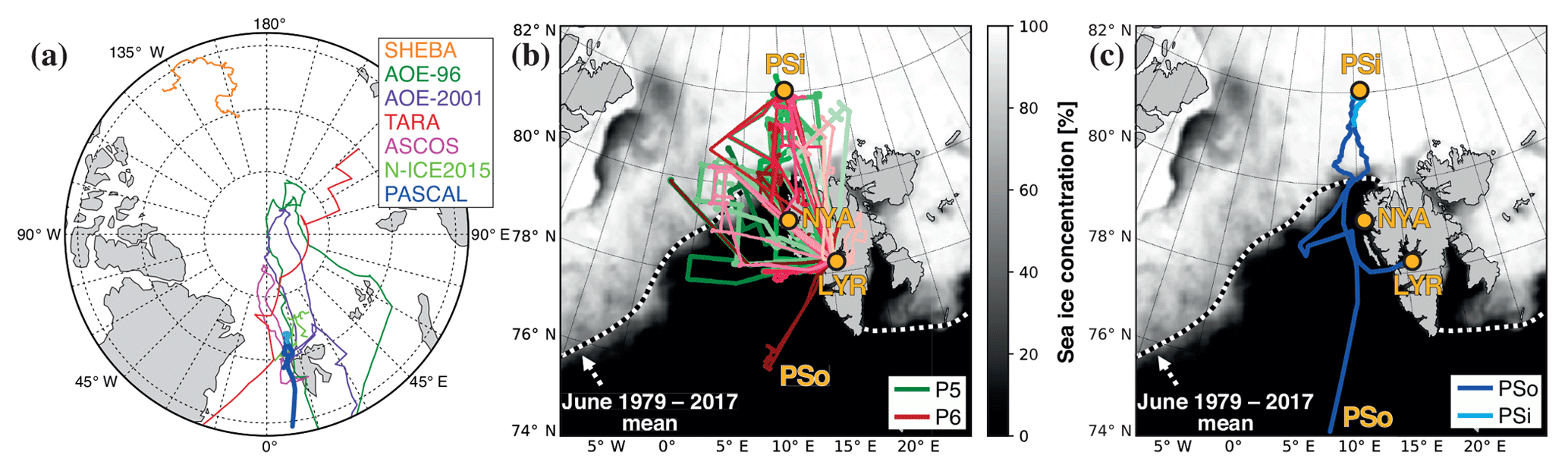
Figure 1Overview of the (a) Arctic and (b, c) ACLOUD/PASCAL region. (a) Tracks of the icebreaker Polarstern during PASCAL (blue) and previous Arctic ship-based campaigns (orange to light green; see Sect. 5.4 for description). For the former, dark and bright colors indicate ocean-cruising (PSo; 30 May–5 June and 17–18 June 2017) and ice-attached (PSi; 6–16 June 2017) positions, respectively. (b) Tracks of the aircraft Polar 5 (green) and Polar 6 (red) flights during ACLOUD (23 May–26 June 2017), with later dates in brighter colors. (c) Track of PSo cruise and PSi position (blue). In panels (b) and (c), codes represent Longyearbyen (LYR), Ny-Ålesund (NYA), PSo entering the ACLOUD/PASCAL region, and PSi, while the shading and the dashed line represent the average sea ice concentration over the ACLOUD/PASCAL measurement period (23 May–26 June 2017) and edge (defined by 15 % concentration) (June 1979–2017), respectively (see Sect. 2.3 for data explanation).
Figure 1b and c illustrate that the climatological mean location of the MIZ runs southwest from Svalbard toward Greenland. During ACLOUD/PASCAL, it extended anomalously close to Svalbard in the near west, north, and east vicinities compared to recent years (Fetterer et al., 2018; Tetzlaff et al., 2014). Therefore, Polarstern was able to moor onto an ice floe relatively close to Svalbard (around 82∘ N, 10∘ E; Fig. 1c), making it easy to reach the icebreaker with Polar 5 and Polar 6 based in Longyearbyen (Fig. 1b). The area of flight activities of ACLOUD extended to Ny-Ålesund and the MIZ west of Svalbard, which were in reach of the aircraft. Within this area, five flights with Polar 5 and Polar 6 were coordinated with A-Train satellite constellation overpasses to characterize the vertical structure of clouds (Stephens et al., 2002).
2.2 Surface-based measurements
Near-surface meteorological and radiosonde data were collected throughout ACLOUD/PASCAL in Ny-Ålesund, at the ice floe station, and aboard Polarstern. The former cover the entire ACLOUD flight period (23 May–26 June 2017), whereas the latter stem from the time when Polarstern was north of the Arctic Circle only (28 May–18 June 2017). These are presented in Sect. 3.1, 3.2, and 4.1.
The AWIPEV research base in Ny-Ålesund is located about 100 km northwest of Longyearbyen. Since 1992, AWI has routinely operated a variety of atmospheric measurements in Ny-Ålesund, which were intensified during ACLOUD/PASCAL. The frequency of the daily radiosonde measurements was increased to four Vaisala RS41 launches per day, providing 6-hourly vertical profiles of temperature, humidity, pressure, and wind speed and direction with about 5 m vertical resolution (Maturilli, 2017a, b). By integration, 6-hourly integrated water vapor (IWV) is retrieved. Standard atmospheric parameters were observed every minute at the surface (Maturilli et al., 2013), of which surface pressure and 2 m temperature are presented here.
In immediate vicinity of the AWIPEV research base, the surface radiation measurements of the Baseline Surface Radiation Network (BSRN) provide information on global and reflective solar radiation (Maturilli et al., 2015). The daily precipitation amount is obtained from the Norwegian Meteorological Institute (MET Norway). Additionally, specific ground-based remote sensing campaign activities to characterize aerosol particles and clouds were conducted by lidar, radar, microwave radiometer, and other instrumentation, as described by Wendisch et al. (2018).
Four daily Vaisala RS92 radiosondes were launched from Polarstern during most of the ACLOUD/PASCAL period (Schmithüsen, 2017). These retrieved vertical profiles are compared to the Ny-Ålesund data, as are pressure observations every minute at 16 m height and temperature observations at 29 m height aboard Polarstern (Schmithüsen, 2018). Detailed information of the instrumentation of Polarstern during PASCAL is summarized by Macke and Flores (2018) and Wendisch et al. (2018).
2.3 Satellites
Polar-orbiting satellites play a key role for studies of sea ice, snow, and cloud variability on a regional scale in the Arctic. Sea ice data for the ACLOUD/PASCAL region in Fig. 1b and c and Sect. 4.3 are obtained from the University of Bremen (UB; Spreen et al., 2017, following Spreen et al., 2008), the National Snow and Ice Data Center (Fetterer et al., 2018), and the Ocean and Sea Ice Satellite Application Facility (Lavergne et al., 2010). They provide sea ice concentration over the ACLOUD/PASCAL measurement period, over the climatological period (1979–2017), and sea ice drift over the ACLOUD/PASCAL measurement period, respectively.
Daily sea ice concentration from UB and NSIDC were obtained at 6 km×4 km and 25 km×25 km resolutions, respectively. The former uses the Advanced Microwave Scanning Radiometer for the Earth Observing System (AMSR-E) and 2 (AMSR2) sensors (Spreen et al., 2017), while the latter is based on observations of the Scanning Multichannel Microwave Radiometer (SMMR), Seasat, Special Sensor Microwave Imager (SSM/I), and Special Sensor Microwave Imager/Sounder (SSMIS) sensors (Fetterer et al., 2018). The multisensory products (AMSR2 and scatterometers) are combined using an advanced cross-correlation method (continuous MCC) for the bidaily sea ice drift data, which were downloaded at a 62.5 km×62.5 km resolution.
The spatially varying date of snowmelt onset in the ACLOUD/PASCAL region relative to climatology is shown in Sect. 5.2. This analysis was based on the method by Markus et al. (2009) (and updated by J. A. Miller of the National Aeronautics and Space Administration Goddard Space Flight Center; NASA GSFC), who used the NSIDC data to develop an Arctic melt season climatology starting in 1979. The method utilizes the agreement of different brightness temperature criteria. Compared to other methods (e.g., buoy data), satellite passive microwave measurements have a larger spatial coverage, have a relative long and consistent record, and are directly related to the melt signature of sea ice or the overlying snow cover. This signature largely fluctuates with snow and ice wetness, which drastically change the dielectric properties of snow and ice and therefore their emissivities.
Cloud properties are routinely retrieved from different polar-orbiting satellite instruments. Unfortunately, considering the special focus on clouds during ACLOUD/PASCAL, the most relevant satellite in the A-train constellation – CloudSat – entered standby mode 4 June 2017 (CloudSat DPC, 2017). Therefore, in Sect. 4.4, we show cloud observations made with the less advanced Infrared Atmospheric Sounding Interferometer (IASI), which is limited in vertical resolution but shows much better spatiotemporal coverage (EUMETSAT, 2017). Infrared sounders are particularly advantageous to retrieve upper-tropospheric cloud properties, with a reliable cirrus identification, day and night (Stubenrauch et al., 2017).
IASI is part of the MetOp series of polar orbiting satellites and has a swath width of about 2200 km (EUMETSAT, 2017). Due to the meridional convergence of the orbits, the temporal sampling of the ACLOUD/PASCAL region is high, with several overpasses per day. Here, we use cloud cover fraction and cloud-top pressure products (level 2, version 6) retrieved from IASI radiance measurements to investigate the distribution of clouds. Cloud detection is performed followed by a retrieval of cloud-top pressure using the CO2-slicing technique for each IASI field of view (Lavanant et al., 2011). As shown by Lavanant et al. (2011), the retrieval of cloud-top pressure works best for homogeneous, opaque clouds common for Arctic regions and is difficult in broken and multi-layer cloud situations.
2.4 Models
Because in situ and satellite data can only provide a limited perspective, reanalysis and operational analysis data from the European Centre for Medium-Range Weather Forecasts (ECMWF) are used to best describe the state of the atmosphere over the broader domain and longer timescales. As one of the objectives of ACLOUD/PASCAL is to investigate the skills of forecast models, explicitly no forecasts are analyzed in this paper.
The European interim reanalysis (Dee et al., 2011) provided data of atmospheric circulation, temperature, and humidity for the ACLOUD/PASCAL region. This reanalysis provides the best description of the state of the atmosphere by assimilating a wealth of observations, including satellites, radiosondes (also the ones described in Sect. 2.2 from Ny-Ålesund and Polarstern), and land stations, and is found to be well suited for the northern regions (Chung et al., 2013; Jakobson et al., 2012; Lindsay et al., 2014).
ERA-I data were acquired on a horizontal grid for the period of May–June 1979–2017. These data served as the basis for the identification of atmospheric rivers affecting Ny-Ålesund discussed in Sect. 3.1, following the algorithm by Gorodetskaya et al. (2014) and adapted for the Arctic. In the calculation of the weather events in Sects. 3.3 and 5.3, 6-hourly 850 hPa and skin temperature and 850 hPa geopotential were used. Parameters presented in Sect. 4.2 are based on 6-hourly 700 hPa geopotential, zonal and meridional winds, temperature, and specific humidity. The 700 hPa virtual potential temperature is estimated from the last two and is therefore a merged measure of air temperature and humidity (Etling, 2008). Daily 1000 hPa geopotential was obtained for Sect. 5.1.
ECMWF operational analysis data were obtained on a horizontal grid. These were used for the synoptic description in Sect. 3.1 and provided the input for the Lagrangian FLEXible PARTicle dispersion model (Stohl et al., 2005) used to analyze the history of air masses arriving in Ny-Ålesund in Sect. 4.1.
Using FLEXPART, we continuously released 480 000 individual air parcels close to the surface at the location of Ny-Ålesund for every day of the campaign period. These air parcels represent an inert air mass tracer and were further traced back in time for another 10 days. The distribution of this air mass tracer – and thus the pathway of the trajectories through the atmosphere – does not only depend on the mean wind given in the operational analysis data but also on turbulent motions (Stohl et al., 2005). These motions also affect the center of mass trajectories, contrasting the commonly used kinematic trajectories that only depend on the mean wind field from meteorological input data. Using this amount of individual air parcels and considering the turbulent motions allow us to obtain a better estimate of the distribution of the air masses, which potentially affected the observations in Ny-Ålesund.
In backward mode, FLEXPART provides potential emission sensitivity (PES), which is the response function of the source–receptor matrix (Seibert and Frank, 2004). PES is directly related to the residence time of a particle in a model grid box and measures the simulated concentration at the receptor that a source of a unit strength in this model box would produce for an inert tracer not affected by any removal process (Hirdman et al., 2010; Stohl et al., 2005). We used PES available on a 0.25∘ grid in the horizontal, which represents the entire tropospheric column.
In this section, time series from Ny-Ålesund and Polarstern over the course of the ACLOUD/PASCAL measurement period are analyzed to characterize the temporal evolution of the atmospheric state. These are meteorological parameters from near-surface and radiosonde observations in Sect. 3.1 and 3.2, respectively. Time series of weather classifications based on reanalysis data follow in Sect. 3.3. A more detailed description of the day-to-day weather development as observed by Polarstern is reported by Macke and Flores (2018).
3.1 Near-surface meteorological observations
Figure 2 shows time series of key meteorological parameters from Ny-Ålesund and Polarstern during the ACLOUD flight period and PASCAL ocean-cruising and ice-attached periods, respectively. The permanent observations from AWIPEV and MET Norway weather stations allow a comparison of the ACLOUD/PASCAL period to the observed long-term average (1993–2016). To illustrate the synoptic situation, weather charts are provided for key days in Fig. 3, showing maps of surface pressure and 500 hPa geopotential height.
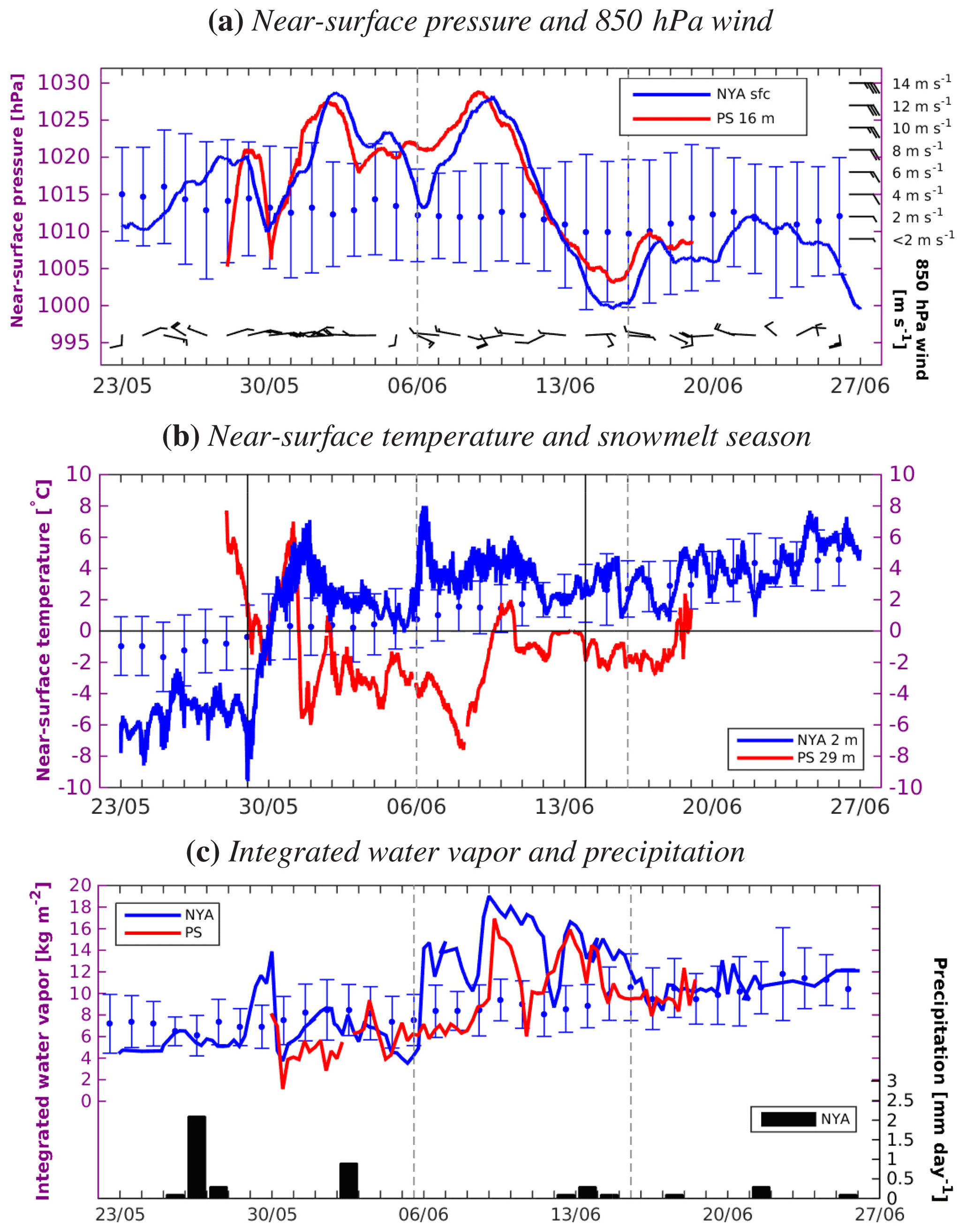
Figure 2(a) Near-surface pressure (graphs) and 850 hPa horizontal wind (bars for speed, vectors for direction), (b) near-surface air temperature (graphs) and snowmelt season (solid vertical lines), and (c) vertically integrated water vapor (graphs) and precipitation (bars) measured at Ny-Ålesund (NYA; blue and black) and Polarstern (PS; red) over the ACLOUD/PASCAL measurement period (23 May–26 June 2017). Dots and intervals indicate daily average and standard deviation, respectively, over the Ny-Ålesund long-term period (1993–2016). Dashed vertical lines distinguish the Polarstern ocean-crossing periods from the ice-attached period (6–16 June).
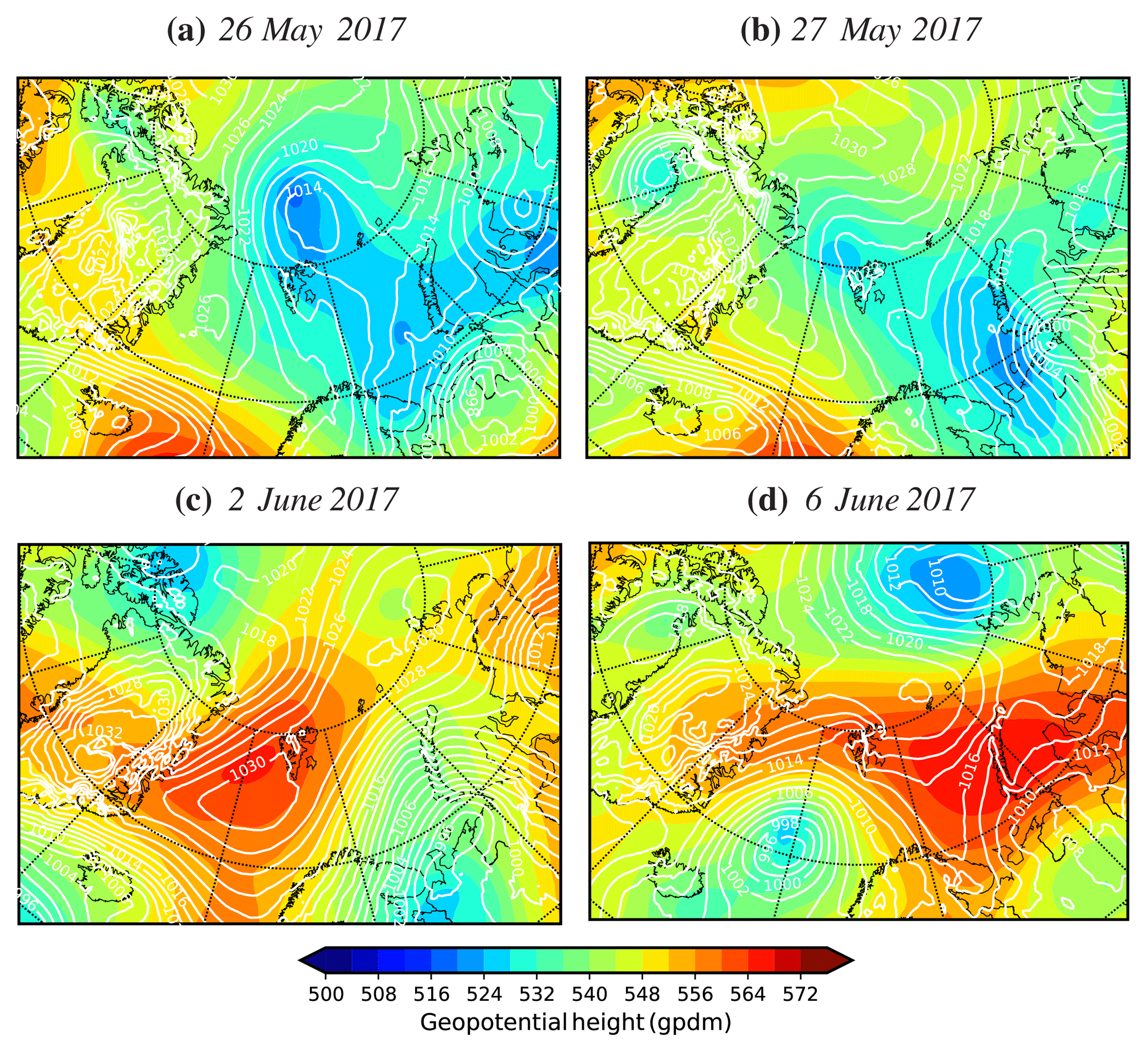
Figure 3Sea level pressure (in hPa; white contours) and 500 hPa geopotential height (in meters; shading) for 12:00 UTC on (a) 26 May, (b) 27 May, (c) 2 June, and (d) 6 June 2017, from ECMWF.
As observed in Ny-Ålesund, the ACLOUD flight period started in a cold and dry period during northerly winds (Fig. 2). This situation was caused by low pressure systems east and north of Svalbard and a high pressure system over Greenland on 26 May (Fig. 3a). In this region, such pressure patterns are typical when marine cold air outbreaks (Kolstad, 2017) are forming with strong off-ice flow over the Fram Strait, which is indicated by the isobars oriented parallel to the west coast of Svalbard.
After about 3 days, this pressure pattern started to change, which finally led to the onset of melting (explained below). The first indication of this change was a pressure increase in Ny-Ålesund and more variable wind direction (Fig. 2a). This variability was caused by the changing position of the above-mentioned low pressure system northeast of Svalbard (Fig. 3a), first moving toward the northwestern edge of the archipelago (not shown) and then southward along its western coast on 27 May (Fig. 3b). In Ny-Ålesund, the cyclonic rotation of this low pressure system gave westerly winds and an advection of humid air (Fig. 2a and c). This development caused the highest precipitation during ACLOUD/PASCAL, with 2 mm liquid equivalent of snowfall on 27 May (Fig. 2c).
The following days saw IWV and temperature substantially increase in Ny-Ålesund, from 6 kg m−2 on 28 May to 14 kg m−2 on 30 May (Fig. 2c) and from −10 ∘C on 29 May to+7 ∘C on 31 May (Fig. 2b), respectively. The former increase was related to a narrow band of high IWV and intense integrated water vapor transport (IVT), identified as an atmospheric river, which reached Svalbard from western Siberia on 30 May (Fig. A1a). In this period, precipitation occurred in the ACLOUD/PASCAL region but was confined to a small area. After this event, the wind direction turned northerly again due to a strong low that formed southeast of Svalbard (not shown), advecting more cold air from the ice-covered areas.
Then, 3 days later, a strong southwesterly flow developed due to a high pressure system over the Greenland Sea (Fig. 3c), advecting warm air from lower latitudes. This triggered the melt onset over the northern Fram Strait. This development explains the increasing surface pressure up to 1029 hPa observed in Ny-Ålesund on 2 June (Fig. 2a). Coincidentally, a low pressure system developed over northern Greenland. These two pressure systems north and south of Svalbard led to strong southwesterly air advection across the northern Fram Strait. On the northerly cruising Polarstern in the waters west of Spitsbergen (Fig. 1c), temperatures rose from −2 ∘C on 29 May to +7 ∘C on 31 May (Fig. 2b). This short period was the only time that the temperature records of Ny-Ålesund and Polarstern perfectly matched. With Polarstern being south (north) of Ny-Ålesund until 30 May (from 31 May), the meridional temperature gradient caused significant differences between the two time series. Similarly, the rapid cooling observed on Polarstern from +7 to −6 ∘C over 31 May coincided with its entrance into the sea ice northwest of Spitsbergen (Fig. 1c).
The 17 ∘C warming within only 2 days in Ny-Ålesund, which marked the beginning of the snowmelt season on 29 May (Fig. 2b), was also imprinted in the time series of snow albedo obtained by the surface radiation measurements. From this date, the surface albedo temporarily decreased from 0.9 to lower values, before it rapidly dropped to below 0.1 by 14 June, when the snow had completely disappeared. This development agrees with the climatology of Ny-Ålesund, which reports the first snow-free day between 30 May and 5 July since the beginning of the BSRN measurements in late 1992.
The period of warm temperatures at the beginning of June represent the highest positive temperature anomaly recorded during ACLOUD/PASCAL. In Ny-Ålesund, 7 and 8 ∘C were observed on 31 May and 6 June, respectively (Fig. 2b), both being indications of warm air advection (Tjernström et al., 2015). The latter event was accompanied by an increase of IWV to 15 kg m−2 (Fig. 2c), which was linked to another atmospheric river episode reaching Ny-Ålesund from the east (Fig. A1b).
6 June was also the date when the observations from the ice-attached Polarstern started. Over its first days in the ice, the sea ice camp observed an increase in near-surface pressure due to a high pressure ridge east of Svalbard (Fig. 3d), reaching a maximum of 1029 hPa on 8 June. IWV rose from 6 to 17 kg m−2 on 9 June (Fig. 2c) and near-surface air temperature from −8 to +2 ∘C on 10 June (Fig. 2b). In other words, the above-freezing temperature on Polarstern while surrounded by sea ice (1–17 June) occurred 4 days after that in Ny-Ålesund, which is later than that arising from the pure air mass transport. This delay can be explained by the more northerly location of Polarstern within the compact sea ice, where surface cooling fosters a stable inversion layer close to the ground, while warm air advection occurs in the free troposphere above. As long as the inversion is not destroyed, it remains cold at the lowest levels. Anomalously warm and moist air was also observed in Ny-Ålesund on these days but with less intense changes due to the already warm and moist air starting on 6 June. Thus, while the synoptic conditions were similar for Ny-Ålesund and Polarstern during 6–8 June (Fig. 2), local factors (e.g., sea ice distribution) probably played an important role for the difference between the two stations at about 335 km apart.
Both Ny-Ålesund and Polarstern experienced distinct drops in near-surface pressure associated with increases of near-surface air temperature and IWV around 13 June (Fig. 2a to c). The air mass reaching the ACLOUD/PASCAL region on this day had a European origin but circled once around Svalbard before arriving Ny-Ålesund from the north (shown later in Fig. 7c). The peaks in the IWV observed in Ny-Ålesund on 9 and 13 June can be explained by air masses with high IWV but no intense IVT on those days (Fig. A1c and d). For the remainder of the measurement period, surface pressure, near-surface air temperature, and IWV observed in Ny-Ålesund were close to the long-term average, as well as close to Polarstern values until the icebreaker left the ice (18 June).
With the exceptions described above, Ny-Ålesund and Polarstern observations presented in Fig. 2 are comparable. This indicates that both locations mostly were influenced by the same synoptic systems. The same conclusion was obtained for observations of the N-ICE2015 experiments, when measurements from Ny-Ålesund and a research vessel north of Svalbard were compared (Kayser et al., 2017). It is, therefore, appropriate to set the observations of the ACLOUD/PASCAL measurement period into context with the long-term observational record from Ny-Ålesund.
In contrast to the N-ICE2015 expedition (Cohen et al., 2017), no prominent cyclones were observed during the ACLOUD/PASCAL campaign. Only on 28 June (indicated by the negative tendency in surface pressure in Ny-Ålesund on 27 June in Fig. 2a), a cyclone passed the region and prevented any flight activities. Hence, analysis of synoptic-scale dynamics related to cyclones similar to, for example, Knudsen et al. (2015), Akperov et al. (2018), or Zahn et al. (2018), is not needed in this paper.
3.2 Radiosonde observations
To investigate the coupling of the surface, the boundary layer, and the free troposphere, time series of temperature and specific humidity profiles from Ny-Ålesund and Polarstern are shown in Figs. 4 and 5 for the ACLOUD/PASCAL measurement period. Specific humidity in Figs. 4b, d, and 5b was calculated using the vapor pressure formulations by Hyland and Wexler (1983). ABL heights in Figs. 4 and 5 are identified using the surface-based bulk Richardson number approach assuming a critical value Ri of 0.25, as suggested by Hanna (1969), Zhang et al. (2014), and Kayser et al. (2017). For readability, time series of wind profiles are included in Fig. 4c and d from Polarstern only. However, the time series of 850 hPa wind from Ny-Ålesund is shown in Fig. 2a.
The daily long-term radiosonde records, following Maturilli and Kayser (2017), demonstrate the increase in air temperature and specific humidity from 23 May to 26 June (Fig. 4a and b). By the beginning of June, near-surface air temperature (specific humidity) usually exceeds 0 ∘C (3 g kg−1).
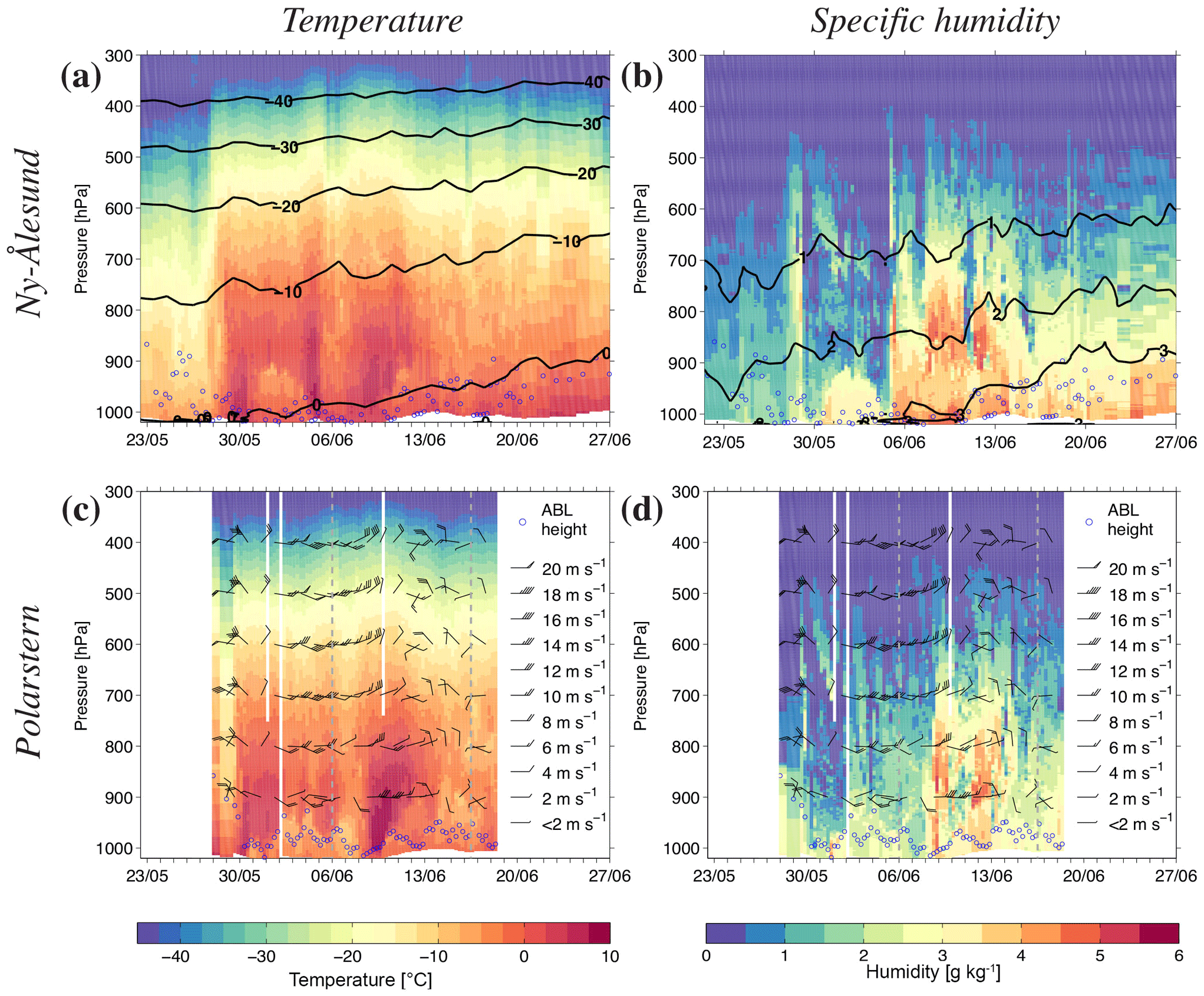
Figure 4Vertical profiles of (a, c) temperature and (b, d) specific humidity measured at (a, b) Ny-Ålesund and (c, d) Polarstern over the ACLOUD/PASCAL measurement period (23 May–26 June 2017). Blue circles indicate the height of the atmospheric boundary layer (ABL). Black contour lines in (a, b) represent the respective 1993–2016 average, while black arrows in (c, d) represent 2017 values of wind speed and direction. Dashed vertical lines in (c, d) distinguish the Polarstern ocean-crossing periods from the ice-attached period (6–16 June).
As indicated by the near-surface air temperature observations in Ny-Ålesund (Fig. 2b), the anomalously cold first week with subfreezing temperatures was followed by two exceptionally warm weeks partially above 5 ∘C (Fig. 4a and c). This rapid change around 30 May obviously occurred throughout the entire tropospheric column.
The WAA starting around 29 May over Ny-Ålesund only shortly enhanced tropospheric humidity levels (Fig. 4b). Over Polarstern, no significant changes in specific humidity were associated with this event and the following period between 31 May and 5 June. Slightly raised values with around 3 g kg−1 were observed only in the lowest 100 hPa (Fig. 4d). This situation changed during a second WAA and first sustaining moist air intrusion on 6 June, when the temperature and humidity in the lowest 300 hPa over Ny-Ålesund (Polarstern) significantly increased and reached values up to +8 ∘C (+4 ∘C) and 5 g kg−1 (4 g kg−1), respectively, for a period of about a week. During this period, the temperature and humidity exceeded the long-term averages with the highest anomaly observed around 8–12 June.
The wind vectors in Fig. 4c and d indicate that the highest temperatures and humidities occurred in association with a shift to generally easterly winds below 700 hPa (southerly below 850 hPa during 7–9 June). Air from the east (south) warmed and moistened over the open ocean west and southwest of Franz Josef Land (Spitsbergen). Above 700 hPa, a northerly wind component dominated.
However, the prevailing winds changed during 11 and 12 June, when northerly winds started to dominate the lower troposphere, indicating the end of the moist air intrusion. Until the end of the measurement period, the temperature and specific humidity over Ny-Ålesund remained close to the long-term averages.
The radiosondes, given their high vertical resolution, further allow the investigation of temperature and humidity inversion variabilities during the ACLOUD/PASCAL period. Inversions are a dominant feature of the Arctic wintertime boundary layer. In spring, the frequency of inversions decreases but still significantly impacts the atmospheric temperature, moisture, and energy exchange. Temperature inversions have significant impacts on the atmospheric stratification (Lesins et al., 2010) and manipulate the vertical distribution of longwave radiation (Bintanja et al., 2011). In particular, specific humidity inversions are known to be a source of longwave radiative heating of the surface during cloud-free conditions (Devasthale et al., 2011) and are relevant for cloud physics (Sedlar et al., 2012; Solomon et al., 2011). For these reasons, Fig. 5 provides a more detailed picture of the boundary layer processes during ACLOUD/PASCAL, showing the retrieved altitudes of surface-based and lifted inversions observed in the radio soundings over Polarstern. The inversions were identified following the methods described in Andreas et al. (2000), Kahl (1990), and Kayser et al. (2017).
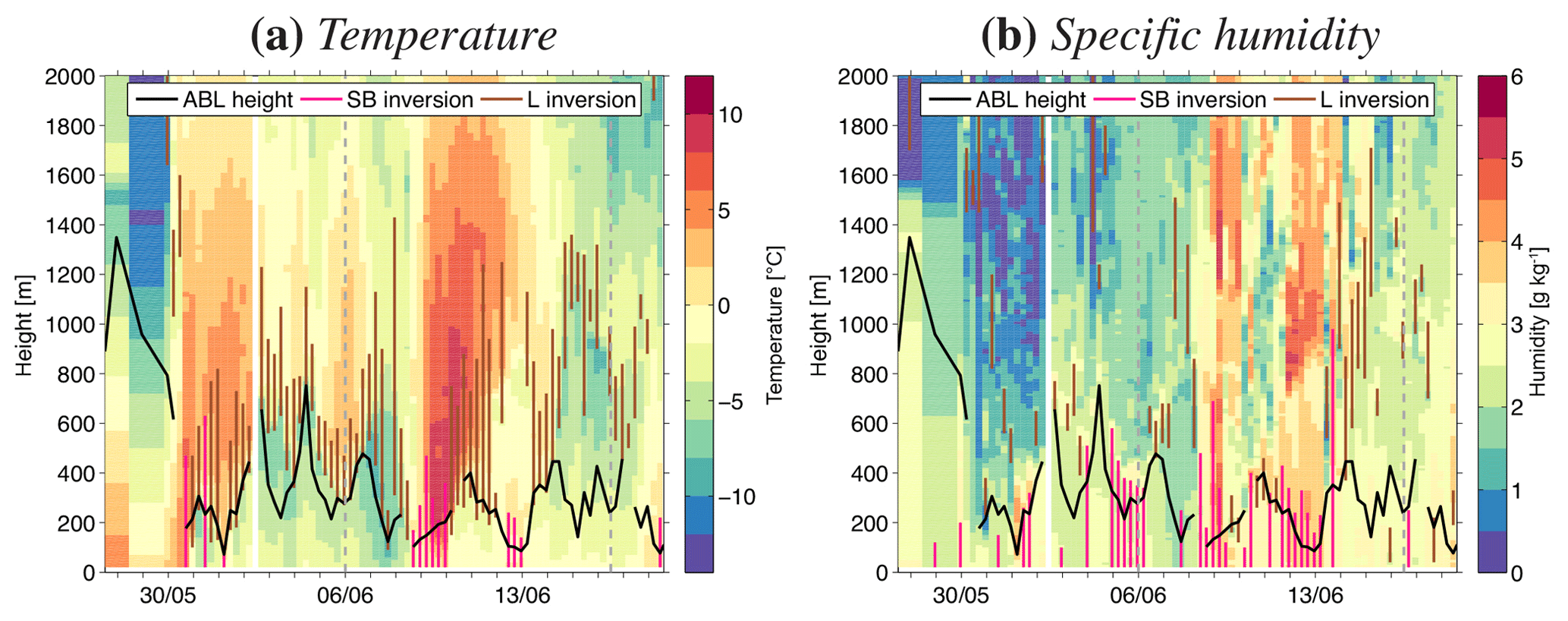
Figure 5Vertical profiles of (a) temperature and (b) specific humidity measured at Polarstern over the PASCAL measurement period (28 May–18 June 2017). Pink and brown vertical lines indicate the vertical extent of the lowermost surface-based (SB) and lifted (L) inversions, respectively, while black contour lines indicate the atmospheric boundary layer (ABL) height corresponding to the blue circles in Fig. 4. Dashed vertical lines distinguish the Polarstern ocean-crossing periods from the ice-attached period (6–16 June).
During the ACLOUD/PASCAL measurement period, inversions were found in most soundings for both temperature and specific humidity, particularly throughout June when Polarstern was located in areas covered by sea ice. During the period of the ice floe camp (6–16 June), an enhanced occurrence of surface-based inversions was found. This was caused by temperature and humidity advection above the boundary layer, while the ice surface remained at a temperature of 0 ∘C, stabilized by the snowmelt. In general, a lifted temperature inversion was present when the ABL was relatively high (up to 700 m), while a surface-based temperature inversion was observed when the ABL was shallow (about 200 m).
3.3 Weather classification
As shown by the observed time series, the weather during ACLOUD/PASCAL was influenced by different synoptic atmospheric patterns. A way to quantify the dominant synoptic pattern is to analyze the occurrences of MCAOs. Following Papritz et al. (2015) and Kolstad (2017), the MCAO index is defined as the difference between surface and 850 hPa potential temperature of each grid point, area averaged over the eastern Greenland Sea (here defined as 75.00–80.25∘ N, 4.50–10.50∘ E). Land grid cells and cells for which the surface temperature is lower than 271.5 K are excluded from the area averaging.
Time series of the 6-hourly MCAO index are calculated for the ACLOUD/PASCAL period and used to identify events of cold air outbreaks. A new event begins when the index is greater than 0 K and ends if the index falls below 0 K. Then, the last time for which the MCAO index is >0 K is set as the final time step of the event. Events are recorded only if an index value of at least 2 K is reached and the duration is at least 48 h. The maximum MCAO index of each event is required to occur within the ACLOUD/PASCAL measurement period, but the events are allowed to start any time in May or by the end of June. The threshold of 2 K is lower than that in studies focusing on the cold season (e.g., 3 K in Kolstad, 2017). The lowered threshold accounts for the fact that MCAOs are considerably less frequent and are considerably less severe in early summer than in winter (Fletcher et al., 2016).
The MCAO index time series also indicate the occurrence of WAA. While MCAOs are characterized by a change of atmospheric stratification toward stable conditions, i.e., positive values of the MCAO index, WAA is identified by a strongly negative deviation of the MCAO index relative to the climatology. For the identification of a WAA event, here we used a threshold of −10 K in the difference between the actual MCAO index and the average over 1979–2016, before the procedure follows that for the MCAO events.
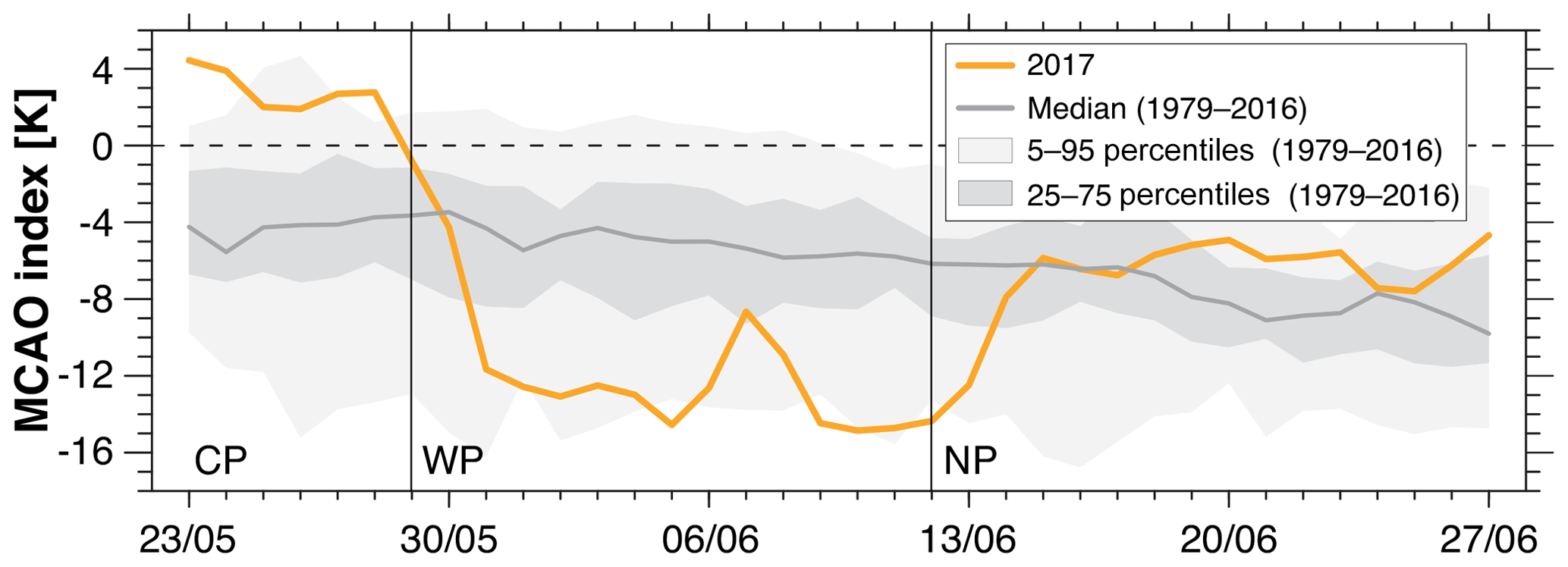
Figure 6Marine cold air outbreak (MCAO) index for the eastern Greenland Sea (75.00–80.25∘ N, 4.50–10.50∘ E) over the ACLOUD/PASCAL measurement period (23 May–26 June 2017), based on ERA-I data. The gray median line and percentile shading refer to the climatology over 1979–2016, while the black vertical lines separate the three key periods (CP, WP, and NP) in 2017 defined in Sect. 4.
As shown in Fig. 6, the MCAO index varied considerably over the first 3 weeks of ACLOUD/PASCAL. During the first 8 days (23–30 May), values were above the median of the climatology and mostly exceeded the 95th percentile until 28 May. Corresponding to the anomalously cold and dry air observed in Figs. 2 and 4, we identify a MCAO event during the first week of the measurement period (maximum 23 May in Fig. 6). The MCAO index then dropped significantly from +2 K on 28 May to −11 K on 31 May, remaining below the median until 15 June. During these 2 weeks, values remained below −12 K (i.e., below the 25th percentile) except for 7 June. In combination with the temperature and humidity time series (Figs. 2 and 4), we identify two WAA events during the second and third weeks of the measurement period (minima on 5 and 10 June in Fig. 6). After 14 June, the MCAO index increased again and leveled around the long-term median between −5 and −7 K, indicating normal weakly unstable conditions in the lower troposphere (i.e., neither MCAO nor WAA conditions).
The MCAO index arguably offers a better understanding of the local weather as compared to the large-scale Arctic oscillation and dipole indices. These are shown for comparison in Fig. A2 in the Appendix and will be discussed more in a climatological context in Sect. 5.1.
In this section, we highlight the characteristics of three key periods, as defined based on the time series shown in Sect. 3. These serve as the basis for the regional and local meteorological data shown for each of the key periods in Sect. 4.1, 4.2, 4.3, and 4.4.
Based on Figs. 2–6 (and discussions thereof in Sect. 3.1–3.3), we define the following key periods during the ACLOUD/PASCAL measurement period:
-
the cold period (CP) – 23–29 May 2017 (7 days),
-
the warm period (WP) – 30 May–12 June 2017 (14 days), and
-
the normal period (NP) – 13–26 June 2017 (14 days).
The three key periods represent three different synoptic tendencies and not states. For example, CP ends as the near-surface air temperature in Ny-Ålesund starts rising (on 29 May) and not when it exceeds 1 standard deviation (on 31 May) (Figs. 2b and 4a).
4.1 Air mass distribution
To assess differences in the air mass histories of the three key periods defined above, we compare their mean trajectories. This analysis was performed using FLEXPART in backward mode, with input data from ECMWF operational analysis (see Sect. 2.4). In addition to the temporal means of PES over each key period, Fig. 7 also shows the daily center of mass trajectories of the respective key period.
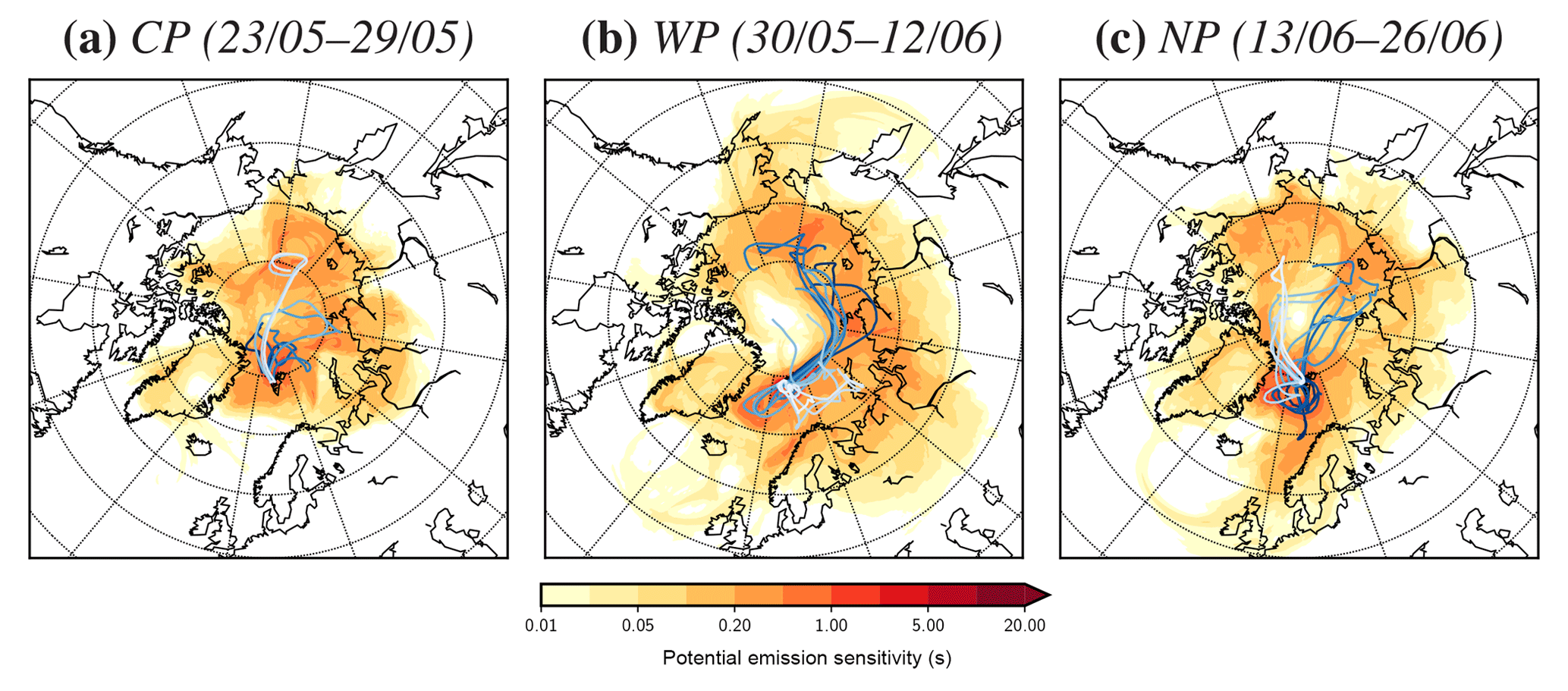
Figure 7Ranges of continuous daily potential emission sensitivities (shading) and daily center of mass backward trajectories to Ny-Ålesund, with later masses in brighter colors (trajectories) for each ACLOUD/PASCAL key period from FLEXPART. The key periods are defined as (a) the cold period (CP), (b) the warm period (WP), and (c) the normal period (NP).
During CP, most air masses reaching Ny-Ålesund originated from within 70∘ N without significant midlatitude influence (Fig. 7a). Their origin was mostly the central and eastern parts of the Arctic Ocean, with smaller contributions from the Siberian coast, the Canadian Arctic, and Greenland. This Arctic air was cold and dry, as indicated in Figs. 2b, c, and 4a, b.
In the twice-as-long WP, the trajectories spanned a larger area, originating as far south as 50∘ N (Fig. 7b). Three major areas then influenced the air mass characteristics reaching Ny-Ålesund: northern Europe, Siberia, and the Arctic North Pacific sector. There was only a weak influence from the North American archipelago and the central Arctic Ocean.
During the first WP week, the air parcels entered the Nordic Seas from the eastern Arctic Ocean, either crossing over Svalbard from the east or going around the archipelago to arrive in Ny-Ålesund from the southwest. These two pathways are expected to warm the air masses adiabatically across Spitsbergen or thermodynamically over the ocean, respectively (cf. discussion in Sect. 3.1). These two patterns are imprinted in the temperature and humidity time series shown in Fig. 4a and b, where the latter pattern is also characterized by higher humidity from the ocean. While originating in the Nordic Seas or over northwestern Eurasia, air masses during the second WP week also crossed open water before reaching Ny-Ålesund from the south, thus being similar to the latter of the two described patterns.
The PES distribution of the last key period – NP – was a mixture of the two former key periods. Most of the Arctic Ocean and the Nordic Seas were then sources of air mass origin, but the highest density was found in air arriving Ny-Ålesund from the west (Fig. 7c). The relatively average temperate and humid air observed here (Figs. 2b, c, and 4a, b) can potentially result from the air masses passing over the sea ice north of Greenland, the open ocean south of Svalbard, or the Greenland ice sheet. These air masses could be heated either by adiabatic motions or through sensible or latent heat fluxes from the ocean into the atmosphere during their transport from the sea ice/open ocean transition zone in the Fram Strait to Ny-Ålesund.
Figure 8 shows the varying profiles of temperature and specific humidity as observed over Ny-Ålesund and Polarstern during the three key periods. Only Ny-Ålesund data are included in Fig. 8a and b due to the southerly location of Polarstern during the first campaign week, unrepresentative of the Arctic. In Fig. 8c–f, Polarstern data are split into two profiles to differentiate its ice-attached and ocean-cruising locations (see Fig. 1c).
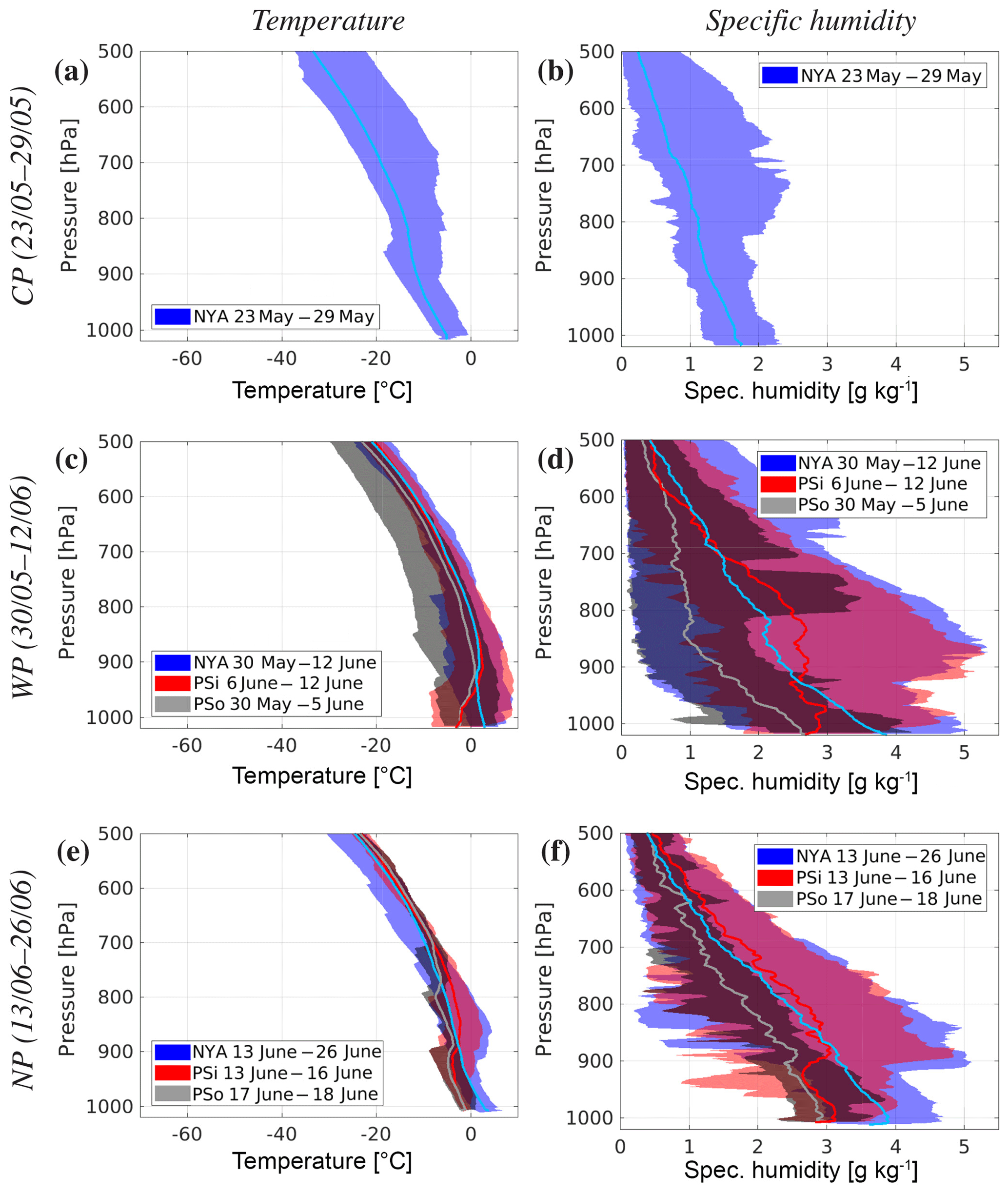
Figure 8Average (graphs) and minimum-to-maximum range (shading) vertical profiles of (a, c, e) temperature and (b, d, f) specific humidity for each ACLOUD/PASCAL key period from Ny-Ålesund (blue) and Polarstern (red for ice-attached dates, gray for cruising dates). Key periods are defined as (a, b) the cold period (CP), (c, d) the warm period (WP), and (e, f) the normal period (NP).
The first key period (CP) was characterized by relatively cold and dry air above Ny-Ålesund, with temperatures continuously below 0 ∘C and humidity mostly below 2 g kg−1 (Fig. 8a and b). The nearly isothermal average profile between 900 and 800 hPa is consistent with the top of the frequent low-level clouds observed during this period (shown later in Fig. 11b). No inversions prevail in the average temperature and humidity profiles, although some individual soundings show humidity inversions around 820 hPa, where the radiosondes escape the mountain ridges and enter the synoptic flow.
During the second key period (WP), two features were noteworthy. Firstly, above Ny-Ålesund, a rather weak temperature inversion (< 1 ∘C) was detected in the average profile at 910 hPa, while the lower troposphere had warmed (+10 ∘C) and moistened (+5 g kg−1) substantially with respect to CP (Fig. 8c and d compared to Fig. 8a and b). Secondly, during WP above Polarstern, a marked temperature inversion of about 5 ∘C prevailed in the lowest 100 hPa for both ice-attached and ocean-cruising periods. Moreover, elevated humidity inversions of 1.0–1.5 g kg−1 were detected in individual soundings.
During the third key period (NP), the averaged temperature profile above Ny-Ålesund formed a similar shape to that during CP, revealing no inversions but a warming of about 10 ∘C (Fig. 8e) and a moistening of about 2 g kg−1 (Fig. 8f). Above Polarstern, weak temperature inversions were present in the average profiles. Individual soundings with an elevated humidity inversion appeared at 900 hPa above both Ny-Ålesund and the ice-attached Polarstern. This feature was not seen above the ocean-cruising Polarstern, possibly due to the few soundings in this profile (2 days only).
4.2 Atmospheric circulation and thermodynamics
Figure 9 complements Figs. 7 and 8 by picturing the contrasting atmospheric circulation, temperature, and humidity of the three key periods based on ERA-I data. Here, Fig. 9a, c, and e illustrate the 700 hPa geopotential height and horizontal wind of CP, WP, and NP, respectively, while the relative temperature and humidity of these periods are depicted in Fig. 9b, d, and f. In addition to their climatology, each panel depicts the anomalous conditions of the three key periods compared to their respective climatology. A more detailed evolution of the atmospheric circulation and thermodynamics observed during ACLOUD/PASCAL is presented by daily fields of these measures in Videos S1 and S2 in the Supplement. The 700 hPa level represents the main flight level during ACLOUD (Wendisch et al., 2018).
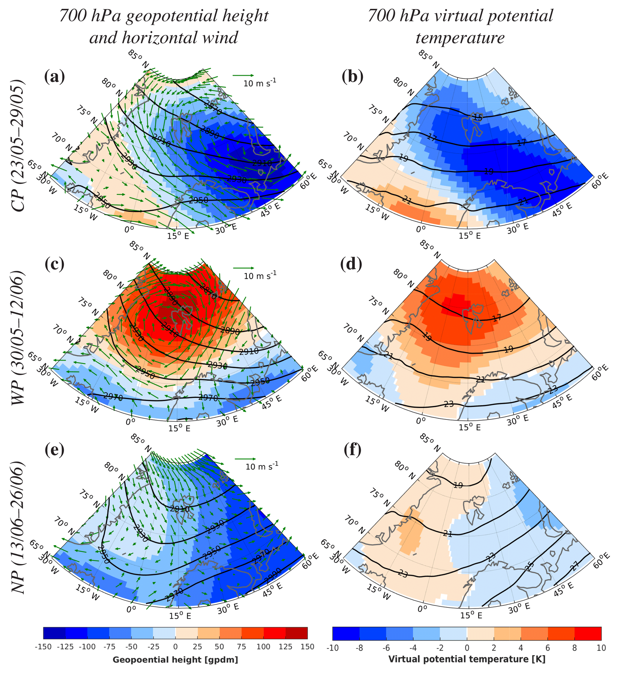
Figure 9Climatologies (1979–2016; contours) and anomalies relative to climatologies (2017 minus 1979–2016; shading) of 700 hPa (a, c, e) geopotential height with key period median horizontal wind (vectors) and (b, d, f) virtual potential temperature for each ACLOUD/PASCAL key period based on ERA-I data. Key periods are defined as (a, b) the cold period (CP), (c, d) the warm period (WP), and (e, f) the normal period (NP).
Figure 9a and b confirm the synoptic pattern identified for the first campaign week (CP) in Figs. 2, 4, and 7. A northerly airflow west and north of Spitsbergen at 700 hPa follows from the anomalous low geopotential height centered over the Pechora Sea in the southeastern Barents Sea (Fig. 9a). The dry and cold Arctic air decreased the virtual potential temperatures down to −9 ∘C, which is lower than the climatology in the Barents Sea (Fig. 9b). Similarly, temperatures were 4–8 ∘C below the climatology of 13–17 ∘C in the ACLOUD/PASCAL region.
There was a prominent change in atmospheric circulation during the next 2 weeks of ACLOUD/PASCAL (WP; Fig. 9c compared to Fig. 9a). While the climatology did not change much, the anomalous high 700 hPa geopotential height centered over the Fram Strait, Svalbard, and north of the archipelago caused an anticyclonic wind pattern in the region (Fig. 9c). Moist and warm maritime air was advected from the Norwegian and Greenland seas into the region, with virtual potential temperature values reaching 8 ∘C above the climatology at the ice edge northwest of Spitsbergen (Fig. 9d). Relative to the Cap of the North, which then was in a northeasterly wind regime (Fig. 9c), the ACLOUD/PASCAL region was about 5 ∘C warmer and moister (Fig. 9d).
During the final 2 weeks of ACLOUD/PASCAL (NP), 700 hPa atmospheric circulation resembled that of the first week but without distinct minimum in geopotential height anomalies (Fig. 9e compared to a and c). Instead, the lowest values were generally found from Novaya Zemlya to Franz Josef Land. This meridional anomaly contrasted the climatological trough over the Greenland Sea and caused a northwesterly airflow around Svalbard (Fig. 9e). As a result, 700 hPa virtual potential temperature values were close to the climatology, generally in the range 0–2 ∘C west of 15∘ E (including the ACLOUD/PASCAL region) and −2–0 ∘C east of this meridian (Fig. 9f). While the air came from the Arctic, its northwesterly origin in NP compared to northeasterly in CP allowed adiabatic heating over the Greenland ice sheet (cf. discussion in Sect. 4.1). Furthermore, during NP, the sea ice melted substantially northeast of Greenland (shown later in Fig. 10c). Hence, the relative warm and moist water underneath likely altered the Arctic air above.
4.3 Sea ice dynamics
To answer the question of whether the characteristic key periods also were detectable in sea ice dynamics, the sea ice concentration, edge, and drift are investigated in Fig. 10. Common for all three periods, the position of the sea ice edge did not change much in the Fram Strait. Sea ice concentration was anomalously high in the MIZ west (typically 20 %–30 %), north (typically 40 %–50 %), and east (typically 30 %–40 %), respectively, while anomalously low south (typically 30 %–40 %) of Svalbard (cf. discussion in Sect. 2.1). Even so, there were marked changes in sea ice dynamics throughout ACLOUD/PASCAL.
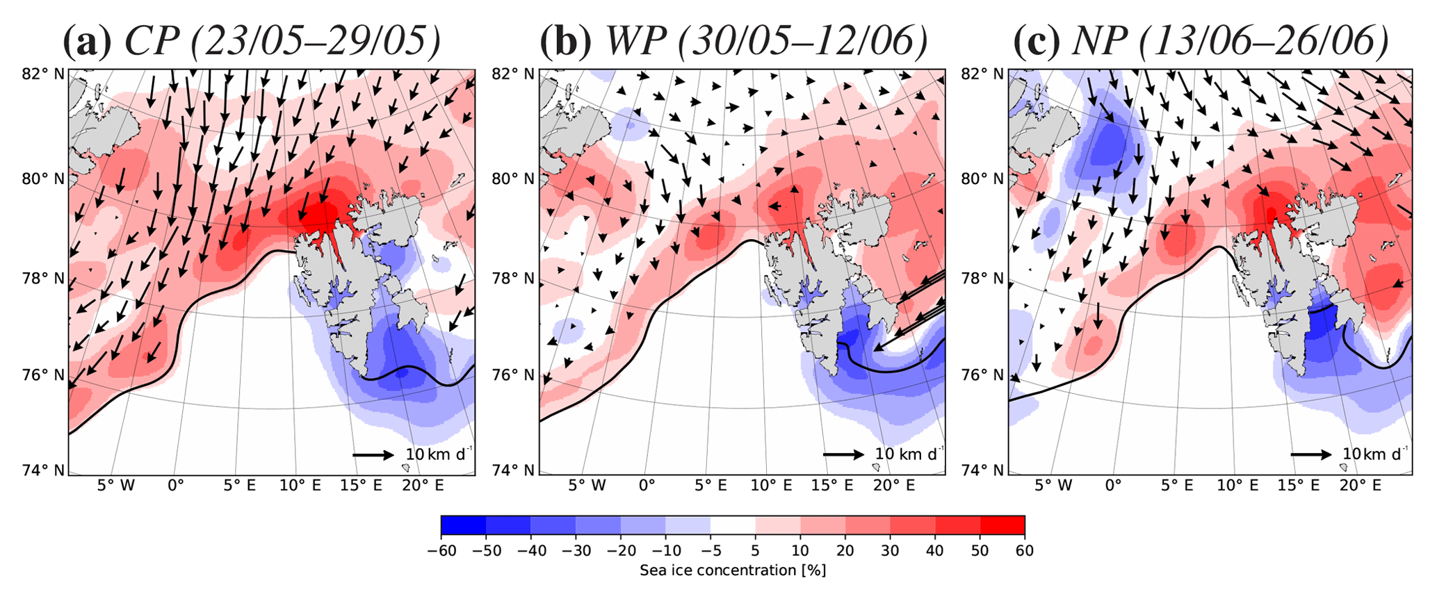
Figure 10Anomalous sea ice concentration relative to climatologies (2017 minus 1979–2016; shading) and average sea ice drift (2017; vectors) for each ACLOUD/PASCAL key period from UB, NSIDC, and OSI SAF. The key periods are defined as (a) the cold period (CP), (b) the warm period (WP), and (c) the normal period (NP). White shading south of the 2017 sea ice edge (line) indicates open water.
During CP, the northerly wind (Fig. 9a) caused a strong southerly to southwesterly sea ice drift of about 10 km day−1 and a positive concentration anomaly in the Fram Strait (Fig. 10a). This was particularly pronounced north of Svalbard, with sea ice concentrations up to 50 % above climatology.
The southerly wind during WP (Fig. 9c) reduced the drift of sea ice out of the Fram Strait (Fig. 10b). Instead, the sea ice compacted, resulting in the narrower band of anomalous high sea ice concentration (5 %–30 % above climatology) near the ice edge north and west of Svalbard.
The band of anomalous high sea ice concentration did not significantly change during NP (Fig. 10c). Then, the northwesterly wind (Fig. 9e) enhanced the ice export into the Barents Sea and contributed to the formation of the Northeast Water Polynya (Fig. 10c). The polynya, described by Pedersen et al. (1993; as cited in Schneider and Budéus, 1997), is a common phenomenon, but in 2017 opened faster and extended further north than usual, as indicated by down to 30 % lower sea ice concentration compared to the climatology off the Greenlandic Crown Prince Christian Land peninsula.
4.4 Cloud distribution
With ACLOUD/PASCAL aiming at investigating the role of clouds in the Arctic climate system, the question of whether clouds also show a characteristic behavior in the three key periods becomes essential. To answer this question, we compare the average cloud cover fraction over the Nordic Seas and the central ACLOUD/PASCAL region for each key period in Fig. 11a, c, and e. This cloud distribution investigation is extended with an analysis of cloud-top pressure in the two regions for each key period in Fig. 11b, d, and f. Additionally, Fig. A3 in the Appendix shows time series of the daily cloud cover fraction and top pressure over the ACLOUD/PASCAL measurement period.
The cloud-top pressure provides information about the vertical location of clouds. It is important to note that the passive sensors used to derive this product (see Sect. 2.3) can only provide information from the uppermost opaque cloud level, meaning that high-level clouds can mask low-level clouds when both layers are present. High cloud-top pressure values indicate lower-level clouds, while low values are related to either upper-level clouds or clouds of larger vertical extent, which in the Arctic often are associated with synoptic systems.
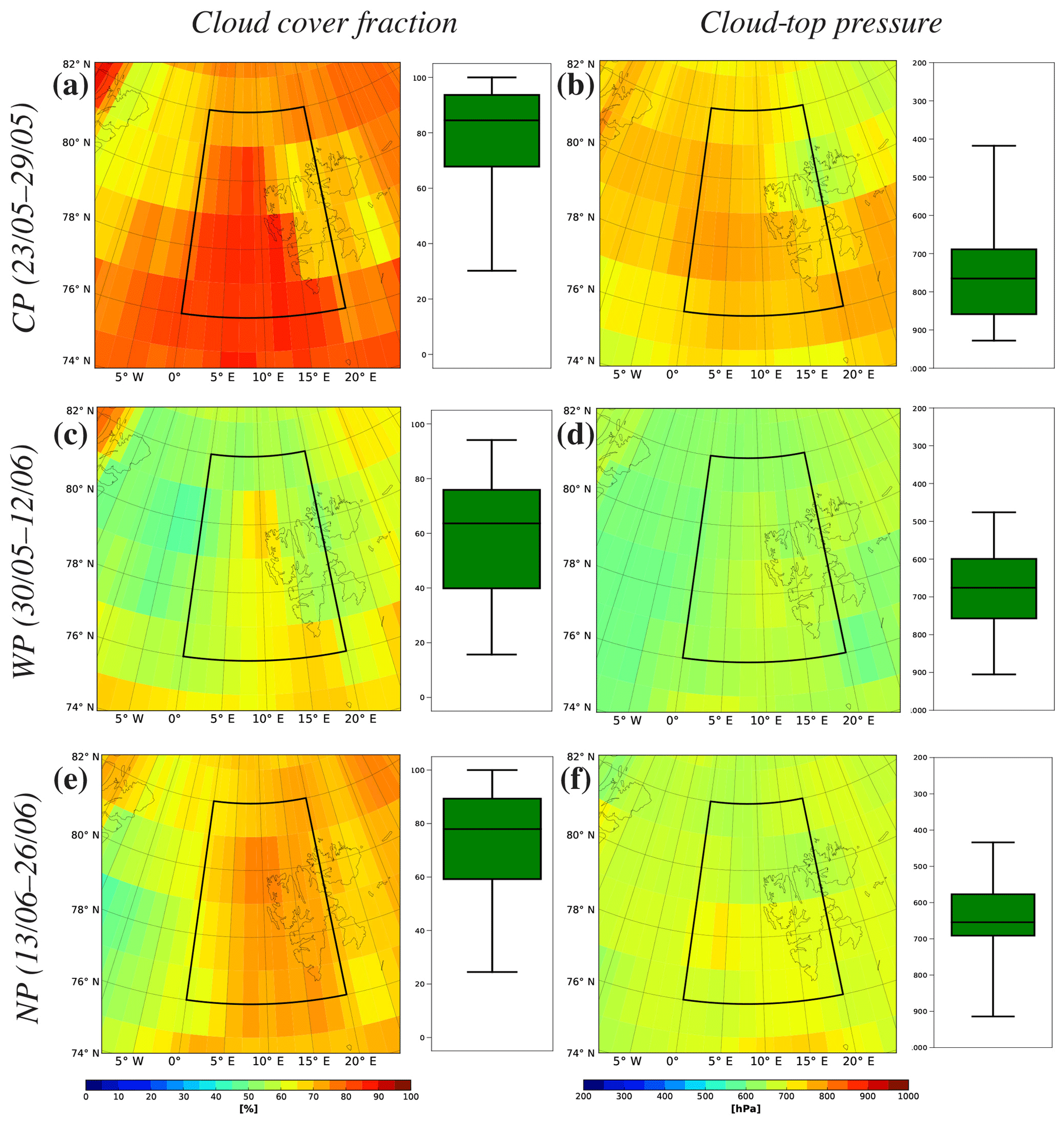
Figure 11Average (a, c, e) cloud cover fractions and (b, d, f) cloud-top pressures for each ACLOUD/PASCAL key period from IASI. Box plots represent averages over the central ACLOUD/PASCAL region (76–82∘ N, 0–20∘ E; black boxes in map panels), with ticks indicating the 5th and 95th percentiles. The key periods are defined as (a, b) the cold period (CP), (c, d) the warm period (WP), and (e, f) the normal period (NP).
Of the three key periods, the highest cloud cover fraction is observed during CP, with an average of about 85 % in the central ACLOUD/PASCAL region (Fig. 11a). In general, the highest cloud cover is observed over the open ocean (cf. Fig. 10a). This is in agreement with the results by Chan and Comiso (2013), who found a cloud cover fraction of about 88 % over open water across the whole Arctic and all seasons.
The high cloud cover during CP (Fig. 11a) was dominated by low-level clouds in the ACLOUD/PASCAL region with a median of the cloud-top pressure around 770 hPa (Fig. 11b). However, this median would have risen to 790 hPa (corresponding to an altitude of about 2 km) by the exclusion of the last CP day (29 May; not shown), typical for the MCAO discussed in Sect. 3.1–3.3. This cloud regime is also well in alignment with the reduced 700 hPa geopotential height and virtual potential temperature in Fig. 9a and b, indicating that the region was dominated by a northerly flow (cf. Fig. 7a). Subsequently, low-level clouds developed over the open ocean and the cloud-top longwave cooling led to a temperature inversion above the cloud (cf. Fig. 8a).
According to the time series of daily cloud cover fraction and top pressure (Fig. A3), the first 6 days of CP can clearly be classified as a stratus regime, which Eastman and Warren (2010) found to account for the majority of Arctic clouds in the May and June climatology. On the seventh and last day of CP (29 May), the change into another circulation regime is seen as the occurrence of high-level clouds (up to 350 hPa) increases in the central ACLOUD/PASCAL region due to their influence in its northern parts. Hence, no significant changes are observed near the surface (cf. Fig. 2b).
During WP, the lowest cloud cover fraction during ACLOUD/PASCAL was observed, with an average of about 65 % and a high spread between the 5th and 95th percentiles (Fig. 11c). Also, the individual days were characterized by a high spread in cloud cover fraction (Fig. A3a). While CP shows a meridional band with high values of cloud cover fraction associated with the location of open ocean, the spatial distribution changed strongly in WP, with the lowest cloud cover extending from the Fram Strait northward (Fig. 11c).
The lower cloud cover fraction during WP is associated with a change in cloud type, as cloud-top pressure values were more than 100 hPa lower than in CP (Fig. 11d compared to Fig. 11b), highlighting the highest clouds observed during ACLOUD/PASCAL. A value of 650 hPa is typical for mid-level clouds but can also result from a mixture of high- and low-level clouds. Average cloud-top pressure values were also more homogeneous over the Nordic Seas in WP compared to CP. Clouds were then likely associated with synoptic disturbances, which brought moister air masses from both westerly and easterly directions (cf. Fig. 7b).
The cloud cover fraction and cloud-top pressure in NP were in between those of CP and WP, with averages of about 80 % (Fig. 11e) and 700 hPa (Fig. 11f), respectively, but with larger spread in cloud-top pressure. The strong variability was also observed on a day-to-day basis (Fig. A3), which was caused by a mix of low-, mid-, and high-level clouds. During this period, the airflow was dominantly northwesterly, and the proportion of low-level clouds increased with respect to WP.
Overall, the observed cloud cover fraction between 70 % and 80 % during ACLOUD/PASCAL is in agreement with previous studies in the Arctic (Chan and Comiso, 2013; Eastman and Warren, 2010). Specifically for the Svalbard region, Mioche et al. (2015) found an average cloudiness of about 80 % for May and June using the most accurate vertical profiling satellite instruments. However, the analysis of the ACLOUD/PASCAL measurement period revealed that cloud characteristics show strong variability in space and time differing from the climatological distribution, with enhanced cloudiness over the open ocean southwest of Svalbard, while cloud cover fraction over ice-covered areas was found to be lower for most of the time. The highest contrast of cloudiness over these different surfaces is observed during CP, when the MCAO continuously triggered the formation of clouds over the warm open water. Mioche et al. (2015) identified these clouds predominantly as mixed-phase clouds (up to 60 % of all clouds). As passive satellite sensors have difficulties identifying cloud phase and multi-layer clouds, this will be investigated in more detail using other ACLOUD/PASCAL observations.
Similarly, a more complete picture of fog conditions will be made possible from the analysis of the wealth of ground and airborne remote sensing observations during ACLOUD/PASCAL. It is not possible to infer fog conditions from the satellite observations, as a high cloud-top pressure could either be related to low stratus or high fog conditions. Furthermore, due to the strong topographical influence on their location, observations from Ny-Ålesund are not representative of the ACLOUD/PASCAL region. The ice-attached Polarstern had a more representative location, from which visual observations are available. Here, fog was observed into the days of 6 and 8 June, as well as on 12 June. However, the visibility was mostly around 5 km and never fell below 500 m, indicating that low-hanging stratus clouds rather than fog were present most of the time.
In this section, we present the ACLOUD/PASCAL synoptic data in regional and climatological contexts in Sect. 5.1, 5.2, and 5.3. Additionally, the data are compared to other relevant Arctic field campaigns in Sect. 5.4.
5.1 Large-scale circulation indices
Two of the large-scale atmospheric indices, Arctic oscillation (Thompson and Wallace, 1998) and Arctic dipole (Wang et al., 2009; Wu et al., 2006), represent the first and second leading empirical orthogonal function (EOF) modes of the daily 1000 hPa geopotential height anomalies poleward of 20 and 70∘ N, respectively, normalized by the standard deviation of the monthly index. Another important circulation pattern in the Northern Hemisphere is the North Atlantic Oscillation (NAO), which is characterized by a pronounced north–south dipole in sea level pressure across the North Atlantic. The NAO is in this respect very similar to the AO but without the centers of action – the Aleutian Low and the Pacific High – over the Pacific Ocean. Accordingly, AO and NAO are closely related, with NAO actually being considered the regional occurrence of the hemisphere-wide pattern of AO (Thompson and Wallace, 1998). The analysis therefore focused on AO to provide broader information on the large-scale dynamics.
AO and AD are measures of the zonal and meridional wind patterns. AO describes the variability in the strength of the polar vortex. A positive AO index is associated with a lower-than-average pressure over the Arctic, a strong polar vortex, and a mainly zonal jet structure. A cold polar air mass is therefore more confined and located further poleward. In contrast, a negative AO index is linked to higher-than-average pressure over the Arctic, a weaker vortex, and a stronger meridional component of the jet stream. As a result, positive AO indices correlate with more numerous and deeper cyclones in the Arctic region, with storm tracks being shifted to the north (Simmonds et al., 2008). Conversely, negative indices are associated with more frequent blocking high events and persistent weather conditions, as well as with more likely MCAO events mainly in winter and spring (Overland et al., 2015). Toward summer, the AO pattern is displaced further northward and the meridional extent of its signal is considerably reduced (Ogi et al., 2004). A negative AO circulation in summer is nevertheless still supposed to cause substantial surface and tropospheric cooling and enhanced precipitation in midlatitudes (Hu and Feng, 2010; Wu et al., 2016).
A positive AD index is associated with a positive surface pressure anomaly over the Beaufort Sea, the Canadian Arctic archipelago, and Greenland, as well as a negative surface pressure anomaly over the Kara and Laptev seas. It is related to enhanced geostrophic wind flow from the Bering Strait toward the North Pole and across the Fram Strait, causing sea ice export out of the Arctic basin via the Fram Strait and the northern Barents Sea. A negative AD index is related to a lower-than-average surface pressure over the Beaufort Sea and Greenland, a higher-than-average surface pressure over northeast Eurasia, and enhanced poleward geostrophic wind flow (Wang et al., 2009). Since the 2000s, AO is less correlated with Arctic sea ice variability than AD. A positive AD is considered the main driver of Arctic sea ice export, regardless of the sign of AO (Overland et al., 2012; Smedsrud et al., 2017; Thompson and Wallace, 2001; Wang et al., 2009).
However, the connection between AD and Arctic sea ice drift is not always straightforward since the pressure pattern affecting AD may be orientated off the direction of the Transpolar Drift Stream, as pointed out by Overland and Wang (2010). Furthermore, the AD index is sensitive to the time period and geographical area considered in the calculation and is also dependent on the reanalysis data used. Meridional circulation indices based on the mean sea level pressure gradient across the Fram Strait or the Transpolar Drift Stream can provide a better quantitative relationship between the atmospheric forcing and sea ice drift speed throughout the year. Nevertheless, in summer, when the axis of the AD pattern is usually oriented along the Fram Strait, the AD index is found to correlate well with the sea ice evolution in the Fram Strait/Svalbard area (Vihma et al., 2012), which is the focus of the following qualitative analysis.
The analysis focuses on the variability of the AO and AD indices over the ACLOUD/PASCAL measurement and key periods, as well as corresponding periods over 1998–2016. This is shown in Fig. 12, which brings the ACLOUD/PASCAL measurements into a larger context. While the base period used in the analysis extends back to 1979, the AO and AD indices are presented for the last 20 years when the Arctic amplification became more prominent (Serreze and Barry, 2011). This allows a more relevant comparison to the 2017 ACLOUD/PASCAL campaign.
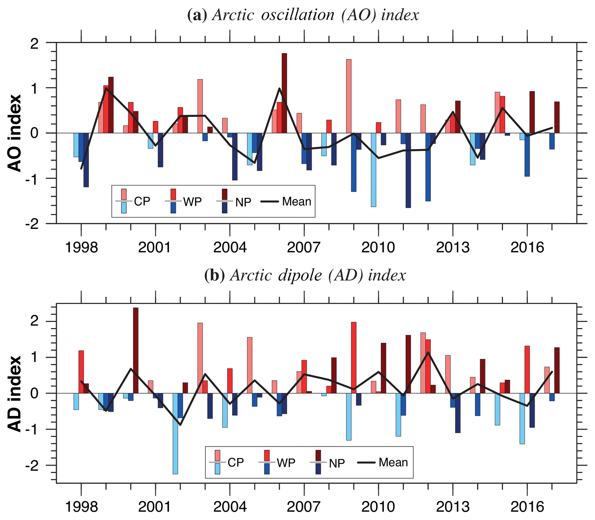
Figure 12Time series of (a) Arctic oscillation (AO) and (b) Arctic dipole (AD) indices for the Northern Hemisphere over the ACLOUD/PASCAL comparison period (1998–2017) based on ERA-I data. Lines and bars indicate campaign and key period averages, respectively. These are defined as 23 May–26 June (mean), 23–29 May (the cold period; CP), 30 May–12 June (the warm period; WP), and 13–26 June (the normal period; NP), respectively.
For the comparison period (1998–2017), the AO index varied between −1.8 and +1.9, with a relatively regular year-to-year alternation between positive and negative phases until 2006 (Fig. 12a). After 2006, the fraction of years with positive AO index for the periods 30 May–12 June (corresponding to WP) and 13–26 June (corresponding to NP) decreased from about a half to about a third (36 % and 27 %, respectively). The fraction of positive AO index values in the period 23–29 May, corresponding to CP, remained stable at about 55 %. Nevertheless, negative values of the AO index dominated from 2007, with minima down to −1.8 in the three consecutive years (2010 to 2012) and in 2016. This shift toward a more dominant negative phase of the AO pattern has been already reported in a range of recent studies and is supposed to result from the Arctic amplification (Overland et al., 2015). During ACLOUD/PASCAL in 2017, barely positive and moderate negative AO indices were found during CP and WP, respectively, which can be interpreted as an indication of enhanced meridional air mass transfer during the MCAO and WAA (cf. Sect. 3.3). A strongly positive value of +0.9 was observed for NP.
The AD index ranged between values of −2.2 and +2.3 in the analyzed period (1998–2017), with the largest positive values occurring in the corresponding NP of 2000 and negative values in the corresponding CP of 2002 (Fig. 12b). Since 2007, the AD index has mainly been positive, with strongly positive values between +1 and +2 dominating all corresponding key periods. The number of occurrence and magnitude of positive AD indices have increased in these years, especially in the corresponding WP by about 40 %. Positive AD index values occurred only in the years 2007, 2010, and 2012. This matches the observation that there has been an increase in sea ice export through the Fram Strait of approximately 6 % per decade since 1979, with the highest trend of 11 % in spring and summer (Smedsrud et al., 2017). All years with strongly positive AD indices in Fig. 12b were among the years with record low sea ice extent during the last decade. Nonetheless, the number of strongly negative AD index values (below −0.8) has increased by more than 30 % over the last 11 years. Since 2013, more negative AD indices have returned. These results indicate a general enhancement of poleward and equatorward airflow in early summer in recent years. During ACLOUD/PASCAL in 2017, the AD index was positive in CP and strongly positive in NP with a value of +1.3. A slightly negative index is found for WP. This evolution of the large-scale circulation in 2017 explains well the sea ice conditions in the Fram Strait observed during ACLOUD/PASCAL, as described in Sect. 4.3.
5.2 Seasonal characteristics
The onset of snowmelt is a key parameter for Arctic amplification, as it determines the seasonal change of the surface energy budget. Due to the melt of snow and later sea ice, radiative and sensible heat is efficiently stored in form of latent heat in the Arctic Ocean. The date of early snowmelt onset is retrieved from passive microwave satellite observations over sea ice (Markus et al., 2009). This date represents the first day under melting conditions and is plotted jointly for both the climatological period and the 2017 deviation from the climatological period in Fig. 13.
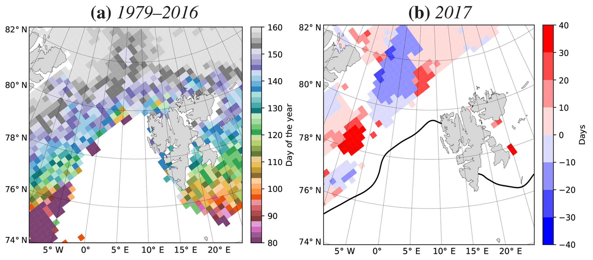
Figure 13(a) Climatology (1979–2016) and (b) anomaly relative to the climatology (2017 minus 1979–2016) of snowmelt onset date based on NASA GSFC data. In panel (b), white shading south of the 2017 sea ice edge (line) indicates open water.
Arctic-wide, the climatology for 1979–2016 shows a continuous increase in the date of melt onset with latitude from around day of the year 100 (10 April) in the outer regions to later than 160 (9 June) in the central Arctic Ocean (not shown). In the Fram Strait, the climatological transition zone from early to late onset of melt is much more spatially compressed, starting around day of the year 140 (20 May), with a narrower area of onset about 10 days later in the area of the West Spitsbergen Current west of the Yermak Plateau (around 82∘ N, 5∘ E; Aagaard et al., 1987; Fig. 13a).
In 2017, the snowmelt started 10–30 days earlier than normal in the eastern vicinity of the Northeast Water Polynya (see discussion in Sect. 4.3; Fig. 13b). This early onset is also found in other recent years (not shown). In contrast, the snow on sea ice both west and east of this area started melting 10–30 days later in 2017 relative to climatology.
5.3 Anomalous events
Building on Fig. 6 (see discussion in Sect. 3.3), Fig. 14 shows the occurrences, duration, and intensity of MCAOs and WAA over the ACLOUD/PASCAL comparison period (23 May–26 June 1998–2017). As for the AO and AD indices in Fig. 12, we present the most recent and relevant 20 years in Fig. 14, even though calculations were made over the climatological period (1979–2017).
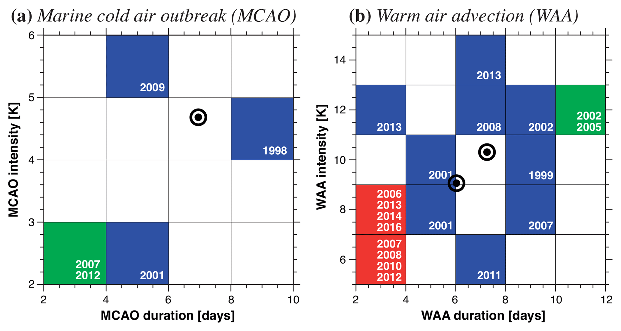
Figure 14(a) Marine cold air outbreak (MCAO) and (b) warm air advection (WAA) durations and intensities for the eastern Greenland Sea (75.00–80.25∘ N, 4.50–10.50∘ E) over the ACLOUD/PASCAL comparison period (23 May–26 June 1998–2017), based on ERA-I data. Colored boxes represent the number of MCAO and WAA events over 1998–2016, with specific years indicated in white. Black bullseye symbols represent 2017 events.
We identified six MCAO events within the 20-year ACLOUD/PASCAL comparison period (Fig. 14a). These lasted from 2 to 8 days and had intensities of 2.5–5.6 K. In 2017, one MCAO event was observed (cf. Fig. 6), which was in the upper part of the climatological range, lasting 7 days with an intensity of 4.7 K. This event was remarkable for this season, showing well-developed convective rolls and cloud streets in satellite images, but still was weak compared to cold season MCAOs, when indices reach more than 10 K (Chechin and Lüpkes, 2017; Fletcher et al., 2016).
Warm air advection is more common in early summer, with 21 events recognized over the ACLOUD/PASCAL comparison period (Fig. 14b). Duration and strengths of these reached up to 12 days and 14 K, respectively, although the majority lasted less than 8 days and were weaker than 9 K. In 2017, two moderate WAA events took place (cf. Fig. 6). These lasted 6 and 7 days and had intensities of 9.1 to 10.3 K, respectively.
5.4 Other campaigns
The few observations in the ACLOUD/PASCAL region partly explain the motivation for the field campaigns. Paradoxically, this also makes it hard to compare the data shown in this paper to other studies. Nevertheless, with differences in years, seasons, locations, and set-ups taken into account, such a comparison is still relevant for understanding the rapidly changing Arctic climate system. In this way, ACLOUD/PASCAL provides an important addition to earlier campaigns, as well as serving as a benchmark for upcoming Arctic field campaigns (e.g., the Multidisciplinary drifting Observatory for the Study of Arctic Climate; MOSAiC; IASC, 2016).
SHEBA (see Fig. 1a) was the first field campaign to include a full year of Arctic measurements (Uttal et al., 2002). Taking place from October 1997 to October 1998, its main objective was to advance the understanding of the coupled ocean–ice–atmosphere processes in models. While taking place in the ice pack of the Beaufort Sea on the opposing side of the Arctic Ocean, some comparisons to ACLOUD/PASCAL can still be made. During May and June 1998, temperature inversion heights of about 200–700 m and persistent cloudiness (80 %–100 %) characterized the SHEBA ice camp (Uttal et al., 2002). Over the same months in 2017, we observed inversion heights both shallower (about 100 m) and deeper (about 1400 m) north of Svalbard (Fig. 5a), along with cloudy conditions in the whole region (Fig. 11). While there are considerable regional differences between the Beaufort Sea and the Fram Strait, the snowmelt season began 29 May and ended during the first half of June both during SHEBA and ACLOUD/PASCAL (Fig. 2b).
The drifting ice station Tara was in the central Arctic Ocean during the International Polar Year from September 2006 to September 2007 (see Fig. 1a) and thus within the trend of rapidly rising Arctic temperatures (Vihma et al., 2008). Even so, the summer (as defined by snow/sea ice temperature) started later at Tara than at SHEBA 9 years earlier: on 9 June compared to 30 May. Similarly, the mean profiles from April to August were warmer and moister during SHEBA (Vihma et al., 2008). These warmer conditions might be a result of the more northerly location of Tara compared to SHEBA. While also taking place mostly north of SHEBA, mean profiles during ACLOUD/PASCAL were typically warmer and moister than during SHEBA (Fig. 8), plausibly due to the relatively warm West Spitsbergen Current (Aagaard et al., 1987) and/or the more synoptic active Arctic North Atlantic sector of ACLOUD/PASCAL (Serreze et al., 1997).
The Swedish icebreaker Oden has been regularly deployed in the Atlantic sector of the Arctic Ocean over the last decades. It was used for the two expeditions (AOE-96 in July–September 1996 and AOE-2001 in June–August 2001), as well as the more recent ASCOS expedition in August–September 2008 (Tjernström et al., 2012; see Fig. 1a). While their main focus was on the late summer season, comparisons to the more recent ACLOUD/PASCAL campaign are still relevant due to the more southerly location and stronger influence of the Arctic amplification of the latter.
ASCOS was dominated by anticyclonic atmospheric circulation, while cyclonic circulation prevailed during AOE-96 and AOE-2001 (Tjernström et al., 2012). During the ACLOUD/PASCAL measurement period, we found strong daily variability (Video S1), with cyclonic and anticyclonic circulation governing CP and WP, respectively (Fig. 9a and c). Nevertheless, similar to ACLOUD/PASCAL (Fig. 7), significant differences in airflow regimes were also observed during ASCOS (Fig. 9 in Tjernström et al., 2012).
Similar to the AOE-96, SHEBA, AOE-2001, and ASCOS campaigns (Tjernström et al., 2012), we observed inversions and these mostly in the lowest kilometer in almost all profiles when Polarstern was located in the sea-ice-covered area (Fig. 5). Of the three mean profiles in Fig. 8, NP (i.e., the last and most representative key period) corresponds best to the profiles from AOE-96, SHEBA, AOE-2001, and ASCOS (Fig. 15a and b in Tjernström et al., 2012).
Most comparable to ACLOUD/PASCAL is the N-ICE2015 expedition (see Fig. 1a). This took place in the sea ice north of Svalbard and included sea ice drift measurements in winter and spring 2015 (Granskog et al., 2016). May and June temperature values and variability were similar in 2015 (Fig. 3b in Cohen et al., 2017) and 2017 (Fig. 2b here), with mostly lifted temperature inversions and surface-based humidity inversions (Fig. 3 in Kayser et al., 2017 compared to Fig. 5 here). As observed during SHEBA, Tara, and N-ICE2015 (Cohen et al., 2017), the summer began around the first week of June during ACLOUD/PASCAL (Fig. 2b here).
In general, ACLOUD/PASCAL was to a low degree influenced by synoptic cyclones, as indicated by the few significant changes in the temperature and humidity time series (Fig. 2b and c) in association with the changes in the pressure time series (Fig. 2a). In this respect, the conditions during N-ICE2015 were different, when a persistent and anomalous low pressure centered over the Barents Sea dominated the corresponding season (Cohen et al., 2017). In 2015, this caused more abrupt shifts in cloud cover due to the associated cyclonic circulation (Cohen et al., 2017; Graham et al., 2017; Kayser et al., 2017); in 2017, we observed the cloudiest conditions in association with cyclonic circulation (Figs. 9a and 11a). We also found no significant precipitation events to follow from pressure drops (Fig. 2a and c here compared to Fig. 3a in Cohen et al., 2017).
This paper provides an overview of the synoptic development during the ACLOUD airborne and PASCAL ship-based field campaigns, which took place near Svalbard from 23 May to 26 June 2017. This development is characterized by near-surface and upper-air meteorological observations, satellite, and model data.
Time series of the data from Ny-Ålesund (at 79∘ N, 12∘ E) and Polarstern ocean-crossing (in the Nordic Seas north of the Arctic Circle) and ice-attached locations (at about 82∘ N, 10∘ E) during the 35-day measurement period are presented and compared to the long-term near-surface and radiosonde measurements conducted in Ny-Ålesund. Additionally, we computed the MCAO index and compared this to its climatology of the region.
Relative to the long-term averages, we identified three key periods representative of the distinct synoptic states during the ACLOUD/PASCAL measurement period: (1) a cold period (CP; 23–29 May; 7 days), (2) a warm period (WP; 30 May–12 June; 14 days), and (3) a normal period (NP; 13–26 June; 14 days). These were characterized by (1) cold and dry Arctic air advected from the north, (2) warm and moist maritime air transported from the south and east, and (3) close-to-average temperate and moist air from a mixture of regions (but dominated by adiabatically warmed air from the west). The sea ice drift during ACLOUD/PASCAL was strongly influenced by the large-scale atmospheric circulation and featured an anomalous southerly sea ice edge in the Fram Strait, packing of the ice edge, and opening of the Northeast Water Polynya in CP, WP, and NP, respectively. Associated with the cold and dry Arctic airflow, low-level stratus clouds prevailed over the open ocean in CP, while the warm air advection coincided with complex cloud systems having considerable vertical extent in WP. NP showed a mix of both conditions. Thus, relative to the long-term observations, we found short-term variability in atmospheric circulation to dominate the weather condition during ACLOUD/PASCAL.
The work presented in this paper shows that the synoptic variability in this region and time period is found to largely determine the surface meteorology, atmospheric profiles, and the cloud distribution. This synoptic variability is connected to the large-scale atmospheric variability, which itself was strongly linked to the sea ice distribution during the ACLOUD/PASCAL period. The analysis confirmed the conclusion by Kayser et al. (2017), who suggested that observations above Ny-Ålesund are fairly representative of the middle-to-upper troposphere in the ACLOUD/PASCAL region. However, for understanding surface observations, the knowledge of the boundary layer variability is key.
Our focus was limited to the North Atlantic sector of the Arctic. Hence, the results presented here do not necessarily translate to the entire Arctic climate system because the regional differences are too large (Cavalieri and Parkinson, 2012; Koyama et al., 2017; Serreze et al., 2011). For example, sea ice coverage in the region was anomalously high and reached far south as a result of the strong southward drift during CP and, albeit weaker, still southward drifts during WP and NP. Nevertheless, considering the sparsely observed Arctic region, the extensive ACLOUD/PASCAL campaign offers unique measurements covering the entire tropospheric column, with observations over the open ocean, sea ice, and snow. Most measurements performed during ACLOUD/PASCAL will be continued in the framework of MOSAiC, including a 1-year ice drift of Polarstern and numerous aircraft- and ground-based activities. Thus, while MOSAiC will strongly benefit from the results and experiences gained from ACLOUD/PASCAL, the continuity of observations in this Arctic region is anticipated to considerably improve the understanding of the cloud-related processes in the Arctic atmosphere, as well as the ocean–ice–atmosphere interaction from turbulent and radiative energy fluxes. Ultimately, this will strengthen synoptic forecasting in weather models, benefiting actors beyond the scientific community.
The surface-based measurement data used in this paper are available through the information system PANGAEA (Maturilli, 2017a, b; Schmithüsen, 2017, 2018), hosted by AWI, Helmholtz Center for Polar and Marine Research and the Center for Marine Environmental Sciences (MARUM), UB, and the MET Norway web portal eKlima (http://eklima.met.no/, last access: 13 December 2017). Satellite data are accessible through UB (Spreen et al., 2017), NSIDC (Fetterer et al., 2018), OSI SAF (Lavergne et al., 2010), and the European Organisation for the Exploitation of Meteorological Satellites (EUMETSAT, 2017). Finally, the reanalysis and analysis data used in this study can be obtained from ECMWF (Dee et al., 2011). The authors have made software code that was developed for analysis of these data available in the Supplement.
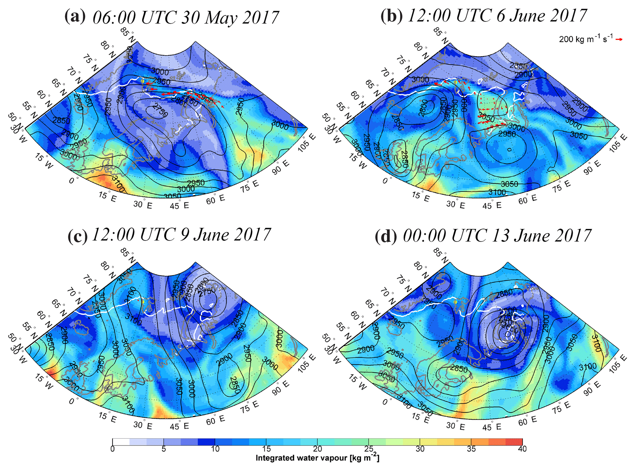
Figure A1Vertically integrated water vapor (IWV; in kg m−2; shading), 700 hPa geopotential height (in meters; black contours), and sea ice edge (defined by 15 % concentration; white line) for (a) 06:00 UTC on 30 May, (b) 12:00 UTC on 6 June, (c) 12:00 UTC on 9 June, and (d) 00:00 UTC on 13 June 2017, based on ERA-I data. In panels (a) and (b), red arrows indicate the IWV transport (IVT; in kg m−1 s−1) within the atmospheric rivers affecting Ny-Ålesund.
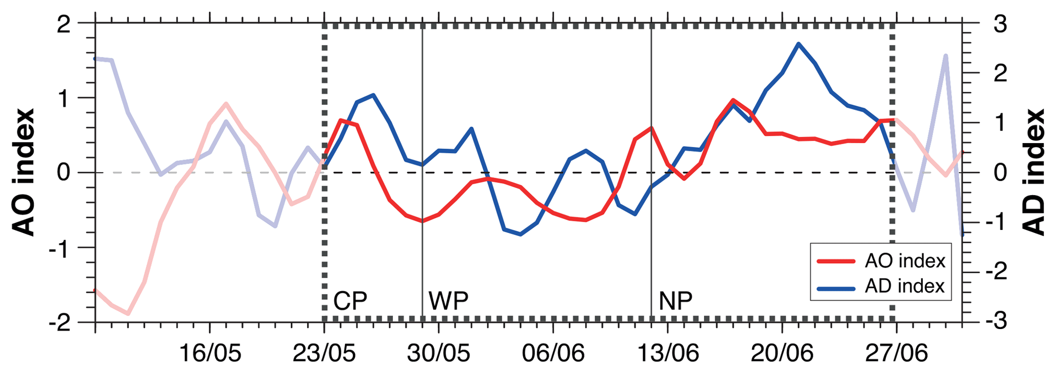
Figure A2Time series of daily Arctic oscillation (AO) and Arctic dipole (AD) indices over the ACLOUD/PASCAL extended period (9 May–1 July 2017), based on ERA-I data. Dotted boxes indicate the ACLOUD/PASCAL measurement period (23 May–26 June), while vertical lines separate the three key periods (CP, WP, and NP) defined in Sect. 4.
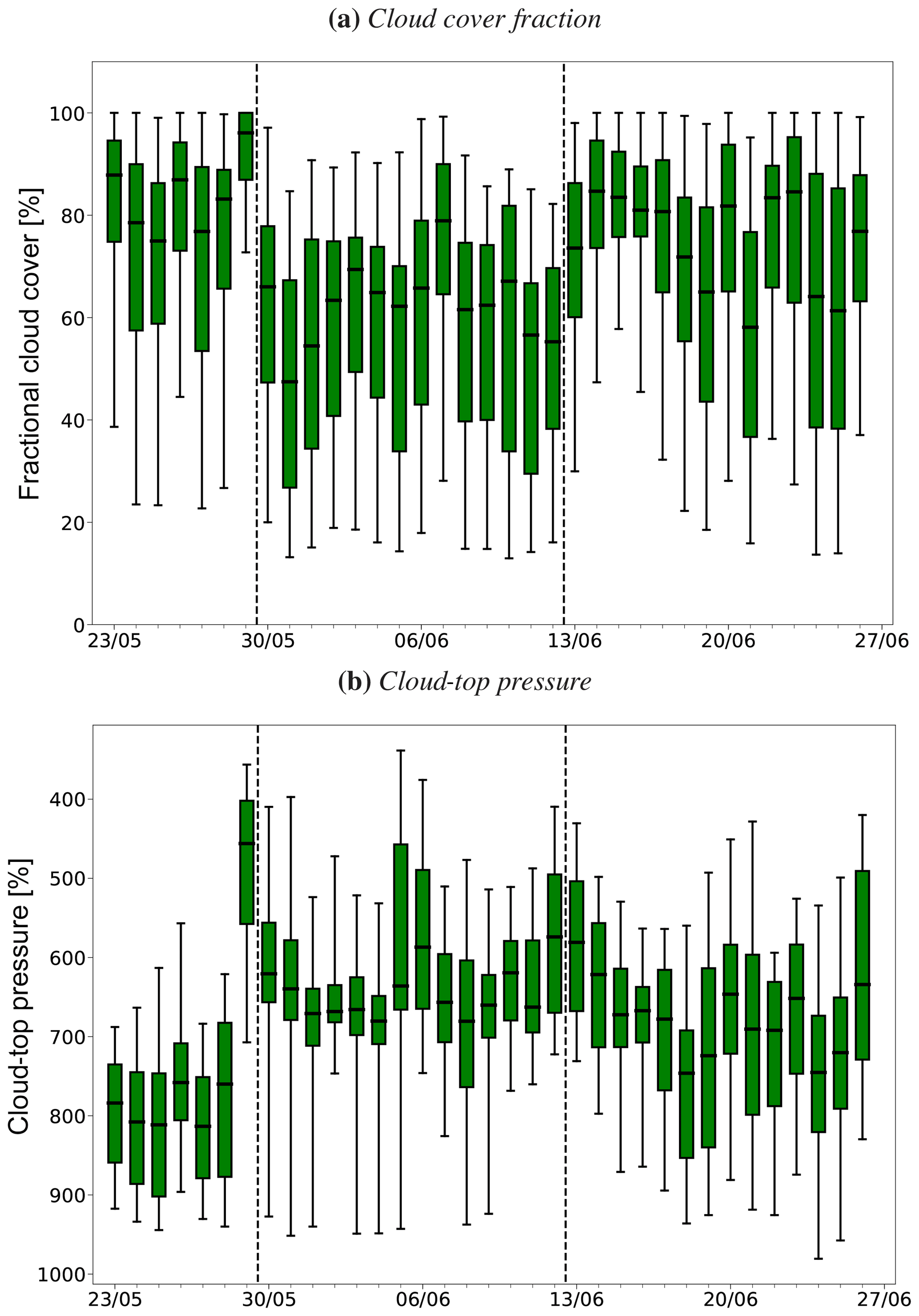
The supplement related to this article is available online at: https://doi.org/10.5194/acp-18-17995-2018-supplement.
EMK led the coordination and design of the study, analyzed data for and plotted Figs. 2 and 9 and Videos S1 and S2, and wrote all sections except for Sect. 1 based on the input from the co-authors. BH helped in the coordination and the design of the study, and also analyzed data, plotted, and provided descriptive text for Figs. 1, 6, 12, 14, and A2. SD helped in the design of the study, and also analyzed data, plotted, and provided descriptive text for Figs. 4, 5, and 8. HB and DK analyzed data, plotted, and provided descriptive text for Fig. 7. They also analyzed data and plotted Fig. 3, which CL provided descriptive text for. SC and MMe analyzed data, plotted, and provided descriptive text for Figs. 11 and A3. IVG and CV analyzed data, plotted, and provided descriptive text for Fig. A1. GH analyzed data, plotted, and provided descriptive text for Figs. 10 and 13. MMa and HS provided data from Ny-Ålesund and Polarstern, respectively. AR wrote Sect. 1. In addition to the other authors, AE, AM, and MW evaluated the study and paper.
The authors declare that they have no conflict of interest.
This article is part of the special issue “Arctic mixed-phase clouds as studied during the ACLOUD/PASCAL campaigns in the framework of (AC)3 (ACP/AMT inter-journal SI)”. It is not associated with a conference.
We gratefully acknowledge the funding by the German Research Foundation
(Deutsche Forschungsgemeinschaft; DFG) for the Transregional Collaborative
Research Center “ArctiC Amplification: Climate Relevant Atmospheric and
SurfaCe Processes, and Feedback Mechanisms (AC)3” (TRR 172, project no.
268020496). We thank David C. Strack for providing data used in Fig. 11,
as well as Malte Gerken and Catalin Patiliea for preparing plots used in
Figs. 10 and 13,
respectively. Christian Melsheimer provided the algorithm used in Videos S1 and S2.
Markus Kayser should also be mentioned for valuable comments on an earlier
version of this paper. Marc Rautenhaus is acknowledged for providing the
Mission Support System (Rautenhaus et al., 2012) for flight planning
during ACLOUD, as well as Jörn Ungermann and Reimar Bauer for technical
support. We wish to thank the reviewers for constructive suggestions that
improved the manuscript.
Edited by: Amy Solomon
Reviewed by: Timo Vihma and Lana Cohen
Aagaard, K., Foldvik, A., and Hillman, S.: The West Spitsbergen Current: Disposition and water mass transformation, J. Geophys. Res.-Oceans, 92, 3778–3784, https://doi.org/10.1029/JC092iC04p03778, 1987. a, b
Akperov, M., Rinke, A., Mokhov, I., Matthes, H., Semenov, V., Adakudlu, M., Cassano, J., Christensen, J., Dembitskaya, M., Dethloff, K., Fettweis, X., Glisan, J., Gutjahr, O., Heinemann, G., Koenig, T., Koldunov, N., Laprise, R., Mottram, R., Nikiéma, O., Scinocca, J., Sein, D., Sobolowski, S., Winger, K., and Zhang, W.: Cyclone activity in the Arctic from an ensemble of regional climate models (Arctic CORDEX), J. Geophys. Res.-Atmos., 123, 2537–2554, https://doi.org/10.1002/2017JD027703, 2018. a
Andreas, E., Claffy, K., and Makshtas, A.: Low-level atmospheric jets and inversions over the western Weddell Sea, Bound-Lay. Meteorol., 97, 459–486, https://doi.org/10.1023/A:1002793831076, 2000. a
Barton, N., Klein, S., and Boyle, J.: On the contribution of longwave radiation to global climate model biases in Arctic lower tropospheric stability, J. Climate, 27, 7250–7269, https://doi.org/10.1175/JCLI-D-14-00126.1, 2014. a
Bintanja, R., Graversen, R., and Hazeleger, W.: Arctic winter warming amplified by the thermal inversion and consequent low infrared cooling to space, Nat. Geosci., 4, 758, https://doi.org/10.1038/ngeo1285, 2011. a
Catto, J., Shaffrey, L., and Hodges, K.: Can climate models capture the structure of extratropical cyclones?, J. Climate, 23, 1621–1635, https://doi.org/10.1175/2009JCLI3318.1, 2010. a
Cavalieri, D. J. and Parkinson, C. L.: Arctic sea ice variability and trends, 1979–2010, The Cryosphere, 6, 881–889, https://doi.org/10.5194/tc-6-881-2012, 2012. a
Chan, M. and Comiso, J.: Arctic cloud characteristics as derived from MODIS, CALIPSO, and CloudSat, J. Climate, 26, 3285–3306, https://doi.org/10.1175/JCLI-D-12-00204.1, 2013. a, b
Chechin, D. and Lüpkes, C.: Boundary-layer development and low-level baroclinicity during high-latitude cold-air outbreaks: A simple model, Bound-Lay. Meteorol., 162, 91–116, https://doi.org/10.1007/s10546-016-0193-2, 2017. a
Chung, C. E., Cha, H., Vihma, T., Räisänen, P., and Decremer, D.: On the possibilities to use atmospheric reanalyses to evaluate the warming structure in the Arctic, Atmos. Chem. Phys., 13, 11209–11219, https://doi.org/10.5194/acp-13-11209-2013, 2013. a
CloudSat DPC: CloudSat News, available at: http://www.cloudsat.cira.colostate.edu/news (last access: 16 February 2018), 2017. a
Cohen, L., Hudson, S., Walden, V., Graham, R., and Granskog, M.: Meteorological conditions in a thinner Arctic sea ice regime from winter through summer during the Norwegian Young Sea Ice expedition (N-ICE2015), J. Geophys. Res.-Atmos., 122, 7235–7259, https://doi.org/10.1002/2016JD026034, 2017. a, b, c, d, e, f
Dahlke, S. and Maturilli, M.: Contribution of Atmospheric Advection to the Amplified Winter Warming in the Arctic North Atlantic Region, Adv. Meteorol.,8, 4928620, https://doi.org/10.1155/2017/4928620, 2017. a
de Boer, G., Shupe, M. D., Caldwell, P. M., Bauer, S. E., Persson, O., Boyle, J. S., Kelley, M., Klein, S. A., and Tjernström, M.: Near-surface meteorology during the Arctic Summer Cloud Ocean Study (ASCOS): evaluation of reanalyses and global climate models, Atmos. Chem. Phys., 14, 427–445, https://doi.org/10.5194/acp-14-427-2014, 2014. a
Dee, D., Uppala, S., Simmons, A., Berrisford, P., Poli, P., Kobayashi, S., Andrae, U., Balmaseda, M., Balsamo, G., Bauer, P., Bechtold, P., Beljaars, A., van de Berg, L., Bidlot, J., Bormann, N., Delsol, C., Dragani, R., Fuentes, M., Geer, A., Haimberger, L., Healy, S., Hersbach, H., Hólm, E., Isaksen, L., Kållberg, P., Köhler, M., Matricardi, M., McNally, A., Monge-Sanz, B., Morcrette, J.-J., Park, B.-K., Peubey, C., de Rosnay, P., Tavolato, C., Thépaut, J.-N., and Vitart, F.: The ERA-Interim reanalysis: Configuration and performance of the data assimilation system, Q. J. Roy. Meteor. Soc., 137, 553–597, https://doi.org/10.1002/qj.828, 2011. a, b
Devasthale, A., Sedlar, J., and Tjernström, M.: Characteristics of water-vapour inversions observed over the Arctic by Atmospheric Infrared Sounder (AIRS) and radiosondes, Atmos. Chem. Phys., 11, 9813–9823, https://doi.org/10.5194/acp-11-9813-2011, 2011. a
Eastman, R. and Warren, S.: Interannual variations of Arctic cloud types in relation to sea ice, J. Climate, 23, 4216–4232, https://doi.org/10.1175/2010JCLI3492.1, 2010. a, b
English, J., Gettelman, A., and Henderson, G.: Arctic radiative fluxes: Present-day biases and future projections in CMIP5 models, J. Climate, 28, 6019–6038, https://doi.org/10.1175/JCLI-D-14-00801.1, 2015. a
Etling, D.: Theoretische Meteorologie: Eine Einführung, Springer-Verlag, Berlin, Heidelberg, 3 edn., 2008. a
EUMETSAT: IASI Level 2: Product Guide, Tech. rep., EUMETSAT, Darmstadt, Germany, 2017. a, b, c
Fetterer, F., Knowles, K., Meier, W., Savoie, M., and Windnagel, A. K.: Sea ice index, version 3, Sea ice concentration and anomalies, available at: https://doi.org/10.7265/N5K072F8, 2018. a, b, c, d
Fletcher, J., Mason, S., and Jakob, C.: The climatology, meteorology, and boundary layer structure of marine cold air outbreaks in both hemispheres, J. Climate, 29, 1999–2014, https://doi.org/10.1175/JCLI-D-15-0268.1, 2016. a, b
Gorodetskaya, I., Tsukernik, M., Claes, K., Ralph, M., Neff, W., and Van Lipzig, N.: The role of atmospheric rivers in anomalous snow accumulation in East Antarctica, Geophys. Res. Lett., 41, 6199–6206, https://doi.org/10.1002/2014GL060881, 2014. a
Graham, R., Rinke, A., Cohen, L., Hudson, S., Walden, V., Granskog, M., Dorn, W., Kayser, M., and Maturilli, M.: A comparison of the two Arctic atmospheric winter states observed during N-ICE2015 and SHEBA, J. Geophys. Res.-Atmos., 122, 5716–5737, https://doi.org/10.1002/2016JD025475, 2017. a, b
Granskog, M., Assmy, P., Gerland, S., Spreen, G., Steen, H., and Smedsrud, L.: Arctic research on thin ice: Consequences of Arctic sea ice loss, Eos, 97, https://doi.org/10.1029/2016EO044097, 2016. a
Hanna, S.: The thickness of the planetary boundary layer, Atmos. Environ., 3, 519–536, https://doi.org/10.1016/0004-6981(69)90042-0, 1969. a
Hirdman, D., Sodemann, H., Eckhardt, S., Burkhart, J. F., Jefferson, A., Mefford, T., Quinn, P. K., Sharma, S., Ström, J., and Stohl, A.: Source identification of short-lived air pollutants in the Arctic using statistical analysis of measurement data and particle dispersion model output, Atmos. Chem. Phys., 10, 669–693, https://doi.org/10.5194/acp-10-669-2010, 2010. a
Hu, Q. and Feng, S.: Influence of the Arctic oscillation on central United States summer rainfall, J. Geophys. Res.-Atmos., 115, D01102, https://doi.org/10.1029/2009JD011805, 2010. a
Hyland, R. and Wexler, A.: Formulations for the thermodynamic properties of the saturated phases of H2O from 173.15 K to 473.15 K, ASHRAE Tran., 89, 500–519, 1983. a
IASC: MOSAiC: Multidisciplinary drifting Observatory for the Study of Arctic Climate – Science Plan, Tech. rep., International Arctic Science Committee, Akureyri, Iceland, 2016. a
Jakobson, E., Vihma, T., Palo, T., Jakobson, L., Keernik, H., and Jaagus, J.: Validation of atmospheric reanalyses over the central Arctic Ocean, Geophys. Res. Lett., 39, L10802, https://doi.org/10.1029/2012GL051591, 2012. a
Jeffries, M., Overland, J., and Perovich, D.: The Arctic shifts to a new normal, Phys. Today, 66, 35–40, https://doi.org/10.1063/PT.3.2147, 2013. a
Johansson, E., Devasthale, A., Tjernström, M., Ekman, A., and L'Ecuyer, T.: Response of the lower troposphere to moisture intrusions into the Arctic, Geophys. Res. Lett., 44, 2527–2536, https://doi.org/10.1002/2017GL072687, 2017. a
Kahl, J.: Characteristics of the low-level temperature inversion along the Alaskan Arctic coast, Int. J. Climatol., 10, 537–548, https://doi.org/10.1002/joc.3370100509, 1990. a
Karlsson, J. and Svensson, G.: Consequences of poor representation of Arctic sea-ice albedo and cloud-radiation interactions in the CMIP5 model ensemble, Geophys. Res. Lett., 40, 4374–4379, https://doi.org/10.1002/grl.50768, 2013. a
Kayser, M., Maturilli, M., Graham, R., Hudson, S., Rinke, A., Cohen, L., Kim, J.-H., Park, S.-J., Moon, W., and Granskog, M.: Vertical thermodynamic structure of the troposphere during the Norwegian young sea ICE expedition (N-ICE2015), J. Geophys. Res.-Atmos., 122, 10855–10872, https://doi.org/10.1002/2016JD026089, 2017. a, b, c, d, e, f
Kim, Y., Choi, Y.-S., Kim, B.-M., and Kim, H.: Influence of altered low cloud parameterizations for seasonal variation of Arctic cloud amount on climate feedbacks, Clim. Dynam., 47, 1661–1672, https://doi.org/10.1007/s00382-015-2926-1, 2016. a
Knudsen, E. M. and Walsh, J. E.: Northern Hemisphere storminess in the Norwegian Earth System Model (NorESM1-M), Geosci. Model Dev., 9, 2335–2355, https://doi.org/10.5194/gmd-9-2335-2016, 2016. a
Knudsen, E., Orsolini, Y., Furevik, T., and Hodges, K.: Observed anomalous atmospheric patterns in summers of unusual Arctic sea ice melt, J. Geophys. Res.-Atmos., 120, 2595–2611, https://doi.org/10.1002/2014JD022608, 2015. a
Kolstad, E.: Higher ocean wind speeds during marine cold air outbreaks, Q. J. Roy. Meteor. Soc., 143, 2084–2092, https://doi.org/10.1002/qj.3068, 2017. a, b, c
Koyama, T., Stroeve, J., Cassano, J., and Crawford, A.: Sea ice loss and Arctic cyclone activity from 1979 to 2014, J. Climate, 30, 4735–4754, https://doi.org/10.1175/JCLI-D-16-0542.1, 2017. a
Lavanant, L., Fourrié, N., Gambacorta, A., Grieco, G., Heilliette, S., Hilton, F., Kim, M.-J., McNally, A., Nishihata, H., Pavelin, E., and Rabier, F.: Comparison of cloud products within IASI footprints for the assimilation of cloudy radiances, Q. J. Roy. Meteor. Soc., 137, 1988–2003, https://doi.org/10.1002/qj.917, 2011. a, b
Lavergne, T., Eastwood, S., Teffah, Z., Schyberg, H., and Breivik, L.-A.: Sea ice motion from low-resolution satellite sensors: An alternative method and its validation in the Arctic, J. Geophys. Res.-Oceans, 115, C10032, https://doi.org/10.1029/2009JC005958, 2010. a, b
Lesins, G., Duck, T., and Drummond, J.: Climate trends at Eureka in the Canadian high Arctic, Atmos. Ocean, 48, 59–80, https://doi.org/10.3137/AO1103.2010, 2010. a
Lindsay, R., Wensnahan, M., Schweiger, A., and Zhang, J.: Evaluation of seven different atmospheric reanalysis products in the Arctic, J. Climate, 27, 2588–2606, 2014. a
Lüpkes, C., Vihma, T., Jakobson, E., and König-Langlo, G.and Tetzlaff, A.: Meteorological observations from ship cruises during summer to the central Arctic: A comparison with reanalysis data, Geophys. Res. Lett., 37, L09810, https://doi.org/10.1029/2010GL042724, 2010. a
Macke, A. and Flores, H.: The Expeditions PS106/1 and 2 of the Research Vessel POLARSTERN to the Arctic Ocean in 2017, Berichte zur Polar- und Meeresforschung = Reports on polar and marine research, Tech. rep., Alfred Wegener Institute for Polar and Marine Research, Bremerhaven, Germany, https://doi.org/10.2312/BzPM_0719_2018, 2018. a, b, c
Markus, T., Stroeve, J., and Miller, J.: Recent changes in Arctic sea ice melt onset, freezeup, and melt season length, J. Geophys. Res.-Oceans, 114, C12024, https://doi.org/10.1029/2009JC005436, 2009. a, b
Maturilli, M.: High resolution radiosonde measurements from station Ny-Ålesund (2017-06), https://doi.org/10.1594/PANGAEA.879822, 2017a. a, b
Maturilli, M.: High resolution radiosonde measurements from station Ny-Ålesund (2017-05), https://doi.org/10.1594/PANGAEA.879820, 2017b. a, b
Maturilli, M. and Kayser, M.: Arctic warming, moisture increase and circulation changes observed in the Ny-Ålesund homogenized radiosonde record, Theor. Appl. Climatol., 130, 1–17, https://doi.org/10.1007/s00704-016-1864-0, 2017. a, b
Maturilli, M., Herber, A., and König-Langlo, G.: Climatology and time series of surface meteorology in Ny-Ålesund, Svalbard, Earth Syst. Sci. Data, 5, 155–163, https://doi.org/10.5194/essd-5-155-2013, 2013. a
Maturilli, M., Herber, A., and König-Langlo, G.: Surface radiation climatology for Ny-Ålesund, Svalbard (78.9∘ N), basic observations for trend detection, Theor. Appl. Climatol., 120, 331–339, https://doi.org/10.1007/s00704-014-1173-4, 2015. a
McIlhattan, E., L'Ecuyer, T., and Miller, N.: Observational evidence linking arctic supercooled liquid cloud biases in CESM to snowfall processes, J. Climate, 30, 4477–4495, https://doi.org/10.1175/JCLI-D-16-0666.1, 2017. a
Mioche, G., Jourdan, O., Ceccaldi, M., and Delanoë, J.: Variability of mixed-phase clouds in the Arctic with a focus on the Svalbard region: a study based on spaceborne active remote sensing, Atmos. Chem. Phys., 15, 2445–2461, https://doi.org/10.5194/acp-15-2445-2015, 2015. a, b
Morrison, H., Zuidema, P., Ackerman, A., Avramov, A., De Boer, G., Fan, J., Fridlind, A., Hashino, T., Harrington, J., Luo, Y., Ovchinnikov, M., and Shipway, B.: Intercomparison of cloud model simulations of Arctic mixed-phase boundary layer clouds observed during SHEBA/FIRE-ACE, J. Adv. Model. Earth Sy., 3, M06003, https://doi.org/10.1029/2011MS000066, 2011. a
Nash, D., Waliser, D., Guan, B., Ye, H., and Ralph, F.: The role of atmospheric rivers in extratropical and polar hydroclimate, J. Geophys. Res.-Atmos., 123, 6804–6821, https://doi.org/10.1029/2017JD028130, 2018. a
Ogi, M., Yamazaki, K., and Tachibana, Y.: The summertime annular mode in the Northern Hemisphere and its linkage to the winter mode, J. Geophys. Res.-Atmos., 109, D20114, https://doi.org/10.1029/2004JD004514, 2004. a
Overland, J. and Wang, M.: Large-scale atmospheric circulation changes are associated with the recent loss of Arctic sea ice, Tellus A, 62, 1–9, https://doi.org/10.1111/j.1600-0870.2009.00421.x, 2010. a
Overland, J., Francis, J., Hanna, E., and Wang, M.: The recent shift in early summer Arctic atmospheric circulation, Geophys. Res. Lett., 39, L19804, https://doi.org/10.1029/2012GL053268, 2012. a
Overland, J., Francis, J., Hall, R., Hanna, E., Kim, S.-J., and Vihma, T.: The melting Arctic and midlatitude weather patterns: Are they connected?, J. Climate, 28, 7917–7932, https://doi.org/10.1175/JCLI-D-14-00822.1, 2015. a, b
Papritz, L., Pfahl, S., Sodemann, H., and Wernli, H.: A climatology of cold air outbreaks and their impact on air–sea heat fluxes in the high-latitude South Pacific, J. Climate, 28, 342–364, https://doi.org/10.1175/JCLI-D-14-00482.1, 2015. a
Pithan, F. and Mauritsen, T.: Arctic amplification dominated by temperature feedbacks in contemporary climate models, Nat. Geosci., 7, 181, https://doi.org/10.1038/ngeo2071, 2014. a
Pithan, F., Medeiros, B., and Mauritsen, T.: Mixed-phase clouds cause climate model biases in Arctic wintertime temperature inversions, Clim. Dynam., 43, 289–303, https://doi.org/10.1007/s00382-013-1964-9, 2014. a, b
Rautenhaus, M., Bauer, G., and Dörnbrack, A.: A web service based tool to plan atmospheric research flights, Geosci. Model Dev., 5, 55–71, https://doi.org/10.5194/gmd-5-55-2012, 2012. a
Schmithüsen, H.: Upper air soundings during POLARSTERN cruise PS106.1 (ARK-XXXI/1.1), https://doi.org/10.1594/PANGAEA.882736, 2017. a, b
Schmithüsen, H.: Continuous meteorological surface measurement during POLARSTERN cruise PS106.1 (ARK-XXXI/1.1), https://doi.org/10.1594/PANGAEA.882616, 2018. a, b
Schneider, W. and Budéus, G.: Summary of the Northeast Water polynya formation and development (Greenland Sea), J. Marine Syst., 10, 107–122, https://doi.org/10.1016/S0924-7963(96)00075-9, 1997. a
Sedlar, J., Shupe, M. D., and Tjernström, M.: On the relationship between thermodynamic structure and cloud top, and its climate significance in the Arctic, J. Climate, 25, 2374–2393, https://doi.org/10.1175/JCLI-D-11-00186.1, 2012. a
Seibert, P. and Frank, A.: Source-receptor matrix calculation with a Lagrangian particle dispersion model in backward mode, Atmos. Chem. Phys., 4, 51–63, https://doi.org/10.5194/acp-4-51-2004, 2004. a
Serreze, M. and Barry, R.: Processes and impacts of Arctic amplification: A research synthesis, Global Planet. Change, 77, 85–96, https://doi.org/10.1016/j.gloplacha.2011.03.004, 2011. a, b
Serreze, M., Carse, F., Barry, R., and Rogers, J.: Icelandic low cyclone activity: Climatological features, linkages with the NAO, and relationships with recent changes in the Northern Hemisphere circulation, J. Climate, 10, 453–464, https://doi.org/10.1175/1520-0442(1997)010<0453:ILCACF>2.0.CO;2, 1997. a, b
Serreze, M., Barrett, A., and Cassano, J.: Circulation and surface controls on the lower tropospheric air temperature field of the Arctic, J. Geophys. Res.-Atmos., 116, D07104, https://doi.org/10.1029/2010JD015127, 2011. a
Simmonds, I., Burke, C., and Keay, K.: Arctic climate change as manifest in cyclone behavior, J. Climate, 21, 5777–5796, https://doi.org/10.1175/2008JCLI2366.1, 2008. a
Smedsrud, L. H., Halvorsen, M. H., Stroeve, J. C., Zhang, R., and Kloster, K.: Fram Strait sea ice export variability and September Arctic sea ice extent over the last 80 years, The Cryosphere, 11, 65–79, https://doi.org/10.5194/tc-11-65-2017, 2017. a, b
Solomon, A., Shupe, M. D., Persson, P. O. G., and Morrison, H.: Moisture and dynamical interactions maintaining decoupled Arctic mixed-phase stratocumulus in the presence of a humidity inversion, Atmos. Chem. Phys., 11, 10127–10148, https://doi.org/10.5194/acp-11-10127-2011, 2011. a
Sorteberg, A. and Walsh, J.: Seasonal cyclone variability at 70∘ N and its impact on moisture transport into the Arctic, Tellus A, 60, 570–586, https://doi.org/10.1111/j.1600-0870.2008.00314.x, 2008. a
Spreen, G., Kaleschke, L., and Heygster, G.: Sea ice remote sensing using AMSR-E 89-GHz channels, J. Geophys. Res.-Oceans, 113, C02S03, https://doi.org/10.1029/2005JC003384, 2008. a
Spreen, G., Melsheimer, C., and Heygster, G.: Sea ice concentration, available at: https://seaice.uni-bremen.de/sea-ice-concentration/ (last access: 23 February 2018), 2017. a, b, c
Stephens, G., Vane, D., Boain, R., Mace, G., Sassen, K., Wang, Z., Illingworth, A., O'Connor, E., Rossow, W., Durden, S., Miller, S., Austin, R., Benedetti, A., Mitrescu, C., and the CloudSat Science Team: The CloudSat mission and the A-Train: A new dimension of space-based observations of clouds and precipitation, B. Am. Meteorol. Soc., 83, 1771–1790, https://doi.org/10.1175/BAMS-83-12-1771, 2002. a
Stocker, T., Qin, D., Plattner, G.-K., Tignor, M., Allen, S., Boschung, J., Nauels, A., Xia, Y., V., B., and Midgley, P. (eds.): Climate change 2013: The physical science basis. Contribution of Working Group I to the Fifth Assessment Report of the Intergovernmental Panel on Climate Change, Tech. rep., Intergovernmental Panel on Climate Change (IPCC), Cambridge, United Kingdom and New York, USA, 2013. a
Stohl, A., Forster, C., Frank, A., Seibert, P., and Wotawa, G.: Technical note: The Lagrangian particle dispersion model FLEXPART version 6.2, Atmos. Chem. Phys., 5, 2461–2474, https://doi.org/10.5194/acp-5-2461-2005, 2005. a, b, c
Stramler, K., Del Genio, A., and Rossow, W.: Synoptically driven Arctic winter states, J. Climate, 24, 1747–1762, https://doi.org/10.1175/2010JCLI3817.1, 2011. a
Stubenrauch, C. J., Feofilov, A. G., Protopapadaki, S. E., and Armante, R.: Cloud climatologies from the infrared sounders AIRS and IASI: strengths and applications, Atmos. Chem. Phys., 17, 13625–13644, https://doi.org/10.5194/acp-17-13625-2017, 2017. a
Svensson, G. and Lindvall, J.: Evaluation of near-surface variables and the vertical structure of the boundary layer in CMIP5 models, J. Climate, 28, 5233–5253, https://doi.org/10.1175/JCLI-D-14-00596.1, 2015. a
Tetzlaff, A., Lüpkes, C., Birnbaum, G., Hartmann, J., Nygård, T., and Vihma, T.: Brief Communication: Trends in sea ice extent north of Svalbard and its impact on cold air outbreaks as observed in spring 2013, The Cryosphere, 8, 1757–1762, https://doi.org/10.5194/tc-8-1757-2014, 2014. a
Thompson, D. and Wallace, J.: The Arctic oscillation signature in the wintertime geopotential height and temperature fields, Geophys. Res. Lett., 25, 1297–1300, https://doi.org/10.1029/98GL00950, 1998. a, b
Thompson, D. and Wallace, J.: Regional climate impacts of the Northern Hemisphere annular mode, Science, 293, 85–89, https://doi.org/10.1126/science.1058958, 2001. a
Tjernström, M., Sedlar, J., and Shupe, M.: How well do regional climate models reproduce radiation and clouds in the Arctic? An evaluation of ARCMIP simulations, J. Appl. Meteorol. Clim., 47, 2405–2422, https://doi.org/10.1175/2008JAMC1845.1, 2008. a
Tjernström, M., Birch, C. E., Brooks, I. M., Shupe, M. D., Persson, P. O. G., Sedlar, J., Mauritsen, T., Leck, C., Paatero, J., Szczodrak, M., and Wheeler, C. R.: Meteorological conditions in the central Arctic summer during the Arctic Summer Cloud Ocean Study (ASCOS), Atmos. Chem. Phys., 12, 6863–6889, https://doi.org/10.5194/acp-12-6863-2012, 2012. a, b, c, d, e
Tjernström, M., Shupe, M., Brooks, I., Persson, P., Prytherch, J., Salisbury, D., Sedlar, J., Achtert, P., Brooks, B., Johnston, P., Sotiropoulou, G., and Wolfe, D.: Warm-air advection, air mass transformation and fog causes rapid ice melt, Geophys. Res. Lett., 42, 5594–5602, https://doi.org/10.1002/2015GL064373, 2015. a
Uttal, T., Curry, J., Mcphee, M., Perovich, D., Moritz, R., Maslanik, J., Guest, P., Stern, H., Moore, J., Turenne, R., Heiberg, A., Serreze, M., Wylie, D., Persson, O., Paulson, C., Halle, C., Morison, J., Wheeler, P., Makshtas, A., Welch, H., Shupe, M., Intrieri, J., Stamnes, K., Lindsey, R., Pinkel, R., Pegau, W., Stanton, T., and Grenfeld, T.: Surface heat budget of the Arctic Ocean, B. Am. Meteorol. Soc., 83, 255–275, https://doi.org/10.1175/1520-0477(2002)083<0255:SHBOTA>2.3.CO;2, 2002. a, b
Vihma, T., Jaagus, J., Jakobson, E., and Palo, T.: Meteorological conditions in the Arctic Ocean in spring and summer 2007 as recorded on the drifting ice station Tara, Geophys. Res. Lett., 35, L18706, https://doi.org/10.1029/2008GL034681, 2008. a, b
Vihma, T., Tisler, P., and Uotila, P.: Atmospheric forcing on the drift of Arctic sea ice in 1989–2009, Geophys. Res. Lett., 39, L02501, https://doi.org/10.1029/2011GL050118, 2012. a
Vihma, T., Pirazzini, R., Fer, I., Renfrew, I. A., Sedlar, J., Tjernström, M., Lüpkes, C., Nygård, T., Notz, D., Weiss, J., Marsan, D., Cheng, B., Birnbaum, G., Gerland, S., Chechin, D., and Gascard, J. C.: Advances in understanding and parameterization of small-scale physical processes in the marine Arctic climate system: a review, Atmos. Chem. Phys., 14, 9403–9450, https://doi.org/10.5194/acp-14-9403-2014, 2014. a
Wang, J., Zhang, J., Watanabe, E., Ikeda, M., Mizobata, K., Walsh, J., Bai, X., and Wu, B.: Is the Dipole Anomaly a major driver to record lows in Arctic summer sea ice extent?, Geophys. Res. Lett., 36, L05706, https://doi.org/10.1029/2008GL036706, 2009. a, b, c
Wendisch, M., Brückner, M., Burrows, J., Crewell, S., Dethloff, K., Ebell, K., Lüpkes, C., Macke, A., Notholt, J., Quaas, J., Rinke, A., and Tegen, I.: Understanding causes and effects of rapid warming in the Arctic, Eos, 98, 22–26, https://doi.org/10.1029/2017EO064803, 2017. a
Wendisch, M., Macke, A., Ehrlich, A., Lüpkes, C., Mech, M., Chechin, D., Dethloff, K., Barientos, C., Bozem, H., Brückner, M., Clemen, H.-C., Crewell, S., , Donth, T., Dupuy, R., Ebell, K., Egerer, U., Engelmann, R., Engler, C., Eppers, O., Gehrmann, M., Gong, X., Gottschalk, M., Gourbeyre, C., Griesche, H., Hartmann, J., Hartmann, M., Heinold, B., Herber, A., Herrmann, H., Heygster, G., Hoor, P., Jafariserajehlou, S., Jäkel, E., Järvinen, E., Jourdan, O., Kästner, U., Kecorius, S., Knudsen, E., Köllner, F., Kretzschmar, J., Lelli, L., Leroy, D., Maturilli, M., Mei, L., Mertes, S., Mioche, G., Neuber, R., Nicolaus, M., Nomokonova, T., Notholt, J., Palm, M., van Pinxteren, M., Quaas, J., Richter, P., Ruiz-Donoso, E., Schäfer, M., Schmieder, K., Schnaiter, M., Schneider, J., Schwarzenböck, A., Seifert, P., Shupe, M., Siebert, H., Spreen, G., Stapf, J., Stratmann, F., Vogl, T., Welti, A., Wex, H., Wiedensohler, A., Zanatta, M., and Zeppenfeld, S.: The Arctic cloud puzzle: Using ACLOUD/PASCAL multi-platform observations to unravel the role of clouds and aerosol particles in Arctic amplification, B. Am. Meteorol. Soc., https://doi.org/10.1175/BAMS-D-18-0072.1, manuscript accepted for publication, 2018. a, b, c, d, e, f
Woods, C. and Caballero, R.: The role of moist intrusions in winter Arctic warming and sea ice decline, J. Climate, 29, 4473–4485, https://doi.org/10.1175/JCLI-D-15-0773.1, 2016. a
Wu, B., Wang, J., and Walsh, J.: Dipole anomaly in the winter Arctic atmosphere and its association with sea ice motion, J. Climate, 19, 210–225, https://doi.org/10.1175/JCLI3619.1, 2006. a
Wu, Q., Cheng, L., Chan, D., Yao, Y., Hu, H., and Yao, Y.: Suppressed midlatitude summer atmospheric warming by Arctic sea ice loss during 1979–2012, Geophys. Res. Lett., 43, 2792–2800, https://doi.org/10.1002/2016GL068059, 2016. a
Young, G., Jones, H. M., Choularton, T. W., Crosier, J., Bower, K. N., Gallagher, M. W., Davies, R. S., Renfrew, I. A., Elvidge, A. D., Darbyshire, E., Marenco, F., Brown, P. R. A., Ricketts, H. M. A., Connolly, P. J., Lloyd, G., Williams, P. I., Allan, J. D., Taylor, J. W., Liu, D., and Flynn, M. J.: Observed microphysical changes in Arctic mixed-phase clouds when transitioning from sea ice to open ocean, Atmos. Chem. Phys., 16, 13945–13967, https://doi.org/10.5194/acp-16-13945-2016, 2016. a
Zahn, M., Akperov, M., Rinke, A., Feser, F., and Mokhov, I.: Trends of cyclone characteristics in the Arctic and their patterns from different reanalysis data, J. Geophys. Res.-Atmos., 123, 2737–2751, https://doi.org/10.1002/2017JD027439, 2018. a
Zappa, G., Shaffrey, L., and Hodges, K.: The ability of CMIP5 models to simulate North Atlantic extratropical cyclones, J. Climate, 26, 5379–5396, https://doi.org/10.1175/JCLI-D-12-00501.1, 2013. a
Zhang, Y., Gao, Z., Li, D., Li, Y., Zhang, N., Zhao, X., and Chen, J.: On the computation of planetary boundary-layer height using the bulk Richardson number method, Geosci. Model Dev., 7, 2599–2611, https://doi.org/10.5194/gmd-7-2599-2014, 2014. a