the Creative Commons Attribution 4.0 License.
the Creative Commons Attribution 4.0 License.
 | 17 Dec 2018
Detecting changes in Arctic methane emissions: limitations of the inter-polar difference of atmospheric mole fractions
Oscar B. Dimdore-Miles
Lori P. Bruhwiler
We consider the utility of the annual inter-polar difference (IPD) as a metric for changes in Arctic emissions of methane (CH4). The IPD has been previously defined as the difference between weighted annual means of CH4 mole fraction data collected at stations from the two polar regions (defined as latitudes poleward of 53∘ N and 53∘ S, respectively). This subtraction approach (IPD) implicitly assumes that extra-polar CH4 emissions arrive within the same calendar year at both poles. We show using a continuous version of the IPD that the metric includes not only changes in Arctic emissions but also terms that represent atmospheric transport of air masses from lower latitudes to the polar regions. We show the importance of these atmospheric transport terms in understanding the IPD using idealized numerical experiments with the TM5 global 3-D atmospheric chemistry transport model that is run from 1980 to 2010. A northern mid-latitude pulse in January 1990, which increases prior emission distributions, arrives at the Arctic with a higher mole fraction and ≃12 months earlier than at the Antarctic. The perturbation at the poles subsequently decays with an e-folding lifetime of ≃4 years. A similarly timed pulse emitted from the tropics arrives with a higher value at the Antarctic ≃11 months earlier than at the Arctic. This perturbation decays with an e-folding lifetime of ≃7 years. These simulations demonstrate that the assumption of symmetric transport of extra-polar emissions to the poles is not realistic, resulting in considerable IPD variations due to variations in emissions and atmospheric transport. We assess how well the annual IPD can detect a constant annual growth rate of Arctic emissions for three scenarios, 0.5 %, 1 %, and 2 %, superimposed on signals from lower latitudes, including random noise. We find that it can take up to 16 years to detect the smallest prescribed trend in Arctic emissions at the 95 % confidence level. Scenarios with higher, but likely unrealistic, growth in Arctic emissions are detected in less than a decade. We argue that a more reliable measurement-driven approach would require data collected from all latitudes, emphasizing the importance of maintaining a global monitoring network to observe decadal changes in atmospheric greenhouse gases.


Atmospheric methane (CH4) is the second most important contributor to anthropogenic radiative forcing after carbon dioxide. Observed large-scale variations of atmospheric CH4 (Nisbet et al., 2014) have evaded a definitive explanation due to the sparseness of data (Kirschke et al., 2013; Rigby et al., 2016; Saunois et al., 2016; Schaefer et al., 2016; Turner et al., 2016). Atmospheric CH4 is determined by anthropogenic and natural sources, as well as by loss from oxidation by the hydroxyl radical (OH) with smaller loss terms from soil microbes and oxidation by Cl. This results in an atmospheric lifetime of ≃10 years. Anthropogenic CH4 sources include leakage from the production and transport of oil and gas, coal mining, and biomass burning associated with agricultural practices and land use change. Microbial anthropogenic sources include ruminants, landfills, and rice cultivation. The largest natural source is microbial emissions from wetlands, with smaller but significant contributions from wild ruminants, termites, wildfires, landfills, and geologic emissions (Kirschke et al., 2013; Saunois et al., 2016). Here, we focus on our ability to quantify changes in Arctic emissions using polar atmospheric mole fraction data.
Warming trends over the Arctic, approximately twice the global mean (AMAP, 2015), are eventually expected to result in thawing of permafrost. Observational evidence shows that permafrost coverage has begun to shrink (Christensen et al., 2004; Reagan and Moridis, 2007). Arctic soils store an estimated 1700 GtC (Tarnocai et al., 2009). As the soil organic material thaws and decomposes it is expected that some fraction of this carbon will be released to the atmosphere as CH4, depending on soil hydrology. Current understanding is that permafrost carbon will enter the atmosphere slowly over the next century, reaching a cumulative emission of 130–160 PgC (Schuur et al., 2015). If only 2 % of this carbon is emitted as CH4, annual Arctic emissions could approximately double by the end of the century from current estimates of 25 Tg CH4 year−1 inferred from atmospheric inversions (AMAP, 2015). At present, using data from the current observing network there is no strong evidence to suggest large-scale changes in Arctic emissions (Sweeney et al., 2016).
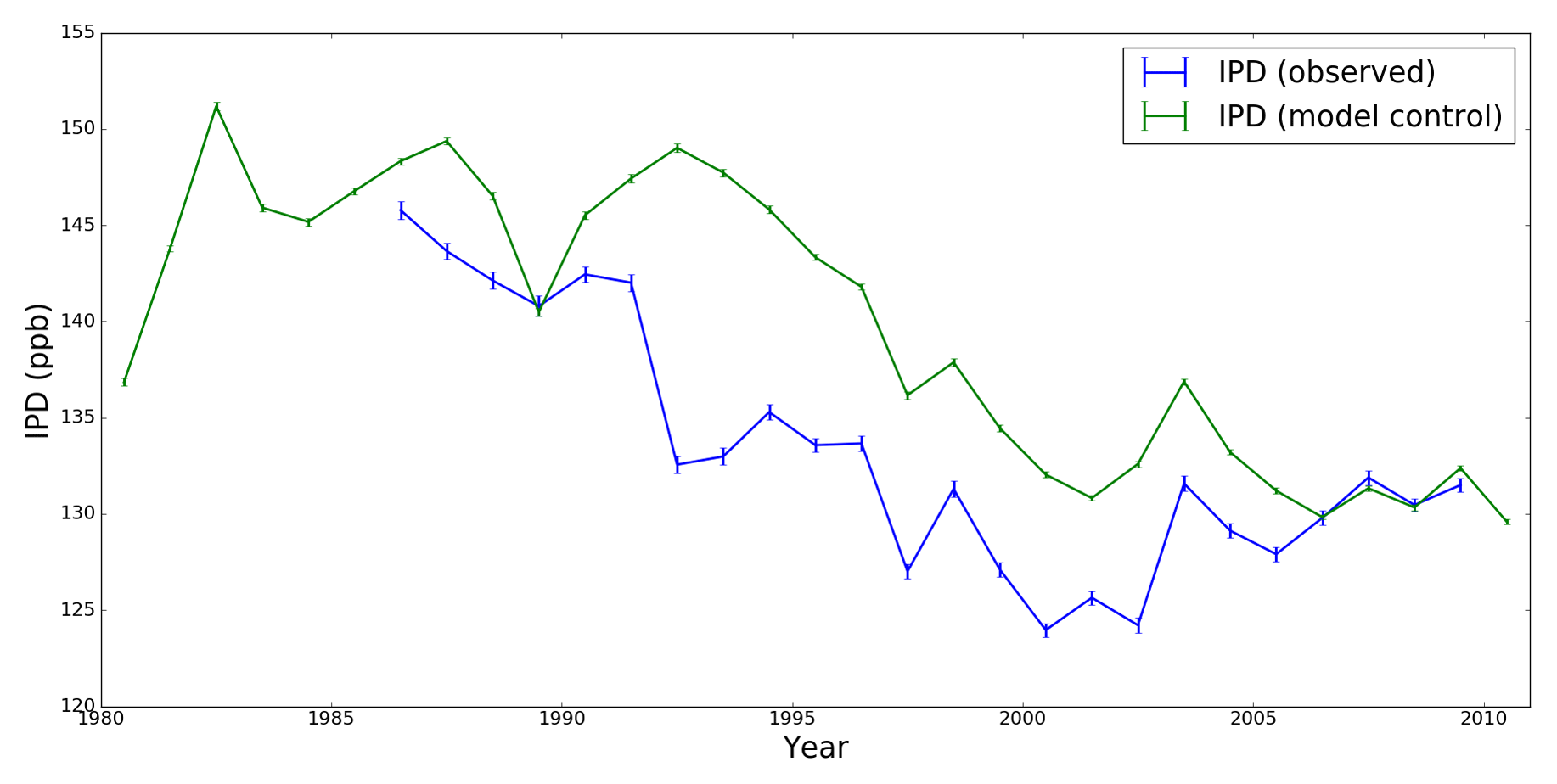
Figure 1Annual mean IPD values (ppb) determined by NOAA ESRL and TM5 model atmospheric CH4 mole fractions using data collected at seven geographical locations (Table 1). Vertical bars denote the 1 standard deviation associated with the annual mean.
The inter-polar difference (IPD) has been proposed as a sensitive indicator of changes in Arctic emissions that can be derived directly from network observations of atmospheric CH4 mole fraction. The IPD, as previously defined (Dlugokencky et al., 2003), is the difference between weighted annual means of CH4 mole fraction data collected at polar stations (those poleward of latitude) such as those from the NOAA Earth System Research Laboratory (ESRL) network (https://www.esrl.noaa.gov/gmd/dv/site/site_table2.php, last access: 10 December 2018). Data from individual sites are weighted inversely by the cosine of the station latitude and by the standard deviation of the data at a particular site. Dlugokencky et al. (2003) reported an abrupt drop in IPD during the early 1990s. They suggested this magnitude of change was indicative of a 10 Tg CH4 year−1 reduction, which they attribute to the collapse of fossil fuel production in Russia following the 1991 breakup of the Soviet Union (Dlugokencky et al., 2011). In more recent work, Dlugokencky et al. (2011) proposed that the IPD metric is potentially sensitive to changes in Arctic emissions as small as 3 Tg CH4 year−1, representing a value of 10 % of northern wetland emissions. However, studies have reported little or no increase in IPD between 1995 and 2010 (Fig. 1, Dlugokencky et al., 2003, 2011), a period during which rising Arctic temperatures were expected to lead to an increase in emissions (Mauritsen, 2016; McGuire et al., 2017). In this work, we examine how sensitive the IPD is to changing CH4 emissions by using model simulations guided by results from an analytical approach.
First, we derive the continuous version of the IPDC to introduce the atmospheric transport terms that are not considered in the subtraction approach. For our model, we have a local Arctic source (mass CH4 per unit time) and an isolated inter-polar source (mass CH4 per unit time) emitted at position r and time t. The IPDC is given by
where Δr is the graduation in latitude in the model and c(r,t) denotes atmospheric CH4 mole fraction (ppb) at latitude r and time t that includes influences from all other latitudes and previous times. The mole fraction can then be described as
where denotes the surface emission fluxes (g cm−2 s−1); denotes the fraction of emissions from location r′ at initial time t′ that contributes to the concentration at location r and a later time t, which includes atmospheric chemistry and transport; and (cm3 g−1) describes the conversion between emissions and atmospheric mole fraction (parts per billion, ppb) and takes the form , where Na and Mw denote Avogadro's constant (molecules mole−1) and the molar weight of CH4 (g mole−1), respectively, and ρ(r,t) denotes the number density of air (molec cm−3).
Our expression for IPDC can be reformulated as the difference between values determined at time t and a reference time t0. The reader is referred to Appendix A for a full derivation of the expressions used in this introduction. Equation (3) describes the IPD using the assumptions previously used (e.g. Dlugokencky et al., 2003): (1) the southern polar region contains no local sources, and (2) emissions from the northern polar region are too diffuse after transport between poles to significantly affect mole fractions at the southern polar region.
The first integral in Eq. (3) represents contributions from changes in northern polar sources between t and t0; and the second and third integral represent atmospheric transport terms that describe the contributions from intra-polar sources to the northern and southern polar mole fractions, respectively. To successfully isolate local Arctic emissions of CH4 using the IPD these atmospheric transport terms would have to cancel out. Taking into account that the characteristic timescale for inter-hemispheric transport of an air mass is ≃1 year (Holzer and Waugh, 2015) we argue that only a fortuitous set of circumstances would allow the IPD as previously defined to isolate local northern polar sources of CH4.
In the next section, we describe the data and methods used previously to define IPD, as well as the model calculations we use to explore the importance of these atmospheric transport terms, as illustrated in Eq. (3). In Sect. 3, we report the results from our numerical experiments. We conclude in Sect. 4.
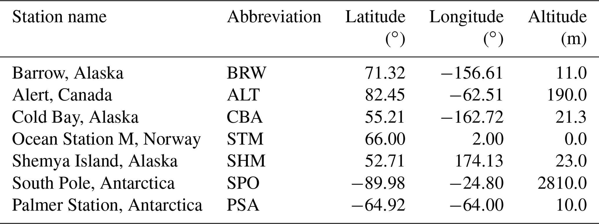
Table 1Details of the polar station used to calculate the IPD.
2.1 Observed and model IPD
To calculate the IPD, following Dlugokencky et al. (2011), we first group together a subset of NOAA ESRL global monitoring measurement sites that are located latitude (Table 1) and assign them as the north and south polar regions. For each polar region we calculate mean biweekly (measurements taken every 2 weeks) mole fractions across the stations, weighted inversely by station latitude and the standard deviation about the biweekly mean CH4 mole fraction. Biweekly values of IPD are then averaged over a calendar year to determine the annual IPD, which has been used in previous studies.
We use biweekly CH4 values determined from measurements of discrete air samples collected in flasks from the NOAA Cooperative Global Air Sampling Network (NOAA CGASN). Air samples (flasks) are collected at the sites and analysed for CH4 at NOAA ESRL in Boulder, Colorado, using a gas chromatograph with flame 220 ionization detection. Each sample aliquot is referenced to the WMO X2004 CH4 standard scale (Dlugokencky et al., 2005). Individual measurement uncertainties are calculated based on analytical repeatability and the uncertainty in propagating the WMO CH4 mole fraction standard scale. Analytical repeatability varies between 0.8 and 2.3 ppb and has a mean value of approximately 2 ppb averaged over the measurement record. Uncertainty in scale propagation is based on a comparison of discrete flask-air and continuous measurements at the MLO (Mauna Loa Observatory) and BRW observatories and has a fixed value 0.7 ppb. These two values are added in quadrature to estimate the total measurement uncertainty, equivalent to a ≃68 % confidence interval.
Five northern and two southern polar stations (Table 1) have data that cover the period discussed in previous studies (approximately 1986–2010) and a weekly resolution to calculate biweekly averages. We impute missing data filled using a two-stage approach. We use linear interpolation to replace missing measurements from a given week and year with the average of the measurement values from the same week of the three preceding and subsequent years (to provide a climatological value but preserve long-term trends in the data). If corresponding weekly measurements for the six neighbouring years are incomplete, we use a cubic spline interpolation. We calculate the uncertainties on the biweekly weighted concentration means from the polar regions using the formula for the standard error of a weighted mean μ (Taylor, 1997), , where the denominator represents weights assigned to each station i as a function of biweekly mole fraction standard deviation σi and the latitude ϕi of the station. We propagate these errors to determine the error on the annual IPD, following Dlugokencky et al. (2011).
We calculate the corresponding model IPD values by sampling TM5 (described below) at the time and location of each NOAA ESRL observation and processing the values as described above for the observations.
2.2 Numerical experiments
Building on the terms evaluated using our continuous IPDC model (Eq. 3) we use the TM5 atmospheric transport model (Krol et al., 2005) to (1) examine how perturbations in inter-polar emissions are transported to the polar regions and (2) determine the sensitivity of the IPD to different emission distributions.
For our numerical experiments, we run the TM5 model using a horizontal spatial resolution of 2∘ (latitude) and 3∘ (longitude), driven by meteorological fields from the European Centre for Medium-Range Weather Forecast (ECMWF) ERA-Interim reanalysis. Fossil fuel and agricultural emission estimates are taken from the EDGAR3.2 inventory (Olivier et al., 2005) with modifications (Schwietzke et al., 2016). Natural emissions are based on the prior values used by CarbonTracker-CH4 (Bergamaschi et al., 2005; Bruhwiler et al., 2014). Bruhwiler et al. (2014) reported posterior CH4 emission estimates for high northern latitudes that were 20 %–30 % smaller than prior values, which we use in our current experiments. An important consequence of our using these prior values is that the model IPD values have a positive bias compared to values determined by CH4 mole fraction measurements.
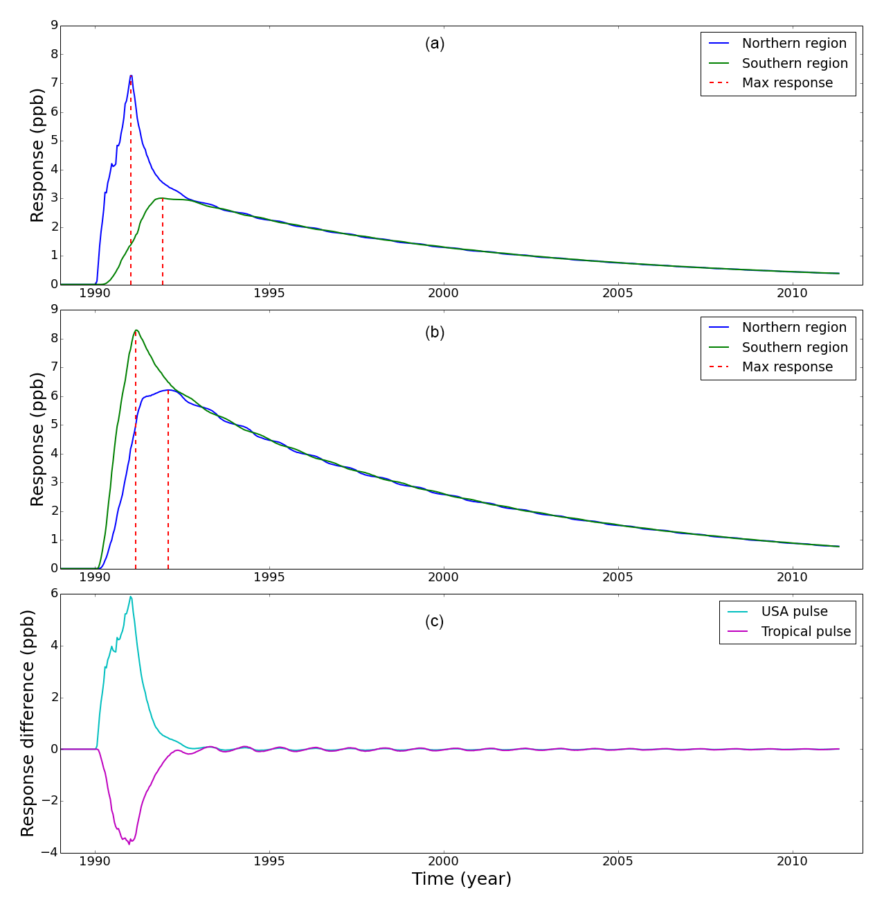
Figure 2The model response of atmospheric CH4 mole fraction sampled at northern and southern polar regions to a pulsed emission at (a) mid-latitude USA and (b) the tropics. Panel (c) shows the IPD response to these mid-latitude and tropical perturbations. In the interest of clarity, we omit error bars from the plots. Vertical red dashed lines denote the peak response time for each polar region.
We run a suite of targeted numerical experiments to test the sensitivity of the IPD to pulsed and noisy variations from mid-latitude and tropical emission sources. In practice, both sets of experiments integrate information from both atmospheric transport terms. We also consider experiments that included Arctic emissions with different constant growth rates and realistic variations in lower latitude emissions. As a control we use a simulation with constant emissions. Appendix B includes a presentation of the time series used to calculate the IPD from our experiments.
We initialize our TM5 numerical experiments from 1980 using initial conditions defined by the observed north–south distribution of CH4 in the early 1980s. Each experiment is run from 1980 to 2010, with mole fractions sampled at the time and location of the network observations.
2.2.1 Control run
Figure 1 shows that the model IPD for the control run is higher than observed values, as explained above. The model IPD also shows less variability than observed values. Variations of IPD in the early 1990s have been attributed to a rapid decline in fossil fuel production following the 1991 breakup of the Soviet Union (Dlugokencky et al., 2011). We determine the model response to changes in emissions (as described below) by subtracting the control run from the perturbed emissions runs.
2.2.2 Pulsed emission runs
To investigate the impact of a sustained continental-scale change in emissions on the weighted polar means and the IPD metric, we run the control experiment configuration but during the year 1990 we increase emissions by an amount that is evenly distributed throughout the year. In the first pulse experiment, we increase existing mid-latitude emissions over the contiguous USA by 10 Tg CH4. In the second experiment, we increase existing tropical land sources (within ) by 20 Tg CH4. We present polar mole fraction time series produced using the control and pulsed experiments shown in Appendix B.
2.2.3 Random noise emission runs
To investigate the role of intra- and inter-annual variations of emission sources on the IPD we rerun the two pulse experiments but superimpose standard uniform distribution noise 𝒰(0,1) on the emissions. We conduct two runs of TM5: one with a noise function of amplitude 10 Tg on US emissions and another with a function of amplitude 20 Tg on tropical sources. These experiments help us to determine the observability of changes in mid-latitude and tropical sources at the poles and whether the IPD can isolate local Arctic emission.
2.2.4 Arctic emission variation
To investigate the ability of IPD to detect a constant annual growth rate of Arctic emissions, we use the control experiment configuration but in three separate experiments we increase Arctic emission by 0.5 %, 1 %, and 2 % on an annual basis. Emissions are mostly limited to summer months (June–August) when the soil surface is typically not frozen.

Figure 3(a) Biweekly and annual model response of the IPD to changes in standard uniform distribution of random noise on prior mid-latitude USA and tropical emissions. (b) Annual mean response of IPD to constant growth of Arctic emissions. Vertical lines denote uncertainties on responses.
Figure 2 summarizes the results from our pulsed emission experiments. The model response at both poles to the 1990 pulse peaks rapidly and then falls off approximately exponentially over several years. The northern region tracer represents the sum of local Arctic emissions and the first atmospheric transport term in Eq. (3), and the southern region tracer represents the second atmospheric transport term in that equation.
Figure 2a shows that the mid-latitude pulse of 10 Tg CH4 results in a larger change at the northern polar stations (7.3 ppb peak) than at the southern polar stations (3.0 ppb peak). This reflects the longer transport time for the pulse to reach the southern stations during which time the pulse becomes more diffuse. More importantly, for the interpretation of the IPD we find that the northern polar stations experience the majority of the pulse 0.96 years before the southern polar stations. After 1991 the pulse responses decay with e-folding lifetimes of 4.43 and 8.94 years in the northern and southern polar stations, respectively. Figure 2c shows that the difference in pulse response at the poles decays from a maximum value in 1992 with an e-folding time of approximately 0.36 years.
Figure 2b shows that the peak of the 20 Tg CH4 tropical pulse reaches the southern polar region 0.92 years earlier than the northern polar region. This results in a larger change in southern polar CH4 mole fractions (8.3 ppb peak) compared to corresponding values over the northern polar regions. The earlier transit of the tropical pulse to the southern polar region reflects that much of the prior tropical CH4 fluxes that we perturb lie in the Southern Hemisphere. Responses to the tropical pulse decay after 1992 with e-folding lifetimes of 8.65 and 7.07 years for the northern and southern regions, respectively. The significant transport delay and disparity in responses means that an annual mean subtraction of northern and southern polar stations (IPD) will not remove the influence of the mid-latitude pulse and isolate local Arctic CH4 emissions as previously assumed.
Figure 3a shows that signal variations that we might expect from the atmospheric transport of intra- and inter-annual variation changes in emission sources can dominate the IPD signal. In response to noise superimposed on mid-latitude USA emissions, changes in biweekly IPD values have a mean value of 3.0 ppb (range −0.1–6.0 ppb). The corresponding changes in the annual IPD has a mean value of 3.0 ppb (range 0.3–5.4 ppb). The response of the biweekly IPD to noise on tropical emissions has a mean value of −2.8 ppb (range −12.8–5.6 ppb) and the corresponding response to the annual IPD has a mean value of −2.7 ppb (range −4.7–0.6 ppb). These experiments show that the IPD is susceptible to variations in inter-polar sources.
Table 2Number of years required to detect a statistically significant trend in Arctic emissions in the presence of inter-polar emission variations.
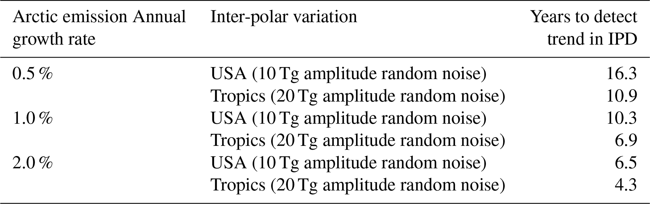
Figure 3b shows that IPD is sensitive to changes in local Arctic CH4 emissions, as expected, with a near-perfect correlation. We find only a modest response of IPD to large percentage increases in Arctic emissions: annual increases of 0.5 %, 1 %, and 2 % in Arctic emissions result in changes of 0.09, 0.17, and 0.35 ppb year−1 in IPD. IPD variations that might be expected from intra- and inter-annual variations in mid-latitude and tropical sources are typically much larger than the signal associated with changes in local Arctic emissions. We find that the IPD in the presence of a constant Arctic annual growth rate and intra- and inter-annual variations in mid-latitude and tropical emissions can detect a 0.5 % annual growth rate within 11–16 years to a 95 % confidence level (Weatherhead et al., 1998). Table 2 summarizes our results for different growth rates but generally the larger the Arctic growth rate the shorter it takes to detect the signal, as expected. The IPD is more susceptible to variations in northern mid-latitude sources than tropical sources, as described above. These results represent a best-case scenario for the IPD. In practice, there are also intra- and inter-annual variations associated with local Arctic emissions that will complicate the interpretation of the IPD and likely increase the time necessary to detect a statistically significant signal.
We critically assessed the inter-polar difference (IPD) as a robust metric for changes in Arctic emissions. The IPD has been previously defined as the difference between weighted means of atmospheric CH4 time series collected in the northern and southern polar regions. A continuous version of the IPDC model includes at least two additional terms associated with atmospheric transport. Using the TM5 atmospheric transport model we highlighted the importance of these atmospheric transport terms. We showed that IPD has a limited capacity to isolate changes in Arctic emissions.
We show that an inter-polar emission (here, we have evaluated emissions from mid-latitudes and the tropics) generally arrives at one pole earlier than the other pole by approximately 1 year, invalidating a key assumption of the IPD. We also show that a small amount of noise on prior mid-latitude or tropical sources that might be expected due to intra- and inter-annual source variations is not removed in the calculation of the IPD. While the IPD can detect a constant Arctic annual growth rate of emissions, any additional variation due to mid-latitude or tropical sources can delay detection of a statistically significant signal by up to 16 years.
Our study highlights the need for sustaining a spatially distributed and intercalibrated observation network for the early detection of changes in Arctic CH4 emissions. The ability to detect and quantify trends in these emissions directly from observations is attractive, but in reality we need to account for variations in extra-polar fluxes and differential atmospheric transport rates to the poles. This effectively demands the use of a model of atmospheric transport, which must be assessed using global distributed observations.
A Bayesian inference method that integrates information from prior knowledge and measurements is an ideal approach for quantifying changes in Arctic CH4 emissions, but assumes (a) reliable characterization of model error and (b) measurements that are sensitive to all major sources. Model error characterization is an ongoing process. Estimating CH4 emissions from atmospheric measurements is an undetermined (i.e. number of fluxes to be estimated ≫ number of observations available) and an ill-posed (i.e. several different solutions exist that are equally consistent with the available measurements) inverse problem. Prior emissions are required to regularize the inverse problem, allowing posterior fluxes to be determined that are consistent with prior knowledge and atmospheric CH4 measurements, as well as their respective uncertainties. Ground-based measurements represent invaluable information to determine atmospheric variations of CH4, but the spatial density of these data limits the resolution of corresponding posterior emission estimates to long temporal and large spatial scales. Column observations from satellites represent new, finer-scale information about atmospheric CH4, but they are generally less sensitive to surface processes than ground-based data. Daily global observations of atmospheric CH4 from the latest of these satellite instruments, TROPOMI aboard Sentinel-5P (launched in late 2017), promise to confront current understanding about Arctic emissions of CH4 described by land-surface models and bottom-up emission inventories. Passive satellite sensors, such as TROPOMI, rely on reflected sunlight so they are limited by cloudy scenes and by low-light conditions during boreal winter months. Active space-borne sensors (e.g. Methane Remote Sensing Lidar Mission, MERLIN, due for launch ≥ 2021) that employ onboard lasers to make measurements of atmospheric CH4 have the potential to provide useful observations day and night and throughout the year over the Arctic. The sensitivity of MERLIN to projected changes in Arctic emissions of CH4 is still to be determined. Another major challenge associated with satellite observations is cross-calibrating sensors to develop self-consistent time series that can be used to study trends over timescales longer than the expected lifetime of a satellite instrument (nominally <5 years). Even with access to all these data, it is clear that no simple, robust data metric exists without integrating the effects of atmospheric transport, but data-led analyses remain critical for underpinning knowledge of current and future changes in Arctic CH4 emissions.
Mole fraction data are available at https://www.esrl.noaa.gov/gmd/dv/site/site_table2.php (NOAA, 2018). The model data are available via the NOAA anonymous FTP site: ftp://aftp.cmdl.noaa.gov/user/lori/oscar/ipd (Bruhwiler, 2018).
Combining IPD(t) and c(t) described in Eqs. (1) and (2) results in two integral terms that underpin the continuous version of the IPD:
The first integral describes contributions to CH4 mole fractions in the Arctic region, including local emissions and atmospheric transport that originate outside the Arctic emitted at an earlier time t′. The second integral describes contributions to Antarctic CH4 mole fractions. Both terms are integrated over all previous times so they include the influence from older sources.
We now split the first integral into contributions from local Arctic emissions and those transported from sources outside the Arctic, and we split the Antarctic term in a similar way:
We assume that the Antarctic region (south of latitude ) contains no local sources so that mole fractions are determined exclusively by atmospheric transport. This eliminates the third term and reduces the integral limits in the second integral. We also assume that atmospheric transport of Arctic sources is too diffuse by the time they arrive at the Antarctic to contribute significantly to Antarctic mole fractions, i.e. for and . Using these assumptions (Eq. A2) now becomes
Equation (A3) includes three terms: (1) influence of local Arctic emissions on Arctic mole fractions; (2) an atmospheric transport term describing the influence of intra-polar sources (between latitudes and ) on Arctic mole fractions; and (3) an atmospheric transport term describing the influence of intra-polar sources (between latitudes and ) on Antarctic mole fractions.
If we now consider the change in IPD between some time t and a reference time t0 we can eliminate the need to integrate over all previous times, and instead we evaluate the integrals between t0 and t.
This can then be expressed as
In this final expression, the terms that describe local Arctic emissions and atmospheric transport are integrated between the current time t and some reference time. As a result, the emission term gives a measure of changes in Arctic emissions between t and t0.
For completeness, here we include the plots that complement the analysis reported in the main text. Figure B1 shows the model CH4 mole fraction corresponding to the weighted mean values at northern and southern polar region used to calculate the IPD in the control and pulsed experiments using the TM5. Figure B2 shows values of the annual mean IPD corresponding to our numerical experiments.

Figure B1TM5 model CH4 mole fractions (ppb) sampled at polar regions (Table 1) and weighted inversely by station latitude and standard deviation of the data at that site (see main text). (a) shows the response of a 10 Tg pulse over mid-latitude USA in 1990 over the northern and southern pole. (b) shows the response of a 20 Tg pulse over the tropics during 1990.
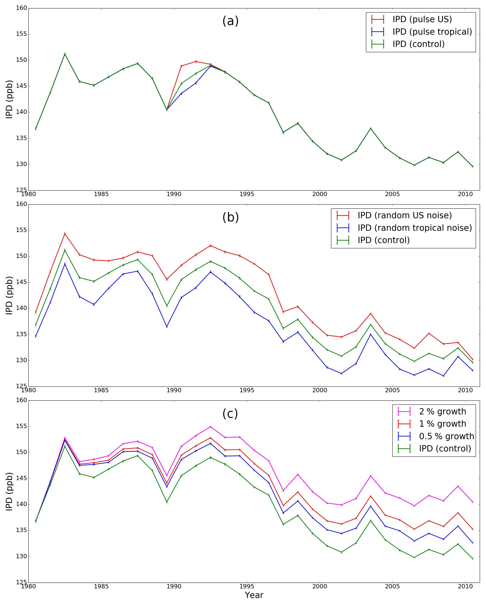
Figure B2The model IPD corresponding to the control and all the sensitivity experiments described in the main text.
OBDM and PIP co-led the mathematical derivation. TM5 model calculations were provided by LPB. Model analysis was led by OBD-M with contributions from LPB and PIP. PIP and OBDM co-wrote the paper with contributions from LPB.
The authors declare that they have no conflict of interest.
This article is part of the special issue “Greenhouse gAs Uk and Global Emissions (GAUGE) project (ACP/AMT inter-journal SI)”. It is not associated with a conference.
Oscar B. Dimdore-Miles was funded by a summer undergraduate project via the
NERC Greenhouse gAs Uk and Global Emissions (GAUGE) project (grant
NE/K002449/1). Paul I. Palmer gratefully acknowledges his Royal Society
Wolfson Research Merit Award. We thank NOAA/ESRL for the CH4 surface
mole fraction data which is provided by NOAA/ESRL PSD, Boulder, Colorado,
USA, from their website http://www.esrl.noaa.gov/psd/.
Edited by: Mathias Palm
Reviewed by: three
anonymous referees
AMAP: AMAP Assessment 2015: Methane as an Arctic climate forcer, Tech. rep., Arctic Monitoring and Assessment Programme (AMAP), Oslo, Norway, 2015. a, b
Bergamaschi, P., Krol, M., Dentener, F., Vermeulen, A., Meinhardt, F., Graul, R., Ramonet, M., Peters, W., and Dlugokencky, E. J.: Inverse modelling of national and European CH4 emissions using the atmospheric zoom model TM5, Atmos. Chem. Phys., 5, 2431–2460, https://doi.org/10.5194/acp-5-2431-2005, 2005. a
Bruhwiler, L.: NOAA, TM5 model runs in support of Dimdore-Miles et al., 2018, available at: ftp://aftp.cmdl.noaa.gov/user/lori/oscar/ipd, last access: 14 December 2018.
Bruhwiler, L., Dlugokencky, E., Masarie, K., Ishizawa, M., Andrews, A., Miller, J., Sweeney, C., Tans, P., and Worthy, D.: CarbonTracker-CH4: an assimilation system for estimating emissions of atmospheric methane, Atmos. Chem. Phys., 14, 8269–8293, https://doi.org/10.5194/acp-14-8269-2014, 2014. a, b
Christensen, T. R., Johansson, T., Åkerman, J., Mastepanov, M., Malmer, N., Friborg, T., Crill, P., and Svensson, B. H.: Thawing sub-arctic permafrost: Effects on vegetation and methane emissions, Geophys. Res. Lett., 31, L04501, https://doi.org/10.1029/2003GL018680, 2004. a
Dlugokencky, E., Houweling, S., Bruhwiler, L., Masarie, K., Lang, P., Miller, J., and Tansy, P. P.: Atmospheric methane levels off: Temporary pause or a new steady-state?, Geophys. Res. Lett., 30, 2058–2072, 2003. a, b, c, d
Dlugokencky, E., Nisbet, E., Fisher, R., and Lowry, D.: Global atmospheric methane: budget, changes and dangers, Philos. T. R. Soc., 369, 2058–2072, 2011. a, b, c, d, e, f
Dlugokencky, E. J., Myers, R. C., Lang, P. M., Masarie, K. A., Crotwell, A. M., Thoning, K. W., Hall, B. D., Elkins, J. W., and Steele, L. P.: Conversion of NOAA atmospheric dry air CH4 mole fractions to a gravimetrically prepared standard scale, J. Geophys. Res.-Atmos., 110, D18306, https://doi.org/10.1029/2005JD006035, 2005. a
Holzer, M. and Waugh, D. W.: Interhemispheric transit time distributions and path-dependent lifetimes constrained by measurements of SF6, CFCs, and CFC replacements, Geophys. Res. Lett., 42, 4581–4589, https://doi.org/10.1002/2015GL064172, 2015. a
Kirschke, S., Bousquet, P., Ciais, P., and Saunois, M.: Three decades of global methane sources and sinks, Nat. Geosci., 6, 813–823, 2013. a, b
Krol, M., Houweling, S., Bregman, B., van den Broek, M., Segers, A., van Velthoven, P., Peters, W., Dentener, F., and Bergamaschi, P.: The two-way nested global chemistry-transport zoom model TM5: algorithm and applications, Atmos. Chem. Phys., 5, 417–432, https://doi.org/10.5194/acp-5-417-2005, 2005. a
Mauritsen, T.: Greenhouse warming unleashed, Nat. Geosci., 9, 271–272, 2016. a
McGuire, A., Kelly, B., Guy, L. S., Wiggins, H., Bruhwiler, L., Frederick, J., Huntington, H., Jackson, R., Macdonald, R., Miller, C., Olefeldt, D., Schuur, E., and Turetsky, M.: Final Report: International Workshop to Reconcile Methane Budgets in the Northern Permafrost Region, Arctic Research Consortium of the United States (ARCUS), Fairbanks, Alaska, 14 pp., 2017. a
Nisbet, E., Dlugokencky, E., and Bousquet, P.: Methane on the Rise, Again, Science, 343, 493–494, 2014. a
NOAA: Observation sites of the NOAA Earth System Research Laboratory, Global Model Division, available at: https://www.esrl.noaa.gov/gmd/dv/site/site_table2.php, last access: 14 December 2018.
Olivier, J., Aardenne, J. V., Dentener, F., Pagliari, V., Ganzeveld, L., and Peters, J.: Recent trends in global greenhouse gas emissions:regional trends 1970–2000 and spatial distribution of key sources in 2000, Environm. Sci., 2, 81–99, 2005. a
Reagan, M. and Moridis, G.: Oceanic gas hydrate instability and dissociation under climate change scenarios, Geophys. Res. Lett., 34, 2283–2292, 2007. a
Rigby, M., Montzka, S., Prinn, R., White, J., Young, D., O'Doherty, S., Lunt, M., Ganesane, A., Manning, A., Simmonds, P., Salameh, P., Hart, C., Mühleg, J., Weiss, R., Fraser, P., Steele, L., Krummel, P., McCulloch, A., and Park, S.: Role of atmospheric oxidation in recent methane growth, P. Natl. Acad. Sci. USA, 114, 5373–5377, 2016. a
Saunois, M., Bousquet, P., Poulter, B., Peregon, A., Ciais, P., Canadell, J. G., Dlugokencky, E. J., Etiope, G., Bastviken, D., Houweling, S., Janssens-Maenhout, G., Tubiello, F. N., Castaldi, S., Jackson, R. B., Alexe, M., Arora, V. K., Beerling, D. J., Bergamaschi, P., Blake, D. R., Brailsford, G., Brovkin, V., Bruhwiler, L., Crevoisier, C., Crill, P., Covey, K., Curry, C., Frankenberg, C., Gedney, N., Höglund-Isaksson, L., Ishizawa, M., Ito, A., Joos, F., Kim, H.-S., Kleinen, T., Krummel, P., Lamarque, J.-F., Langenfelds, R., Locatelli, R., Machida, T., Maksyutov, S., McDonald, K. C., Marshall, J., Melton, J. R., Morino, I., Naik, V., O'Doherty, S., Parmentier, F.-J. W., Patra, P. K., Peng, C., Peng, S., Peters, G. P., Pison, I., Prigent, C., Prinn, R., Ramonet, M., Riley, W. J., Saito, M., Santini, M., Schroeder, R., Simpson, I. J., Spahni, R., Steele, P., Takizawa, A., Thornton, B. F., Tian, H., Tohjima, Y., Viovy, N., Voulgarakis, A., van Weele, M., van der Werf, G. R., Weiss, R., Wiedinmyer, C., Wilton, D. J., Wiltshire, A., Worthy, D., Wunch, D., Xu, X., Yoshida, Y., Zhang, B., Zhang, Z., and Zhu, Q.: The global methane budget 2000–2012, Earth Syst. Sci. Data, 8, 697–751, https://doi.org/10.5194/essd-8-697-2016, 2016. a, b
Schaefer, H., Fletcher, S. E. M., Veidt, C., Lassey, K. R., Brailsford, G. W., Bromley, T. M., Dlugokencky, E. J., Michel, S. E., Miller, J. B., Levin, I., Lowe, D. C., Martin, R. J., Vaughn, B. H., and White, J. W. C.: A 21st century shift from fossil-fuel to biogenic methane emissions indicated by 13CH4, Science, 352, 80–84, https://doi.org/10.1126/science.aad2705, 2016. a
Schuur, E. A. G., McGuire, A. D., Schadel, C., Grosse, G., Harden, J. W., Hayes, D. J., Hugelius, G., Koven, C. D., Kuhry, P., Lawrence, D. M., Natali, S. M., Olefeldt, D., Romanovsky, V. E., Schaefer, K., Turetsky, M. R., Treat, C. C., and Vonk, J. E.: Climate change and the permafrost carbon feedback, Nature, 520, 171–179, https://doi.org/10.1038/nature14338, 2015. a
Schwietzke, S., Sherwood, O. A., Bruhwiler, L. M. P., Miller, J. B., Etiope, G., Dlugokencky, E. J., Michel, S. E., Arling, V. A., Vaughn, B. H., White, J. W. C., and Tans, P. P.: Upward revision of global fossil fuel methane emissions based on isotope database, Nature, 538, 88–91, https://doi.org/10.1038/nature19797, 2016. a
Sweeney, C., Dlugokencky, E., Miller, C. E., Wofsy, S., Karion, A., Dinardo, S., Chang, R. Y.-W., Miller, J. B., Bruhwiler, L., Crotwell, A. M., Newberger, T., McKain, K., Stone, R. S., Wolter, S. E., Lang, P. E., and Tans, P.: No significant increase in long-term CH4 emissions on North Slope of Alaska despite significant increase in air temperature, Geophys. Res. Lett., 43, 6604–6611, https://doi.org/10.1002/2016GL069292, 2016. a
Tarnocai, C., Canadell, J. G., Schuur, E. A. G., Kuhry, P., Mazhitova, G., and Zimov, S.: Soil organic carbon pools in the northern circumpolar permafrost region, Global Biogeochem. Cy., 23, GB2023, https://doi.org/10.1029/2008GB003327, 2009. a
Taylor, J.: Introduction To Error Analysis: The Study of Uncertainties in Physical Measurements, University Science Books, 2nd edn., 1997. a
Turner, A., Frankenberg, C., Wennberg, P., and Jacob, D.: Ambiguity in the causes for decadal trends in atmospheric methane and hydroxyl, P. Natl. Acad. Sci. USA, 114, 5367–5372, 2016. a
Weatherhead, E. C., Reinsel, G. C., Tiao, G. C., Meng, X.-L., Choi, D., Cheang, W.-K., Keller, T., DeLuisi, J., Wuebbles, D. J., Kerr, J. B., Miller, A. J., Oltmans, S. J., and Frederick, J. E.: Factors affecting the detection of trends: Statistical considerations and applications to environmental data, J. Geophys. Res.-Atmos., 103, 17149–17161, 1998. a