Evaluation of autoconversion and accretion enhancement factors in general circulation model warm-rain parameterizations using ground-based measurements over the Azores

Wu, Peng; Xi, Baike; Dong, Xiquan; Zhang, Zhibo

doi:https://doi.org/10.5194/acp-18-17405-2018

Articles | Volume 18, issue 23

https://doi.org/10.5194/acp-18-17405-2018

Articles | Volume 18, issue 23

Research article

07 Dec 2018

Research article |

| 07 Dec 2018

Evaluation of autoconversion and accretion enhancement factors in general circulation model warm-rain parameterizations using ground-based measurements over the Azores

Peng Wu, Baike Xi, Xiquan Dong, and Zhibo Zhang

Abstract

A great challenge in climate modeling is how to parameterize subgrid cloud processes, such as autoconversion and accretion in warm-rain formation. In this study, we use ground-based observations and retrievals over the Azores to investigate the so-called enhancement factors, E_auto and E_accr, which are often used in climate models to account for the influence of subgrid variance of cloud and precipitation water on the autoconversion and accretion processes. E_auto and E_accr are computed for different equivalent model grid sizes. The calculated E_auto values increase from 1.96 (30 km) to 3.2 (180 km), and the calculated E_accr values increase from 1.53 (30 km) to 1.76 (180 km). Comparing the prescribed enhancement factors in Morrison and Gettleman (2008, MG08) to the observed ones, we found that a higher E_auto (3.2) at small grids and lower E_accr (1.07) are used in MG08, which might explain why most of the general circulation models (GCMs) produce too-frequent precipitation events but with too-light precipitation intensity. The ratios of the rain to cloud water mixing ratio (q_r/q_c) at E_accr=1.07 and E_accr=2.0 are 0.063 and 0.142, respectively, from observations, further suggesting that the prescribed value of E_accr=1.07 used in MG08 is too small to simulate precipitation intensity correctly. Both E_auto and E_accr increase when the boundary layer becomes less stable, and the values are larger in precipitating clouds (CLWP>75 gm⁻²) than those in non-precipitating clouds (CLWP<75 gm⁻²). Therefore, the selection of E_auto and E_accr values in GCMs should be regime- and resolution-dependent.

Download & links

Article (PDF, 2953 KB)

How to cite

How to cite.

Dates

Received: 18 May 2018 – Discussion started: 19 Jun 2018 – Revised: 21 Nov 2018 – Accepted: 24 Nov 2018 – Published: 07 Dec 2018

1 Introduction

Due to their vast areal coverage (Warren et al., 1986, 1988; Hahn and Warren, 2007) and strong radiative cooling effect (Hartmann et al., 1992; Chen et al., 2000), small changes in the coverage or thickness of marine boundary layer (MBL) clouds could change the radiative energy budget significantly (Hartmann and Short, 1980; Randall et al., 1984) or even offset the radiative effects produced by increasing greenhouse gases (Slingo, 1990). The lifetime of MBL clouds remains an issue in climate models (Yoo and Li, 2012; Jiang et al., 2012; Yoo et al., 2013; Stanfield et al., 2014) and represents one of the largest uncertainties in predicting future climate (Wielicki et al., 1995; Houghton et al., 2001; Bony and Dufresne, 2005).

MBL clouds frequently produce precipitation, mostly in the form of drizzle (Austin et al., 1995; Wood, 2005a, 2012; Leon et al., 2008). A significant amount of drizzle evaporates before reaching the surface, for example, about ∼76 % over the Azores region in the northeast Atlantic (Wu et al., 2015), which provides a water vapor source for MBL clouds. Due to their pristine environment and their proximity to the surface, MBL clouds and precipitation are especially sensitive to aerosol perturbations (Platnick and Twomey, 1994). Thus, accurate prediction of precipitation is essential in simulating the global energy budget and in constraining aerosol indirect effects in climate projections.

Due to the coarse spatial resolutions of the general circulation model (GCM) grid, many cloud processes cannot be adequately resolved and must be parameterized. For example, warm-rain parameterizations in most GCMs treat the condensed water as either clouds or rain from the collision–coalescence process that is partitioned into autoconversion and accretion subprocesses in model parameterizations (Kessler, 1969; Tripoli and Cotton, 1980; Beheng, 1994; Khairoutdinov and Kogan, 2000; Liu and Daum, 2004). Autoconversion represents the process of drizzle drops being formed through the self-collection of cloud droplets and accretion represents the process where raindrops grow by collecting cloud droplets. Autoconversion mainly accounts for precipitation initiation, while accretion primarily contributes to precipitation intensity. Autoconversion is often parameterized as functions of cloud droplet number concentration (N_c) and cloud water mixing ratio (q_c), while accretion depends on both cloud and rain water mixing ratios (q_c and q_r) (Kessler, 1969; Tripoli and Cotton, 1980; Beheng, 1994; Khairoutdinov and Kogan, 2000; Liu and Daum, 2004; Wood, 2005b). The majority of previous studies suggested that these two processes can be represented by power–law functions of cloud and precipitation properties (see Sect. 2 for details).

In conventional GCMs, the lack of information on the subgrid variance of clouds and precipitation leads to the unavoidable use of the grid-mean quantities ( $\overline{N_{c}}$ , $\overline{q_{c}}$ , and $\overline{q_{r}}$ , where the overbar henceforth denotes grid mean) in calculating autoconversion and accretion rates. MBL cloud liquid water path (CLWP) distributions are often positively skewed (Wood and Hartmann, 2006; Dong et al., 2014a, b); that is, the mean value is greater than the mode value. Thus, the mean value only represents a relatively small portion of samples. Also, due to the nonlinear nature of the relationships, the two processes depend significantly on the subgrid variability and co-variability of cloud and precipitation microphysical properties (Weber and Quass, 2012; Boutle et al., 2014). In some GCMs, subgrid-scale variability is often ignored or hard coded using constants to represent the variabilities under all meteorological conditions and across the entire globe (Pincus and Klein, 2000; Morrison and Gettleman, 2008; Lebsock et al., 2013). This could lead to systematic errors in precipitation rate simulations (Wood et al., 2002; Larson et al., 2011; Lebsock et al., 2013; Boutle et al., 2014; Song et al., 2018), where GCMs are found to produce too-frequent but too-light precipitation compared to observations (Zhang et al., 2002; Jess, 2010; Stephens et al., 2010; Nam and Quaas, 2012; Song et al., 2018). The bias is found to be smaller when using a probability density function (PDF) of cloud water to represent the subgrid-scale variability in autoconversion parameterization (Beheng, 1994; Zhang et al., 2002; Jess, 2010), or more complexly, by integrating the autoconversion rate over a joint PDF of liquid water potential temperature and total water mixing ratio (Cheng and Xu, 2009).

Process rate enhancement factors (E) are introduced when considering subgrid-scale variability in parameterizing grid-mean processes and they should be parameterized as functions of the PDFs of cloud and precipitation properties within a grid box (Morrison and Gettleman, 2008; Lebsock et al., 2013; Boutle et al., 2014). However, these values in some GCM parameterization schemes are prescribed as constants regardless of surface or meteorological conditions (Xie and Zhang, 2015). Boutle et al. (2014) used aircraft in situ measurements and remote sensing techniques to develop a parameterization for clouds and rain, in which they not only consider the subgrid variabilities under different grid scales but also consider the variation of cloud and rain fractions. The parameterization was found to reduce the precipitation estimation bias significantly. Hill et al. (2015) modified this parameterization and developed a regime- and cloud-type-dependent subgrid parameterization, which was implemented to the Met Office Unified Model by Walters et al. (2017), who found that the radiation bias is reduced when using the modified parameterization. Using ground-based observations and retrievals, Xie and Zhang (2015) proposed a scale-aware cloud inhomogeneity parameterization that they applied to the Community Earth System Model (CESM) and found that it can recognize spatial scales without manual tuning and can be applied to the entire globe. The inhomogeneity parameter is essential in calculating enhancement factors, since they affect the conversion rate from clouds to rain liquid. Xie and Zhang (2015), however, did not evaluate the validity of CESM simulations from their parameterization; the effect of N_c variability or the effect of covariance of clouds and rain on the accretion process was not assessed. Most recently, Zhang et al. (2018) derived the subgrid distribution of CLWP and N_c from the MODIS cloud product. They also studied the implication of subgrid cloud property variations for the simulation of autoconversion, in particular the enhancement factor, in GCMs. For the first time, the enhancement factor due to the subgrid variation of N_c was derived from satellite observation, and results reveal several regions downwind of biomass burning aerosols (e.g., Gulf of Guinea, east coast of South Africa), air pollution (i.e., East China Sea), and active volcanos (e.g., Kilauea in Hawaii and Ambae in Vanuatu) where the enhancement factor due to N_c is comparable or even larger than that due to CLWP. However, one limitation of Zhang et al. (2018) is the use of passive remote sensing data only, which cannot distinguish cloud and rain water.

Dong et al. (2014a, b) and Wu et al. (2015) reported MBL cloud and rain properties over the Azores and provided the possibility of calculating the enhancement factors using ground-based observations and retrievals. In this study, a joint retrieval method to estimate q_c and q_r profiles is proposed based on existing studies (Appendix A). Most of the calculations and analyses in this study are based on the Morrison and Gettelman (2008, MG08 hereafter) scheme. The enhancement factors in several other schemes are also discussed and compared with the observational results, and the approach in this study can be repeated for other microphysics schemes in GCMs. This paper is organized as follows: Sect. 2 includes a summary of the mathematical formulas from previous studies that can be used to calculate enhancement factors. Ground-based observations and retrievals are introduced in Sect. 3. Section 4 presents results and discussions, followed by a summary and conclusions in Sect. 5. The retrieval method used in this study is in Appendix A.

Table 1The parameters of autoconversion and accretion formulations for four parameterizations. NA – not available.

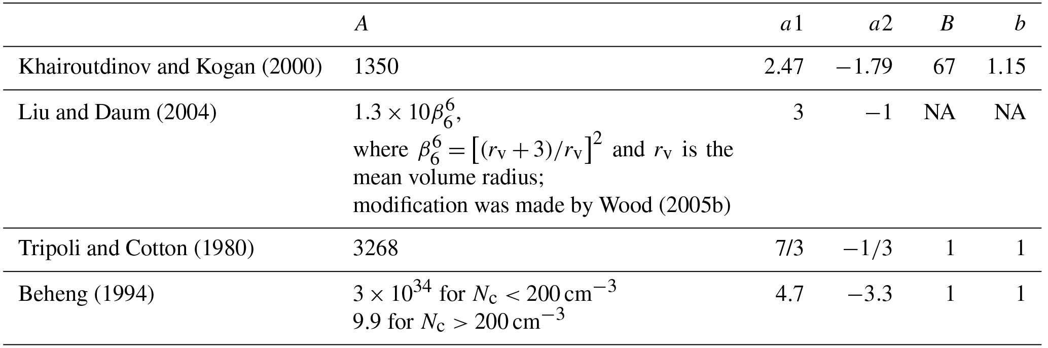
Download Print Version | Download XLSX

2 Mathematical background

Autoconversion and accretion rates in GCMs are usually parameterized as power–law equations (Tripoli and Cotton, 1980; Beheng, 1994; Khairoutdinov and Kogan, 2000; Liu and Daum, 2004):

\begin{matrix} (1) & {(\frac{\partial q_{r}}{\partial t})}_{auto} = A {\overline{q_{c}}}^{a 1} {\overline{N_{c}}}^{a 2}, \end{matrix}

\begin{matrix} (2) & {(\frac{\partial q_{r}}{\partial t})}_{accr} = B {(\overline{q_{c}} \overline{q_{r}})}^{b}, \end{matrix}

where A, a1, a2, B, and b are coefficients in different schemes listed in Table 1. $\overline{q_{c}}$ , $\overline{q_{r}}$ , and $\overline{N_{c}}$ are grid-mean cloud water mixing ratio, rain water mixing ratio, and droplet number concentration, respectively. Because it is widely used in model parameterizations, the detailed results from the Khairoutdinov and Kogan (2000) parameterization that has been used in the MG08 scheme will be shown in Sect. 4, while a summary will be given for other schemes.

Ideally, the covariance between physical quantities should be considered in the calculation of both processes. However, $\overline{q_{c}}$ and $\overline{N_{c}}$ in Eq. (1) are arguably not independently retrieved in our retrieval method, which will be introduced in this section and Appendix A. Thus, we only assess the individual roles of q_c and N_c subgrid variations in determining the autoconversion rate. q_c and q_r, on the other hand, are retrieved from two independent algorithms, as shown in Dong et al. (2014a, b), Wu et al. (2015), and Appendix A. The effect of the covariance of q_c and q_r on accretion rate will be assessed.

At the subgrid scale, the PDFs of q_c and N_c are assumed to follow a gamma distribution based on observational studies of optical depth in MBL clouds (Barker et al., 1996; Pincus et al., 1999; Wood and Hartmann, 2006):

\begin{matrix} (3) & P (x) = \frac{α^{ν}}{Γ (ν)} x^{ν - 1} e^{- α x}, \end{matrix}

where x represents q_c or N_c with grid-mean quantity $\overline{q_{c}}$ or $\overline{N_{c}}$ , represented by μ, $α = ν / μ$ is the scale parameter, σ² is the relative variance of x (= variance divided by μ²), and $ν = 1 / σ^{2}$ is the shape parameter. ν is an indicator of cloud field homogeneity, with large values representing homogeneous and small values indicating inhomogeneous cloud fields.

By integrating autoconversion rate, Eq. (1), over the grid-mean rate, Eq. (3), with respect to subgrid-scale variation of q_c and N_c, the autoconversion rate can be expressed as

\begin{matrix} (4) & {(\frac{\partial q_{r}}{\partial t})}_{auto} = A μ_{q_{c}}^{a 1} μ_{N_{c}}^{a 2} \frac{Γ (ν + a)}{Γ (ν) ν^{a}}, \end{matrix}

where a=a1 or a2. Comparing Eq. (4) to (1), the autoconversion enhancement factor (E_auto) can be given with respect to q_c and N_c:

\begin{matrix} (5) & E_{auto} = \frac{Γ (ν + a)}{Γ (ν) ν^{a}} . \end{matrix}

In addition to fitting the distributions of q_c and N_c, we also tried two other methods to calculate E_auto. The first is to integrate Eq. (1) over the actual PDFs from observed or retrieved parameters and the second is to fit a lognormal distribution for subgrid variability as has been done in other studies (e.g., Lebsock et al., 2013; Larson and Griffin, 2013). It is found that all three methods provide similar results. In this study, we use a gamma distribution that is consistent with MG08. Also, note that, in the calculation of E_auto from $\overline{N_{c}}$ , the negative exponent (−1.79) may cause singularity problems in Eq. (5). When this situation occurs, we perform direct calculations by integrating the PDF of $\overline{N_{c}}$ rather than using Eq. (5).

To account for the covariance of microphysical quantities in a model grid, it is difficult to apply a bivariate gamma distribution due to its complex nature. In this study, the bivariate lognormal distribution of q_c and q_r is used (Lebsock et al., 2013; Boutle et al., 2014) and can be written as

\begin{array}{l} P (\overline{q_{c}}, \overline{q_{r}}) = \frac{1}{2 π \overline{q_{c}} \overline{q_{r}} σ_{q_{c}} σ_{q_{r}} \sqrt{1 - ρ^{2}}} \exp \{- \frac{1}{2} \frac{1}{1 - ρ^{2}} \\ [{(\frac{\ln \overline{q_{c}} - μ_{q_{c}}}{σ_{q_{c}}})}^{2} - 2 ρ (\frac{\ln \overline{q_{c}} - μ_{q_{c}}}{σ_{q_{c}}}) (\frac{\ln \overline{q_{r}} - μ_{q_{r}}}{σ_{q_{r}}}) \\ (6) & + {(\frac{\ln \overline{q_{r}} - μ_{q_{r}}}{σ_{q_{r}}})}^{2}]\}, \end{array}

where σ is standard deviation and ρ is the correlation coefficient of q_c and q_r.

Similarly, by integrating the accretion rate in Eq. (2) from Eq. (6), we get the accretion enhancement factor (E_accr) of

\begin{array}{l} E_{accr} = {(1 + \frac{1}{ν_{q_{c}}})}^{\frac{{1.15}^{2} - 1.15}{2}} {(1 + \frac{1}{ν_{q_{r}}})}^{\frac{{1.15}^{2} - 1.15}{2}} \\ (7) & \exp (ρ {1.15}^{2} \sqrt{\ln (1 + \frac{1}{ν_{q_{c}}}) \ln (1 + \frac{1}{ν_{q_{r}}})}) . \end{array}

3 Ground-based observations and retrievals

The datasets used in this study were collected at the Department of Energy (DOE) Atmospheric Radiation Measurement (ARM) Mobile Facility (AMF), which was deployed on the northern coast of Graciosa Island (39.09^∘ N, 28.03^∘ W) from June 2009 to December 2010 (for more details, please refer to Rémillard et al., 2012, Dong et al., 2014a, and Wood et al., 2015). The detailed operational status of the remote sensing instruments at AMF is summarized in Fig. 1 of Rémillard et al. (2012) and discussed in Wood et al. (2015). The ARM Eastern North Atlantic (ENA) site was established on the same island in 2013 and provides long-term continuous observations.

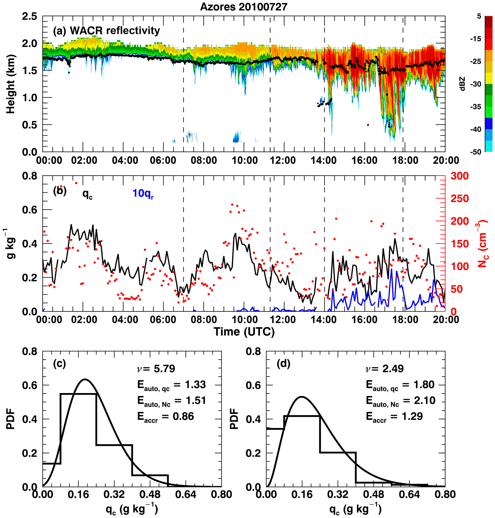
https://www.atmos-chem-phys.net/18/17405/2018/acp-18-17405-2018-f01

Figure 1Observations and retrievals over the Azores on 27 July 2010. (a) W-band ARM cloud radar (WACR) reflectivity (contour) superimposed with cloud-base height (black dots). (b) The black line represents averaged cloud water mixing ratio (q_c) within the top five range gates, the blue line represents averaged rain (×10) water mixing ratio within five range gates around maximum reflectivity, and red dots are the retrieved cloud droplet number concentration (N_c). Dashed lines represent two periods that have 60 km equivalent sizes with similar $\overline{q_{c}}$ but different distributions as shown by step lines in panels (c) and (d). Curved lines in panels (c) and (d) are fitted gamma distributions with the corresponding shape parameter (ν) shown on the upper right. N_c distributions are not shown. The calculated autoconversion (E_auto, qc from q_c and $E_{auto, N_{c}}$ from N_c) and accretion (E_accr) enhancement factors are also shown.

Download

The cloud-top heights (Z_top) were determined from the W-band ARM cloud radar (WACR) reflectivity and only single-layered and overcast low-level clouds with Z_top≤3 km were selected (the detailed selection criteria can be found in Dong et al., 2014a, b). Cloud-base heights (Z_base) were detected by a laser ceilometer (CEIL) and the cloud thickness was simply the difference between cloud-top and cloud-base heights. The cloud liquid water path (CLWP) was retrieved from microwave radiometer (MWR) brightness temperatures measured at 23.8 and 31.4 GHz using a statistical retrieval method with an uncertainty of 20 g m⁻² for CLWP<200 g m⁻² and 10 % for CLWP>200 g m⁻² (Liljegren et al., 2001; Dong et al., 2000). Precipitating status is identified through a combination of WACR reflectivity and Z_base. As in Wu et al. (2015), we labeled the status of a specific time as “precipitating” if the WACR reflectivity below the cloud base exceeded −37 dBZ. Note the differences of the reflectivity thresholds used here and in other studies. For example, these were −15 dBZ in Sauvageot and Omar (1987), −17 dBZ in Frisch et al. (1995), −19 to −16 dBZ in Wang and Geerts (2003), and −30 dBZ or lower in Kollias et al. (2011). The threshold used in this study is set at the cloud base rather than for the entire cloud layer as in the abovementioned studies. The −37 dBZ threshold is a statistical value from WACR observations over the Azores presented by Wu et al. (2015, Fig. 2a), in which it is found that using a higher threshold will miss a significant number of drizzling events, especially the clouds with virga.

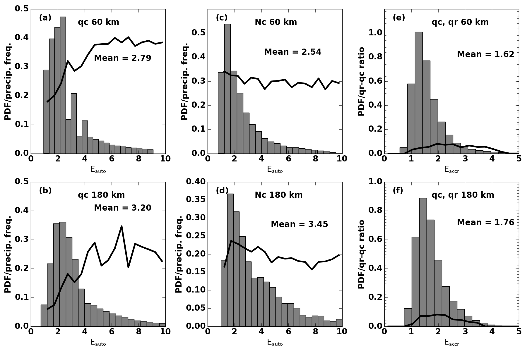
https://www.atmos-chem-phys.net/18/17405/2018/acp-18-17405-2018-f02

Figure 2Probability density functions (PDFs) of autoconversion (a–d) and accretion (e–f) enhancement factors calculated from q_c (a–b), N_c (c–d), and the covariance of q_c and q_r (e–f). The two rows show the results from 60 and 180 km equivalent sizes, respectively, with their average values. Black lines represent precipitation frequency in each bin in panels (a–d) and the ratio of layer-mean q_r to q_c in panels (e–f).

Download

The ARM merged sounding data have a 1 min temporal and 20 m vertical resolution below 3 km (Troyan, 2012). In this study, the merged sounding profiles are averaged to 5 min resolution. Pressure and temperature profiles are used to calculate air density (ρ_air) profiles and to infer adiabatic cloud water content.

Cloud droplet number concentration (N_c) is retrieved using the methods presented in Dong et al. (1998, 2014a, b) and is assumed to be constant with height. Vertical profiles of cloud and rain liquid water content (CLWC and RLWC) are retrieved by combining WACR reflectivity and CEIL attenuated backscatter, and by assuming adiabatic growth of cloud water. A detailed description is presented in Appendix A with the results from a selected case. The CLWC and RLWC values are transformed to q_c and q_r by dividing by air density (e.g., $q_{c} (z) = CLWC (z) / ρ_{air} (z))$ .

The estimated uncertainties for the retrieved q_c and q_r are 30 % and 18 %, respectively (see Appendix A). We used the estimated uncertainties of q_r and q_c as inputs of Eqs. (4) and (7) to assess the uncertainties of E_auto and E_accr. For instance, (1±0.3)q_c is used in Eq. (4) and the mean differences are then used as the uncertainty of E_auto. The same method is used to estimate the uncertainty for E_accr.

The autoconversion and accretion parameterizations dominate at different levels in a cloud layer. Autoconversion dominates around the cloud top, where drizzle drops form by the self-collection of cloud droplets, and accretion is dominant in the middle and lower parts of the cloud where raindrops grow by collecting cloud droplets. In accordance with the physical processes, we estimate autoconversion and accretion rates at different levels of a cloud layer in this study. The averaged q_c values within the top five range gates (∼215 m thick) are used to calculate E_auto. To calculate E_accr, we use the averaged q_c and q_r within five range gates around the maximum radar reflectivity. If the maximum radar reflectivity appears at the cloud base, then five range gates above the cloud base are used.

The ARM merged sounding data are also used to calculate lower tropospheric stability ( $LTS = θ_{700 hPa} - θ_{1000 hPa})$ , which is used to infer the boundary layer stability. In this study, unstable and stable boundary layers are defined as LTS less than 13.5 K and greater than 18 K, respectively, and an environment with an LTS between 13.5 and 18 K is defined as mid-stable (Wang et al., 2012; Bai et al., 2018). Enhancement factors in different boundary layers are summarized in Sect. 4.2 and may be used as reference for model simulations. Further, two regimes are classified: CLWP greater than 75 g m⁻² as precipitating and CLWP less than 75 g m⁻² as non-precipitating (Rémillard et al., 2012).

To evaluate the dependence of autoconversion and accretion rates on subgrid variabilities for different model spatial resolutions, an average wind speed within a cloud layer was extracted from merged sounding and used in sampling observations over certain periods to mimic different grid sizes in GCMs. For example, 2 h of observations correspond to a 72 km horizontal equivalent grid box if mean horizontal in-cloud wind speed is 10 m s⁻¹, and if the wind speed is 5 m s⁻¹, 4 h of observations are needed to mimic the same horizontal equivalent grid. We used six horizontal equivalent grid sizes (30, 60, 90, 120, 150, and 180 km) and mainly show the results from 60 and 180 km horizontal equivalent grid sizes in Sect. 4. For convenience, we use “equivalent size” to imply “horizontal equivalent grid size” from now on.

4 Results and discussions

In this section, we first show the data and methods using a selected case, followed by statistical analysis based on 19 months of data and multiple time intervals.

4.1 Case study

The selected case occurred on 27 July 2010 (Fig. 1a) over the Azores. This case was characterized by a long period of non-precipitating or light drizzling cloud development (00:00–14:00 UTC) before intense drizzle occurred (14:00–20:00 UTC). Wu et al. (2017) studied this case in detail to demonstrate the effect of wind shear on drizzle initiation. Here, we choose two periods corresponding to a 180 km equivalent size and having similar mean q_c near cloud top: 0.28 g kg⁻¹ for period c and 0.26 g kg⁻¹ for period d but with different distributions (Fig. 1c and d). The PDFs of q_c are then fitted using gamma distributions to get shape parameters (ν) as shown in Fig. 1c and d. Smaller ν is usually associated with a more inhomogeneous cloud field, which allows more rapid drizzle production and more efficient liquid transformation from cloud to rain (Xie and Zhang, 2015) in regions that satisfy precipitation criteria, which are usually controlled using a threshold q_r, droplet size, or relative humidity (Kessler, 1969; Liu and Daum, 2004). Period d has a wider q_c distribution than period c, resulting in a smaller ν and thus larger E_auto. Using the fitted ν, the E_auto from q_c calculated from Eq. (5) for period d is larger than that for period c (1.80 vs. 1.33). The E_auto values for periods d and c can also be calculated from N_c using the same procedure as q_c with a similar result (2.1 vs. 1.51). The E_accr values for periods d and c can be calculated from the covariance of q_c and q_r and Eq. (7). Not surprisingly, period d has larger E_accr than period c. The combination of larger E_auto and E_accr in period d contributes to rapid drizzle production and high rain rate as seen from WACR reflectivity and q_r in Fig. A1.

It is important to understand the physical meaning of enhancement factors in precipitation parameterization. For example, if we assume two scenarios for q_c with a model grid having the same mean values but different distributions, (1) the distribution is extremely homogeneous, and there is no subgrid variability because the cloud has the same chance to precipitate and the enhancement factors would be unity (this is true for arbitrary grid-mean q_c amount as well); and (2) the cloud field gets more and more inhomogeneous with a broad range of q_c within the model grid box, which results in a greater enhancement factor and increases the possibility of precipitation. That is, a large enhancement factor can make the part of the cloud with higher q_c within the grid box more efficient in generating precipitation, rather than the entire model grid.

Using the liquid water path (LWP) retrieved from the Moderate Resolution Imaging Spectroradiometer (MODIS) as an indicator of cloud inhomogeneity, Wood and Hartmann (2006) found that when clouds become more inhomogeneous, cloud fraction decreases, and open cells become dominant, accompanied by stronger drizzle (Comstock et al., 2007). The relationship between reduced homogeneity and stronger precipitation intensity found in this study is similar to the findings in other studies (e.g., Wood and Hartmann, 2006; Comstock et., 2007; Barker et al., 1996; Pincus et al., 1999).

It is clear that q_c and N_c in Fig. 1b are correlated with each other. In addition to their natural relationships, q_c and N_c in our retrieval method are also correlated (Dong et al., 2014a, b). Thus, the effect of q_c and N_c covariance on E_auto is not included in this study. In Fig. 1c and d, the results are calculated using an equivalent size of 180 km for the selected case on 27 July 2010. In Sect. 4.2, we will use these approaches to calculate their statistical results for multiple equivalent sizes using the 19-month ARM ground-based observations and retrievals.

4.2 Statistical result

For a specific equivalent size, e.g., 60 km, we estimate the shape parameter (ν) and calculate E_auto through Eqs. (5) and (7). The PDFs of E_auto for both 60 and 180 km equivalent sizes are shown in Fig. 2a–d. The distributions of E_auto values calculated from q_c with 60 and 180 km equivalent sizes (Fig. 2a and b) are different from each other (2.79 vs. 3.3). The calculated E_auto values range from 1 to 10, and most are less than 4. The average value for the 60 km equivalent size (2.79) is smaller than that for the 180 km equivalent size (3.2), indicating a possible dependence of E_auto on model grid size. Because drizzle-sized drops are primarily formed by autoconversion, we investigate the relationship between E_auto and precipitation frequency, which is defined as the average percentage of drizzling occurrence based on radar reflectivity below cloud base. Given the average LWP over the Azores from Dong et al. (2014b, 109–140 g m⁻²), the precipitation frequency (black lines in Fig. 2a and b) agrees well with those from Kubar et al. (2009, 0.1–0.7 from their Fig. 11). The precipitation frequency within each bin shows an increasing trend for E_auto from 0 to 4–6, then oscillates when E_auto>6, indicating that in the precipitation initiation process, E_auto keeps increasing to a certain value (∼6) until the precipitation frequency reaches a near-steady state. Higher precipitation frequency does not necessarily result in larger E_auto values but instead may produce more drizzle-sized drops from autoconversion process when the cloud is precipitating.

The PDFs of E_auto calculated from N_c also share similar patterns of positive skewness and peaks at ∼1.5–2.0 for the 60 and 180 km equivalent sizes (Fig. 2c and d). Although the average values are close to their q_c counterparts (2.54 vs. 2.79 for 60 km and 3.45 vs. 3.2 for 180 km), the difference in E_auto between 60 and 180 km equivalent sizes becomes large. The precipitation frequencies within each bin are nearly constant or decrease slightly, which is different from their q_c counterparts shown in Fig. 2a and b. This suggests complicated effects of droplet number concentration on precipitation initiation and warrants more exploration of aerosol–cloud–precipitation interactions. As mentioned in Sect. 2, q_c and N_c are also fitted using lognormal distributions to calculate E_auto. The results are close to those in Fig. 2 (not shown here), with average values of 3.28 and 3.84, respectively, for 60 and 180 km equivalent sizes. Because the E_auto values calculated from q_c and N_c are close to each other, we will focus on analyzing the results from q_c only for simplicity and clarity. The effect of q_c and N_c covariance, as stated in Sect. 4.1, is not presented in this study due to the intrinsic correlation in the retrieval (Dong et al., 2014a, b, and Appendix A of this study).

The covariance of q_c and q_r is included in calculating E_accr and the results are shown in Fig. 2e and f. The calculated E_accr values range from 1 to 4, with mean values of 1.62 and 1.76 for 60 and 180 km equivalent sizes, respectively. These two mean values are much greater than the prescribed value used in MG08 (1.07). Since accretion is dominant in the middle and lower parts of the cloud where raindrops sediment and continue to grow by collecting cloud droplets, we superimpose the ratio of q_r to q_c within each bin (black lines in Fig. 2e and f) to represent the portion of rain water in the cloud layer. In both panels, the ratios are less than 15 %, which means that q_r can be 1 order of magnitude smaller than q_c. The differences in magnitude are consistent with previous CloudSat and aircraft results (e.g., Boutle et al., 2014). This ratio increases from E_accr=0 to ∼2 and then decreases, suggesting that the conversion efficiency cannot be infinitely increased with E_accr under available cloud water. The ratio of q_r to q_c increases from E_accr=1.07 (0.063) to E_accr=2.0 (0.142), indicating that the fraction of rain water in total liquid water using the prescribed E_accr is too low. This ratio could be increased significantly using a large E_accr value, therefore increasing precipitation intensity in the models. This further suggests that the prescribed value of E_accr=1.07 used in MG08 is too small to correctly simulate precipitation intensity in the models. Therefore, similar to the conclusions in Lebsock et al. (2013) and Boutle et al. (2014), we suggest increasing E_accr from 1.07 to 1.5–2.0 in GCMs.

To illustrate the impact of using prescribed enhancement factors, autoconversion and accretion rates are calculated using the prescribed values (e.g., 3.2 for E_auto and 1.07 for E_accr, MG08; Xie and Zhang, 2015) and the newly calculated ones in Fig. 2 that use observations and retrievals. Figure 3 shows the joint density of autoconversion (Fig. 3a and b) and accretion rates (Fig. 3c and d) from observations (x axis) and model parameterizations (y axis) for 60 and 180 km equivalent sizes. Despite the spread, the peaks in the joint density of autoconversion rate appear slightly above the 1:1 line, especially for the 60 km equivalent size, suggesting that cloud droplets in the model are more easily converted into drizzle/raindrops than in the observations. On the other hand, the peaks in the accretion rate appear slightly below the 1:1 line, which indicates that simulated precipitation intensities are lower than observed ones. The magnitudes of the two rates are consistent with Khairoutdinov and Kogan (2000), Liu and Daum (2004), and Wood (2005b).

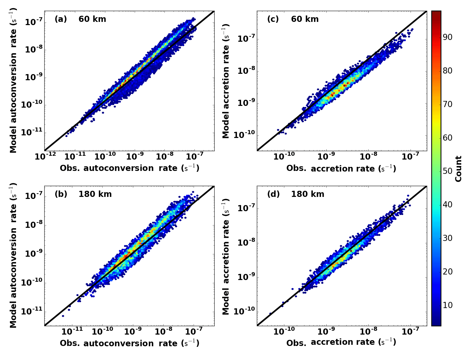
https://www.atmos-chem-phys.net/18/17405/2018/acp-18-17405-2018-f03

Figure 3Comparison of autoconversion (a–b) and accretion (c–d) rates derived from observations (x axis) and from the model (y axis). Results are for 60 km (a, c) and 180 km (b, d) model equivalent sizes. Colored dots represent joint number densities.

Download

Compared to the observations, the precipitation in GCMs occurs at higher frequencies with lower intensities, which might explain why the total precipitation amounts are close to surface measurements over an entire grid box. This “promising” result, however, fails to simulate precipitation on the right scale and cannot capture the correct rain water amount, thus providing limited information in estimating rain water evaporation and air–sea energy exchange.

Clouds in an unstable boundary layer have a better chance of getting moisture supply from the surface by upward motion than clouds in a stable boundary layer. Precipitation frequencies are thus different in these two boundary layer regimes. For example, clouds in a relatively unstable boundary layer produce drizzle more easily than those in a stable boundary layer. Given the same boundary layer conditions, CLWP is an important factor in determining the precipitation status of clouds. Over the Azores, precipitating clouds are more likely to have CLWP greater than 75 g m⁻² than their non-precipitating counterparts (Rémillard et al., 2012). To further investigate what conditions and parameters can significantly influence the enhancement factors, we classify low-level clouds according to their boundary layer conditions and CLWPs.

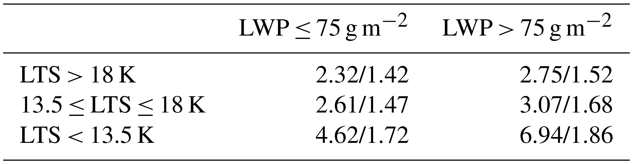
The averaged E_auto and E_accr values for each category are listed in Table 2. Both E_auto and E_accr increase when the boundary layer becomes less stable, and these values become larger in precipitating clouds (CLWP>75 g m⁻²) than those in non-precipitating clouds (CLWP<75 g m⁻²). In model parameterizations, the autoconversion process only occurs when q_c or cloud droplet size reaches a certain threshold (e.g., Kessler, 1969; Liu and Daum, 2004). Thus, it will not affect model simulations if a valid E_auto is assigned to Eq. (1) in a non-precipitating cloud. The E_auto values in both stable and mid-stable boundary layer conditions are smaller than the prescribed value of 3.2, while the values in unstable boundary layers are significantly larger than 3.2, regardless of whether they are precipitating. All E_accr values are greater than the constant of 1.07. The E_auto values in Table 2 range from 2.32 to 6.94 and the E_accr values vary from 1.42 to 1.86, depending on different boundary layer conditions and CLWPs. Therefore, as suggested by Hill et al. (2015), the selection of E_auto and E_accr values in GCMs should be regime-dependent.

Table 2Autoconversion (left values) and accretion (right values) enhancement factors in different boundary layer conditions (LTS>18 K for stable, LTS<13.5 K for unstable, and LTS within 13.5 and 18 K for mid-stable) and in different LWP regimes (LWP≤75 g m⁻² for non-precipitating and LWP>75 g m⁻² for precipitating).

Download Print Version | Download XLSX

To properly parameterize subgrid variabilities, the approaches of Hill et al. (2015) and Walters et al. (2017) can be adopted. To use MG08 and other parameterizations in GCMs as listed in Table 1, proper adjustments can be made according to the model grid size, boundary layer conditions, and precipitating status. As stated in the methodology, we used a variety of equivalent sizes. Figure 4 demonstrates the dependence of both enhancement factors on different model grid sizes. The E_auto values (red line) increase from 1.97 at an equivalent size of 30 km to 3.15 at an equivalent size of 120 km, which are 38.4 % and 2 % percent lower than the prescribed value (3.2, upper dashed line). After that, the E_auto values remain relatively constant at ∼3.18 when the equivalent model size is 180 km, which is close to the prescribed value of 3.2 used in MG08. This result indicates that the prescribed value in MG08 is appropriate for large grid sizes in GCMs. The E_accr values (blue line) increase from 1.53 at an equivalent size of 30 km to 1.76 at an equivalent size of 180 km, increases of 43 % and 64 %, respectively, larger than the prescribed value (1.07, lower dashed line). The shaded areas represent the uncertainties in E_auto and E_accr associated with the uncertainties in the retrieved q_c and q_r. When equivalent size increases, the uncertainties decrease slightly. The prescribed E_auto is close to the upper boundary of uncertainties except for the 30 km equivalent size, while the prescribed E_accr is significantly lower than the lower boundary.

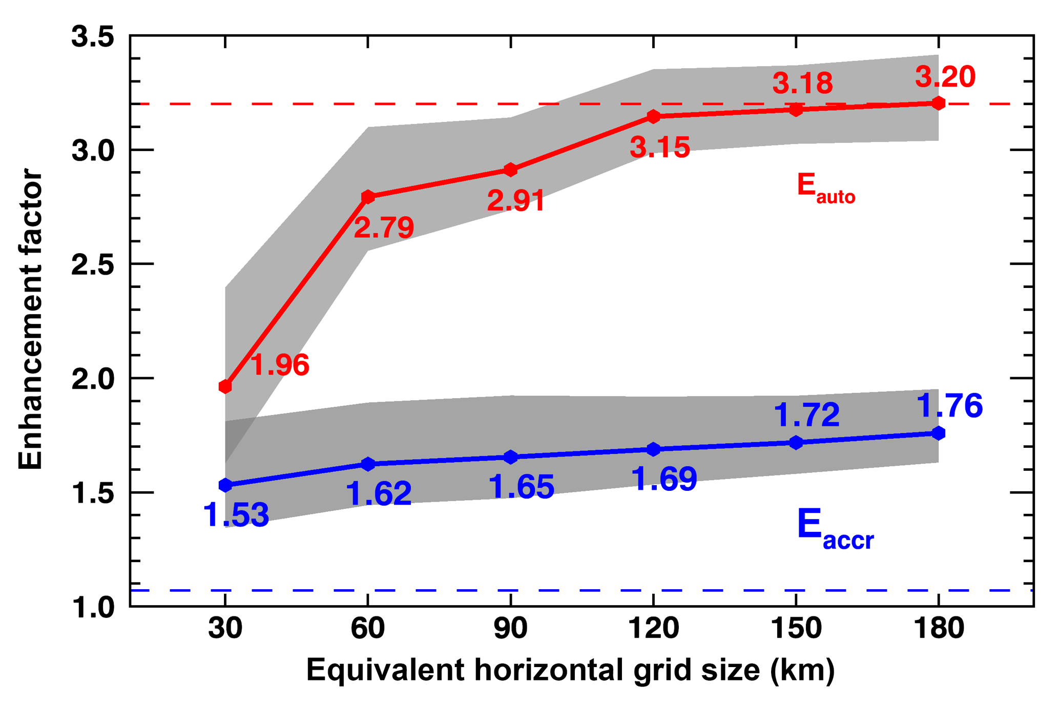
https://www.atmos-chem-phys.net/18/17405/2018/acp-18-17405-2018-f04

Figure 4Autoconversion (red line) and accretion (blue line) enhancement factors as a function of equivalent sizes. The shaded areas are calculated by varying q_c and q_r within their retrieval uncertainties. The two dashed lines show the constant values of autoconversion (3.2) and accretion (1.07) enhancement factors prescribed in MG08.

Download

It is noted that E_auto and E_accr depart from their prescribed values in opposite directions as the equivalent size increases. For models with finer resolutions (e.g., 30 km), both E_auto and E_accr are significantly different from the prescribed values, which can partially explain the issue of “too-frequent” and “too-light” precipitation. Under both conditions, the accuracy of precipitation estimation is degraded. For models with coarser resolutions (e.g., 180 km), the average E_auto is exactly 3.2, while E_accr is much larger than 1.07 when compared to finer-resolution simulations. In such situations, the simulated precipitation will be dominated by the too-light problem, in addition to being regime-dependent (Table 2), and as in Xie and Zhang (2015), E_auto and E_accr should also be scale-dependent.

Also note that the location of ground-based observations and retrievals used in this study is in the remote ocean, where the MBL clouds mainly form in a relatively stable boundary layer and are characterized by high precipitation frequency. Even in such environments, however, GCMs overestimate the precipitation frequency (Ahlgrimm and Forbes, 2014).

To further investigate how enhancement factors affect precipitation simulations, we use E_auto as a fixed value of 3.2 in Eq. (4) and then calculate the q_c needed for models to reach the same autoconversion rate as observations. The q_c differences between models and observations are then calculated, which represent the q_c adjustment in models to achieve a realistic autoconversion rate in the simulations. Similar to Fig. 1, the PDFs of q_c differences (model–observation) are plotted in Fig. 5a and b for 60 and 180 km equivalent sizes. Figure 5c shows the average percentages of model q_c adjustments for different equivalent sizes. The mode and average values for the 30 km equivalent size are negative, suggesting that models need to simulate lower q_c in general to get reasonable autoconversion rates. Lower q_c values are usually associated with smaller E_auto values that induce lower simulated precipitation frequency. On average, the percentage of q_c adjustments decreases with increasing equivalent size. For example, the adjustments for finer resolutions (e.g., 30–60 km) can be ∼20 % of the q_c, whereas adjustments in coarse-resolution models (e.g., 120–180 km) are relatively small because the prescribed E_auto (equal to 3.2) is close to the observed ones (Fig. 4), and when equivalent size is 180 km, no adjustment is needed. The adjustment method presented in Fig. 5, however, may change cloud water substantially and may cause a variety of subsequent issues, such as altering cloud radiative effects and disrupting the hydrological cycle. The assessment in Fig. 5 only provides a reference to the equivalent effect on cloud water by using the prescribed E_auto value as compared to those from observations.

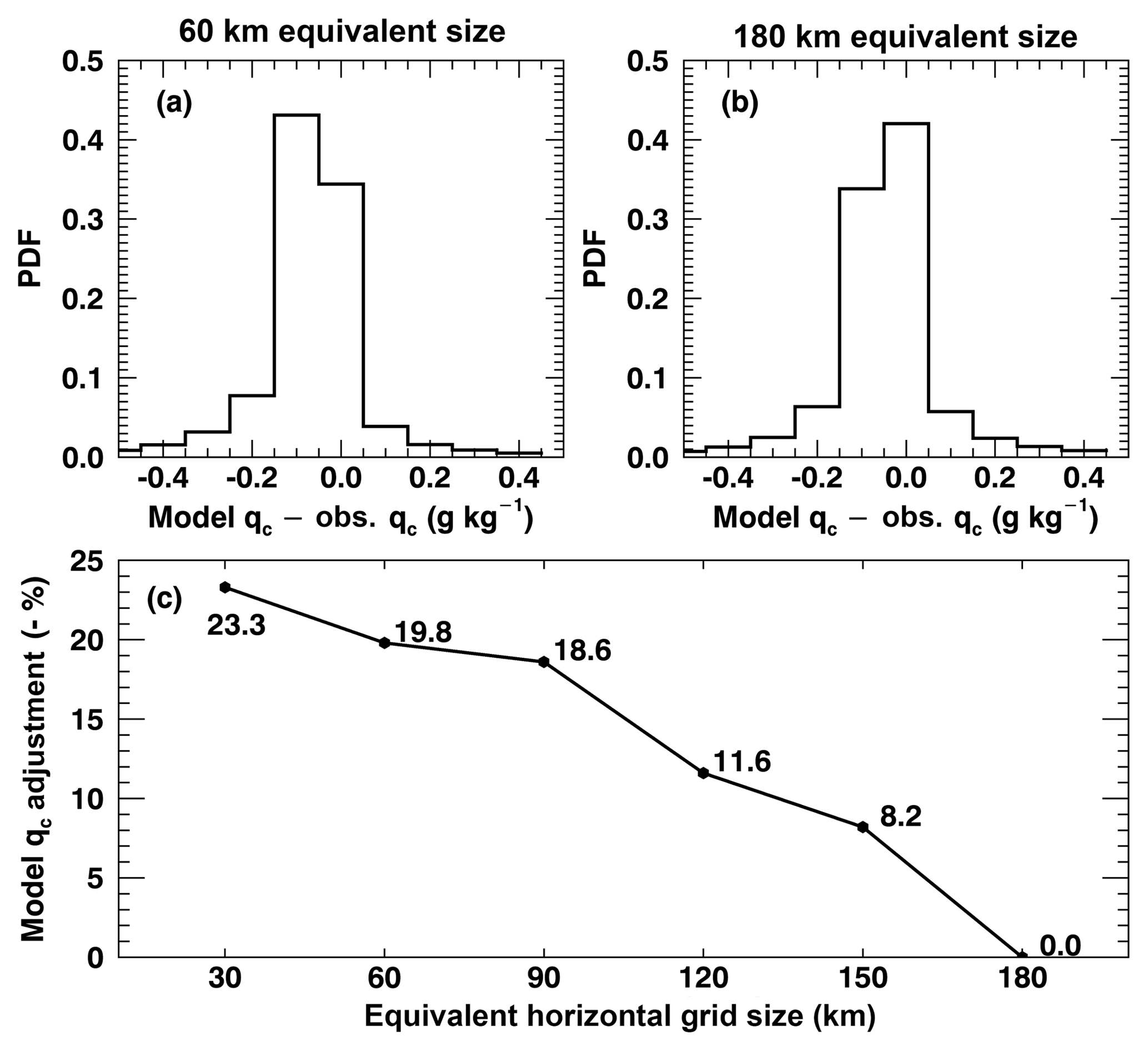
https://www.atmos-chem-phys.net/18/17405/2018/acp-18-17405-2018-f05

Figure 5q_c needed for models to adjust to reach the same autoconversion rate as observations for (a) 60 km and (b) 180 km model equivalent sizes. Positive biases represent increased q_c required in models, and negative biases mean decreased q_c. The average percentages of adjustments for different equivalent sizes are shown in panel (c). Note that the percentages in the vertical axis are negative.

Download

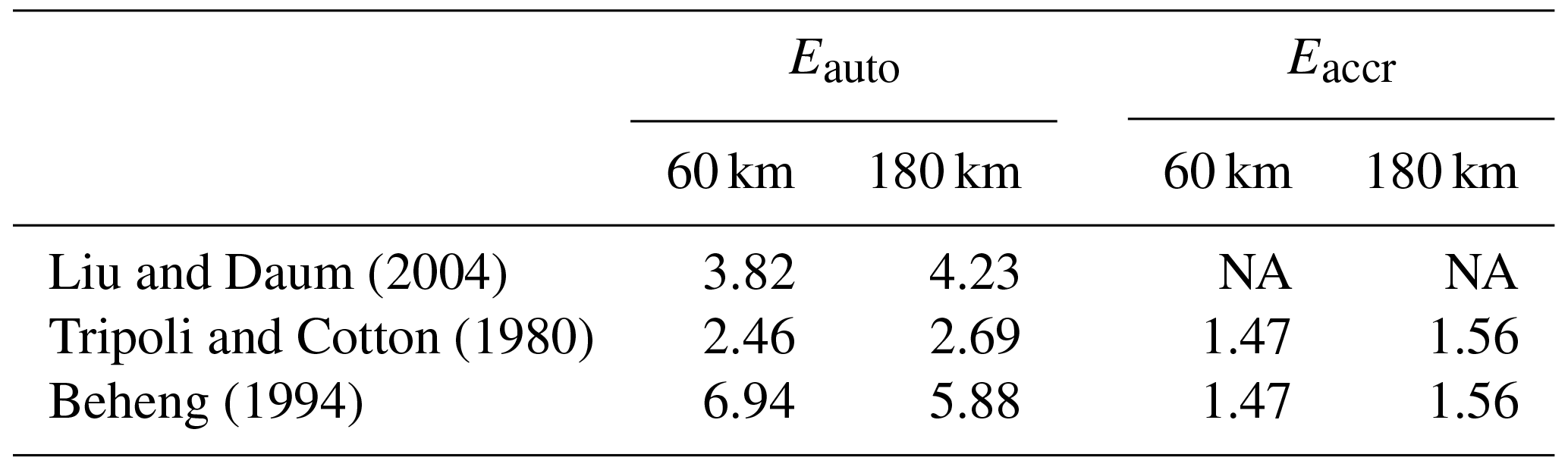
All above discussions are based on the prescribed E_auto and E_accr values (3.2 and 1.07) in MG08, whereas there are quite a few parameterizations that have been published so far. In this study, we list E_auto and E_accr for three other widely used parameterization schemes in Table 3, which are given only for 60 and 180 km equivalent sizes. The values of the exponent in each scheme directly affect the values of the enhancement factors. For example, the scheme in Beheng (1994) has the highest degree of nonlinearity and hence the largest enhancement factors. The scheme in Liu and Daum (2004) is very similar to the scheme in Khairoutdinov and Kogan (2000) because both schemes have a physically realistic dependence on cloud water content and number concentration (Wood, 2005b). For a detailed overview and discussion of various existing parameterizations, please refer to Liu and Daum (2004), Liu et al. (2006a), Liu et al. (2006b), Wood (2005b), and Michibata and Takemura (2015). A physical-based autoconversion parameterization was developed by Lee and Baik (2017), in which the scheme was derived by solving the stochastic collection equation with an approximated collection kernel that is constructed using the terminal velocity of cloud droplets and the collision efficiency obtained from a particle trajectory model. Due to the greatly increased complexity of their equation, we do not attempt to calculate E_auto here but it should be examined in future studies due to the physically appealing Lee and Baik (2017) scheme.

5 Summary

To better understand the influence of subgrid cloud variations on the warm-rain process simulations in GCMs, we investigated the warm-rain parameterizations of autoconversion (E_auto) and accretion (E_accr) enhancement factors in MG08. These two factors represent the effects of subgrid cloud and precipitation variabilities when parameterizing autoconversion and accretion rates as functions of grid-mean quantities. E_auto and E_accr are prescribed as 3.2 and 1.07, respectively, in the widely used MG08 scheme. To assess the dependence of the two parameters on subgrid-scale variabilities, we used ground-based observations and retrievals collected at the DOE ARM Azores site to reconstruct the two enhancement factors in different equivalent sizes.

Table 3Autoconversion and accretion enhancement factors (E_auto and E_accr) for the parameterizations in Table 1, except for the Khairoutdinov and Kogan (2000) scheme. The values are averaged for 60 and 180 km equivalent sizes. NA – not available.

Download Print Version | Download XLSX

From the retrieved q_c and q_r profiles, the averaged q_c values within the top five range gates are used to calculate E_auto, and the averaged q_c and q_r within five range gates around maximum reflectivity are used to calculate E_accr. The calculated E_auto values from observations and retrievals increase from 1.96 at an equivalent size of 30 km to 3.18 at an equivalent size of 150 km. These values are 38 % and 0.625 % lower than the prescribed value of 3.2. The prescribed value in MG08 represents well the large grid sizes in GCMs (e.g., 180² km² grid). On the other hand, the E_accr values increase from 1.53 at an equivalent size of 30 km to 1.76 at an equivalent size of 180 km, which are 43 % and 64 % higher than the prescribed value (1.07). The higher E_auto and lower E_accr prescribed in GCMs help to explain the issue of too-frequent precipitation events with too-light precipitation intensity. The ratios of rain to cloud liquid water increase with increasing E_accr from 0 to 2 and then decrease thereafter; the values at E_accr=1.07 and E_accr=2.0 are 0.063 and 0.142, further underscoring that the prescribed value of E_accr=1.07 is too small to simulate correct precipitation intensity in models.

To further investigate what conditions and parameters can significantly influence the enhancement factors, we classified low-level clouds according to their boundary layer conditions and CLWPs. Both E_auto and E_accr increase when the boundary layer conditions become less stable, and the values are larger in precipitating clouds (CLWP>75 g m⁻²) than those in non-precipitating clouds (CLWP<75 g m⁻²). The E_auto values in both stable and mid-stable boundary layer conditions are smaller than the prescribed value of 3.2, while those in unstable boundary layer conditions are significantly larger than 3.2 regardless of whether or not the cloud is precipitating (Table 2). All E_accr values are greater than the prescribed value of 1.07. Therefore, the selection of E_auto and E_accr values in GCMs should be regime-dependent, which also has been suggested by Hill et al. (2015) and Walters et al. (2017).

This study, however, did not include the effect of uncertainties in GCM simulated cloud and precipitation properties on subgrid-scale variations. For example, we did not consider the behavior of the two enhancement factors under different aerosol regimes, a condition which may affect the precipitation formation process. The effect of aerosol–cloud–precipitation interactions on cloud and precipitation subgrid variabilities may be of comparable importance to meteorological regimes and precipitation status and deserves further study. Other than the large-scale dynamics, e.g., LTS in this study, upward/downward motion at subgrid scale may also modify cloud and precipitation development and affect the calculations of enhancement factors. The investigation of the dependence of E_auto and E_accr on aerosol type and concentration as well as on vertical velocity would be a natural extension and complement the current study. In addition, other factors may also affect precipitation frequency and intensity even under the same aerosol regimes and even if the clouds have similar cloud water content. Wind shear, for example, as presented in Wu et al. (2017), is an external variable that can affect precipitation formation. Further studies are needed to evaluate the role of the covariance of q_c and N_c at subgrid scales on E_auto, which is beyond the scope of this study and requires independent retrieval techniques.

Data availability

The ground-based measurements were obtained from the Atmospheric Radiation Measurement (ARM) program. The data can be downloaded from http://www.archive.arm.gov/ (last access: 8 March 2016).

Appendix A: Joint cloud and rain liquid water content (LWC) profile estimation

If a time step is identified as non-precipitating, the CLWC profile is retrieved using Frisch et al. (1995) and Dong et al. (1998, 2014a, b). The retrieved CLWC is proportional to radar reflectivity.

If a time step is identified as precipitating (maximum reflectivity below cloud base exceeds −37 dBZ), the CLWC profile is first inferred from temperature and pressure in merged sounding by assuming adiabatic growth. Marine stratocumulus clouds are close to adiabatic (Albrecht et al., 1990), which assists cloud property retrievals (e.g., Rémillard et al., 2013). In this study, we use the information from rain properties near cloud base to further constrain the adiabatic CLWC (CLWC_adiabatic).

Adopting the method of O'Connor et al. (2005), Wu et al. (2015) retrieved rain properties below cloud base (CB) for the same period as in this study. In Wu et al. (2015), raindrop size (median diameter, D₀), shape parameter (μ), and normalized rain droplet number concentration (N_W) are retrieved for the assumed rain particle size distribution (PSD):

\begin{matrix} (A1) & n_{r} (D) = N_{W} f (μ) {(\frac{D}{D_{0}})}^{μ} exp [- \frac{(3.67 + μ) D}{D_{0}}] . \end{matrix}

To infer rain properties above cloud base, we adopt the assumption in Fielding et al. (2015) that N_W increases from below CB to within the cloud. This assumption is consistent with the in situ measurement in Wood (2005a). Similar to Fielding et al. (2015), we use constant N_W within the cloud if the vertical gradient of N_W is negative below CB. The μ within the cloud is treated as constant and is taken as the average value from four range gates below CB. Another assumption in the retrieval is that the evaporation of raindrops is negligible from one range gate above CB to one range gate below CB; thus, we assume raindrop size is the same at the range gates below and above CB.

With the above information, we can calculate the reflectivity contributed by rain at the first range gate above CB (Z_r(1)), and the cloud reflectivity (Z_c(1)) is then $Z_{c} (1) = Z (1) - Z_{r} (1)$ , where Z(1) is the WACR measured reflectivity at the first range gate above CB. Using the cloud droplet number concentration (N_c) from Dong et al. (2014a, b), CLWC at the first range gate above CB can be calculated through

\begin{array}{l} Z_{c} (1) = 2^{6} \int_{0}^{\infty} n_{c} (r) r^{6} d r = \frac{36}{π^{2} ρ_{w}^{2}} \frac{CLWC {(1)}_{reflectivity}^{2}}{N_{c}} \\ (A2.1) & \exp (9 σ_{x}^{2}) \\ (A2.2) & CLWC {(1)}_{reflectivity} = \sqrt{\frac{Z_{c} (1) π^{2} ρ_{w}^{2} N_{c}}{36 \exp (9 σ_{x}^{2})}}, \end{array}

where ρ_w is liquid water density and n_c(r) is the lognormal distribution of cloud PSD with logarithmic width σ_x. Geoffroy et al. (2010) suggested that σ_x increases with the length scale, and Witte et al. (2018) showed that σ_x is also dependent on the choice of instrumentation. The variations of σ_x should be reflected in the retrieval by using different σ_x values with time. However, no aircraft measurements were available during CAP-MBL to provide σ_x over the Azores region. The inclusion of solving σ_x in the retrieval adds another degree of freedom to the equations and complicates the problem considerably. In this study, σ_x is set to a constant value of 0.38 from Miles et al. (2000), which is a statistical value from aircraft measurements in marine low-level clouds.

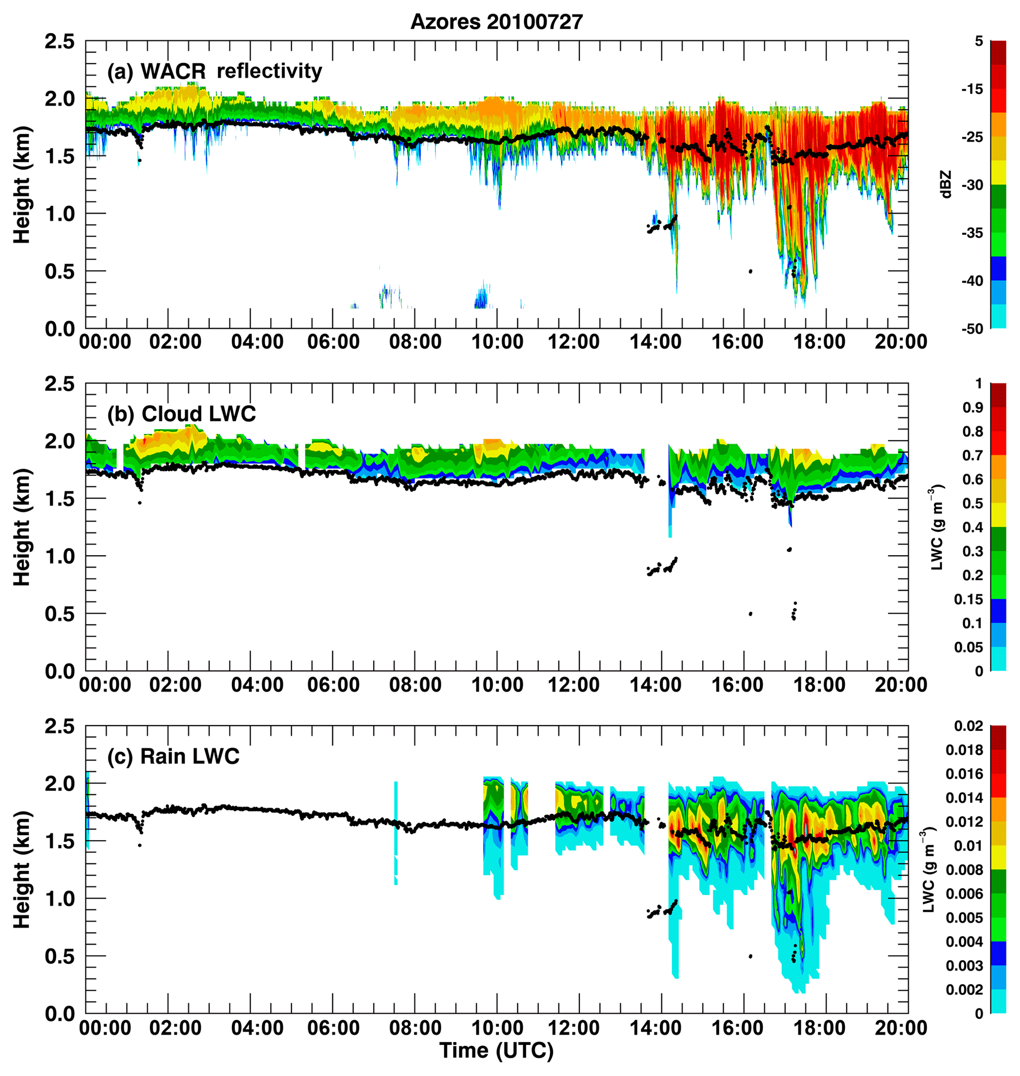
https://www.atmos-chem-phys.net/18/17405/2018/acp-18-17405-2018-f06

Figure A1Joint retrieval of cloud and rain liquid water content (CLWC and RLWC) for the same case as in Fig. 1. (a) WACR reflectivity, (b) CLWC, and (c) RLWC. The black dots represent cloud-base height. Blank gaps are a result of the data from one or more observations being not available or reliable. For example, the gap before 14:00 UTC is due to multiple cloud layers, whereas we only focus on a single layer cloud.

Download

We then compare the CLWC_adiabatic and the one calculated from CLWC_reflectivity at the first range gate above CB. A scale parameter (s) is defined as $s = \frac{{CLWC}_{reflectivity} (1)}{{CLWC}_{adiabatic} (1)}$ , and the entire profile of CLWC_adiabatic is multiplied by s to correct the bias from cloud subadiabaticity. The reflectivity profile from the cloud is then calculated from Eq. (A2.1) using the updated CLWC_adiabatic, and the remaining reflectivity profile from the WACR observation is regarded as the rain contribution. Rain particle size can then be calculated given that N_W and μ are known and rain liquid water content (RLWC) can be estimated.

There are two constraints used in the retrieval. One is that the summation of cloud and rain liquid water path (CLWP and RLWP) must be equal to the LWP from the microwave radiometer observation. Another is that raindrop size (D₀) near cloud top must be equal to or greater than 50 µm, and if D₀ is less than 50 µm, we decrease N_W for the entire rain profile within the cloud and repeat the calculation until the 50 µm criterion is satisfied.

It is difficult to quantitatively estimate the retrieval uncertainties without aircraft in situ measurements. For the proposed retrieval method, 18 % should be used as uncertainty for RLWC from rain properties in Wu et al. (2015) and 30 % for CLWC from cloud properties in Dong et al. (2014a, b). The actual uncertainty depends on the accuracy of the merged sounding data, the sensitivity of WACR near cloud base, and the effect of entrainment on cloud adiabaticity during precipitation. A recent aircraft field campaign, the Aerosol and Cloud Experiments in the Eastern North Atlantic (ACE-ENA), was conducted during 2017–2018 with a total of 39 flights over the Azores, near the ARM ENA site on Graciosa Island. These aircraft in situ measurements will be used to validate the ground-based retrievals and quantitatively estimate their uncertainties in the future.

Figure A1 shows an example of the retrieval results. The merged sounding, ceilometer, microwave radiometer, and WACR are used in the retrieval. Whenever one or more instruments are not reliable, that time step is skipped, and this results in the gaps in the CLWC and RLWC as shown in Fig. A1b and c. When the cloud is classified as non-precipitating, no RLWC will be retrieved. Using air density (ρ_air) profiles calculated from temperature and pressure in merged sounding, mixing ratio (q) can be calculated from LWC using $q (z) = LWC (z) / ρ_{air} (z)$ .

Author contributions

BX, XD, and ZZ initialized this study. PW processed the data and wrote the first draft of the manuscript. All authors contributed to analyzing results. All authors contributed toward revising and improving the manuscript. All authors read and approved the final paper.

Competing interests

The authors declare that they have no conflict of interest.

Acknowledgements

The ground-based measurements were obtained from the Atmospheric Radiation Measurement (ARM) Program sponsored by the US Department of Energy (DOE) Office of Energy Research, Office of Health and Environmental Research, and Environmental Sciences Division. The data can be downloaded from http://www.archive.arm.gov/ (last access: 8 March 2016). This research was supported by the DOE CESM project under grant DE-SC0014641 at the University of Arizona through a subaward from the University of Maryland, Baltimore County, and the NSF project under grant AGS-1700728 at the University of Arizona. The authors thank Yangang Liu at Brookhaven National Laboratory for insightful comments and Ms. Casey E. Oswant at the University of Arizona for proofreading the manuscript. The three anonymous reviewers are acknowledged for constructive comments and suggestions, which helped to improve the manuscript. We appreciate the comments and corrections from the co-editor, Graham Feingold.

Edited by: Graham Feingold
Reviewed by: three anonymous referees

References

Ahlgrimm, M. and Forbes, R.: Improving the Representation of Low Clouds and Drizzle in the ECMWF Model Based on ARM Observations from the Azores, J. Climate, 142, 668–685, https://doi.org/10.1175/MWR-D-13-00153.1, 2014.

Albrecht, B., Fairall, C., Thomson, D., White, A., Snider, J., and Schubert, W.: Surface-based remote-sensing of the observed and the adiabatic liquid water-content of stratocumulus clouds, Geophys. Res. Lett., 17, 89–92, https://doi.org/10.1029/Gl017i001p00089, 1990.

Austin, P., Wang, Y., Kujala, V., and Pincus, R.: Precipitation in Stratocumulus Clouds: Observational and Modeling Results, J. Atmos. Sci., 52, 2329–2352, https://doi.org/10.1175/1520-0469(1995)052<2329:PISCOA>2.0.CO;2, 1995.

Bai, H., Gong, C., Wang, M., Zhang, Z., and L'Ecuyer, T.: Estimating precipitation susceptibility in warm marine clouds using multi-sensor aerosol and cloud products from A-Train satellites, Atmos. Chem. Phys., 18, 1763–1783, https://doi.org/10.5194/acp-18-1763-2018, 2018.

Barker, H. W., Wiellicki, B. A., and Parker, L.: A parameterization for computing grid-averaged solar fluxes for inhomogeneous marine boundary layer clouds. Part II: Validation using satellite data, J. Atmos. Sci., 53, 2304–2316, 1996.

Beheng, K. D.: A parameterization of warm cloud microphysical conversion processes, Atmos. Res., 33, 193–206, 1994.

Bony, S. and Dufresne, J.-L.: Marine boundary layer clouds at the heart of tropical cloud feedback uncertainties in climate models, Geophys. Res. Lett., 32, L20806, https://doi.org/10.1029/2005GL023851, 2005.

Boutle, I. A., Abel, S. J., Hill, P. G., and Morcrette, C. J.: Spatial variability of liquid cloud and rain: Observations and microphysical effects, Q. J. Roy. Meteor. Soc., 140, 583–594, https://doi.org/10.1002/qj.2140, 2014.

Chen, T., Rossow, W. B., and Zhang, Y.: Radiative Effects of Cloud-Type Variations, J. Climate, 13, 264–286, 2000.

Cheng, A. and Xu, K.-M.: A PDF-based microphysics parameterization for simulation of drizzling boundary layer clouds, J. Atmos. Sci., 66, 2317–2334, https://doi.org/10.1175/2009JAS2944.1, 2009.

Comstock, K. K., Yuter, S. E., Wood, R., and Bretherton, C. S.: The Three-Dimensional Structure and Kinematics of Drizzling Stratocumulus, Mon. Weather Rev., 135, 3767–3784, https://doi.org/10.1175/2007MWR1944.1, 2007.

Dong, X., Ackerman, T. P., and Clothiaux, E. E.: Parameterizations of Microphysical and Radiative Properties of Boundary Layer Stratus from Ground-based measurements, J. Geophys. Res., 102, 31681–31393, 1998.

Dong, X., Minnis, P., Ackerman, T. P., Clothiaux, E. E., Mace, G. G., Long, C. N., and Liljegren, J. C.: A 25-month database of stratus cloud properties generated from ground-based measurements at the ARM SGP site, J. Geophys. Res., 105, 4529–4538, 2000.

Dong, X., Xi, B., Kennedy, A., Minnis, P., and Wood, R.: A 19-month Marine Aerosol-Cloud_Radiation Properties derived from DOE ARM AMF deployment at the Azores: Part I: Cloud Fraction and Single-layered MBL cloud Properties, J. Climate, 27, 3665–3682, https://doi.org/10.1175/JCLI-D-13-00553.1, 2014a.

Dong, X., Xi, B., and Wu, P.: Investigation of Diurnal Variation of MBL Cloud Microphysical Properties at the Azores, J. Climate, 27, 8827–8835, 2014b.

Fielding, M. D., Chiu, J. C., Hogan, R. J., Feingold, G., Eloranta, E., O'Connor, E. J., and Cadeddu, M. P.: Joint retrievals of cloud and drizzle in marine boundary layer clouds using ground-based radar, lidar and zenith radiances, Atmos. Meas. Tech., 8, 2663–2683, https://doi.org/10.5194/amt-8-2663-2015, 2015.

Frisch, A., Fairall, C., and Snider, J.: Measurement of stratus cloud and drizzle parameters in ASTEX with a Ka-band Doppler radar and a microwave radiometer, J. Atmos. Sci., 52, 2788–2799, 1995.

Geoffroy, O., Brenguier, J.-L., and Burnet, F.: Parametric representation of the cloud droplet spectra for LES warm bulk microphysical schemes, Atmos. Chem. Phys., 10, 4835–4848, https://doi.org/10.5194/acp-10-4835-2010, 2010.

Hahn, C. and Warren, S.: A gridded climatology of clouds over land (1971–96) and ocean (1954–97) from surface observations worldwide, Numeric Data Package NDP-026E ORNL/CDIAC-153, CDIAC, Department of Energy, Oak Ridge, Tennessee, 2007.

Hartmann, D. L., Ockert-Bell, M. E., and Michelsen, M. L.: The Effect of Cloud Type on Earth's Energy Balance: Global Analysis, J. Climate, 5, 1281–1304, https://doi.org/10.1175/1520?0442(1992)005<1281:TEOCTO>2.0.CO;2, 1992.

Hartmann, D. L. and Short, D. A.: On the use of earth radiation budget statistics for studies of clouds and climate, J. Atmos. Sci., 37, 1233–1250, https://doi.org/10.1175/1520-0469(1980)037<1233:OTUOER>2.0.CO;2, 1980.

Hill, P. G., Morcrette, C. J., and Boutle, I. A.: A regime-dependent parametrization of subgrid-scale cloud water content variability, Q. J. Roy. Meteorol. Soc., 141, 1975–1986, 2015.

Houghton, J. T., Ding, Y., Griggs, D. J., Noguer, M., van der Linden, P. J., Dai, X., Maskell, K., and Johnson, C. A.: Climate Change: The Scientific Basis, Cambridge University Press, 881 pp., 2001.

Jess, S.: Impact of subgrid variability on large-scale precipitation formation in the climate model ECHAM5, PhD thesis, Dep. of Environ. Syst. Sci., ETH Zurich, Zurich, Switzerland, 2010.

Jiang, J., Su, H., Zhai, C., Perun, V. S., Del Genio, A., Nazarenko, L. S., Donner, L. J., Horowitz, Seman, L., Cole, C., J., Gettelman, A., Ringer, M. A., Rotstayn, L., Jeffrey, S., Wu, T., Brient, F., Dufresne, J-L., Kawai, H., Koshiro, T., Watanabe, M., LÉcuyer, T. S., Volodin, E. M., Iversen, Drange, T., H., Mesquita, M. D. S., Read, W. G., Waters, J. W., Tian, B., Teixeira, J., and Stephens, G. L.: Evaluation of cloud and water vapor simulations in CMIP5 climate models using NASA “A-train” satellite observations, J. Geophys. Res., 117, D14105, https://doi.org/10.1029/2011JD017237, 2012.

Kessler, E.: On the distribution and continuity of water substance in atmospheric circulations, Met. Monograph 10, No. 32, American Meteorological Society, Boston, USA, 84 pp., 1969.

Khairoutdinov, M. and Kogan, Y.: A New Cloud Physics Parameterization in a Large-Eddy Simulation Model of Marine Stratocumulus, Mon. Weather Rev., 128, 229–243, 2000.

Kollias, P., Szyrmer, W., Rémillard, J., and Luke, E.: Cloud radar Doppler spectra in drizzling stratiform clouds:2. Observations and microphysical modeling of drizzle evolution, J. Geophys. Res., 116, D13203, https://doi.org/10.1029/2010JD015238, 2011.

Kubar, T. L., Hartmann, D. L., and Wood, R.: Understanding the importance of microphysics and macrophysics in marine low clouds, Part I: satellite observations, J. Atmos. Sci., 66, 2953–2972, https://doi.org/10.1175/2009JAS3071.1, 2009.

Larson, V. E. and Griffin, B. M.: Analytic upscaling of a local microphysics scheme. Part I: Derivation, Q. J. Roy. Meteor. Soc., 139, 46–57, 2013.

Larson, V. E., Nielsen, B. J., Fan, J., and Ovchinnikov, M.: Parameterizing correlations between hydrometeor species in mixed-phase Arctic clouds, J. Geophys. Res., 116, D00T02, https://doi.org/10.1029/2010JD015570, 2011.

Lebsock, M. D., Morrison, H., and Gettelman, A.: Microphysical implications of cloud-precipitation covariance derived from satellite remote sensing, J. Geophys. Res.-Atmos., 118, 6521–6533, https://doi.org/10.1002/jgrd.50347, 2013.

Lee, H. and Baik, J.-J.: A physically based autoconversion parameterization, J. Atmos. Sci., 74, 1599–1616, 2017.

Leon, D. C., Wang, Z., and Liu, D.: Climatology of drizzle in marine boundary layer clouds based on 1 year of data from CloudSat and Cloud-Aerosol Lidar and Infrared Pathfinder Satellite Observations (CALIPSO), J. Geophys. Res., 113, D00A14, https://doi.org/10.1029/2008JD009835, 2008.

Liljegren, J. C., Clothiaux, E. E., Mace, G. G., Kato, S., and Dong, X.: A new retrieval for cloud liquid water path using a ground-based microwave radiometer and measurements of cloud temperature, J. Geophys. Res., 106, 14485–14500, 2001.

Liu, Y. and Daum, P. H.: Parameterization of the autoconversion process, Part I: Analytical formulation of the Kessler-type parameterizations, J. Atmos. Sci., 61, 1539–1548, 2004.

Liu, Y., Daum, P. H., and McGraw, R.: Parameterization of the autoconversion process. Part II: Generalization of Sundqvist-type parameterizations, J. Atmos. Sci., 63, 1103–1109, 2006a.

Liu, Y., Daum, P. H., McGraw, R., and Miller, M.: Generalized threshold function accounting for effect of relative dispersion on threshold behavior of autoconversion process, Geophys. Res. Lett., 33, L11804, https://doi.org/10.1029/2005GL025500, 2006b.

Michibata, T. and Takemura, T.: Evaluation of autoconversion schemes in a single model framework with satellite observations, J. Geophys. Res.-Atmos., 120, 9570–9590, https://doi.org/10.1002/2015JD023818, 2015.

Miles, N. L., Verlinde, J., and Clothiaux, E. E.: Cloud-droplet size distributions in low-level stratiform clouds. J. Atmos. Sci., 57, 295–311, https://doi.org/10.1175/1520-0469(2000)057, 2000.

Morrison, H. and Gettelman, A.: A new two-moment bulk stratiform cloud microphysics scheme in the Community Atmosphere Model, version 3 (CAM3). Part I: Description and numerical tests, J. Climate, 21, 3642–3659, 2008.

Nam, C. and Quaas, J.: Evaluation of clouds and precipitation in the ECHAM5 general circulation model using CALIPSO and CloudSat satellite data, J. Climate, 25, 4975–4992, https://doi.org/10.1175/JCLI-D-11-00347.1, 2012.

O'Connor, E. J., Hogan, R. J., and Illingworth, A. J.: Retrieving stratocumulus drizzle parameters using Doppler radar and lidar, J. Appl. Meteorol., 44, 14–27, 2005.

Pincus, R. and Klein, S. A.: Unresolved spatial variability and microphysical process rates in large-scale models, J. Geophys. Res., 105D, 27059–27065, 2000.

Pincus, R., McFarlane, S. A., and Klein, S. A.: Albedo bias and the horizontal variability of clouds in subtropical marine boundary layers: Observations from ships and satellites, J. Geophys. Res., 104, 6183–6191, https://doi.org/10.1029/1998JD200125, 1999.

Platnick, S. and Twomey, S.: Determining the Susceptibility of Cloud Albedo to Changes in Droplet Concentration with the Advanced Very High Resolution Radiometer, J. Appl. Meteorol., 33, 334–347, 1994.

Randall, D. A., Coakley, J. A., Fairall, C. W., Knopfli, R. A., and Lenschow, D. H.: Outlook for research on marine subtropical stratocumulus clouds, B. Am. Meteorol. Soc., 65, 1290–1301, 1984.

Rémillard, J., Kollias, P., Luke, E., and Wood, R.: Marine Boundary Layer Cloud Observations in the Azores, J. Climate, 25, 7381–7398, doi:https://doi.org/10.1175/JCLI-D-11-00610.1, 2012.

Rémillard, J., Kollias, P., and Szyrmer, W.: Radar-radiometer re- trievals of cloud number concentration and dispersion parameter in nondrizzling marine stratocumulus, Atmos. Meas. Tech., 6, 1817–1828, https://doi.org/10.5194/amt-6-1817-2013, 2013.

Sauvageot, H. and Omar, J.: Radar reflectivity of cumulus clouds, J. Atmos. Ocean. Technol., 4, 264–272, 1987.

Slingo, A.: Sensitivity of the Earth's radiation budget to changes in low clouds, Nature, 343, 49–51, https://doi.org/10.1038/343049a0, 1990.

Song, H., Zhang, Z., Ma, P.-L., Ghan, S. J., and Wang, M.: An Evaluation of Marine Boundary Layer Cloud Property Simulations in the Community Atmosphere Model Using Satellite Observations: Conventional Subgrid Parameterization versus CLUBB, J. Climate, 31, 2299–2320, https://doi.org/10.1175/JCLI-D-17-0277.1, 2018.

Stanfield, R., Dong, X., Xi, B., Gel Genio, A., Minnis, P., and Jiang, J.: Assessment of NASA GISS CMIP5 and post CMIP5 Simulated Clouds and TOA Radiation Budgets Using Satellite Observations: Part I: Cloud Fraction and Properties, J. Climate, 27, 4189–4208, 2014.

Stephens, G. L., L'Ecuyer, T., Forbes, R., Gettlemen, A., Golaz, J.-C., Bodas-Salcedo, A., Suzuki, K., Gabriel, P., and Haynes, J.: Dreary state of precipitation in global models, J. Geophys. Res., 115, D24211, https://doi.org/10.1029/2010JD014532, 2010.

Tripoli, G. J. and Cotton, W. R.: A numerical investigation of several factors contributing to the observed variable intensity of deep convection over South Florida, J. Appl. Meteorol., 19, 1037–1063, 1980.

Troyan, D.: Merged Sounding Value-Added Product, Tech. Rep., DOE/SC-ARM/TR-087, 2012.

Walters, D., Baran, A., Boutle, I., Brooks, M., Earnshaw, P., Edwards, J., Furtado, K., Hill, P., Lock, A., Manners, J., Morcrette, C., Mulcahy, J., Sanchez, C., Smith, C., Stratton, R., Tennant, W., Tomassini, L., Van Weverberg, K., Vosper, S., Willett, M., Browse, J., Bushell, A., Dalvi, M., Essery, R., Gedney, N., Hardiman, S., Johnson, B., Johnson, C., Jones, A., Mann, G., Milton, S., Rumbold, H., Sellar, A., Ujiie, M., Whitall, M., Williams, K., and Zerroukat, M.: The Met Office Unified Model Global Atmosphere 7.0/7.1 and JULES Global Land 7.0 configurations, Geosci. Model Dev. Discuss., https://doi.org/10.5194/gmd-2017-291, in review, 2017.

Wang, J. and Geerts, B.: Identifying drizzle within marine stratus with W-band radar reflectivity, Atmos. Res., 69, 1–27, 2003.

Wang, M., Ghan, S., Liu, X., L'Ecuyer, T. S., Zhang, K., Morrison, H., Ovchinnikov, M., Easter, R., Marchand, R., Chand, D., Qian, Y., and Penner, J. E.: Constraining cloud lifetime effects of aerosols using A-Train satellite observations, Geophys. Res. Lett., 39, L15709, https://doi.org/10.1029/2012GL052204, 2012.

Warren, S. G., Hahn, C. J., London, J., Chervin, R. M., and Jenne, R.: Global distribution of total cloud cover and cloud type amount over land, Tech. Rep. Tech. Note TN-317 STR, NCAR, 1986.

Warren, S. G., Hahn, C. J., London, J., Chervin, R. M., and Jenne, R.: Global distribution of total cloud cover and cloud type amount over land, Tech. Rep. Tech. Note TN-317 STR, NCAR, 1988.

Weber, T. and Quaas, J.: Incorporating the subgrid-scale variability of clouds in the autoconversion parameterization using a PDF-scheme, J. Adv. Model. Earth Syst., 4, M11003, https://doi.org/10.1029/2012MS000156, 2012.

Wielicki, B. A., Cess, R. D., King, M. D., Randall, D. A., and Harrison, E. F.: Mission to planet Earth: Role of clouds and radiation in climate, B. Am. Meteorol. Soc., 76, 2125–2153, https://doi.org/10.1175/1520-0477(1995)076<2125:MTPERO>2.0.CO;2, 1995.

Witte, M. K., Yuan, T., Chuang, P. Y., Platnick, S., Meyer, K. G., Wind, G., and Jonsson, H. H.: MODIS retrievals of cloud effective radius in marine stratocumulus exhibit no significant bias, Geophys. Res. Lett., 45, 10656–10664, https://doi.org/10.1029/2018GL079325, 2018.

Wood, R.: Drizzle in stratiform boundary layer clouds. Part I: Vertical and horizontal structure, J. Atmos. Sci., 62, 3011–3033, 2005a.

Wood, R.: Drizzle in stratiform boundary layer clouds. Part II: Microphysical aspects, J. Atmos. Sci., 62, 3034–3050, 2005b.

Wood, R.: Stratocumulus Clouds, Mon. Weather Rev., 140, 2373–2423, https://doi.org/10.1175/MWR-D-11-00121.1, 2012.

Wood, R. and Hartmann, D.: Spatial variability of liquid water path in marine low cloud: The importance of mesoscale cellular convection, J. Climate, 19, 1748–1764, 2006.

Wood, R., Field, P. R., and Cotton, W. R.: Autoconversion rate bias in stratiform boundary layer cloud parameterization, Atmos. Res., 65, 109–128, 2002.

Wood, R., Wyant, M., Bretherton, C. S., Rémillard, J., Kollias, P., Fletcher, J., Stemmler, J., deSzoeke, S., Yuter, S., Miller, M., Mechem, D., Tselioudis, G., Chiu, C., Mann, J., O'Connor, E., Hogan, R., Dong, X., Miller, M., Ghate, V., Jefferson, A., Min, Q., Minnis, P., Palinkonda, R., Albrecht, B., Luke, E., Hannay, C., and Lin, Y.: Clouds, Aerosol, and Precipitation in the Marine Boundary Layer: An ARM Mobile Facility Deployment, B. Am. Meteorol. Soc., https://doi.org/10.1175/BAMS-D-13-00180.1, 2015.

Wu, P., Dong, X., and Xi, B.: Marine boundary layer drizzle properties and their impact on cloud property retrieval, Atmos. Meas. Tech., 8, 3555–3562, https://doi.org/10.5194/amt-8-3555-2015, 2015.

Wu, P., Dong, X., Xi, B., Liu, Y., Thieman, M., and Minnis, P.: Effects of environment forcing on marine boundary layer cloud-drizzle processes, J. Geophys. Res.-Atmos., 122, 4463–4478, https://doi.org/10.1002/2016JD026326, 2017.

Xie, X. and Zhang, M.: Scale-aware parameterization of liquid cloud inhomogeneity and its impact on simulated climate in CESM, J. Geophys. Res.-Atmos., 120, 8359–8371, https://doi.org/10.1002/2015JD023565, 2015.

Yoo, H. and Li, Z.: Evaluation of cloud properties in the NOAA/NCEP Global Forecast System using multiple satellite products, Clim. Dynam., 39, 2769–2787, https://doi.org/10.1007/s00382-012-1430-0, 2012.

Yoo, H., Li, Z., Hou, Y.-T., Lord, S., Weng, F., and Barker, H. W.: Diagnosis and testing of low-level cloud parameterizations for the NCEP/GFS using satellite and ground-based measurements, Clim. Dynam., 41, 1595–1613, https://doi.org/10.1007/s00382-013-1884-8, 2013.

Zhang, J., Lohmann, U., and Lin, B.: A new statistically based autoconversion rate parameterization for use in large-scale models, J. Geophys. Res., 107, 4750, https://doi.org/10.1029/2001JD001484, 2002.

Zhang, Z., Song, H., Ma, P.-L., Larson, V., Wang, M., Dong, X., and Wang, J.: Subgrid variations of cloud water and droplet number concentration over tropical oceans: satellite observations and implications for warm rain simulation in climate models Atmos. Chem. Phys., submitted, 2018.

Articles

Short summary

Prescribed autoconversion and accretion enhancement factors in GCM warm-rain parameterizations contribute partially to the too-frequent and too-light problem in precipitation simulation. The two factors should be regime- and resolution-dependent. A decreased autoconversion enhancement factor and increased accretion enhancement factor in the Morrison and Gettleman (2008) scheme can improve the simulated precipitation frequency and intensity. The two factors for other schemes are also suggested.