the Creative Commons Attribution 4.0 License.
the Creative Commons Attribution 4.0 License.
 | 07 Dec 2018
Computation and analysis of atmospheric carbon dioxide annual mean growth rates from satellite observations during 2003–2016
Michael Buchwitz
Maximilian Reuter
Oliver Schneising
Stefan Noël
Bettina Gier
Heinrich Bovensmann
John P. Burrows
Hartmut Boesch
Jasdeep Anand
Robert J. Parker
Peter Somkuti
Rob G. Detmers
Otto P. Hasekamp
Ilse Aben
André Butz
Akihiko Kuze
Hiroshi Suto
Yukio Yoshida
David Crisp
Christopher O'Dell
The growth rate of atmospheric carbon dioxide (CO2) reflects the net effect of emissions and uptake resulting from anthropogenic and natural carbon sources and sinks. Annual mean CO2 growth rates have been determined from satellite retrievals of column-averaged dry-air mole fractions of CO2, i.e. XCO2, for the years 2003 to 2016. The XCO2 growth rates agree with National Oceanic and Atmospheric Administration (NOAA) growth rates from CO2 surface observations within the uncertainty of the satellite-derived growth rates (mean difference ± standard deviation: 0.0±0.3 ppm year−1; R: 0.82). This new and independent data set confirms record-large growth rates of around 3 ppm year−1 in 2015 and 2016, which are attributed to the 2015–2016 El Niño. Based on a comparison of the satellite-derived growth rates with human CO2 emissions from fossil fuel combustion and with El Niño Southern Oscillation (ENSO) indices, we estimate by how much the impact of ENSO dominates the impact of fossil-fuel-burning-related emissions in explaining the variance of the atmospheric CO2 growth rate. Our analysis shows that the ENSO impact on CO2 growth rate variations dominates that of human emissions throughout the period 2003–2016 but in particular during the period 2010–2016 due to strong La Niña and El Niño events. Using the derived growth rates and their uncertainties, we estimate the probability that the impact of ENSO on the variability is larger than the impact of human emissions to be 63 % for the time period 2003–2016. If the time period is restricted to 2010–2016, this probability increases to 94 %.
- Article
(3156 KB) - Full-text XML
- BibTeX
- EndNote


Atmospheric carbon dioxide (CO2) is an important greenhouse gas that causes global warming (IPCC, 2013). Sources that emit CO2 into the atmosphere include anthropogenic and natural sources at the surface, and the oxidation of carbon monoxide and hydrocarbons in the atmosphere. The sinks that remove CO2 primarily at the surface include biological (photosynthesis) and physical (solubility) processes. Anthropogenic emissions of CO2, primarily from fossil fuel combustion, have increased the atmospheric CO2 mixing ratios at the surface by more than 40 % since pre-industrial times, from less than 280 parts per million (ppm) to 402.8±0.1 ppm in 2016 (Dlugokencky and Tans, 2017a). A global increase of atmospheric CO2 by 1 ppm in a 1-year time period corresponds to an annual increase of 2.12 GtC year−1 (Ballantyne et al., 2012). However, this increase in mass does not directly correspond to the emissions. The reason is that only a fraction of the emitted CO2 remains in the atmosphere, as CO2 is partitioned between the atmosphere and ocean and land carbon sinks. On average, somewhat less than half of the emitted CO2 remains in the atmosphere but this “airborne fraction” varies substantially from year to year (Le Quéré et al., 2016, 2018). Variations of the airborne fraction are not well understood, primarily because of an inadequate understanding of the terrestrial carbon sink, which introduces large uncertainties for climate prediction (e.g. IPCC, 2013; Peylin et al., 2013; Wieder et al., 2015; Huntzinger et al., 2017). Identification of the origin of changes in the growth rate requires additional information for the attribution to particular sources or sinks (Peters et al., 2017). Atmospheric CO2 growth rates inferred from in situ CO2 surface measurements are regularly determined and published, for example by the National Oceanic and Atmospheric Administration (NOAA) (see https://www.esrl.noaa.gov/gmd/ccgg/trends/gr.html, last access: 24 November 2017). In this study, we present and interpret atmospheric growth rates determined from the remote sensing of CO2 vertical columns from space, which are described in the following section.
Satellites provide retrievals of CO2 vertical columns in terms of the CO2 column-averaged dry-air mole fraction, denoted by XCO2. Although it is a relatively new field, satellite-based XCO2 data products have already been used to improve our knowledge of natural (e.g. Basu et al., 2013; Maksyutov et al., 2013; Chevallier et al., 2014; Reuter et al., 2014a; Schneising et al., 2014; Houweling et al., 2015; Parker et al., 2016; Heymann et al., 2017; Kaminski et al., 2017; Liu et al., 2017) and anthropogenic (e.g. Schneising et al., 2013; Reuter et al., 2014b; Kort et al., 2012; Hakkarainen et al., 2016; Nassar et al., 2017) CO2 sources and sinks, but only a few studies explicitly present and discuss CO2 growth rates. Buchwitz et al. (2007), analysed the first 3 years (2003–2005) of XCO2 retrievals from SCIAMACHY-ENVISAT (Burrows et al., 1995; Bovensmann et al., 1999) generated using the WFM-DOAS retrieval algorithm (Buchwitz et al., 2006). They computed year-to-year CO2 variations and compared the XCO2 increase with the XCO2 increase computed from the output of NOAA's CO2 assimilating system CarbonTracker (Peters et al., 2007) and found agreement within 1 ppm year−1. Schneising et al., 2014 computed growth rates from the 2003–2011 SCIAMACHY XCO2 record. They compared the derived annual growth rates with surface temperature and found that years having higher temperatures during the vegetation growing season are associated with larger growth rates in atmospheric CO2 at northern midlatitudes. Growth rates from GOSAT (Kuze et al., 2016) are published by the National Institute for Environmental Studies (NIES), Tsukuba, Japan (NIES, 2017).
Table 1Satellite XCO2 data products. Individual satellite sensor XCO2 algorithms and corresponding level 2 data products used for generating the EMMAv3 level 2 (i.e. individual soundings) data product, which has been gridded to obtain the O4Mv3 level 3 data product used in this study. GHG-CCI refers to the GHG-CCI project of ESA's Climate Change Initiative (http://www.esa-ghg-cci.org/, last access: 10 October 2017) and C3S is the Copernicus Climate Change Service (https://climate.copernicus.eu/, last access: 11 January 2018).
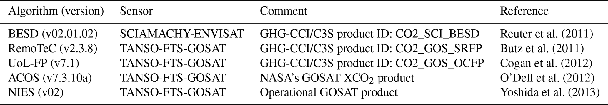
In this study, we analyse a new satellite XCO2 data set covering 14 years (2003–2016) generated from SCIAMACHY-ENVISAT and TANSO-FTS-GOSAT. We use the XCO2 data product Obs4MIPs (Observations for Model Intercomparisons Project) version 3 (O4Mv3), which is a gridded (level 3) monthly data product at 5∘ latitude by 5∘ longitude spatial resolution in Obs4MIPs format (Buchwitz et al., 2017a). Obs4MIPs (https://www.earthsystemcog.org/projects/obs4mips/, last access: 10 October 2018) is an activity to make observational products more accessible for climate model intercomparisons (e.g. Lauer et al., 2017). The O4Mv3 XCO2 data product was generated by gridding (averaging) the XCO2 level 2 (i.e. individual soundings) product generated with the ensemble median algorithm (EMMA, Reuter et al., 2013). EMMA uses as input an ensemble of XCO2 level 2 data products (Reuter et al., 2013; Buchwitz et al., 2015, 2017a, b) from SCIAMACHY-ENVISAT and TANSO-FTS-GOSAT. To generate the O4Mv3 product, the EMMA version 3.0 (EMMAv3, Reuter et al., 2017c) product was used. The list of satellite products used for the generation of the EMMAv3 level 2 product – and therefore also for the O4Mv3 level 3 data product used in this study – is provided in Table 1. The quality of this product relative to Total Carbon Column Observing Network (TCCON) ground-based observations (Wunch et al., 2011, 2015) can be summarized as follows (Buchwitz et al., 2017c): +0.23 ppm overall (global) bias, relative accuracy 0.3 ppm (1σ), and very good stability in terms of a linear bias trend ( ppm year−1).
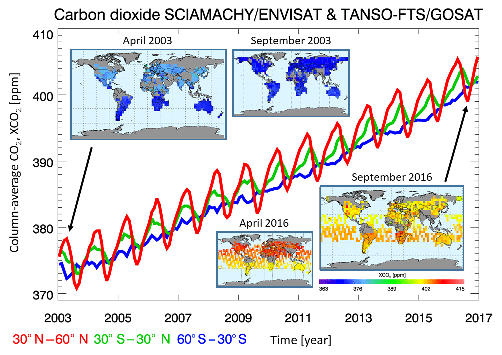
Figure 1Time series and global maps of satellite-derived column-averaged dry-air mole fractions of carbon dioxide, i.e. XCO2. Data product Obs4MIPs version 3 is shown (O4Mv3) based on an ensemble of SCIAMACHY-ENVISAT (until April 2012) and TANSO-FTS-GOSAT (since mid-2009) individual sensor and individual sounding (level 2) data products. The three time series correspond to three latitude bands: 30–60∘N (red), 30∘ S–30∘N (green) and 60–30∘S (blue). The maps in the top left show monthly XCO2 for April and September 2003 (SCIAMACHY, land only) and the maps on the bottom right show monthly XCO2 for April and September 2016 (TANSO-FTS, land and ocean glint).
Figure 1 presents an overview of the O4Mv3 product in terms of time series and global XCO2 maps. The maps show the typical coverage of XCO2 from SCIAMACHY (until April 2012) and GOSAT (since mid-2009). As can be seen, the time series for the three latitude bands shown in Fig. 1 have very similar slopes. They mainly differ in the amplitude of the seasonal cycle, which reflects the latitudinal dependence of uptake and release of atmospheric CO2 by the terrestrial biosphere (Schneising et al., 2014). These time series have been used to compute annual mean CO2 growth rates as will be explained in the following section.
The National Oceanic and Atmospheric Administration (NOAA) defines the annual mean CO2 growth rate for a given year as the CO2 concentration difference at the end of that year minus the CO2 concentration at the beginning of that year (Thoning et al., 1989; see also additional explanations given on the NOAA/ESRL website; https://www.esrl.noaa.gov/gmd/ccgg/about/global_means.html, last access: 10 October 2017). As described below, our method involves the following three steps: (i) computation of an XCO2 time series (at monthly resolution and sampling) by averaging the XCO2 in the region of interest (e.g. a latitude band; see Appendix A, Fig. A1); (ii) computation of monthly sampled XCO2 annual growth rates by computing the difference of the XCO2 value of month i minus the XCO2 value of month i-12 and computation of the corresponding uncertainty estimate; (iii) computation of annual mean growth rates and their corresponding uncertainties from the monthly sampled annual growth rates.
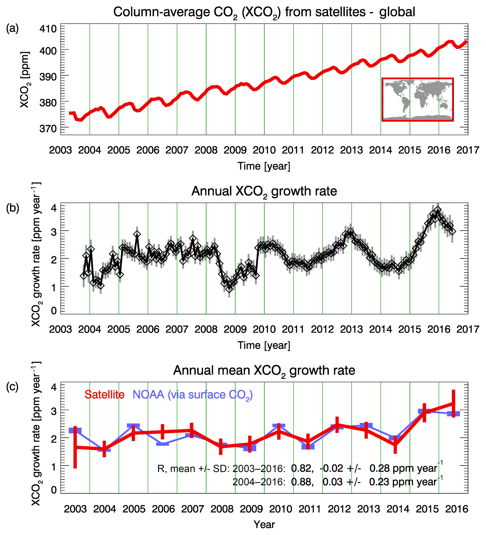
Figure 2Atmospheric CO2 and corresponding growth rates. (a) Monthly mean XCO2 (red line) as obtained from averaging XCO2 data product O4Mv3 globally for each month. (b) Monthly sampled annual CO2 growth rates computed from the red curve shown in (a) including 1σ uncertainty (grey vertical bars). (c) Annual mean growth rates computed from averaging the values shown in (b) including 1σ error estimates (vertical bars) (the numerical values are listed in Table A1 of Appendix A). The NOAA annual mean global growth rate is also shown in (c) for comparison (in blue). Also listed in (c) is the linear correlation coefficient (R), the mean difference and the standard deviation of the difference between the satellite and the NOAA growth rates for 2003–2016 and for 2004–2016.
In the following, this method is described in detail using Fig. 2 for illustration. In Fig. 2a monthly satellite XCO2 (O4Mv3) is plotted, obtained by globally averaging all the individual () XCO2 values. To compute the spatially averaged XCO2 time series (shown in Fig. 2a), we first longitudinally average the XCO2 followed by the computation of the area-weighted latitudinal average of XCO2 by using the cosine of latitude as weight. We consider surface area because surface fluxes are linked to mass of CO2 (or number of CO2 molecules) rather than molecular mixing ratios or mole fractions. As can be seen, the computed time series does not start at the beginning of 2003 but in April 2003. As explained in Buchwitz et al. (2017d) (see discussion of their Fig. 6.1.1.1), the underlying SCIAMACHY BESD v02.01.02 XCO2 data product (see Table 1) apparently suffers from an approximately 1 ppm high bias in the first few months of 2003. The exact magnitude of this bias has not been quantified due to a lack of TCCON validation data in this early time period. As this bias in early 2003 is critical for the year 2003 growth rate, we have omitted the first 3 months of 2003 for the computation of the growth rates shown in this publication.
Figure 2b shows monthly sampled annual growth rates computed from the monthly XCO2 values shown in Fig. 2a. Each value is the difference between two monthly XCO2 values corresponding to the same month (e.g. January) but different years (e.g. 2004 and 2005). For example, the first data point (first diamond symbol) shown in Fig. 2b is the difference of the April 2004 XCO2 value minus the April 2003 XCO2 value. The second data point corresponds to May 2004 minus May 2003, etc. The time difference between the monthly XCO2 pairs is always 1 year and the time assigned to each XCO2 difference is the time in the middle of that year. Therefore, the time series shown in Fig. 2b starts 6 months later and ends 6 months earlier compared to the time series shown in Fig. 2a. Each XCO2 difference shown in Fig. 2b therefore corresponds to an estimate of the XCO2 annual growth rate and the position on the time axis corresponds to the middle of the corresponding 1-year time period.
A 1σ uncertainty estimate has been computed for each of the monthly sampled annual growth rates shown in Fig. 2b (see grey vertical bars). They have been computed such that they reflect the following aspects: (i) the standard error of the O4Mv3 XCO2 values as given in the O4Mv3 data product file for each of the grid cells, (ii) the spatial variability of the XCO2 within the selected region, (iii) the temporal variability of the annual growth rates in the 1-year time interval, which corresponds to the annual growth rate, and (iv) the number of months (N) with data located in that 1-year time interval. The uncertainties have been computed as the mean value of three terms divided by the square root of N. The first term is the mean value of the standard error, the second term is the standard deviation of the XCO2 values in the selected region and the third term is the standard deviation of the monthly sampled annual growth rates in the corresponding 1-year time interval. We aimed to provide realistic error estimates but we acknowledge that our uncertainty estimates are not based on full error propagation, which would be difficult, especially due to unknown or not well enough known systematic errors and error correlations. The reported uncertainty estimates should therefore be interpreted as error indications rather than fully rigorous error estimates.
Figure 2c shows the final result, i.e. the annual mean XCO2 growth rates and their estimated (1σ) uncertainties. The annual mean growth rates have been computed by averaging all the monthly sampled annual growth rates (shown in Fig. 2b), which are located in the year of interest (e.g. 2003). For most years, 12 annual growth rate values are available for averaging but there are some exceptions. For example, for the year 2003 only three values are present, as can be seen from Fig. 2b, and for the years 2014 and 2015 there are only 11 values, as no data are available for January 2015 due to issues with the GOSAT satellite. The uncertainty of the annual mean growth rate has been computed by averaging the uncertainties assigned to each of the monthly sampled annual growth rates (shown as grey vertical bars in Fig. 2b) scaled with a factor, which depends on the number of months (N) available for averaging. This factor is the square root of 12/N. It ensures that the larger the uncertainty, the fewer data points there are available for averaging. Overall, our uncertainty estimate is quite conservative, as we do not assume that errors improve upon averaging. As a result of this procedure, the error bar of the year 2003 growth rate is quite large (0.76 ppm year−1; see Table A1 in Appendix A, where all numerical values are listed). This is because the monthly sampled annual growth rate varies significantly in 2003 (see Fig. 2b) and because only N=3 data points are available for averaging in 2003. In contrast, the year 2005 growth rate uncertainty is much smaller (0.28 ppm year−1), because the growth rates vary less during 2005 and because N=12 data points are available for averaging.
In Fig. 2c the NOAA global growth rates (Dlugokencky and Tans, 2017b) are also shown. As can be seen, the satellite-derived growth rates agree well with the NOAA growth rates obtained from CO2 surface observations. For the time period 2003–2016 the linear correlation coefficient R is 0.82 and the difference is ppm year−1 (mean difference ± standard deviation). Perfect agreement is not to be expected as these two growth rate time series have been obtained from CO2 observations which represent very different vertical samplings of the atmosphere (surface (NOAA) versus entire vertical column (satellite); see Fig. A3b in Appendix A for a comparison of XCO2 and surface CO2 growth rates obtained using a global reanalysis CO2 data product). Perfect agreement is also not to be expected because we use different time periods for the computation of the annual growth rates compared to NOAA (see Fig. A3c in Appendix A for a comparison of two different methods to compute annual XCO2 growth rates).
As can also be seen from Fig. 2c, the largest growth rates are approximately 3 ppm year−1 during 2015 and 2016. These record-large growth rates (Peters et al., 2017) are attributed to the consequences of the strong 2015–2016 El Niño event, which produced large CO2 emissions from fires and enhanced net biospheric respiration in the tropics relative to normal conditions (Heymann et al., 2017; Liu et al., 2017). Many of these fires are initiated by humans, for example, to clear tropical forests. In this study, human emissions of CO2 are defined as emissions from fossil fuel combustion and industry (Le Quéré et al., 2016, 2018) but do not include, for example, CO2 emissions originating from slash and burn agriculture.
It is well known that changes in the growth rate of atmospheric CO2 have anthropogenic and natural causes (e.g. Jones et al., 2001; Betts et al., 2016; Kim et al., 2016; Liu et al., 2017; Chylek et al., 2018). In this section we are aiming at answering the following question: “Assuming that the variability of the CO2 growth rate is dominated by ENSO and by human emissions, which of the two considered causes dominates the growth rate variability given the satellite-derived growth rates and their uncertainty?”. To answer this question we are using a simple linear statistical model and time series of human emissions and two ENSO indices, assuming that these indices are appropriate proxies for ENSO-related effects in the context of providing a reliable answer.
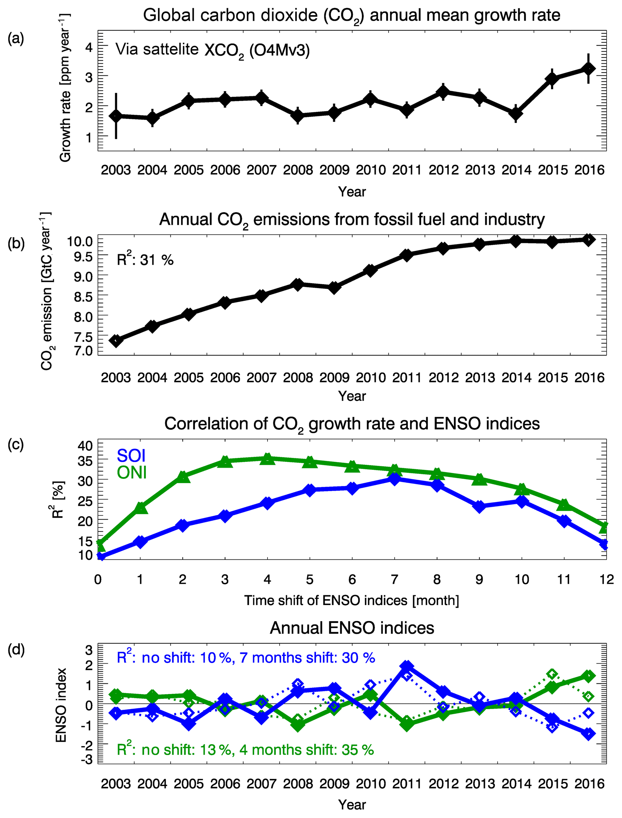
Figure 3Carbon dioxide global annual mean growth rates compared with human emissions and ENSO indices. (a) Satellite-derived global annual mean growth rates (with 1σ uncertainty range shown as vertical lines). (b) CO2 emissions from fossil fuel and industry (the correlation with the growth rate is R2=31 %). (c) Correlation in terms of R2 of growth rate and annual SOI (blue curve) and ONI (green curve) as a function of time shift in months. (d) Annual SOI for no shift (blue dotted line, R2=10 %) and for a shift of 7 months (blue solid line, R2=30 %) and annual ONI for no shift (green dotted line, R2=13 %) and for a shift of 4 months (green solid line, R2=35 %).
Figure 3 shows a comparison of the CO2 annual mean growth rates (Fig. 3a) with annual global CO2 emissions from fossil fuel combustion and industry (Fig. 3b) (Le Quéré et al., 2018; GCP, 2017) (correlation of growth rate and human emissions: R2=31 %). As can be seen, the growth rates vary significantly in recent years despite nearly constant human emissions. Figure 3d shows two ENSO indices: the Southern Oscillation Index (SOI, blue lines) (Ropelewski and Jones, 1987; NOAA, 2017a) and the Oceanic Niño Index (ONI, green lines) (NOAA, 2017b). Whereas SOI is defined as the normalized pressure difference between Tahiti and Darwin (values less than −1 indicate the presence of a strong El Niño), ONI is based on sea surface temperature (SST) differences (positive values correspond to El Niño). The dotted lines correspond to the original (i.e. unshifted) annual mean indices and the solid lines correspond to time-shifted ENSO indices. Time shifts have been investigated to consider the delay in atmospheric response to ENSO-induced changes. As shown in Fig. 3c, the growth rate response as quantified by R2 is largest after 4 months for ONI (R2=35 %) and after 7 months for SOI (R2=30 %). These maxima have been adopted for the solid (shifted) lines in Fig. 3d. This finding is consistent with results from other studies, where lags in the range 3–9 months have been reported (Jones et al., 2001; Kim et al., 2016; Chylek et al., 2018).
Figure 3 shows that the anthropogenic emission variability is mostly linked to a trend, whereas the El Niño signal is variable on much shorter timescales. Thus, the relative impact of the anthropogenic and natural contributions depends on the length of the time series. The shorter the time series, the smaller the anthropogenic variability is. It is therefore expected that the natural contribution to the variability of the growth rate increases for a shorter time series. In order to separate and quantify the contributions of the human CO2 emissions and ENSO to the growth rate variations, as described by the two indices SOI and ONI, we employ the method of “variation partitioning” (Peres-Neto et al., 2006). To achieve this, we have fitted three basic functions to the 2003–2016 growth rate time series via linear least-squares minimization (we explain the method in this paragraph using SOI but the method does not depend on which ENSO index is used): (i) a constant offset (variance zero), (ii) the human CO2 emissions (Fig. 3b) and (iii) SOI shifted by 7 months (blue solid line in Fig. 3d). The variance of the scaled emission, i.e. the human emission scaled with the corresponding fit parameter, is 0.0758 ppm2 year−2 (note that in this section we report numerical values with four digital places but this shall not imply that all decimal places are significant). The variance of the scaled SOI is 0.1070 ppm2 year−2 and the variance of the fit residual is 0.0728 ppm2 year−2. The sum of the three individual variances is 0.2557 ppm2 year−2, whereas the variance of the annual mean growth rate is 0.2307 ppm2 year−2. This shows that the sum of the variances is 10.8 % larger than the variance of the growth rate; i.e. the sum of the variances is not exactly equal to the variance of the sum. The reason for this is that the CO2 emission and the SOI time series are not uncorrelated (R=0.14). To account for correlations, we subtract the variance of the residual from the variance of the growth rate. The result is the part of the variance to be explained by the emissions and by the SOI. The ratio of this to be explained variance (0.1579 ppm2 year−2) and the sum of the variances of the emissions and SOI (0.0758+0.1070 ppm2 year ppm2 year−2) is 0.8638. The latter is then used as a scaling factor that is applied to the variances of the emissions and of the SOI. The scaled variances are 0.0655 ppm2 year−2 for the emissions and 0.0924 ppm2 year−2 for SOI (note that the sum of these scaled variances and the variance of the residual is equal to the variance of the growth rate). From this we conclude that the human emissions explain 28 % () of the variance of the growth rate and that ENSO as quantified by the SOI explains 40 % (). We computed (1σ) uncertainties of these estimates by numerically perturbing the satellite-derived annual mean growth rates by taking into account their uncertainty (see Figs. 2c and 3) and by subsequently repeating the computations 10 000 times as explained above. The perturbations correspond to random perturbations of the annual mean growth rates assuming normal distributions for each year and no correlation between the different years. This analysis yields that 40 % ± 13 % of the growth rate variation results from the impact of ENSO and that 28 % ± 14 % is due to the human emissions of CO2. Using these simulations, we also computed the fraction of cases where the ENSO impact dominates the human emissions. This fraction is 63 % in this case, i.e. when using SOI and when the analysis is applied to the entire time period 2003–2016. This fraction is interpreted as the probability that ENSO-induced impacts on the variation of the growth rate dominates those of human emissions.
When using ONI instead of SOI, ENSO explains 37 % ± 14 % of the growth rate variance during 2003–2016, human emissions explain 24 % ± 14 % and the fraction which ENSO dominates is again 63 %. When restricting the time period to 2010–2016, which is dominated by strong 2010–2012 La Niña events (Boening et al., 2012; Rodrigues and McPhaden, 2014) and by the strong 2015–2016 El Niño, the results are the following: using SOI analysis, we find that ENSO explains 58 % ± 19 % of the variance, human emissions explain 2 % ± 9 % and the probability that ENSO dominates is 94 %. For the ONI analysis, we find that ENSO explains 59 % ± 20 % of the variance, human emissions explain 3 % ± 9 % and the probability that ENSO dominates is 94 %. This analysis shows that the ENSO impact on CO2 growth rate variations dominates that of human emissions throughout the period 2003–2016 but in particular in the second half of this period, i.e. during 2010–2016.
We presented a method for the computation of atmospheric CO2 column annual mean growth rates from satellite XCO2 retrievals. The satellite XCO2 data product used is the Obs4MIPs version 3 (O4Mv3) XCO2 data product based on SCIAMACHY-ENVISAT and TANSO-FTS-GOSAT satellite data. This product covers the time period 2003–2016 and has monthly time and () spatial resolutions.
The estimated uncertainty of the satellite-derived annual mean growth rates is typically 0.3 ppm year−1 (1σ) with the exception of the first year, 2003, where the uncertainty is 0.76 ppm year−1, and of the last year, 2016, where the uncertainty is 0.50 ppm year−1. The growth rates agree with NOAA within the uncertainty of the satellite-derived growth rates (mean difference ± standard deviation: 0.0 ± 0.3 ppm year−1; R: 0.82). In agreement with NOAA, we find that the growth rates are largest in the years 2015 and 2016. These growth rates are around 3 ppm year−1 and are attributed to the 2015–2016 El Niño, resulting in large CO2 emissions from fires and enhanced net biospheric respiration in the tropics relative to normal conditions (Heymann et al., 2017; Liu et al., 2017). Our analysis also shows that the ENSO impact on CO2 growth rate variations dominates that of human emissions throughout the period 2003–2016 (14 years) but in particular during the period 2010–2016 (second half of the investigated time period) due to strong La Niña and El Niño events. We estimate the probability that the impact of ENSO on the variability is larger than the impact of human emissions to be 63 % for the time period 2003–2016. If the time period is restricted to 2010–2016 this probability increases to 94 %.
In the future, we plan to regularly update the satellite-derived XCO2 growth rates to monitor this important quantity. This will also include satellite XCO2 retrievals from other satellite instruments such as XCO2 from NASA's OCO-2 mission (e.g. Eldering et al., 2017; Reuter et al., 2017a, b).
The O4Mv3 XCO2 (Reuter, 2018a) data product (but also the underlying EMMAv3 (Reuter, 2018b) product and those individual sensor level 2 input products which have been generated with European retrieval algorithms) is available via the Copernicus Climate Change Service (C3S, https://climate.copernicus.eu/, last access: 11 January 2018) Climate Data Store (CDS, https://cds.climate.copernicus.eu/, last access: 3 January 2018). Earlier versions are available from the GHG-CCI website (http://www.esa-ghg-cci.org/, last access: 10 Otober 2017) of the European Space Agency (ESA) Climate Change Initiative (CCI, e.g. Obs4MIPs version 2 (O4Mv2) (Reuter, 2017), covering the years 2003–2015).
Growth rate time series have also been computed for several latitude bands as shown in Fig. A1. As can be seen, the growth rates agree within their 1σ uncertainty range in all latitude bands including the global results (for numerical values see Table A1).
The reason for this is that atmospheric CO2 is long-lived and therefore well mixed. Because of this we expect similar annual mean CO2 growth rates, i.e. agreement within the measurement error, for the different latitude bands and globally. Identical growth rates are not expected due to differences in the sources and sinks and the time needed for transport and mixing. The expectation of similar growth rates is corroborated by Fig. A2, which shows a comparison of the uncertainty of the satellite-derived growth rates (red bars) with the difference between two annual mean CO2 growth rate time series from NOAA, namely the time series from Mauna Loa, Hawaii, and the global time series obtained from globally averaged marine surface data (both obtained from https://www.esrl.noaa.gov/gmd/ccgg/trends/gr.html). As shown in Fig. A2, the uncertainty of the satellite data is similar (mean value: 0.34 ppm year−1) to the difference between the two NOAA time series (standard deviation: 0.21 ppm year−1). We acknowledge that the maximum difference between any two latitude bands may be somewhat larger than the difference between the two NOAA time series shown in Fig. A2, but it is assumed that the difference shown in Fig. A2 is at least a reasonable approximation.
The agreement shown in Fig. A1 is interpreted as an indication of the good quality of the satellite XCO2 data product and of the adequacy of the method used to compute the annual mean CO2 growth rates because we do not find “strange values” in certain latitude bands or certain years, which would be an indication of a potential problem.
Figure A3 shows a comparison of XCO2 and surface CO2 annual growth rates computed from a Copernicus Atmosphere Monitoring Service (CAMS) global reanalysis CO2 data set (Chevallier, 2018). This CAMS atmospheric CO2 data set does not (in contrast to satellite data) suffer from data gaps and measurement noise. Therefore, the annual growth rate can simply be computed from the difference in the (XCO2 or surface CO2) values at the end of a year and the beginning of that year (method M1). Figure A3b confirms that growth rates computed (using method M1) from XCO2 and from surface CO2 are very similar but not exactly identical. Figure A3c shows that the satellite method (M2) described in this publications provides annual XCO2 growth rates, which are very similar to those obtained with the M1 method.

Figure A1Satellite-derived annual mean XCO2 growth rates: global (black), Northern Hemisphere (NH) midlatitudes (NHmidlat, 30–60∘N, red), tropics (30∘S–30∘N, green), and Southern Hemisphere midlatitudes (SHmidlat, 60–30∘S, blue). The corresponding numerical values are listed in Table A1.

Figure A2Comparison of the 1σ uncertainty range of the satellite-derived growth rates (red bars) with the difference between two annual mean growth rate time series obtained from NOAA, namely the time series from Mauna Loa (MLO), Hawaii, and the global time series obtained from globally averaged marine surface data (black line and symbols).

Figure A3(a) Monthly mean global time series of XCO2 (red) and surface CO2 (blue) computed from a Copernicus Atmosphere Monitoring Service (CAMS) CO2 reanalysis data product (version v17r1 obtained from http://apps.ecmwf.int/datasets/data/cams-ghg-inversions/ (last access: 13 November 2018); Chevallier, 2018). The symbols correspond to the values at the beginning and end of each year. (b) Annual XCO2 (red) and surface CO2 (blue) growth rates computed from the time series shown in (a) by computing for each year the difference between the values at the end and the beginning of that year (method M1). Also listed is the linear correlation coefficient R, the mean difference and the standard deviation of the difference. (c) The red symbols (and the red curve) show the same values as the red symbols shown in (b); i.e. they show annual XCO2 growth rates computed using method M1. The green symbols also show XCO2 annual growth rates but computed using the satellite method (M2), which is described in this publication.
Table A1Satellite-derived annual mean XCO2 growth rates in ppm year−1 including 1σ uncertainty (in brackets). Abbreviations: NH is Northern Hemisphere and SH is Southern Hemisphere.

MB was supported by OS, MR, HeB, SN, BG, JPB: design, data analysis, interpretation and writing of the paper. The paper has been significantly improved by HaB, JA, RJP, PS, RGD, OPH, IA, AB, AK, HS, YY, DC, CO'D. Satellite input data have been provided by MR, MB, OS (SCIAMACHY products) and HaB, JA, RJP, PS, RGD, OPH, IA, AB, AK, HS, YY, D C, CO'D (GOSAT products).
The authors declare that they have no conflict of interest.
This study has been funded in part by the European Space Agency (ESA) (via
the GHG-CCI project of ESA's Climate Change Initiative; CCI, http://www.esa-ghg-cci.org/, last access: 10 October 2017), by the European Union (EU) (via the
Copernicus Climate Change Service (C3S, https://climate.copernicus.eu/, last access: 11 January 2018) managed by the European Centre for
Medium-range Weather Forecasts, ECMWF) and by the state of Bremen and the University
of Bremen. The University of Leicester GOSAT retrievals used the ALICE High
Performance Computing Facility at the University of Leicester. We thank
ESA/DLR for providing us with SCIAMACHY level 1 data products and JAXA for
GOSAT level 1B data. We also thank ESA for making these GOSAT products
available via the ESA Third Party Mission archive. We thank NIES for the
operational GOSAT XCO2 level 2 product and the NASA/ACOS team for the
GOSAT ACOS level 2 XCO2 product. We also thank NOAA for the global
CO2 growth rates (ftp://aftp.cmdl.noaa.gov/products/trends/co2/co2_gr_gl.txt; last access: 24 November 2017) and for the Mauna Loa (MLO)
CO2 growth rates (ftp://aftp.cmdl.noaa.gov/products/trends/co2/co2_gr_mlo.txt; last access: 9 August 2018). The fossil fuel and
industry CO2 emissions have been obtained from the Global Carbon
Project website (http://www.globalcarbonproject.org/carbonbudget/17/data.htm; last access:
20 November 2017). The Southern Oscillation Index (SOI) data have been obtained
from NOAA (https://www.esrl.noaa.gov/psd/gcos_wgsp/Timeseries/Data/soi.long.data; last access: 20 November 2017). The Oceanic
Niño Index (ONI) data have also been obtained from NOAA (https://www.esrl.noaa.gov/psd/data/correlation/oni.data, last access: 20 November 2017). The CAMS
CO2 reanalysis data set has been obtained from http://apps.ecmwf.int/datasets/data/cams-ghg-inversions/ (last access:
13 November 2018). Finally, we would like to thank four anonymous referees for
their helpful comments.
The article processing charges for this open-access
publication were covered by the University of Bremen.
Edited by: Christoph Gerbig
Reviewed by: four anonymous referees
Ballantyne, A. P., Alden, C. B., Miller, J. B., Tans, P. P., and White, J. W. C.: Increase in observed net carbon dioxide uptake by land and oceans during the last 50 years, Nature 488, 70–72, 2012.
Basu, S., Guerlet, S., Butz, A., Houweling, S., Hasekamp, O., Aben, I., Krummel, P., Steele, P., Langenfelds, R., Torn, M., Biraud, S., Stephens, B., Andrews, A., and Worthy, D.: Global CO2 fluxes estimated from GOSAT retrievals of total column CO2, Atmos. Chem. Phys., 13, 8695–8717, https://doi.org/10.5194/acp-13-8695-2013, 2013.
Betts, R. A., Jones, C. D., Knight, J. R., Keeling, R. F., and Kennedy, J. J.: El Niño and a record CO2 rise, Nat. Clim. Change, 6, 806–810, https://www.nature.com/articles/nclimate3063.pdf, 2016.
Boening, C., Willis, J. K., Landerer, F. W., Nerem, R. S., and J. Fasullo, J.: The 2011 La Niña: So strong, the oceans fell, Geophys. Res. Lett., 39, L19602, https://doi.org/10.1029/2012GL053055, 2012.
Bovensmann, H., Burrows, J. P., Buchwitz, M., Frerick, J., Noël, S., Rozanov, V. V., Chance, K. V., and Goede, A. H. P.: SCIAMACHY – Mission objectives and measurement modes, J. Atmos. Sci., 56, 127–150, 1999.
Buchwitz, M., de Beek, R., Noël, S., Burrows, J. P., Bovensmann, H., Schneising, O., Khlystova, I., Bruns, M., Bremer, H., Bergamaschi, P., Körner, S., and Heimann, M.: Atmospheric carbon gases retrieved from SCIAMACHY by WFM-DOAS: version 0.5 CO and CH4 and impact of calibration improvements on CO2 retrieval, Atmos. Chem. Phys., 6, 2727–2751, https://doi.org/10.5194/acp-6-2727-2006, 2006.
Buchwitz, M., Schneising, O., Burrows, J. P., Bovensmann, H., Reuter, M., and Notholt, J.: First direct observation of the atmospheric CO2 year-to-year increase from space, Atmos. Chem. Phys., 7, 4249–4256, https://doi.org/10.5194/acp-7-4249-2007, 2007.
Buchwitz, M., Reuter, M., Schneising, O., Boesch, H., Guerlet, S., Dils, B., Aben, I., Armante, R., Bergamaschi, P., Blumenstock, T., Bovensmann, H., Brunner, D., Buchmann, B., Burrows, J. P., Butz, A., Chédin, A., Chevallier, F., Crevoisier, C. D., Deutscher, N. M., Frankenberg, C., Hase, F., Hasekamp, O. P., Heymann, J., Kaminski, T., Laeng, A., Lichtenberg, G., De Mazière, M., Noël, S., Notholt, J., Orphal, J., Popp, C., Parker, R., Scholze, M., Sussmann, R., Stiller, G. P., Warneke, T., Zehner, C., Bril, A., Crisp, D., Griffith, D. W. T., Kuze, A., O'Dell, C., Oshchepkov, S., Sherlock, V., Suto, H., Wennberg, P., Wunch, D., Yokota, T., and Yoshida, Y.: The Greenhouse Gas Climate Change Initiative (GHG-CCI): comparison and quality assessment of near-surface-sensitive satellite-derived CO2 and CH4 global data sets, Remote Sens. Environ., 162, 344–362, https://doi.org/10.1016/j.rse.2013.04.024, 2015.
Buchwitz, M., Reuter, M., Schneising-Weigel, O., Aben, I., Detmers, R. G., Hasekamp, O. P., Boesch, H., Anand, J., Crevoisier, C., and Armante, R.: Product User Guide and Specification (PUGS) – Main document, Technical Report Copernicus Climate Change Service (C3S), available from C3S website (https://climate.copernicus.eu/) and from http://www.iup.uni-bremen.de/sciamachy/NIR_NADIR_WFM_DOAS/C3S_docs/C3S_D312a_Lot6.3.1.5-v1_PUGS_MAIN_v1.3.pdf (last access: 20 October 2017), 91 pp., 2017a.
Buchwitz, M., Reuter, M., Schneising, O., Hewson, W., Detmers, R. G., Boesch, H., Hasekamp, O. P., Aben, I., Bovensmann, H., Burrows, J. P., Butz, A., Chevallier, F., Dils, B., Frankenberg, C., Heymann, J., Lichtenberg, G., De Mazière, M., Notholt, J., Parker, R., Warneke, T., Zehner, C., Griffith, D. W. T., Deutscher, N. M., Kuze, A., Suto, H., and Wunch, D.: Global satellite observations of column-averaged carbon dioxide and methane: The GHG-CCI XCO2 and XCH4 CRDP3 data set, Remote Sens. Environ.t, 203, 276–295, https://doi.org/10.1016/j.rse.2016.12.027, 2017b.
Buchwitz, M., Reuter, M., Schneising-Weigel, O., Aben, I., Detmers, R. G., Hasekamp, O. P., Boesch, H., Anand,, J., Crevoisier, C., and Armante, R.: Product Quality Assessment Report (PQAR) – Main document, Technical Report Copernicus Climate Change Service (C3S), available from C3S website (https://climate.copernicus.eu/) and from http://www.iup.uni-bremen.de/sciamachy/NIR_NADIR_WFM_DOAS/C3S_docs/C3S_D312a_Lot6.3.1.7-v1_PQAR_MAIN_v1.1.pdf (last access: 20 October 2017), 103 pp., 2017c.
Buchwitz, M., Dils, B., Boesch, H., Brunner, D., Butz, A., Crevoisier, C., Detmers, R., Frankenberg, C., Hasekamp, O., Hewson, W., Laeng, A., Noël, S., Notholt, J., Parker, R., Reuter, M., Schneising, O., Somkuti, P., Sundström, A.-M., and De Wachter, E.: ESA Climate Change Initiative (CCI) Product Validation and Intercomparison Report (PVIR) for the Essential Climate Variable (ECV) Greenhouse Gases (GHG) for data set Climate Research Data Package No. 4 (CRDP#4), Technical Report, version 5, available at: http://www.esa-ghg-cci.org/?q=webfm_send/352 (last access: 9 February 2017), 253 pp., 2017d.
Burrows, J. P., Hölzle, E., Goede, A. P. H., Visser, H., and Fricke, W.: SCIAMACHY – Scanning Imaging Absorption Spectrometer for Atmospheric Chartography, Acta Astronaut., 35, 445–451, https://doi.org/10.1016/0094-5765(94)00278-t, 1995.
Butz, A., Guerlet, S., Hasekamp, O., Schepers, D., Galli, A., Aben, I., Frankenberg, C., Hartmann, J.-M., Tran, H., Kuze, A., Keppel-Aleks, G., Toon, G., Wunch, D., Wennberg, P., Deutscher, N., Griffith, D., Macatangay, R., Messerschmidt, J., Notholt, J., and Warneke, T.: Toward accurate CO2 and CH4 observations from GOSAT, Geophys. Res. Lett., 38, L14812, https://doi.org/10.1029/2011GL047888, 2011.
Chevallier, F.: Validation report for the inverted CO2 fluxes, v17r1, Technical Report Copernicus Atmosphere Monitoring Service (CAMS), version 1.0 (6 July 2018), available from CAMS website (https://atmosphere.copernicus.eu/sites/default/files/2018-10/CAMS73_2015SC3_D73.1.4.2-1979-2017-v1_201807_v1-1.pdf), last access: 13 November 2018.
Chevallier, F., Palmer, P. I., Feng, L., Boesch, H., O'Dell, C. W., and Bousquet, P.: Towards robust and consistent regional CO2 flux estimates from in situ and space-borne measurements of atmospheric CO2, Geophys. Res. Lett., 41, 1065–1070, https://doi.org/10.1002/2013GL058772, 2014.
Chylek, P., Tans, P., Christy, P., and Dubey, M. K.: The carbon cycle response to two El Nino types: an observational study, Environ. Res. Lett., 13, 024001, https://doi.org/10.1088/1748-9326/aa9c5b, 2018.
Cogan, A. J., Boesch, H., Parker, R. J., Feng, L., Palmer, P. I., Blavier, J.-F. L., Deutscher, N. M., Macatangay, R., Notholt, J., Roehl, C., Warneke, T., and Wunsch, D.: Atmospheric carbon dioxide retrieved from the Greenhouse gases Observing SATellite (GOSAT): Comparison with ground-based TCCON observations and GEOS-Chem model calculations, J. Geophys. Res., 117, D21301, https://doi.org/10.1029/2012JD018087, 2012.
Dlugokencky, E. and Tans, P.: Trends in atmospheric carbon dioxide. National Oceanic & Atmospheric Administration, Earth System Research Laboratory (NOAA/ESRL), 2017a.
Dlugokencky, E. and Tans, P.: Trends in atmospheric carbon dioxide, National Oceanic & Atmospheric Administration, Earth System Research Laboratory (NOAA/ESRL), available at: ftp://aftp.cmdl.noaa.gov/products/trends/co2/co2_gr_gl.txt (last access: 24 November 2017), 2017b.
Eldering, A., O'Dell, C. W., Wennberg, P. O., Crisp, D., Gunson, M. R., Viatte, C., Avis, C., Braverman, A., Castano, R., Chang, A., Chapsky, L., Cheng, C., Connor, B., Dang, L., Doran, G., Fisher, B., Frankenberg, C., Fu, D., Granat, R., Hobbs, J., Lee, R. A. M., Mandrake, L., McDuffie, J., Miller, C. E., Myers, V., Natraj, V., O'Brien, D., Osterman, G. B., Oyafuso, F., Payne, V. H., Pollock, H. R., Polonsky, I., Roehl, C. M., Rosenberg, R., Schwandner, F., Smyth, M., Tang, V., Taylor, T. E., To, C., Wunch, D., and Yoshimizu, J.: The Orbiting Carbon Observatory-2: first 18 months of science data products, Atmos. Meas. Tech., 10, 549–563, https://doi.org/10.5194/amt-10-549-2017, 2017.
GCP: Global CO2 emissions from Global Carbon Project (GCP) website (http://www.globalcarbonproject.org/carbonbudget/17/data.htm), main data source: Thomas Boden, Gregg Marland, Robert Andres 2017 (CDIAC), GCP-CICERO, UNFCCC, BP Statistical Review of World Energy (BP, 2017), US Geological Survey (USGS, 2017), 2017.
Hakkarainen, J., Ialongo, I., and Tamminen, J.: Direct space-based observations of anthropogenic CO2 emission areas from OCO-2, Geophys. Res. Lett., 43, 11400–11406, https://doi.org/10.1002/2016GL070885, 2016.
Heymann, J., Reuter, M., Buchwitz, M., Schneising, O., Bovensmann, H., Burrows, J. P., Massart, S., Kaiser, J. W., and Crisp, D.: CO2 emission of Indonesian fires in 2015 estimated from satellite-derived atmospheric CO2 concentrations, Geophys. Res. Lett., 44, 1537–1544, https://doi.org/10.1002/2016GL072042, 2017.
Houweling, S., Baker, D., Basu, S., Boesch, H., Butz, A., Chevallier, F., Deng, F., Dlugokencky, E. J., Feng, L., Ganshin, A., Hasekamp, O., Jones, D., Maksyutov, S., Marshall, J., Oda, T., O'Dell, C. W., Oshchepkov, S., Palmer, P. I., Peylin, P., Poussi, Z., Reum, F., Takagi, H., Yoshida, Y., and Zhuralev, R.: An intercomparison of inverse models for estimating sources and sinks of CO2 using GOSAT measurements, J. Geophys. Res. Atmos., 120, 5253–5266, https://doi.org/10.1002/2014JD022962, 2015.
Huntzinger, D. N., Michalak, A. M., Schwalm, C., Ciais, P., King, A. W., Fang, Y., Schaefer, K., Wei, Y., Cook, R. B., Fisher, J. B., Hayes, D., Huang, M., Ito, A., Jain, A. K., Lei, H., Lu, C., Maignan, F., Mao, J., Parazoo, N., Peng, S., Poulter, B., Ricciuto, D., Shi, X., Tian, H., Wang, W., Zeng, N., and Zhao, F.: Uncertainty in the response of terrestrial carbon sink to environmental drivers undermines carbon-climate feedback predictions, Nature, Scientific Reports, 7, 4765, https://doi.org/10.1038/s41598-017-03818-2, 2017.
IPCC: Climate Change 2013: The Physical Science Basis, Working Group I Contribution to the Fifth Assessment Report of the Intergovernmental Report on Climate Change, available at: http://www.ipcc.ch/report/ar5/wg1/ (last access: 2 July 2015), 2013.
Jones, C. D., Collins, M., Cox, P. M., and Spall, S. A.: The Carbon Cycle Response to ENSO: A Coupled Climate-Carbon Cycle Model Study, J. Climate, 14, 4113–4129, 2001.
Kaminski, T., Scholze, M., Voßbeck, M., Knorr, W., Buchwitz, M, and Reuter, M.: Constraining a terrestrial biosphere model with remotely sensed atmospheric carbon dioxide, Remote Sens. Environ., 203, 109–124, 2017.
Kim, J.-S., Kug, J.-S., Yoon, J.-H., and Jeong, S.-J.: Increased Atmospheric CO2 Growth Rate during El Niño Driven by Reduced Terrestrial Productivity in the CMIP5 ESMs, J. Climate, 29, 8783–8805, https://doi.org/10.1175/JCLI-D-14-00672.1, 2016.
Kort, E., Frankenberg, C., Miller, C. E., and Oda, T.: Space-based observations of megacity carbon dioxide. Geophys. Res. Lett., 39, L17806, https://doi.org/10.1029/2012GL052738, 2012.
Kuze, A., Suto, H., Shiomi, K., Kawakami, S., Tanaka, M., Ueda, Y., Deguchi, A., Yoshida, J., Yamamoto, Y., Kataoka, F., Taylor, T. E., and Buijs, H. L.: Update on GOSAT TANSO-FTS performance, operations, and data products after more than 6 years in space, Atmos. Meas. Tech., 9, 2445–2461, https://doi.org/10.5194/amt-9-2445-2016, 2016.
Lauer, A., Eyring, V., Righi, M., Buchwitz, M., Defourny, P., Evaldsson, M., Friedlingstein, P., de Jeu, R., de Leeuw, G., Loew, A., Merchant, C. J., Müller, B., Popp, T., Reuter, M., Sandven, S., Senftleben, D., Stengel, M., Van Roozendael, M., Wenzel, S., and Willén, U.: Benchmarking CMIP5 models with a subset of ESA CCI Phase 2 data using the ESMValTool, Remote Sens. Environ., 203, 9–39, https://doi.org/10.1016/j.rse.2017.01.007, 2017.
Le Quéré, C., Andrew, R. M., Canadell, J. G., Sitch, S., Korsbakken, J. I., Peters, G. P., Manning, A. C., Boden, T. A., Tans, P. P., Houghton, R. A., Keeling, R. F., Alin, S., Andrews, O. D., Anthoni, P., Barbero, L., Bopp, L., Chevallier, F., Chini, L. P., Ciais, P., Currie, K., Delire, C., Doney, S. C., Friedlingstein, P., Gkritzalis, T., Harris, I., Hauck, J., Haverd, V., Hoppema, M., Klein Goldewijk, K., Jain, A. K., Kato, E., Körtzinger, A., Landschützer, P., Lefèvre, N., Lenton, A., Lienert, S., Lombardozzi, D., Melton, J. R., Metzl, N., Millero, F., Monteiro, P. M. S., Munro, D. R., Nabel, J. E. M. S., Nakaoka, S.-I., O'Brien, K., Olsen, A., Omar, A. M., Ono, T., Pierrot, D., Poulter, B., Rödenbeck, C., Salisbury, J., Schuster, U., Schwinger, J., Séférian, R., Skjelvan, I., Stocker, B. D., Sutton, A. J., Takahashi, T., Tian, H., Tilbrook, B., van der Laan-Luijkx, I. T., van der Werf, G. R., Viovy, N., Walker, A. P., Wiltshire, A. J., and Zaehle, S.: Global Carbon Budget 2016, Earth Syst. Sci. Data, 8, 605–649, https://doi.org/10.5194/essd-8-605-2016, 2016.
Le Quéré, C., Andrew, R. M., Friedlingstein, P., Sitch, S., Pongratz, J., Manning, A. C., Korsbakken, J. I., Peters, G. P., Canadell, J. G., Jackson, R. B., Boden, T. A., Tans, P. P., Andrews, O. D., Arora, V. K., Bakker, D. C. E., Barbero, L., Becker, M., Betts, R. A., Bopp, L., Chevallier, F., Chini, L. P., Ciais, P., Cosca, C. E., Cross, J., Currie, K., Gasser, T., Harris, I., Hauck, J., Haverd, V., Houghton, R. A., Hunt, C. W., Hurtt, G., Ilyina, T., Jain, A. K., Kato, E., Kautz, M., Keeling, R. F., Klein Goldewijk, K., Körtzinger, A., Landschützer, P., Lefèvre, N., Lenton, A., Lienert, S., Lima, I., Lombardozzi, D., Metzl, N., Millero, F., Monteiro, P. M. S., Munro, D. R., Nabel, J. E. M. S., Nakaoka, S.-I., Nojiri, Y., Padin, X. A., Peregon, A., Pfeil, B., Pierrot, D., Poulter, B., Rehder, G., Reimer, J., Rödenbeck, C., Schwinger, J., Séférian, R., Skjelvan, I., Stocker, B. D., Tian, H., Tilbrook, B., Tubiello, F. N., van der Laan-Luijkx, I. T., van der Werf, G. R., van Heuven, S., Viovy, N., Vuichard, N., Walker, A. P., Watson, A. J., Wiltshire, A. J., Zaehle, S., and Zhu, D.: Global Carbon Budget 2017, Earth Syst. Sci. Data, 10, 405–448, https://doi.org/10.5194/essd-10-405-2018, 2018.
Liu, J., Bowman, K. W., Schimel, D. S., Parazoo, N. C., Jiang, Z., Lee, M., Bloom, A. A., Wunch, D., Frankenberg, C., Sun, Y., O'Dell, C. W., Gurney, K. R., Menemenlis, D., Gierach, M., Crisp, D., and Eldering, A.: Contrasting carbon cycle responses of the tropical continents to the 2015–2016 El Niño, Science, 358, eaam5690, https://doi.org/10.1126/science.aam5690, 2017.
Maksyutov, S., Takagi, H., Valsala, V. K., Saito, M., Oda, T., Saeki, T., Belikov, D. A., Saito, R., Ito, A., Yoshida, Y., Morino, I., Uchino, O., Andres, R. J., and Yokota, T.: Regional CO2 flux estimates for 2009–2010 based on GOSAT and ground-based CO2 observations, Atmos. Chem. Phys., 13, 9351–9373, https://doi.org/10.5194/acp-13-9351-2013, 2013.
Nassar, R., Hill, T. G., McLinden, C. A., Wunch, D., Jones, D. B. A., and Crisp, D.: Quantifying CO2 emissions from individual power plants from space, Geophys. Res. Lett., 44, 10045–10053, https://doi.org/10.1002/2017GL074702, 2017.
NIES: Recent global CO2, available at: http://www.gosat.nies.go.jp/en/recent-global-co2.html (last access: 15 January 2018), 2017.
NOAA: Southern Oscillation Index (SOI), file https://www.esrl.noaa.gov/psd/gcos_wgsp/Timeseries/Data/soi.long.data (last access: 20 November 2017), data based on the method of Ropelewski and Jones, 1987, using data from the Climate Research Unit (CRU; http://www.cru.uea.ac.uk/cru/data/soi/, last access: 20 November 2017), 2017a.
NOAA: Oceanic Niño Index (ONI), file https://www.esrl.noaa.gov/psd/data/correlation/oni.data (last access: 20 November 2017) obtained from https://www.esrl.noaa.gov/psd/data/climateindices/list, last access: 20 November 2017b.
O'Dell, C. W., Connor, B., Bösch, H., O'Brien, D., Frankenberg, C., Castano, R., Christi, M., Eldering, D., Fisher, B., Gunson, M., McDuffie, J., Miller, C. E., Natraj, V., Oyafuso, F., Polonsky, I., Smyth, M., Taylor, T., Toon, G. C., Wennberg, P. O., and Wunch, D.: The ACOS CO2 retrieval algorithm – Part 1: Description and validation against synthetic observations, Atmos. Meas. Tech., 5, 99–121, https://doi.org/10.5194/amt-5-99-2012, 2012.
Parker, R. J., Boesch, H., Wooster, M. J., Moore, D. P., Webb, A. J., Gaveau, D., and Murdiyarso, D.: Atmospheric CH4 and CO2 enhancements and biomass burning emission ratios derived from satellite observations of the 2015 Indonesian fire plumes, Atmos. Chem. Phys., 16, 10111–10131, https://doi.org/10.5194/acp-16-10111-2016, 2016.
Peres-Neto, P. R., Legendre, P., Dray, S., and Borcard, D.: Variation partitioning of species data matrices: Estimation and comparison of fractions, Ecology, 87, 2614–2625, 2006.
Peters, W., Jacobson, A. R., Sweeney, C., Andrews, A. E., Conway, T. J., Masarie, K., Miller, J. B., Bruhwiler, L. M. P., Pétron, G., Hirsch, A. I., Worthy, D. E. J., van der Werf, G. R., Randerson, J. T., Wennberg, P. O., Krol, M. C., and Tans, P. P.: An atmospheric perspective on North American carbon dioxide exchange: CarbonTracker, P. Natl. Acad. Sci. USA, 104, 18925–18930, https://doi.org/10.1073/pnas.0708986104, 2007.
Peters, G. P., Le Quéré, C., Andrew, R. M., Canadell, J. G., Friedlingstein, P., Ilyina, T., Jackson, R., Joos, F., Korsbakken, J. I., McKinley, G. A., Sitch, S., and Tans, P.: Towards real-time verification of CO2 emissions, Nat. Clim. Change, 7, 848–850, https://doi.org/10.1038/s41558-017-0013-9, 2017.
Peylin, P., Law, R. M., Gurney, K. R., Chevallier, F., Jacobson, A. R., Maki, T., Niwa, Y., Patra, P. K., Peters, W., Rayner, P. J., Rödenbeck, C., van der Laan-Luijkx, I. T., and Zhang, X.: Global atmospheric carbon budget: results from an ensemble of atmospheric CO2 inversions, Biogeosciences, 10, 6699–6720, https://doi.org/10.5194/bg-10-6699-2013, 2013.
Reuter, M.: O4Mv3 XCO2 data product version 3, available at: https://climate.copernicus.eu/, last access: 1 October 2018a.
Reuter, M.: EMMA XCO2 data product version 3, available at: https://climate.copernicus.eu/, last access: 1 October 2018b.
Reuter, M.: O4Mv2 XCO2 data product version 2, available at: http://www.esa-ghg-cci.org/, last access: 1 October 2017.
Reuter, M., Bovensmann, H., Buchwitz, M., Burrows, J. P., Connor, B. J., Deutscher, N. M., Griffith, D. W. T., Heymann, J., Keppel-Aleks, G., Messerschmidt, J., Notholt, J., Petri, C., Robinson, J., Schneising, O., Sherlock, V., Velazco, V., Warneke, W., Wennberg, P. O., and Wunch, D.: Retrieval of atmospheric CO2 with enhanced accuracy and precision from SCIAMACHY: Validation with FTS measurements and comparison with model results, J. Geophys. Res., 116, D04301, https://doi.org/10.1029/2010JD015047, 2011.
Reuter, M., Bösch, H., Bovensmann, H., Bril, A., Buchwitz, M., Butz, A., Burrows, J. P., O'Dell, C. W., Guerlet, S., Hasekamp, O., Heymann, J., Kikuchi, N., Oshchepkov, S., Parker, R., Pfeifer, S., Schneising, O., Yokota, T., and Yoshida, Y.: A joint effort to deliver satellite retrieved atmospheric CO2 concentrations for surface flux inversions: the ensemble median algorithm EMMA, Atmos. Chem. Phys., 13, 1771–1780, https://doi.org/10.5194/acp-13-1771-2013, 2013.
Reuter, M., Buchwitz, M., Hilker, M., Heymann, J., Schneising, O., Pillai, D., Bovensmann, H., Burrows, J. P., Bösch, H., Parker, R., Butz, A., Hasekamp, O., O'Dell, C. W., Yoshida, Y., Gerbig, C., Nehrkorn, T., Deutscher, N. M., Warneke, T., Notholt, J., Hase, F., Kivi, R., Sussmann, R., Machida, T., Matsueda, H., and Sawa, Y.: Satellite-inferred European carbon sink larger than expected, Atmos. Chem. Phys., 14, 13739–13753, https://doi.org/10.5194/acp-14-13739-2014, 2014a.
Reuter, M., Buchwitz, M., Hilboll, A., Richter, A., Schneising, O., Hilker, M., Heymann, J., Bovensmann, H., and Burrows, J. P.: Decreasing emissions of NOx relative to CO2 in East Asia inferred from satellite observations, Nat. Geosci., 7, 792–795, https://doi.org/10.1038/ngeo2257, 2014b.
Reuter, M., Buchwitz, M., Schneising, O., Noël, S., Rozanov, V., Bovensmann, H., and Burrows, J. P.: A Fast Atmospheric Trace Gas Retrieval for Hyperspectral Instruments Approximating Multiple Scattering – Part 1: Radiative Transfer and a Potential OCO-2 XCO2 Retrieval Setup, Remote Sens., 9, 1159, https://doi.org/10.3390/rs9111159, 2017a.
Reuter, M., Buchwitz, M., Schneising, O., Noël, S., Bovensmann, H., and Burrows, J. P.: A Fast Atmospheric Trace Gas Retrieval for Hyperspectral Instruments Approximating Multiple Scattering – Part 2: Application to XCO2 Retrievals from OCO-2, Remote Sens., 9, 1102, https://doi.org/10.3390/rs9111102, 2017b.
Reuter, M., Buchwitz, M., and Schneising-Weigel, O.: Algorithm Theoretical Basis Document (ATBD) – ANNEX D for products XCO2EMMA and XCH4EMMA. Technical Report Copernicus Climate Change Service (C3S), available from C3S website (https://climate.copernicus.eu/) and from http://www.iup.uni-bremen.de/sciamachy/NIR_NADIR_WFM_DOAS/C3S_docs/C3S_D312a_Lot6.2.1.2-v1_ATBD_ANNEX-D_v1.1.pdf, last access: 20 October 2017, 32 pp., 2017c.
Rodrigues, R. R. and McPhaden, M. J.: Why did the 2011–2012 La Niña cause a severe drought in the Brazilian Northeast? Geophys. Res. Lett., 41, 1012–1018, https://doi.org/10.1002/2013GL058703, 2014.
Ropelewski, C. F. and Jones, P. D.: An extension of the Tahiti-Darwin Southern Oscillation Index, Mon. Weather Rev., 115, 2161–2165, 1987.
Schneising, O., Heymann, J., Buchwitz, M., Reuter, M., Bovensmann, H., and Burrows, J. P.: Anthropogenic carbon dioxide source areas observed from space: assessment of regional enhancements and trends, Atmos. Chem. Phys., 13, 2445–2454, https://doi.org/10.5194/acp-13-2445-2013, 2013.
Schneising, O., Reuter, M., Buchwitz, M., Heymann, J., Bovensmann, H., and Burrows, J. P.: Terrestrial carbon sink observed from space: variation of growth rates and seasonal cycle amplitudes in response to interannual surface temperature variability, Atmos. Chem. Phys., 14, 133–141, https://doi.org/10.5194/acp-14-133-2014, 2014.
Thoning, K. W., Tans, P. P., and Komhyr, W. D.: Atmospheric carbon dioxide at Mauna Loa Observatory, 2. Analysis of the NOAA/GMCC data. 1974–1985, J. Geophys. Res., 94, 8549–8565, 1989.
Wieder, W. R., Cleveland, C. C., Smith, W. K., and Todd-Brown, K.: Future productivity and carbon storage limited by terrestrial nutrient availability, Nat. Geosci., 8, 441–445, https://doi.org/10.1038/NGEO2313, 2015.
Wunch, D., Toon, G. C., Blavier, J.-F. L., Washenfelder, R. A., Notholt, J., Connor, B. J., Griffith, D. W. T., Sherlock, V., and Wennberg, P. O.: The Total Carbon Column Observing Network. Philos. T. R. Soc. A, 369, 2087–2112, https://doi.org/10.1098/rsta.2010.0240, 2011.
Wunch, D., Toon, G. C., Sherlock, V., Deutscher, N. M, Liu, X., Feist, D. G., and Wennberg, P. O.: The Total Carbon Column Observing Network's GGG2014 Data Version, Carbon Dioxide Information Analysis Center, Oak Ridge National Laboratory, Oak Ridge, Tennessee, USA, available at: https://data.caltech.edu/records/249 (last access: 15 January 2016), 2015.
Yoshida, Y., Kikuchi, N., Morino, I., Uchino, O., Oshchepkov, S., Bril, A., Saeki, T., Schutgens, N., Toon, G. C., Wunch, D., Roehl, C. M., Wennberg, P. O., Griffith, D. W. T., Deutscher, N. M., Warneke, T., Notholt, J., Robinson, J., Sherlock, V., Connor, B., Rettinger, M., Sussmann, R., Ahonen, P., Heikkinen, P., Kyrö, E., Mendonca, J., Strong, K., Hase, F., Dohe, S., and Yokota, T.: Improvement of the retrieval algorithm for GOSAT SWIR XCO2 and XCH4 and their validation using TCCON data, Atmos. Meas. Tech., 6, 1533–1547, https://doi.org/10.5194/amt-6-1533-2013, 2013.
- Abstract
- Introduction
- Global satellite observations of atmospheric CO2 columns
- Atmospheric CO2 growth rates from satellite observations
- Correlation of CO2 growth rates with fossil CO2 emissions and ENSO indices
- Conclusions
- Data availability
- Appendix A
- Author contributions
- Competing interests
- Acknowledgements
- References