the Creative Commons Attribution 4.0 License.
the Creative Commons Attribution 4.0 License.
 | 06 Dec 2018
CALIPSO (IIR–CALIOP) retrievals of cirrus cloud ice-particle concentrations
Anne Garnier
Jacques Pelon
Ehsan Erfani
A new satellite remote sensing method is described whereby the sensitivity of thermal infrared wave resonance absorption to small ice crystals is exploited to estimate cirrus cloud ice-particle number concentration N, effective diameter De and ice water content IWC. This method uses co-located observations from the Infrared Imaging Radiometer (IIR) and from the CALIOP (Cloud and Aerosol Lidar with Orthogonal Polarization) lidar aboard the CALIPSO (Cloud-Aerosol Lidar and Infrared Pathfinder Satellite Observation) polar orbiting satellite, employing IIR channels at 10.6 and 12.05 µm. Using particle size distributions measured over many flights of the TC4 (Tropical Composition, Cloud and Climate Coupling) and the mid-latitude SPARTICUS (Small Particles in Cirrus) field campaigns, we show for the first time that N∕IWC is tightly related to βeff; the ratio of effective absorption optical depths at 12.05 and 10.6 µm. Relationships developed from in situ aircraft measurements are applied to βeff derived from IIR measurements to retrieve N. This satellite remote sensing method is constrained by measurements of βeff from the IIR and is by essence sensitive to the smallest ice crystals. Retrieval uncertainties are discussed, including uncertainties related to in situ measurement of small ice crystals (D<15 µm), which are studied through comparisons with IIR βeff. The method is applied here to single-layered semi-transparent clouds having a visible optical depth between about 0.3 and 3, where cloud base temperature is ≤235 K. CALIPSO data taken over 2 years have been analyzed for the years 2008 and 2013, with the dependence of cirrus cloud N and De on altitude, temperature, latitude, season (winter vs. summer) and topography (land vs. ocean) described. The results for the mid-latitudes show a considerable dependence on season. In the high latitudes, N tends to be highest and De smallest, whereas the opposite is true for the tropics. The frequency of occurrence of these relatively thick cirrus clouds exhibited a strong seasonal dependence in the high latitudes, with the occurrence frequency during Arctic winter being at least twice that of any other season. Processes that could potentially explain some of these micro- and macroscopic cloud phenomena are discussed.
- Article
(12611 KB) -
Supplement
(3687 KB) - BibTeX
- EndNote


The microphysical and radiative properties of ice clouds are functions of the ice-particle size distribution or PSD, which is often characterized by the PSD ice water content (IWC), a characteristic ice-particle size and the ice-particle number concentration N; all of which can be measured in situ using suitable instruments. To date, satellite remote sensing methods can retrieve two of these properties; the PSD effective diameter De and IWC. Most parameterizations of ice cloud optical properties in climate models are based on these parameters (e.g., Fu, 1996, 2007). However, the ice cloud PSD is not fully constrained by De and IWC, and ice cloud optical properties at terrestrial wavelengths are not always well defined by De and IWC (Mitchell et al., 2011a). Moreover, satellite retrievals of N would be useful for advancing our understanding of ice nucleation in the atmosphere. To realistically predict De in climate models, realistic predictions of ice crystal nucleation rates are essential since they determine De. Realistic satellite retrievals of N would provide a powerful constraint for parameterizing ice nucleation in climate models.
Retrievals of ice cloud microphysical properties from satellites have evolved considerably since the first developments using passive observations (Inoue, 1985; Parol et al., 1991; Ackerman et al., 1995). The advent of the A-Train has enabled passive and active observations to be combined and more precisely analyzed to study the vertical structure of ice clouds and the atmosphere (Delanoë and Hogan, 2008, 2010; Deng et al., 2010, 2013; Garnier et al., 2012, 2013; Sourdeval et al., 2016). Such retrievals from satellite have been extensively compared to in situ observations (Deng et al., 2010, 2013) to validate these retrievals and to estimate representative microphysical parameters such as De and IWC (or ice water path, IWP) that can be compared with corresponding large scale model outputs to improve their cloud parametrizations and general climate applications (Eliasson et al., 2011; Stubenrauch et al., 2013; the Global Energy and Exchanges Process Evaluation Studies (GEWEX PROES) https://gewex-utcc-proes.aeris-data.fr/, last access: 25 November 2018). This has advanced a convergence between in situ and satellite studies on ice clouds, where satellite studies do not suffer from certain aircraft probe limitations such as ice-particle shattering (e.g., Field et al., 2006; Mitchell et al., 2010; Korolev et al., 2011; Cotton et al., 2013), and in situ studies do not depend on certain relationships relating radiation to cloud properties (e.g., Delanoë and Hogan, 2008).
Recently, progress has been made regarding efforts to retrieve N via satellite. The retrieval of N as a function of latitude and topography is of particular importance as it provides insight into specific physical processes controlling N. The satellite remote sensing study by Zhao et al. (2018) has advanced our understanding of the complex relationship between aerosol particles and cirrus clouds, showing the importance of homogeneous ice nucleation (henceforth hom) under relatively clean (i.e., relatively low aerosol optical depth) conditions. A satellite retrieval for N has been proposed that builds upon the lidar–radar (hence DARDAR) retrieval described in Delanoë and Hogan (2008, 2010), as described in Gryspeerdt et al. (2018) and Sourdeval et al. (2018a). Relating satellite retrievals of N and De to mineral dust observations (Gryspeerdt et al., 2018) and to cirrus cloud-aerosol modeling outcomes (Zhao et al., 2018) have yielded insights into the relative importance of hom and heterogeneous ice nucleation (henceforth het) in cirrus clouds as a function of aerosol concentrations.
This study describes a new approach for estimating cloud layer N, De and IWC in selected semi-transparent cirrus clouds. The technique uses co-located observations from the 10.6 and 12.05 µm channels on the Imaging Infrared Radiometer (IIR) aboard the CALIPSO (Cloud-Aerosol Lidar and Infrared Pathfinder Satellite Observation) polar orbiting satellite, augmented by the scene classification and extinction profile from CALIOP (Cloud and Aerosol Lidar with Orthogonal Polarization) and by interpolated temperatures from the Global Modeling Assimilation Office (GMAO) Goddard Earth Observing System Model, Version 5 (GEOS 5) (Garnier et al., 2012, 2013). CALIOP and IIR are assembled in a near-nadir looking configuration. The cross-track swath of IIR is by design centered on the CALIOP track where observations from the two instruments are perfectly temporally co-located. The spatial co-location is nearly perfect, as CALIOP samples the same cloud as the 1 km IIR pixel, but with three laser beam spots per km that have a horizontal footprint of 90 m. While the IIR retrieves layer-average cloud properties, CALIOP vertically profiles cloud layers, thus providing estimates of representative cloud temperature and the temperature dependence of N, De and IWC.
In this paper, we compare IIR retrievals with in situ observations performed during two field campaigns conducted in the tropics and mid-latitudes and develop a method to derive cirrus microphysical parameters from CALIPSO observations. Using different assumptions, several formulations for this retrieval scheme are presented to illustrate the inherent uncertainties associated with the retrieved cloud properties. The objective of this work was not to determine absolute magnitudes for the retrieved quantities, but rather to show how their relative differences vary in terms of temperature, cloud thickness, latitude, season and topography.
Section 2 describes the rationale for developing the retrieval method, along with the retrieval physics and methodology, and discusses several plausible assumptions and formulations. Section 3 describes the retrieval equation that incorporates CALIPSO observations, as well as retrieval uncertainties. In Sect. 4, retrieved layer-average cloud properties are compared with corresponding cloud properties measured in situ. Different retrieval scheme formulations are used to illustrate the inherent uncertainties associated with retrieved and in situ cloud properties. In Sect. 5, IIR–CALIOP retrieval results for N and De are reported for 2008 and 2013 during the winter and summer seasons for all latitudes. These results are discussed in Sect. 6, which includes comparisons with previous work using the combined radar–lidar approach (Sourdeval et al., 2018a; Grysperdt et al., 2018). The discussion also addresses the radiative significance of these cirrus cloud retrievals and a potential link between Arctic cirrus and mid-latitude weather. A brief summary of the results and concluding comments end the paper in Sect. 7.
2.1 Satellite retrievals from infrared absorption methods
It is widely recognized that the ratio of absorption optical depth from ice clouds, β, based on wavelengths in the thermal infrared domain at 12 and 11 µm (or similar wavelengths), is rich in cloud microphysical information (Inoue, 1985; Parol et al., 1991; Cooper et al., 2003; Dubuisson et al., 2008; Heidinger and Pavolonis, 2009; Mishra et al., 2009; Mitchell and d'Entremont, 2009, 2012; Pavolonis, 2010; Mitchell et al., 2010; Cooper and Garrett, 2010; Garnier et al., 2012, 2013). These studies have used a retrieved β to estimate the effective diameter De, IWP, the mass-weighted ice fall speed (Vm), the average fraction of liquid water in a cloud field, the relative or actual concentration of small ice crystals in ice PSDs and the cloud droplet number concentration in mixed phase clouds. However, the main reason for the emissivity differences in satellite remote sensing channels centered on these two wavelengths was not understood until after the development of the modified anomalous diffraction approximation (MADA) that, to a first approximation, allowed various scattering and absorption processes to be isolated and evaluated independently (Mitchell, 2000, 2002; Mitchell et al., 2001, 2006; Moosmüller and Sorensen, 2018). For wavelengths between 2.7 and 100 µm, the most critical process parameterized was wave resonance, also referred to as tunneling (e.g., Nussenzveig, 1977, 2002; Guimaraes and Nussenzveig, 1992) as it accounts for the scattering and absorption of radiation beyond a particle's physical cross-sectional area. It is sometimes not recognized that this process has two components: (1) a surface wave component contributing to scattering (Nussenzveig and Wiscombe, 1987) and (2) a trapped wave component “orbiting” or resonating within the particle, experiencing near-total internal reflections at the critical angle (Guimaraes and Nussenzveig, 1992). It is this second component that contributes to absorption in ice particles (Mitchell, 2000). This process was found to be primarily responsible for the cloud emissivity difference between these wavelengths (12 and 11 µm) in ice clouds, as described in Mitchell et al. (2010).
It was originally thought that β resulted from differences in the imaginary index of ice, mi, at two wavelengths (λ) near 11 and 12 µm, but it is actually due to differences in the real index of refraction, mr. At these λ, mi is sufficiently large so that most ice particles in the PSD experience area-dependent absorption (i.e., no radiation passes through the particle), and the absorption efficiency Qabs for a given ice particle will be ∼1.0 for both λ when Qabs is based only on mi (i.e., the Qabs predicted by Beer's law absorption or anomalous diffraction theory). The observed difference between Qabs(12 µm) and Qabs(11 µm) is due to differences in the wave resonance contribution to absorption that primarily depends on mr (Mitchell, 2000). That is, mr is substantial when λ=12 µm but is relatively low when λ=11 µm, producing a substantial difference between Qabs(12 µm) and Qabs(11 µm).
Figure 1 shows the size dependence of the wave resonance contribution for hexagonal columns at 12 µm. The greatest wave resonance contribution to absorption occurs when the ice-particle size and wavelength are comparable and the real refractive index mr is quite high relative to mr for the 11 µm wavelength (Mitchell, 2000). In this case, β is sensitive to the wave resonance process and the relative concentration of small ice crystals in cirrus clouds (i.e., maximum dimension D<60 µm). It is thus evident that this contribution is making β well suited for detecting recently nucleated (small) ice crystals that primarily determine N (Krämer et al., 2009).
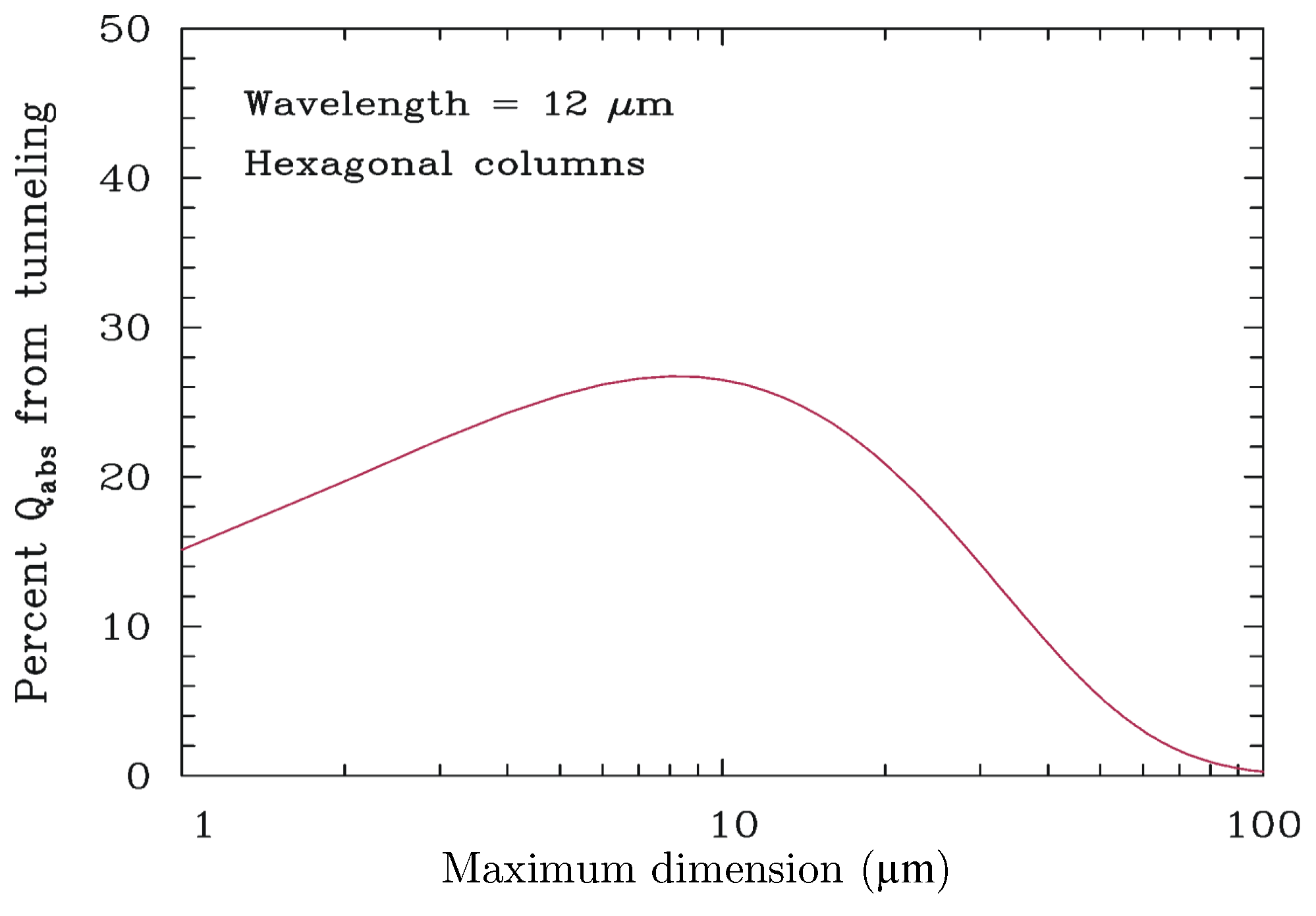
Figure 1Percent contribution of wave resonance absorption to the overall absorption efficiency at 12 µm wavelength as a function of maximum dimension D for hexagonal columns, as estimated by the MADA. It is decreasing to below 10 % of its maximum for sizes larger than about 60 µm.
In this study, we use CALIPSO IIR channels at 12.05 and 10.6 µm. Since mi at 10.6 µm is less than mi at 11 µm, some Beer's law type absorption may contribute to absorption differences between the 10.6 and 12 µm channels when PSD are sufficiently narrow. This acts to slightly extend the dynamic range of sensitivity relative to the 11–12 µm channel combination.
2.2 Retrieving βeff from IIR and CALIOP observations
We use the absorption optical depth τabs(12.05 µm) and τabs(10.6 µm) retrieved from the effective emissivity in CALIPSO IIR channels 12.05 and 10.6 µm. The retrieved optical depths are not purely due to absorption, but also include the effects of scattering. Thus, their ratio is not exactly β, but is the effective β or βeff written as
IIR βeff is based on the CALIPSO IIR Version 3 Level 2 track product (Vaughan et al., 2017). This product includes a scene typing built from the CALIOP Version 3 5 km cloud and aerosol layer products. The scene classification has been refined for this study to account for additional dense clouds in the planetary boundary layer reported in the CALIOP Version 3 333 m layer product. The methodology for retrieving IIR effective emissivity and βeff from co-located CALIOP observations and IIR radiances is detailed in Garnier et al. (2012, 2013). IIR effective emissivity was reprocessed for this study to reduce possible biases, as described in the following sub-sections. Version 3 CALIOP cloud extinction coefficient profiles are used for some of the corrections. IIR calibrated radiances are from the recently released Version 2 Level 1b products (Garnier et al., 2018). These improvements will be implemented in the next Version 4 of the IIR Level 2 products. This is why we only focus in this study on a limited data set as a proof-of-concept. We will further develop a more statistically relevant analysis using the Version 4 products.
For each IIR channel, τabs is derived from the effective emissivity, ε, as
with
where Rm is the measured calibrated radiance, RBB is the opaque (i.e., blackbody) cloud radiance, and RBG is the background radiance that would be observed in the absence of the studied cloud, as described in Garnier et al. (2012).
The cloud effective emissivity ε and the subsequent βeff are retrieved for carefully selected cirrus clouds, as described in Sect. 2.2.1. The retrievals are cloud layer average quantities as seen from space, whose representative altitude and temperature are estimated using additional information from CALIOP vertical profiling in the cloud, as presented in Sect. 2.2.3. As such, they can differ from in situ local measurements in the cloud.
2.2.1 Cloud selection
Because IIR is a passive instrument, meaningful retrievals are possible for well identified scenes. This study is restricted to the cases where the atmospheric column contains one cirrus cloud layer. We also ensure that the background radiance is only due to the surface (see Eq. 3) allowing a more accurate computation than for cloudy scenes. The retrievals were applied only to single-layered semi-transparent cirrus clouds that do not fully attenuate the CALIOP laser beam, so that the cloud base is detected by the lidar. The cloud base is in the troposphere and its temperature is required to be colder than −38 ∘C (235 K) to ensure that the cloud is entirely composed of ice. This is likely to exclude liquid-origin cirrus clouds from our data set (Luebke et al., 2016). When the column also contains a dense water cloud, the background radiance can be computed assuming that the water cloud is a blackbody. However, because systematic biases were made evident (Garnier et al., 2012), we chose to discard these cases, which reduces the number of selected samples by about 25 %. Because the relative uncertainties in τabs and in βeff increase very rapidly as cloud emissivity decreases (Garnier et al., 2013), the lidar layer-integrated attenuated backscatter (IAB) was chosen greater than 0.01 sr−1 to avoid very large uncertainties at the smallest visible optical depths (ODs). This resulted in an OD range of about 0.3 to 3.0. Similarly, clouds for which the radiative contrast RBG−RBB between the surface and the cloud is less than 20 K in brightness temperature units are discarded. IIR observations must be of good quality according to the quality flag reported in the IIR Level 2 product (Vaughan et al., 2017).
2.2.2 Background radiance, RBG
The brightness temperature TBG associated to the clear sky background radiance RBG is derived from the Fast Radiative (FASTRAD) transfer model (Dubuisson et al., 2005) fed by atmospheric profiles and skin temperatures from GMAO GEOS5, along with pre-defined surface emissivities inferred from the International Geosphere and Biosphere Program (IGBP) surface types and a daily updated snow and ice index (Garnier et al., 2012). For this study, remaining biases at 12.05 and 10.6 µm between observations and the FASTRAD model are corrected using monthly maps of mean differences between observed and computed brightness temperatures (called BTDoc) in clear sky conditions. The corrections are applied over ocean and over land with a resolution of 2∘ in latitude and 4∘ in longitude, by separating daytime and nighttime data. Figures S1a and S1b in the Supplement show distributions of BTDoc before and after correction. After correction, BTDoc is equal to zero on average for both channels.
2.2.3 Blackbody radiance, RBB
In Version 3 IIR products, RBB (and the associated blackbody temperature TBB) is derived from the cloud temperature, Tcaliop, evaluated at the centroid altitude of the CALIOP 532 nm attenuated backscatter profile using GMAO GEOS5 temperature (Garnier et al, 2012). In this study, a correction is further applied using CALIOP extinction profiles in the cloud layer as described in Sect. 3 of Garnier et al. (2015). The CALIOP lidar 532 nm extinction profile in the cloud is used to determine an IIR weighting profile that is used, together with the GMAO GEOS5 temperature profile, to compute RBB as the weighted averaged blackbody radiance. The lidar vertical resolution is 60 m, and emissivity is weighted in a similar way with the 532 nm extinction profile. The weight of each 60 m bin is its emissivity at 12.05 µm attenuated by the overlying infrared absorption optical depth, normalized to the cloud emissivity. Computing TBB at 10.6 and at 12.05 µm yields temperatures that differ by less than 0.15 K on average, which has a negligible impact on βeff for our cloud selection.
In addition, the altitude and temperature associated to the layer average βeff are characterized using the centroid altitude, Zc, and centroid temperature, Tc, of the IIR weighting profile. Note that Tc and TBB are not identical, but typically differ by less than a few tenths of a Kelvin.
2.2.4 Estimated uncertainties in βeff
The uncertainty in βeff, Δβeff, is computed by propagating the errors in τabs(12.05 µm) and τabs(10.6 µm). These errors are themselves computed by propagating the errors in (i) the measured brightness temperatures Tm associated to Rm, (ii) the blackbody brightness temperature TBB, and (iii) the background brightness temperatures TBG (Garnier et al., 2015). The uncertainties in Tm at 10.6 and 12.05 µm are random errors set to 0.3 K according to the IIR performance assessment established by the Centre National d'Etudes Spatiales (CNES) assuming no systematic bias in the calibration. They are assumed to be statistically independent. In contrast, the error in TBB is the same for both channels, because the same cloud temperature TBB is used to compute τabs(12.05 µm) and τabs(10.6 µm). A random error of ±2 K in TBB is estimated to include errors in the atmospheric model. After correction for systematic biases based on differences between observations and computations in cloud-free conditions (see Sect. 2.2.2), the error in TBG is considered a random error, which is taken equal to the standard deviation of the corrected distributions of BTDoc (Fig. S1a). As a result, the uncertainty in TBG at 12.05 µm is set to ±1 K over ocean, and to ±3 K over land for both night and day. Standard deviations of the distributions of [BTDoc(10.6 µm)–BTDoc(12.05 µm)] are generally smaller than 0.5 K (Fig. S1b). Accounting for the contribution from the measurements, which is estimated to be K, this indicates that the biases in TBG at 10.6 and at 12.05 µm are nearly canceling out and can therefore be considered identical. More details about the uncertainty analysis can be found in the appendix.
The relative uncertainty Δβeff∕βeff is mostly due to random measurement errors, because systematic biases associated with the retrieval of τabs(12.05 µm) and τabs(10.6 µm) tend to cancel when these are ratioed to calculate βeff.
2.3 Relating βeff to N∕IWC and De based on aircraft PSD measurements
Using aircraft data from the DOE ARM supported Small Particles in Cirrus (SPARTICUS) field campaign in the central United States (Jensen et al., 2013a) and the NASA supported Tropical Composition, Cloud and Climate Coupling (TC4) field campaign near Costa Rica (Toon et al., 2010), βeff was related to cirrus cloud microphysical properties. The SPARTICUS field campaign, conducted from January through June 2010 in the central United States (for domain size, see Fig. 2 in Mishra et al., 2014), was designed to better quantify the concentrations of small (D<100 µm) ice crystals in cirrus clouds. Regarding SPARTICUS, the data set described in Mishra et al. (2014) was used, and the TC4 data are described in Mitchell et al. (2011b). Details regarding field measurements, the flights analyzed and the microphysical processing are described in these articles. PSD sampling times during TC4 were often much longer than for SPARTICUS (<2 min), with mean TC4 sampling times for horizontal legs within aged anvils being 10.56 min (Lawson et al., 2010; Mitchell et al., 2011b). This, along with more in-cloud flight hours during SPARTICUS, resulted in fewer PSD samples for TC4 relative to SPARTICUS. The PSDs were measured by the 2D-S probe (Lawson et al., 2006a, 2011) where ice-particle concentrations were measured down to 10 µm (5–15 µm size bin) and up to 1280 µm in ice-particle length (when using “all-in” data processing criteria). βeff was calculated from these PSDs using the method described in Parol et al. (1991) and Mitchell et al. (2010). This method was tested in Garnier et al. (2013, Fig. 1b) where βeff calculated from a radiative transfer model (FASDOM; Dubuisson et al., 2005) was compared with βeff calculated analytically via Parol et al. (1991), with good agreement found between these two methods. More specifically, to calculate βeff from PSD in this study, the PSD absorption efficiency is given as , where βabs is the PSD absorption coefficient (determined by MADA from measured PSD) and APSD is the measured PSD projected area. The PSD effective diameter was determined from the measured PSD as described in Mishra et al. (2014), but in essence is given as , where ρi is the density of bulk ice (0.917 g cm−3). The PSD extinction efficiency was determined in a manner analogous to . The single scattering albedo ωo was calculated as and the PSD asymmetry parameter g was obtained from De using the parameterization of Yang et al. (2005). Knowing , ωo and g, βeff was calculated from the PSD as follows:
Note that β (i.e., βeff without scattering effects) is equal to .

Figure 2Dependence of N∕IWC (g−1) on the effective absorption optical depth ratio βeff as predicted from the method of Parol et al. (1991), based on PSDs from SPARTICUS synoptic cirrus (blue squares) and anvils (black squares), and TC4 aged (red diamonds) and fresh (black diamonds) anvils, where the first size bin is included. The larger (smaller) symbols denote PSDs measured at a temperature colder (warmer) than −38 ∘C. The curve-fit equations are for SPARTICUS synoptic cirrus (blue) and for TC4 aged and fresh anvils (red).
Figure 2 shows measurements of N∕IWC from SPARTICUS flights over the central United States, based on PSD sampled from synoptic (blue squares) and anvil (black squares) cirrus clouds. Cirrus cloud PSD were measured using the 2D-S probe, which produces shadowgraph images with true 10 µm pixel resolution at aircraft speeds up to 170 m s−1, measuring ice particles between 10 and 1280 µm (or more) (Lawson et al., 2006a, 2011). The 2D-S PSD data were post-processed using an ice-particle arrival time algorithm that identifies and removes ice shattering events from the data stream. All size bins of the 2D-S probe were used here. Two SPARTICUS flights from 28 April were added to this synoptic data set (giving a total of 15 flights) as 28 April was previously mislabeled as an anvil cirrus case study, but was actually a ridge-crest cirrus event (a type of synoptic cirrus) as described in Muhlbauer et al. (2014). This “ridge crest cirrus” had high N (500–2200 L−1) for ∘C. Also shown are N∕IWC measurements from the TC4 field campaign for maritime “fresh” (black diamonds) anvil cirrus (during active deep convection where the anvil is linked to the convective column) and for aged (red diamonds) anvil cirrus (anvils detached from convective column). Figure 2 relates βeff to the N∕IWC ratio, where βeff was calculated from the same PSD measurements used to calculate N and IWC, based on the MADA method. The PSD measurements include size-resolved estimates of ice-particle mass concentration based on Baker and Lawson (2006a), size-resolved measurements of ice projected area concentration and the size resolved number concentration. This PSD information is the input for the MADA method that yields the coefficients of absorption and extinction. The wave resonance efficiency Re used in MADA was estimated from Table 1 in Mitchell et al. (2006; referred to as tunneling efficiencies), where for , droxtals and hexagonal columns are assumed and Re=0.90; for , budding bullet rosettes and hexagonal columns are assumed and Re=0.50; for D>100 µm, bullet rosettes and aggregates are assumed and Re=0.15. This shape-dependence on ice-particle size was guided by the ice-particle size–shape observations reported in Lawson et al. (2006b), Baker and Lawson (2006b) and Erfani and Mitchell (2016), where small hexagonal columns (for which we can estimate Re) are substituted for small irregular crystals. These ice-particle shape assumptions affect only Re, and the cloud optical properties are primarily determined through the PSD measurements noted above (i.e., not the value of Re). Due to βeff's sensitivity to wave resonance and small ice crystals, a tight and useful relationship is found between N∕IWC and βeff for g−1 for both campaigns. As far as we know, this relationship was not known previously. The associated PSDs were measured at temperatures colder than −38 ∘C (large symbols), which is the cloud base temperature of the cirrus clouds targeted for this study. For g−1, βeff reaches a low limit and is not sensitive to N∕IWC, so that N∕IWC cannot be estimated from βeff. Much of the data with βeff reaching the “no sensitivity” low limit were derived from ice cloud PSDs at temperatures between −20 and −38 ∘C (small symbols) where PSD tend to be relatively broad.
Table 1Regression curve variables and coefficients for second-order polynomials of the form , used in the CALIPSO retrieval. Units for N∕IWC and De are in g−1 and microns, respectively.
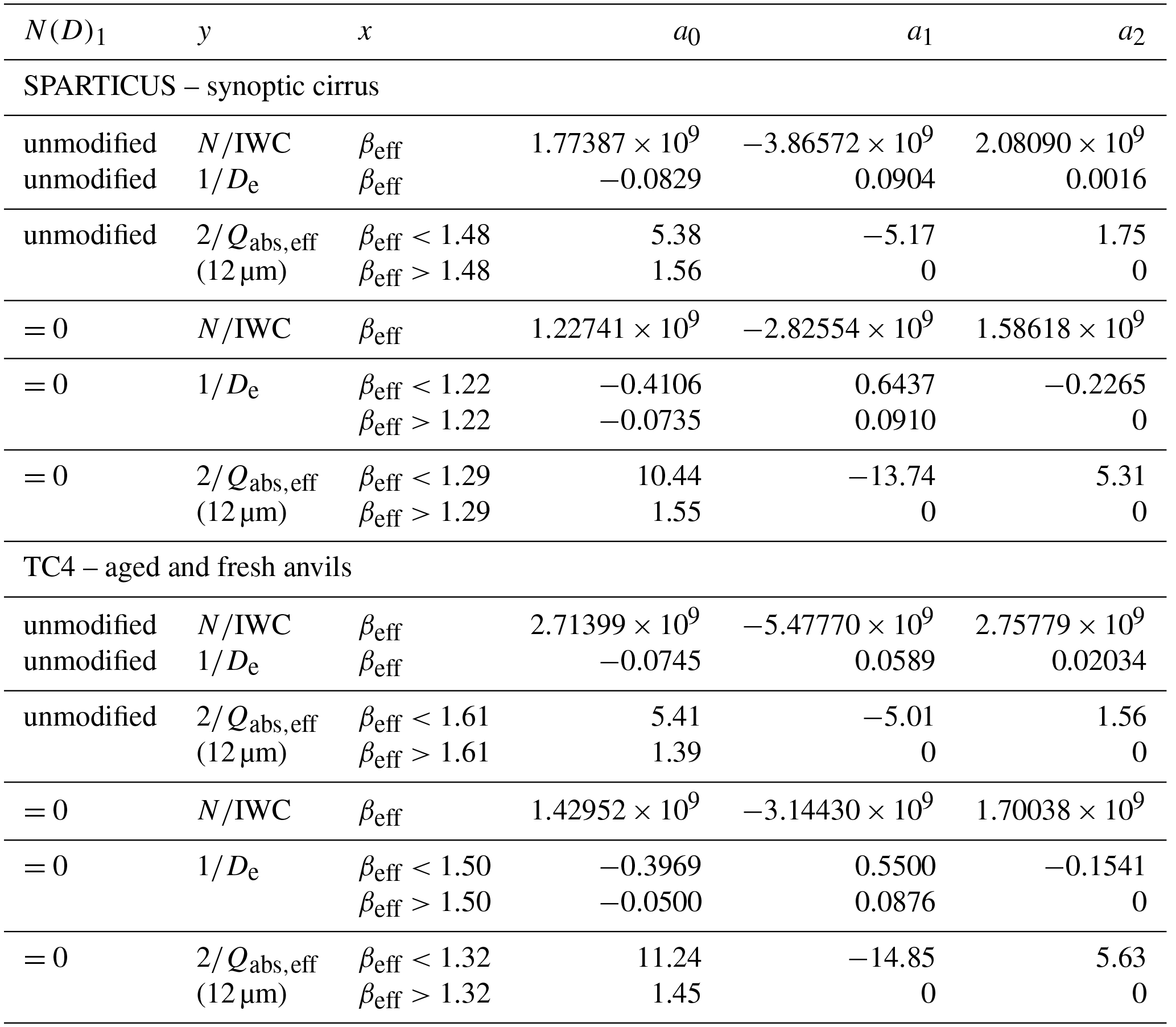
N(D)1 unmodified: SPARTICUS: if βeff<1.031,
then x=1.031; TC4: if βeff<1.04085, then
x=1.04085.
N(D)1=0: SPARTICUS: if βeff<1.03078, then
x=1.03078; TC4: if βeff<1.04410, then x=1.04410.
Because the clouds selected in this study are single-layered semi-transparent cirrus clouds, the relationships seen for synoptic cirrus during SPARTICUS could be deemed the most relevant for this study. But interestingly, synoptic and anvil cirrus during SPARTICUS (squares) follow similar relationships, and similarly, aged and fresh cirrus anvils (diamonds) follow similar relationships during TC4. Thus, the fact that anvil and synoptic cirrus during SPARTICUS follow a similar relationship suggests that the relationship established from anvils during TC4 could also be relevant for this study. The blue line shows the curve fit derived from SPARTICUS synoptic cirrus, while the red line is derived from aged and fresh anvils during TC4. The blue and the red lines are similar for the largest βeff (βeff>1.2) and progressively depart as βeff decreases. The βeff low limit is 1.031 during SPARTICUS, for both synoptic and anvil cirrus, whereas it is 1.041 during TC4. The different βeff low limits during SPARTICUS and TC4 may reflect different PSD shapes measured during these two campaigns. This indicates that as βeff decreases and its sensitivity to N∕IWC decreases, the sensitivity of the relationships to the PSD increases. These two curves are indicative of the possible dispersion in the relationships, and therefore will both be considered in the analysis.
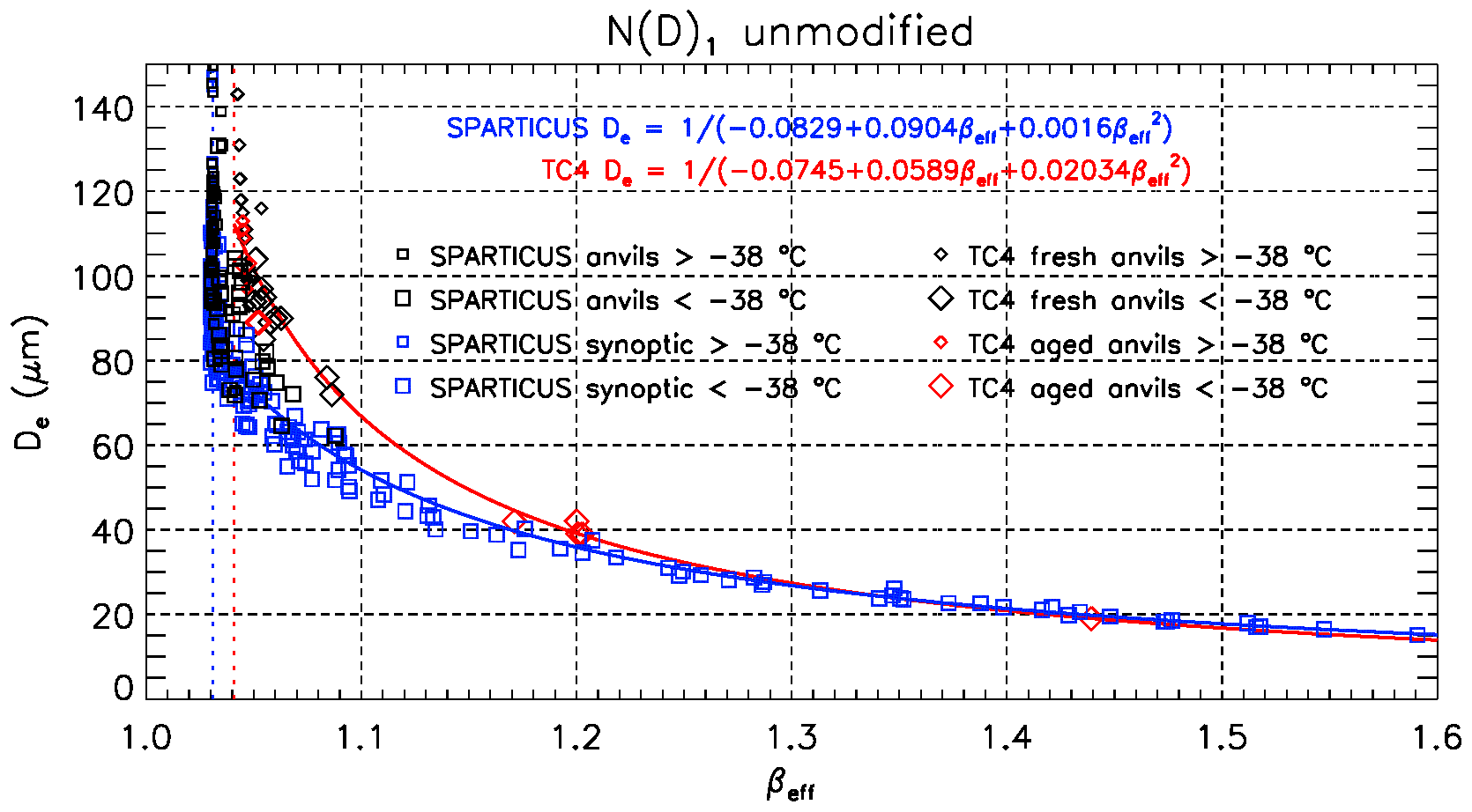
Figure 3Dependence of the PSD effective diameter De (µm) on the effective absorption optical depth ratio βeff as predicted from the method of Parol et al. (1991), based on PSDs from SPARTICUS synoptic cirrus (blue squares) and anvils (black squares), and TC4 aged (red diamonds) and fresh (black diamonds) anvils, where the first size bin is included (N(D)1 unmodified). The larger (smaller) symbols denote PSDs measured at a temperature colder (warmer) than −38 ∘C. The curve-fit equations give 1∕De in µm−1; they are for SPARTICUS synoptic cirrus (blue) and for TC4 aged and fresh anvils (red).
Using this same in situ data and methodology, βeff has also been related to De as shown in Fig. 3, where all PSD bins were used. De is defined as (3/2) IWC∕(ρiAPSD) where ρi is the density of bulk ice (Mitchell, 2002). Accordingly, De was calculated from the measured PSD (see Mishra et al., 2014). The relationships derived from SPARTICUS synoptic cirrus and from TC4 anvils are shown in blue and red, respectively. They are only useful for De<90 or De<110 µm, respectively, since βeff is only sensitive to the smaller ice particles. The relationships are similar for De below 30 µm. This emphasizes the fact that βeff is a measure of the relative concentration of small ice crystals in a PSD (Mitchell et al., 2010). APSD and βeff (PSD integrated quantities) may be associated with a substantial portion of larger ice particles (D>50 µm) before βeff loses sensitivity to changes in De. There are much fewer TC4 points in Figs. 2 and 3 for βeff>1.1 since the higher βeff values were obtained only for ∘C, which only occurred during two SPARTICUS flights on 28 April.
Cirrus cloud emissivity and τabs depend on ice-particle shape (Mitchell et al., 1996a; Dubuisson et al., 2008). However, two factors may reduce the dependence of this retrieval on ice-particle shape, one being that βeff is directly retrieved from cloud radiances as per Eqs. (2) and (3). Another reason is that no ice-particle shape assumptions are made when calculating βeff from in situ measurements with the exception of the absorption contribution from wave resonance (which was not sensitive to realistic shape changes, as described in Sect. 2.4). That is, the 2D-S probe in situ data include measurements and estimates for ice-particle projected area and mass, respectively, as noted above. MADA optical properties are calculated directly from these in situ area and mass values, thus largely avoiding the need for shape assumptions. In addition, this retrieval is most sensitive to the smaller ice particles in a PSD where ice-particle shape is difficult to measure. If certain ice nucleation mechanisms and environmental conditions promote some types of ice embryos over others (e.g., quasi-spherical vs. hexagonal columns/plates), there may be some dependence on ice crystal shape. An analysis of small ice crystal shapes in cirrus clouds can be found in Baker and Lawson (2006b), Lawson et al. (2006b) and Woods et al. (2018). During the SPARTICUS campaign, many cirrus clouds were sampled so that biases in ice-particle shape are less likely to occur.
2.4 Impact of the smallest size bin in PSD measurements
The relationships shown in Figs. 2 and 3 were derived by using all the size bins of the 2D-S probe. However, the data in the smallest size bin (5–15 µm) has the greatest uncertainty since the sample volume of the 2D-S probe depends on particle size, and this volume is smallest (with greatest measurement uncertainty) for the smallest size bin (Gurganus and Lawson, 2018). This motivated us to formulate the retrieval relationships in two ways: (1) by assuming that the PSD first size bin, N(D)1, is valid and is therefore unmodified (as considered earlier), and (2) by assuming that N(D)1 equals zero. Physical reasons to argue in favor of the unmodified N(D)1 assumption or the N(D)1=0 assumption are discussed in the Supplement.
Figure S2 in the Supplement shows the N∕IWC-βeff and De-βeff relationships derived from SPARTICUS and TC4 assuming N(D)1=0. Assuming N(D)1=0 not only reduces N, but it also reduces βeff especially when βeff is large. For instance, assuming N(D)1=0 reduces the maximum value of in situ βeff from 1.6 to 1.24 during SPARTICUS, and from 1.44 to 1.27 during TC4. As a result, the relationships are fairly close for both assumptions. For example, assuming N(D)1=0 reduces N∕IWC by about 20 % for the largest βeff, thereby confirming the tight relationship between N∕IWC and βeff shown in Fig. 2. Assuming N(D)1=0 has a larger impact on the De–βeff relationship, as shown in Fig. S2. For SPARTICUS, the largest relative change in De is around βeff=1.15, where De is reduced by 26 % assuming N(D)1=0 instead of N(D)1 unmodified. For TC4, the largest relative reduction in De is 38 % at βeff=1.2. It is noted that the De–βeff relationships used in the IIR Version 3 operational algorithm (Fig. 3a in Garnier et al., 2013) tend to yield smaller De than the relationships derived from these PSD measurements, largely because they were computed with no size distribution.
The unmodified N(D)1 assumption can be viewed as an upper limit while the N(D)1=0 assumption is clearly a lower limit for the actual value of N(D)1, and in this way our relationships are bracketed by these two limiting conditions. The comparison of in situ βeff for each of these assumptions with βeff derived independently from CALIPSO IIR is an additional piece of information, as discussed in Sect. 4.
Uncertainties regarding the wave resonance efficiency (Re) values assumed in Sect. 2.3 were evaluated, but these were much smaller than the uncertainties described above. For example, assuming bullet rosettes for all sizes results in Re values of 0.70, 0.40 and 0.15 for the three size categories considered (from smallest to largest). Among plausible crystal shape assumptions, this assumption yielded the lowest Re values, reducing βeff by no more than 2.6 %. Note that for D<80 µm, more than 85 % of the ice particles tend to be irregular (e.g., blocky or quasi-spherical) or spheroidal in shape (Lawson et al., 2006b; Baker and Lawson, 2006b), and these shapes should correspond to relatively high Re values (Mitchell et al., 2006).
2.5 Retrieving N from CALIPSO βeff
Using cloud layer average βeff derived from IIR and CALIOP observations (Sect. 2.2), the N∕IWC-βeff- and De-βeff relationships established from in situ measurements (Sects. 2.3 and 2.4) are used to derive the cloud layer N from CALIPSO, as presented in this sub-section. The sensitivity ranges ( g−1 & De<90–110 µm) are usually compatible with cirrus clouds ( ∘C) since PSDs tend to be narrower at these temperatures, containing relatively small ice particles (e.g., Mishra et al., 2014). Contrasting the SPARTICUS and TC4 relationships for both N(D)1 assumptions provides a means of estimating the uncertainty in N resulting from regional differences in cirrus microphysics.
Using CALIPSO βeff and the N∕IWC-βeff and De-βeff relationships, the cloud layer N is retrieved as with IWC computed as follows:
where ρi is the bulk density of ice (0.917 g cm−3), and αext is the effective layer-average visible extinction coefficient, which is derived from CALIOP and IIR as follows:
The quantity (12 µm), where 2 is the value of for ice PSDs in the visible spectrum, converts τabs(12.05 µm) to an equivalent visible extinction optical depth (OD). It is obtained from βeff as illustrated in Fig. 4 for the unmodified N(D)1 assumption, and for the N(D)1=0 assumption in Fig. S3 (in the Supplement). For a given βeff, (12 µm) is smaller by less than 7 % assuming N(D)1=0, and consequently, IIR αext is also smaller by less than 7 %. The effective cloud thickness, Δzeq, accounts for the fact that the IIR instrument does not equally sense all of the cloud profile that contributes to thermal emission. This is accounted for through the IIR weighting profile introduced in Sect. 2.2.3, which gives more weight to large emissivity and therefore to the large extinctions in the cloud profile. Using the IIR weighting profile, the layer absorption coefficient αabs(12.05 µm) for the IIR 12.05 µm channel is computed from the weighted averaged absorption coefficient profile. This yields αabs(12.05 µm) > αabs,mean(12.05 µm), where αabs,mean(12.05 µm) is the mean absorption coefficient, that is, the ratio of τabs(12.05 µm) to the CALIOP layer geometric thickness, Δz. Thus, an equivalent effective thickness is defined as Δzeq where , or alternatively, Δzeq=Δz (). In practice, Δzeq is found to be equal to 30 % to 90 % of Δz.
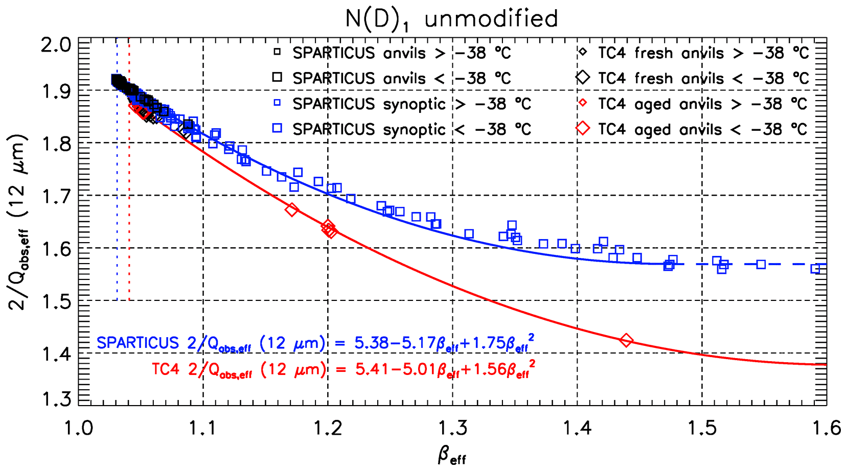
Figure 4The βeff dependence of the term that converts the absorption optical depth τabs into visible optical depth in Eq. (7), based on PSDs from SPARTICUS synoptic cirrus (blue squares) and anvils (black squares), and TC4 aged (red diamonds) and fresh (black diamonds) anvils, where the first size bin is included (N(D)1 unmodified). The larger (smaller) symbols denote PSDs measured at a temperature colder (warmer) than −38 ∘C. The curve-fit equations are for SPARTICUS synoptic cirrus (blue) and for TC4 aged and fresh anvils (red). The dashed lines are where the curve-fit equations are extrapolated (see Table 1).
To summarize, the retrieval equation is as follows:
The retrieval of τabs(12.05 µm) and τabs(10.6 µm) combined with the CALIOP extinction profile provides βeff, N∕IWC, De, αext, and therefore layer-average IWC and finally layer N. Perhaps the most unique aspect of this retrieval method is its sensitivity to small ice crystals via βeff.
3.1 Regression curves
Regression curves derived from SPARTICUS and TC4 for both assumptions [N(D)1 is unmodified and N(D)1=0] for the quantities N∕IWC, De and (12 µm) are given in Table 1, constituting the four formulations of this retrieval scheme. A number of adjustments of the second-order polynomials were needed to provide retrievals for any value of βeff. They correspond to the dashed lines in Fig. 4 (blue), Fig. S2 (bottom) and in Fig. S3.
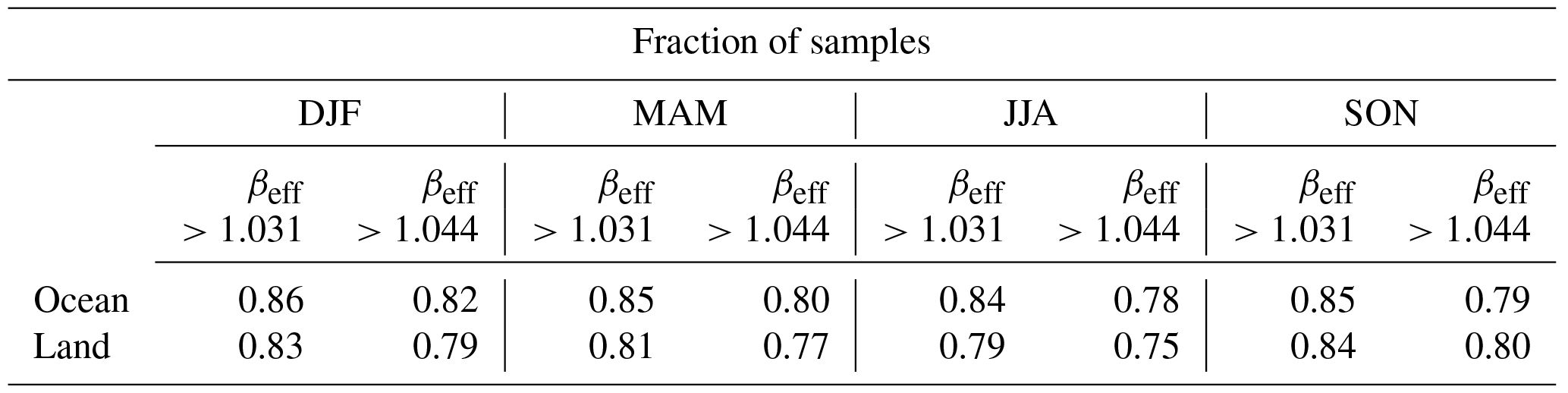
When calculating N∕IWC, De and (12 µm) from βeff, if the retrieved βeff is less than the lower sensitivity limit, then βeff is set to this value. For instance, N∕IWC corresponding to this value via the regression curves is about 2.3×10⁵ g−1. As shown in Table 2 for the year 2013, this practice affected 15 % and 18 % of the N∕IWC and De retrievals over ocean and land, respectively, when using the SPARTICUS relationships, for which the lower sensitivity limit is βeff=1.031. Using the TC4 relationships, 20 % and 22 % of the samples over ocean and land, respectively, had βeff smaller than the sensitivity limit of 1.044. To better estimate the median values and percentiles for N and De, N and De retrievals calculated using these limiting values are accounted for when determining these statistics.
Table 2Fraction of samples with IIR βeff larger than the N∕IWC and De sensitivity limit, per season in 2013, over ocean and over land.
The retrieved N for the four formulations of the retrieval scheme can be compared through the product of the three βeff-dependent quantities, N∕IWC, De and (12 µm), as shown in Fig. 5. The upper and lower bounds are the SPARTICUS N(D)1 unmodified and TC4 N(D)1=0 formulations, which differ by about a factor of 2 in retrieved N for βeff>1.06, and by up to a factor of 10 when βeff is between the SPARTICUS (1.031) and TC4 (1.044) sensitivity limits.
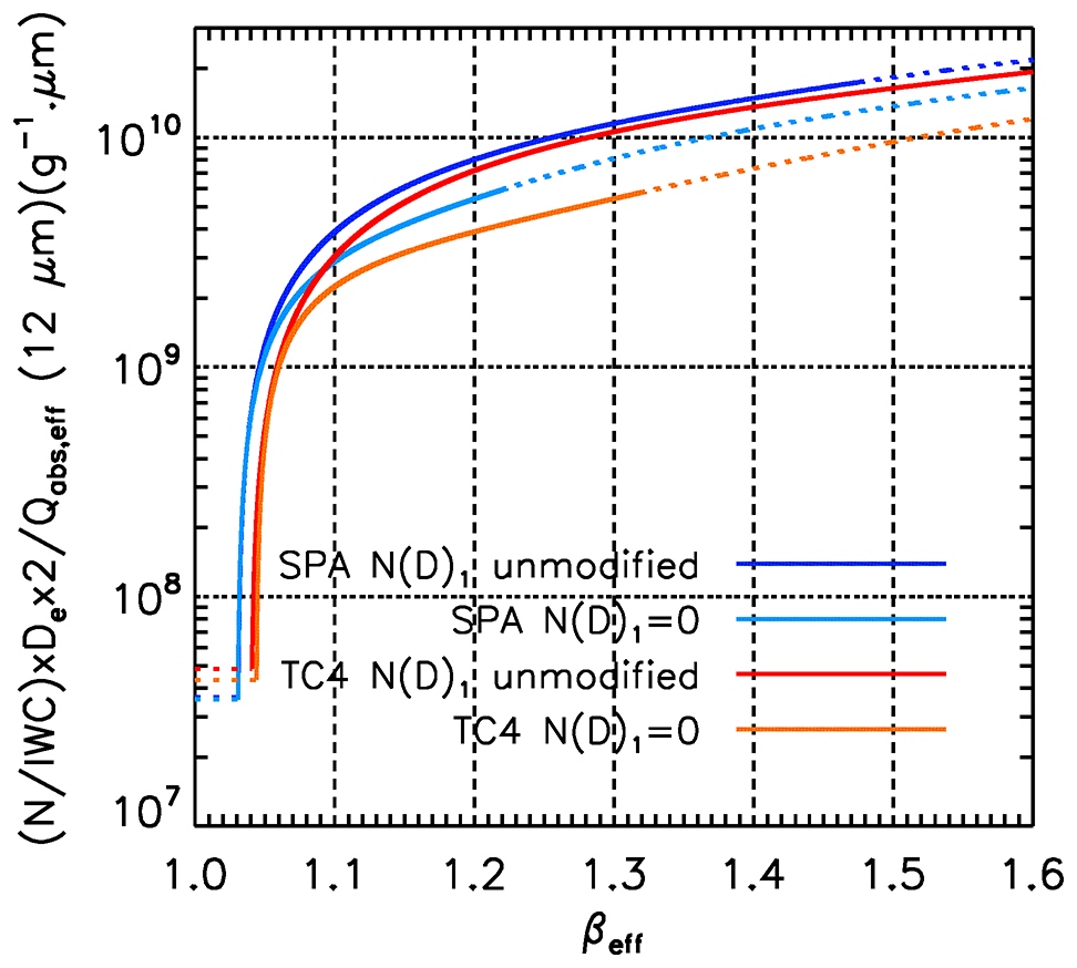
Figure 5Comparison of ice-particle number concentration N derived from CALIPSO βeff using the four formulations of the retrieval scheme, derived from SPARTICUS using the N(D)1 unmodified (navy blue) and N(D)1=0 (light blue) assumptions, and from TC4 using the unmodified (red) and N(D)1=0 (orange) assumptions. The dashed lines are where the curve-fit equations are extrapolated (see Sect. 3 and Table 1).
3.2 Retrieval uncertainties
The inter-relationship between βeff and αext, IWC, and N is illustrated in the Supplement under “Relationship between βeff, αext, IWC and N”, and in Figs. S4 and S5. After re-writing Eq. (8) as a function of βeff and τabs(12.05 µm) using the regression curves shown in Fig. 5, the uncertainty ΔN is computed by propagating the errors in βeff (see Sect. 2.2.4) and in τabs(12.05 µm), assuming a negligible error in ΔZeq (Eq. 7) and in the relationships. Errors in the relationships create additional systematic uncertainties, as discussed in Sect. 3.1. More details about the uncertainty analysis and the equations used to compute ΔN can be found in the Appendix.
Figure S4 (bottom row) shows ΔN∕N against βeff for the same samples as in the top row of Fig. S4. ΔN∕N decreases as βeff increases, reflecting that the technique is sensitive to small crystals. ΔN∕N is found most of the time <0.50 for βeff>1.15, but increases up to more than 2.0 as βeff decreases and approaches the sensitivity limit. For a given value of βeff, the variability of ΔN∕N is due to the variability of Δβeff∕βeff and of Δαext∕αext. ΔN∕N is larger over land because of a larger estimated uncertainty in TBG and also because the radiative contrast is sometimes relatively weak. Δβeff∕βeff is mostly due to random measurement errors, because systematic errors associated with the retrieval of τabs(12.05 µm) and τabs(10.6 µm) tend to cancel when these are ratioed to calculate βeff. The uncertainty in TBG contributes more importantly to Δαext∕αext at the smallest emissivities. Uncertainty in TBB is not a major contributor for semi-transparent clouds of small to medium emissivity.
We repeated this analysis except using an OD threshold of 0.1 (instead of 0.3; see also Sect. 5.1). Figure S5 shows this same analysis except that the sample selection criteria for minimum OD was changed from 0.30 to 0.10. In the lower row relating ΔN∕N to βeff, the number of samples that have has substantially increased over both ocean and land relative to Fig. S4 due to the lower OD threshold for sample selection, and more samples correspond to lower values of αext, IWC, and N.
Because our analysis is applied to IIR βeff using relationships with in situ βeff established from the SPARTICUS and TC4 field campaigns, a quantitative comparison of IIR and in situ βeff from these two campaigns is first discussed. Secondly, retrieved N∕IWC are compared against in situ N∕IWC measured from many field campaigns using the data set of Krämer et al. (2009), where N and IWC are measured independently. The last step of this evaluation is to compare retrieved and in situ De, IWC and N.
4.1 Comparing IIR and in situ βeff during SPARTICUS and TC4 – Impact of the smallest size bin in PSD measurements
For SPARTICUS, the CALIPSO retrievals were restricted to the relevant domain (latitude range 31–42∘ N and longitude range 90–103∘ W) and they were obtained from January through April 2010 during daytime since this period contained only synoptic cirrus based on the SPARTICUS flights. For TC4, the CALIPSO retrievals were restricted to the TC4 spatial and temporal domain (latitude range 5∘ S–15∘ N and longitude range 80–90∘ W) over oceans, in July and August 2007. CALIPSO retrievals are cloud layer average properties, and we use Tc (see Sect. 2.2.3) as our best characterization of the representative cloud temperature. Finally, for each campaign, in situ βeff is computed for both N(D)1 assumptions. Data analysis is performed on a statistical basis, as coincident in situ and satellite data only provide a very small data set due to our data selection.
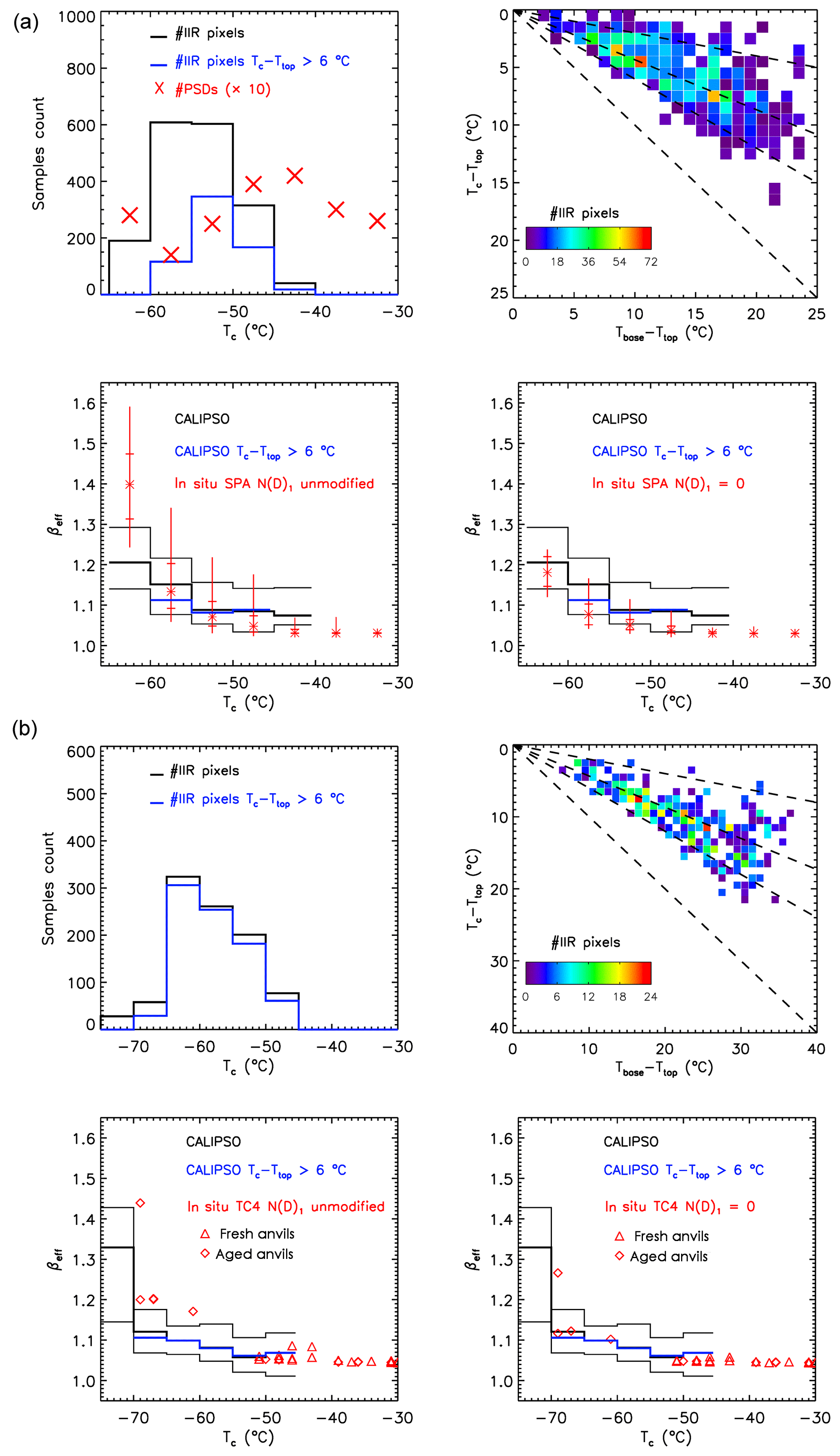
Figure 6(a) Statistical comparison of CALIPSO IIR βeff and in situ βeff (synoptic cirrus) during SPARTICUS (sampled January–April 2010). Top left: the red X symbols indicate the number of PSDs used in the SPARTICUS analysis (multiplied by 10 for clarity of presentation) within 5 ∘C in situ temperature intervals, while the black histogram indicates the number of CALIPSO IIR pixels in each Tc temperature interval, and the blue histogram indicates the number of IIR pixels where Tc−Ttop is larger than 6 ∘C. Top right: 2D-histograms of Tc−Ttop and Tbase−Ttop for the IIR pixels. The dashed lines from top to bottom are 20 %, 43 % (average value) and 60 % from cloud top, with Tc=Tbase for the lowest curve. Bottom: temperature dependence of in situ βeff derived assuming N(D)1 unmodified (left) and N(D)1=0 (right). The vertical lines give the measurement range, the horizontal bars give the 25th and 75th percentile values, and the asterisks give the median value. CALIPSO IIR median βeff is given by the thick black histogram, with thin black histograms giving the 25th and 75th percentile values. The thick blue histogram is CALIPSO IIR median βeff where ∘C. (b) Statistical comparison of CALIPSO IIR βeff and in situ βeff during TC4. Top left: the black histogram indicates the number of CALIPSO IIR pixels in each Tc temperature interval, and the blue histogram indicates the number of IIR pixels where Tc−Ttop is larger than 6 ∘C. Top right: 2D-histograms of Tc−Ttop and Tbase−Ttop for the IIR pixels. The dashed lines from top to bottom are 20 %, 43 % and 60 % from cloud top, with Tc=Tbase for the lowest curve, for comparison with SPARTICUS data. Bottom: temperature dependence of in situ βeff derived assuming N(D)1 unmodified (left) and N(D)1=0 (right) for fresh (red triangles) and aged (red diamonds) anvils. CALIPSO IIR median βeff is given by the thick black histogram, with thin black histograms giving the 25th and 75th percentile values. The thick blue histogram is CALIPSO IIR median βeff where ∘C.
Comparisons with SPARTICUS are reported in Fig. 6a. The upper left panel shows the number of IIR pixels and in situ PSDs per 5 ∘C temperature-bin. As seen in the upper right panel of Fig. 6a, the difference between the temperatures at cloud base (Tbase) and cloud top (Ttop) is smaller than 20 ∘C for most of the clouds selected in the CALIPSO retrievals. Furthermore, Tc tends to be located in the upper part of the cloud layer, at 20 % to 60 % from the top, and on average at 43 %, where the maximum number of IIR observations are found (see dashed black lines). This means that IIR βeff is a weighted measure near the middle of the cloud layer, slightly towards the upper part. A 5 ∘C interval is considered in the analysis in accordance with the dispersion observed in the temperature distributions (Fig. 6a top right). Because IIR pixels are required to correspond to clouds of Tbase less than −38 ∘C, Tc is mostly colder than −45 ∘C, and the number of samples between −45 and −40 ∘C is relatively small (Fig. 6a, upper left panel). It is also seen that Tc−Ttop is smaller than 6 ∘C for the majority of the IIR pixels overall, and for all pixels with ∘C. The temperature dependence of median IIR βeff and of the 25th and 75th percentile values is given by the black histograms in the lower panels of Fig. 6a. The thick blue histogram shows median βeff when Tc−Ttop is larger than 6 ∘C between −60 and −45 ∘C where the number of samples is sufficient (>20) for a meaningful analysis. This smaller median βeff (in blue) illustrates the sensitivity of βeff to distance from cloud top and cloud depth and indicates a smaller fraction of small ice crystals in the PSD for larger distances.
The temperature dependence of IIR βeff is compared with the dependence of in situ βeff derived by taking N(D)1 unmodified (lower left panel) and N(D)1=0 (lower right panel). The red asterisks denote the median in situ values, the red horizontal bars indicate the 25th and 75th percentile values and the vertical red lines indicate the range of values. Median IIR βeff and in situ βeff exhibit a similar temperature variation. A few issues should be kept in mind when interpreting these comparisons. First, regarding the unmodified version of N(D)1 for ∘C, the relatively high median in situ values for βeff and N (ranging from 513 to 2081 L−1) come from two flights on 28 April 2010 that sampled the ridge-crest cirrus mentioned above, raising some concern whether this single cirrus event was representative at these temperatures. A non-representative cirrus event could explain the larger median in situ βeff of 1.4 relative to the median IIR βeff of 1.2 for ∘C. Moreover, N(D)1 for these 28 April PSD samples contributed 78 % of the total N on average. But this would not violate our understanding of cloud physics if the RHi was near 100 %. That is, high N that has very small crystal sizes can exist for long periods when RHi ∼100 % since little ice crystal growth or sublimation can occur then (see Supplement). Second, aircraft sampling at warmer temperatures may not be representative of satellite layer average retrieval at Tc generally located in the upper part of the cloud if the cirrus layer is relatively deep with aircraft sampling relatively low in the cloud. For such conditions, the aircraft sampled ice particles would have relatively long growth times through vapor deposition and aggregation, producing relatively large ice particles and lower βeff and N in the lower cloud. This may have been the case for ∘C. This point is illustrated by the in situ measurements and modeling study of Mitchell et al. (1996b) where a Lagrangian spiral descent through a cirrus layer was simulated with a steady-state snow growth model for vapor deposition and aggregation. Aggregation in the lower cloud was predicted to reduce N by ∼60 %. The larger dispersion of the IIR βeff distribution seen through the difference between the 25th and the 75th percentile values (thin black histograms) can be explained by the uncertainties reported in Table 3.
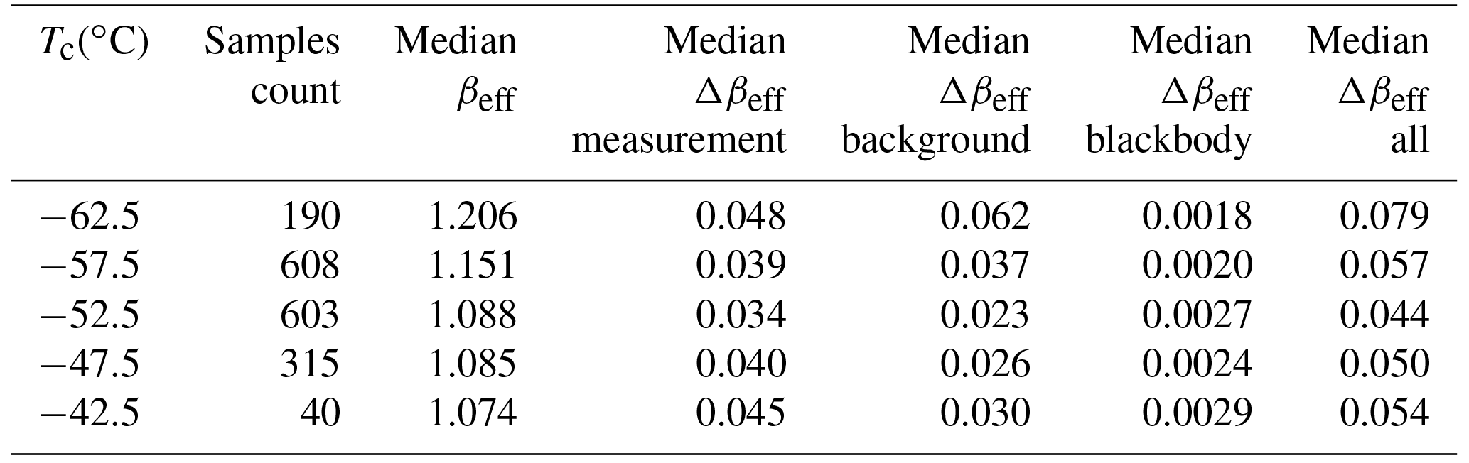
Table 3IIR median βeff (see Fig. 6a) and estimated uncertainty Δβeff during SPARTICUS. See Sect. 2.2.4 and the appendix for details.
Following the same approach as for SPARTICUS, Fig. 6b compares CALIPSO retrievals and TC4 in situ data. The IIR representative temperature is again close to mid-cloud. For temperatures between −69 and −45 ∘C, where CALIPSO and in situ βeff can be compared, most of the CALIPSO selected cirrus clouds have Tc−Ttop larger than 6 ∘C (Fig. 6b, upper left panel) in contrast to SPARTICUS cirrus. The in situ and IIR βeff are in better agreement when in situ βeff is computed without the first size bin (N(D)1=0), especially at the coldest temperatures. The largest in situ βeff at −69 ∘C is in fair agreement with IIR βeff in the neighboring temperature range between −75 and −70 ∘C.
To conclude, we find that despite the a priori different range of cloud optical depths (because TC4 data are from aged and fresh anvils), CALIPSO and in situ βeff are in better agreement for TC4 when the latter are computed using N(D)1=0, most of the time within 0.01–0.02.
4.2 Comparison of N∕IWC with the Krämer cirrus data set
Krämer et al. (2009) compiled coincident in situ measurements of N and IWC from five field campaigns (10 flights) between 68∘ N and 21∘ S latitude where N was measured by the FSSP probe and IWC was directly measured by various probes as described in Schiller et al. (2008). They report mass-weighted ice-particle size Rice derived from in situ measurements of IWC∕N assuming ice spheres at bulk density (0.92 g cm−3). Since Rice can be inverted to yield in situ measurements of N∕IWC, this offers the opportunity to evaluate the representativeness of the four N∕IWC-βeff relationships derived from the SPARTICUS and TC4 campaigns. Krämer et al. (2009) estimated that the FSSP measurements accounted for at least 80 % (but typically >90 %) of the total N in a PSD. These measurements were made at T<240 K where PSD tend to be relatively narrow and ice particle shattering upstream of particle detection (i.e., the sample volume) is less of a problem (de Reus et al., 2009; Lawson et al., 2008). Moreover, the FSSPs used did not use a flow-straightening shroud in front of the inlet; a practice that will reduce the amount of shattering. The complete data set of in situ IWCs reported in Krämer et al. (2009) extends beyond the 10 field campaigns mentioned above, and this complete IWC data set is also described in Schiller et al. (2008).
Since this retrieval is sensitive to the smallest ice crystal sizes, it has the advantage of being sensitive to ice nucleation processes, but this also poses certain challenges. For example, the comparison of retrieved and measured N∕IWC and N in cirrus clouds is necessarily ambiguous due to (1) the uncertainty in PSD probe measurements at the smallest sizes in a PSD (assuming the probe is capable of measuring N between roughly 5 and 50 µm), (2) the PSD size range used to create the retrieval relationships relative to the PSD size range of the measurements used to test the retrieval, (3) the size range of the retrieved PSD (which is unknown), (4) in situ measurements in optically thin layers below the retrieval limit of the IIR for this study, and (5) the comparison of retrieved layer-averaged quantities to localized aircraft measurements, as discussed earlier. Regarding (2), since this retrieval was developed from 2D-S probe in situ measurements, ideally it should be validated against 2D-S probe in situ measurements. Comparing with the Krämer et al. (2009) measurements introduces some ambiguity since the smallest size bin of the 2D-S is from 5 to 15 µm whereas the Krämer et al. (2009) N measurements are based on the FSSP 100/300 that sampled particles in the size range 3.0–30/0.6–40 µm diameter, and ice crystals larger than this size range were not recorded. Moreover, the amount of additional uncertainty in the FSSP measurements due to the possibility of shattering was not quantified. In order to perform the first comparisons, we thus used these in situ measurements of IWC∕N and inferred βeff using the four N∕IWC vs. βeff relationships previously obtained for SPARTICUS and TC4.
The comparisons between the Krämer et al. (2009) in situ values of N∕IWC and the corresponding in situ derived values of βeff (using the four N∕IWC vs. βeff relationships) with the CALIPSO IIR N∕IWC (using these four relationships) and retrieved βeff values are given in Fig. S6 in the Supplement. In situ and IIR N∕IWC values agree rather closely, with IIR N∕IWC having only a weak dependence on the relationship used. Similarly, βeff derived from in situ N∕IWC (using these four relationships) is very consistent with the direct IIR retrieval of βeff for ∘C.
4.3 Comparisons of De, IWC and N with the SPARTICUS, TC4 and Krämer data sets
The in situ and retrieved SPARTICUS cirrus cloud properties, namely De, αext, IWC and N, are shown in Figs. 7a and S7. They are both based on all size bins of the 2D-S probe [N(D)1 unmodified] in Fig. 7a, while these same properties were calculated using the assumption that N(D)1=0 in Fig. S7. The data are presented using the same convention as for βeff in Fig. 6a. For in situ data, the N(D)1 assumption changes mostly N and the smallest De, but has a weaker impact on αext and IWC. For IIR, the changes result from the changes in the relationship with βeff (Figs. 2–5 and S2–S3). Using N(D)1=0 instead of N(D)1 unmodified notably increases the smallest in situ De and always decreases IIR De. The differences between in situ and IIR De increase with temperature as βeff decreases and begins losing sensitivity to De at warmer temperatures. Median in situ and IIR layer average αext, which are both weakly sensitive to the N(D)1 assumption, are within a factor of less than 2. The notable larger variability of the in situ data is explained by the cloud local sampling in contrast to IIR average values. Reflecting the changes in De, IIR IWC is smaller using N(D)1=0. Finally, using N(D)1=0 reduces in situ N by a factor of 3 on average, but the change in the various relationships with βeff is such (Fig. 5) that N derived from IIR βeff is reduced by less than 35 %. The comparison between in situ and layer average IIR N, which is partly driven by the comparison between the respective βeff, is more favorable overall assuming N(D)1 unmodified. The larger median IIR N values at ∘C as compared to the in situ median values is partly due to the fact that IIR βeff is larger than the in situ SPARTICUS low limit of 1.03 and possibly to a larger uncertainty ΔN as βeff approaches the sensitivity limit. As discussed earlier, IIR retrievals are layer average quantities with sensitivity close to the middle part of the cloud layers, whereas in situ measurements can be in the lower or upper part of a relatively deep cloud.
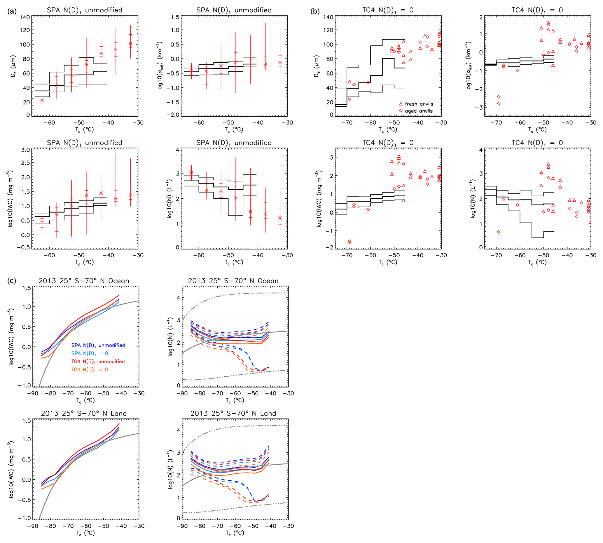
Figure 7(a) SPARTICUS in situ measurements for synoptic cirrus (sampled January–April 2010) are in red, showing the temperature dependence of effective diameter De (µm), extinction coefficient αext (km−1), ice water content IWC (mg m−3) and ice-particle number concentration N (L−1), and correspond to PSD measured within 5 ∘C temperature intervals based on unmodified N(D)1. The vertical lines give the measurement range, the horizontal bars give the 25th and 75th percentile values, and the asterisks give the median value. Corresponding CALIPSO IIR retrieved properties using the SPARTICUS unmodified relationships are given by the thick black histograms, with thin black histograms giving the 25th and 75th percentile values. (b) Temperature dependence of effective diameter De (µm), extinction coefficient αext (km−1), ice water content IWC (mg m−3) and ice-particle number concentration N (L−1) during TC4, based on the N(D)1=0 assumption. In situ TC4 measurements in red are for fresh (triangles) and aged (diamonds) anvils. Corresponding CALIPSO IIR retrieved median properties using the TC4 relationships are given by the thick black histograms, with thin black histograms giving the 25th and 75th percentile values. (c) Left: comparisons of the median CALIPSO IIR IWC (mg m−3) for the four formulations (colored curves) with in situ measurements from Krämer et al. (2009) shown by the grey curve (which is the middle value). Right: comparisons of CALIPSO IIR N (L−1) shown by the colored curves (solid curves are median values while dashed curves indicate the 25th and 75th percentile values) with the in situ N middle value (solid grey curve) from Krämer et al. (2009). The dot-dashed grey curves give the minimum and maximum in situ values. The navy and light blue curves correspond to the SPARTICUS formulations for the unmodified N(D)1 assumption and the N(D)1=0 assumption, respectively. The red and orange curves are using the TC4 formulations for the N(D)1 unmodified and N(D)1=0 assumptions, respectively. The CALIPSO IIR retrievals are from 2013 and are for the approximate latitude range (25∘ S to 70∘ N) of the in situ data, over oceans (top) and over land (bottom).
For TC4 comparisons, CALIPSO IIR and in situ De show better agreement using the N(D)1=0 assumption (Fig. 7b) relative to the unmodified N(D)1 assumption (Fig. S8, upper left panel), consistent with the βeff comparisons (Fig. 6b). The differences in cloud ODs (relative to SPARTICUS) is made evident when comparing the extinction coefficients. CALIPSO and in situ αext are of the same order of magnitude for aged anvils (except at −69 ∘C). However, the in situ αext larger than 10 km−1 between −52 and −46 ∘C are from fresh anvils sampled closer to the convective core and thus likely attenuate the CALIOP laser beam, and are therefore excluded from our cloud selection. For these fresh anvils, in situ N is unambiguously larger than N retrieved from CALIPSO in this temperature range, for both N(D)1 assumptions. Otherwise, CALIPSO and in situ N are typically within a factor of 2.
If future research produces convincing evidence that the N(D)1=0 assumption is more realistic than the unmodified N(D)1 assumption, then, based solely on the SPARTICUS data, the unmodified assumption may overestimate N by about a factor of 3 and underestimate De by up to approximately one-third for most cirrus clouds. Comparisons with IIR βeff could guide this analysis, keeping in mind that comparing in situ and layer average quantities can be challenging. Overall, it is not yet clear which retrieval assumption yields the best agreement with in situ data.
Figure 7c compares retrievals of IWC and N with corresponding in situ values from the Krämer data set. Both the retrieved and in situ N exhibit little temperature dependence at T>200 K. Retrieved median N over ocean appear to be slightly lower than middle in situ values by a factor of 1.5 to 3 at −48 ∘C, depending on the formulation used. Below −75 ∘C, retrieved N can be much larger. The divergence between the retrieved median and in situ middle value for N for ∘C may be due to the in situ sampled cirrus often having mean layer extinction coefficients smaller than the IIR retrieval limit of about 0.05 km−1 (see Fig. S4), resulting in the removal of ODs below ∼0.3 from the sampling statistics. TTL cirrus that have OD <0.3 are extensive in the tropics and have been characterized by lower N (e.g., Jensen et al., 2013b; Spichtinger and Krämer, 2013; Woods et al., 2018). Retrieved median IWC is very consistent with in situ middle values, with the N(D)1=0 assumption yielding better agreement for ∘C.
In general, comparisons between the retrieved and the in situ cloud properties measured during SPARTICUS and TC4 and the campaigns reported in Krämer et al. (2009) appear favorable despite the uncertainties involved. For any version of the four CALIPSO retrievals (Fig. 5), relative differences in layer average N and De in relation to different seasons and latitude zones should be meaningful. From these relative differences, mechanistic inferences can be made and hypotheses explaining these inferences can be postulated, keeping in mind the unique sensitivity of the technique to small crystals through βeff.
5.1 Frequency of occurrence of selected cirrus samples
As presented in Sect. 3, the sampled 1 km2 IIR pixels are those for which the atmospheric column contains a single semi-transparent cloud layer of OD roughly between 0.3 and 3, of base temperature <235 K, with a radiative contrast between surface and the cloud of at least 20 K. This greatly limits the percentage of cirrus clouds sampled during this study (relative to all cirrus clouds).
Cirrus clouds of OD between 0.3 and 3 are geographically widespread across all latitudes and are also in an OD range that makes them radiatively important (Hong and Liu, 2015). Frequency of occurrence is defined as the number of cirrus cloud pixels sampled divided by the number of available IIR pixels. To clarify, a cirrus cloud extending 20 km horizontally along a portion of the lidar track is counted 20 times whereas a cirrus cloud extending 5 km along this track is counted only five times.
CALIPSO IIR data taken over 2 years are considered: 2008 (December 2007 to November 2008) and 2013 (March 2013 to February 2014). It is noted that the version of the GMAO Met data used in the CALIPSO products is not the same in 2008 as in 2013. In 2008, it was GMAO GEOS 5.1 until September 2008 and GMAO GEOS 5.2 for October 2008 and November 2008. In 2013, it was GMAO GEOS FP-IT for the whole period. Retrievals for each month of each year for all latitudes have been analyzed and organized into seasons, with winter as December, January, February (DJF); spring as March, April, May (MAM); summer as June, July, August (JJA); and fall as September, October, November (SON). Frequency of occurrence is reported in Table 4 for each season and each 30∘ latitude zone, and for the entire planet during 2008 and 2013. The selection criteria result in frequency of occurrence generally less than 2 %. Relaxing the lower OD threshold to 0.1 instead of 0.3 would increase the number of samples by about a factor of 2.5.
Table 4Sampled cirrus cloud frequency of occurrence for each 30∘ latitude zone, and also for the entire globe (last line) during 2008 and 2013. Two lower OD thresholds were used; OD > 0.3 and OD > 0.1 (separated by a “/”).

Moreover, what is most important in this analysis is not the actual frequency value but the relative differences in these values with respect to season and latitude. It is seen that despite our cloud subsampling, the geographical distribution of the occurrence frequencies is consistent with previous findings for ice clouds (T<0 ∘C) of OD between 0.3 and 3 (Hong and Liu, 2015). The greatest occurrence frequencies are in the tropics (i.e., 30∘ S–30∘ N). The occurrence frequency during Arctic (i.e., 60–82∘ N latitude zone) winter is more than twice the frequency of other Arctic seasons for the standard OD threshold and more than 1.4 times this frequency for the 0.1 OD lower limit. In the Antarctic (i.e., the 82–60∘ S latitude zone), frequency of occurrence is greatest in the spring and second-greatest during winter, in agreement with previous studies (Nazaryan et al., 2008; Hong and Liu, 2015). This is important, since at high latitudes the net radiative effect of ice clouds is strongest during the “cold season”, where solar zenith angles are relatively low and ice cloud coverage is relatively high (Hong and Liu, 2015). Therefore, the cirrus cloud formation mechanism that governs cirrus microphysical properties will have the greatest net cloud radiative effect at high latitudes: during winter and spring for the Antarctic and during winter for the Arctic.
5.2 Latitude, altitude and seasonal dependence of βeff and N
IIR βeff is a measure of the fraction of small ice crystals in the PSD (e.g., how narrow the PSD is) and is an important constraint for our retrievals. Figure 8 shows the latitude and altitude dependence of median βeff (left) and of the number of selected samples (right), where altitude is the cloud representative altitude, Zc, defined as the centroid altitude of the IIR weighting profile (Sect. 2.2.3). The plots are for sampling during 2008 and 2013, with from top to bottom DJF over oceans and over land, and JJA over oceans and land.

Figure 8Median IIR βeff (a, c, e, g) and samples count (b, d, f, h) vs. latitude and representative cloud altitude, Zc, during 2008 and 2013. Panels from top to bottom are for DJF over oceans, DJF over land, JJA over oceans, and JJA over land.
The majority of the sampled cirrus are in the tropical areas, between 20∘ S and 10∘ N in DJF and between 10∘ S and 30∘ N in JJA. They are associated with anvil cirrus from deep convection and TTL cirrus. Over Antarctica during winter (JJA), the samples exhibiting centroid altitudes between 10–11 and 18 km correspond to polar stratospheric clouds (PSCs) which are not found in summer, even though their base is in the troposphere per our data selection. The tropopause here is not well defined, allowing a continuum to exist between tropospheric cirrus and PSCs. Since there is less land in the Southern Hemisphere (SH) mid-latitudes, the sample counts are fewer there. In the Southern Ocean, there tends to be more samples during winter (JJA).
Overall, median βeff decreases with decreasing altitude. It is larger than 1.2 (i.e., De<25–40 µm, cf. Figs. 3 and S2) at the top of the sounded atmosphere, prevailingly in the winter hemisphere. The lowest values of βeff (<1.1) tend to be in the lower range of altitudes, and are abundant in the tropics and at mid-latitude in the Northern Hemisphere (NH) in JJA. At the coldest temperatures (highest Zc), hom should be more frequent, resulting in smaller ice crystals and thus higher βeff.
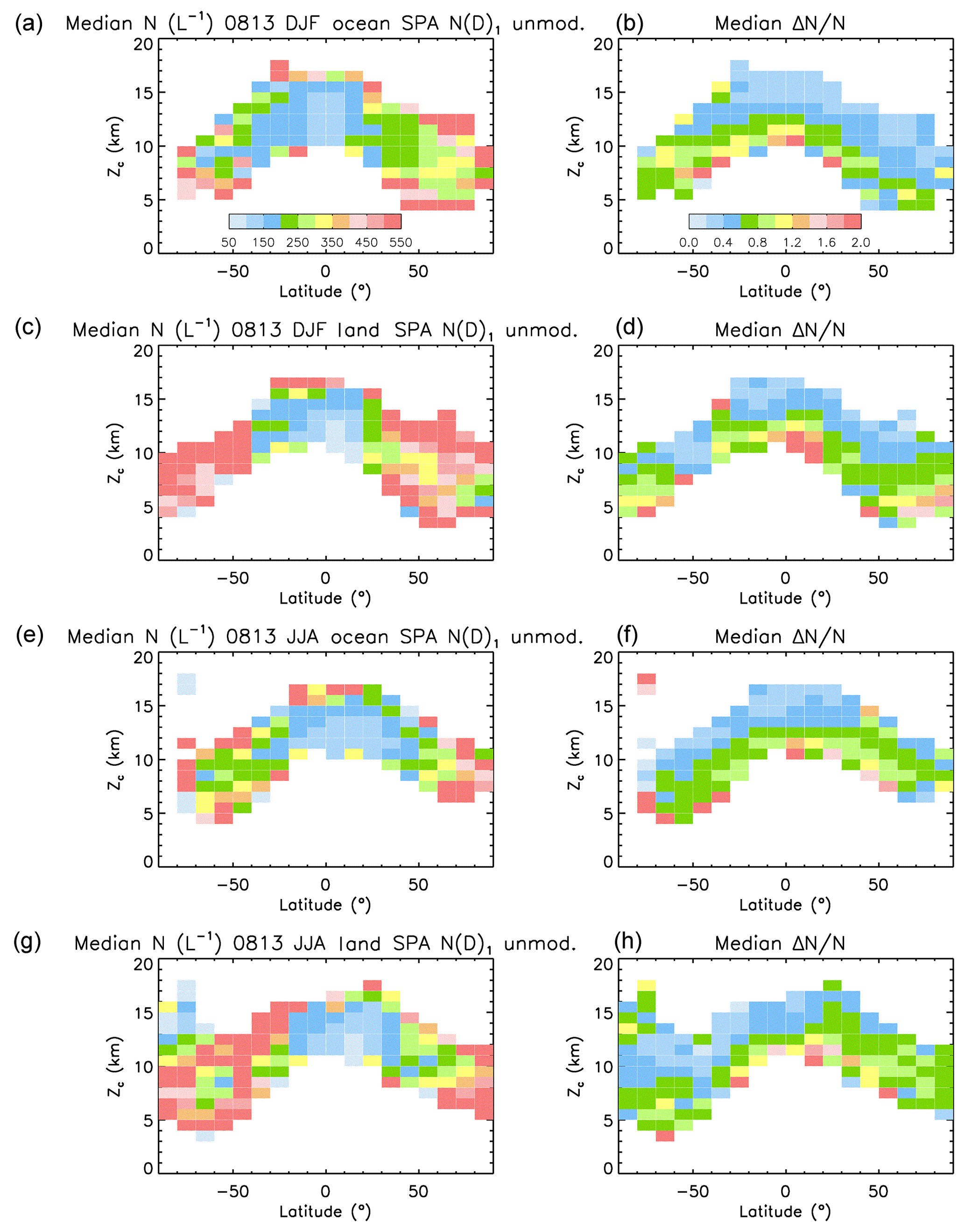
Figure 9Median ice-particle number concentration N (L−1) retrieved from the SPARTICUS relationships assuming N(D)1 unmodified (a, c, e, g) and associated relative uncertainty ΔN∕N (b, d, f, h) vs. latitude and representative cloud altitude, Zc, during 2008 and 2013. Panels from top to bottom are for DJF over oceans, DJF over land, JJA over oceans, and JJA over land.
Figure 9 shows the latitude and altitude dependence of median N (left) and median ΔN∕N based on the SPARTICUS data with N(D)1 unmodified relationships, and Fig. S9 shows median N based on the three other formulations, with SPARTICUS N(D)1=0, TC4 N(D)1 unmodified, and TC4 N(D)1=0 from left to right. The difference between the four formulations varies with βeff as shown in Fig. 5. As in Fig. 8, the panels from top to bottom are for DJF over oceans and land, and JJA over oceans and land. The number of samples can be seen in Fig. 8. Median ΔN∕N, which varies strongly with βeff (Fig. S4), is typically smaller than 60 % when βeff is larger, but often larger than 100 % at the lowest altitudes where βeff is smaller.
Median N is the lowest in the tropics (i.e., 20∘ S–20∘ N), and retrieved values depend on the assumptions used, but are generally smaller than about 200 particles per liter. Over Antarctica during winter (JJA), the samples exhibiting centroid altitudes between 10–11 and 18 km corresponding to PSCs have lower N than the cirrus just below them around 9–11 km.
Figure S10 in the Supplement shows the same results as in Fig. 9, but uses a relaxed threshold of OD > 0.1. Consistent with Fig. S5, median N is decreased, by a factor 1.5 on average, while ΔN∕N is more than doubled.
5.3 Dependence of N on distance below cloud top
Our retrievals are now examined against both Tc and Tc−Ttop to estimate the impact of the distance from cloud top. These N retrievals are shown in Fig. 10 using the SPARTICUS N(D)1 unmodified assumption in the tropics (0–30∘) and at mid- (30–60∘) and high (60–82∘) latitudes in the winter and summer seasons (using both hemispheres) by distinguishing retrievals over oceans and over land. The associated number of samples is given in Fig. S11. Added to these figures are isolines of temperature differences between cloud base and cloud top (Tbase−Ttop). For most of the layers, Tc−Ttop represents 30 % to 70 % of Tbase−Ttop (Fig. S11). Figure 10 shows a strong dependence of N on Tc−Ttop, with high N (>500 L−1) seen near the top of the geometrically thin clouds ( ∘C), when Tc−Ttop is smaller than about 5 ∘C. In contrast, the N dependence on Tc is very weak (consistent with Fig. 7a, b, c). As seen in Figs. 10 and S11, the Tc−Ttop (and Tbase−Ttop) difference tends to be larger in the tropics than at mid- and high latitudes. The strong dependence of N on Tc−Ttop (Fig. 10) appears weakest at high latitudes and at mid-latitudes during winter over land, with N being relatively high there.
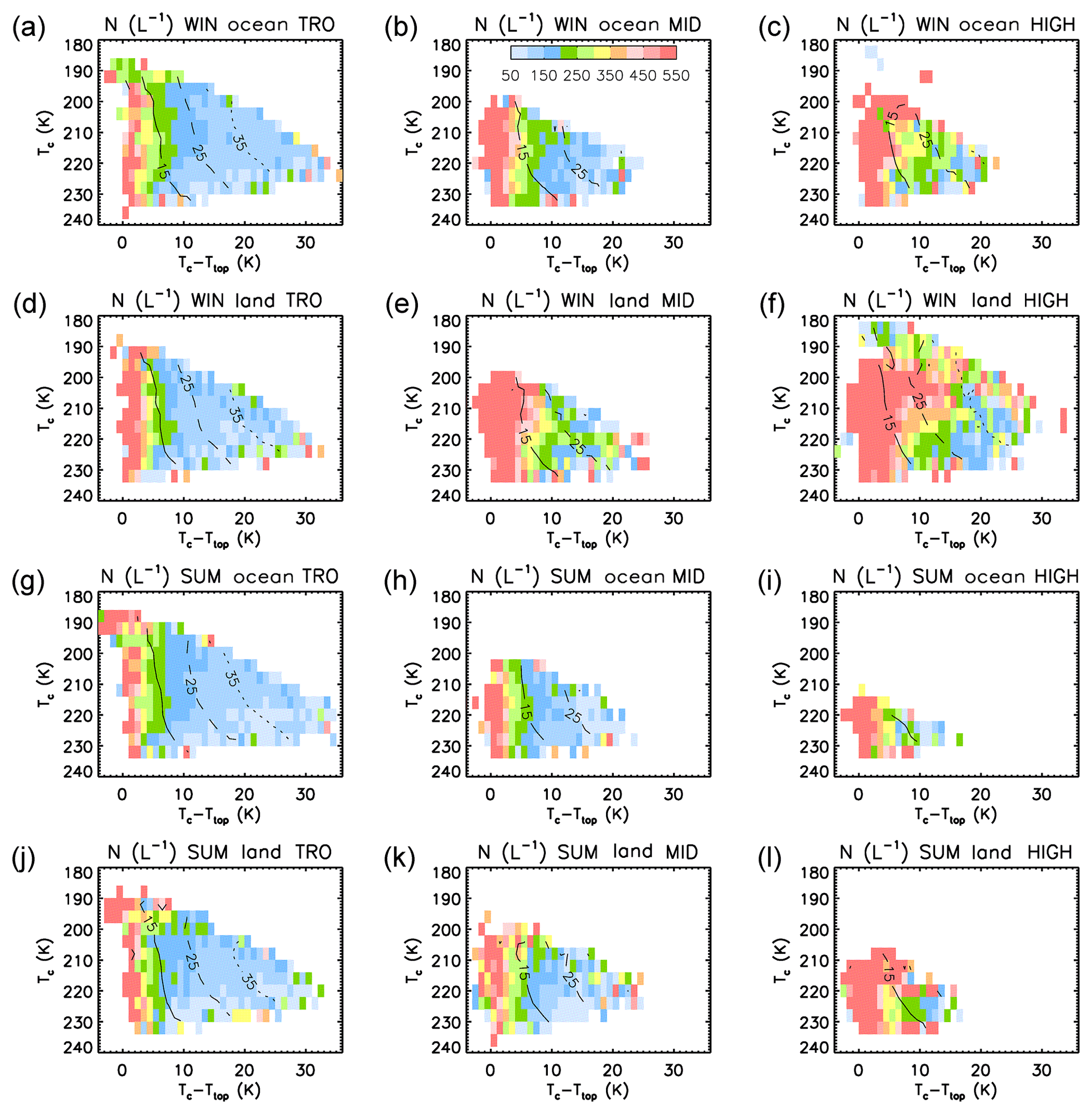
Figure 10Median retrieved ice-particle number concentrations N (L−1) using the SPARTICUS N(D)1 unmodified formulation related to the representative cloud temperature Tc and Tc−Ttop at 0–30∘ (TRO, a, d, g, j), 30–60∘ (MID, b, e, h, k) and 60–82∘ (HIGH, c, f, i, l) during 2008 and 2013. Overplotted are isolines of Tbase−Ttop (solid: 15 K, dashed: 25 K; dotted: 35 K). Panels from top to bottom are for winter over oceans, winter over land, summer over oceans and summer over land. TRO, MID and HIGH refer to the tropics, mid- and high latitudes.
5.4 Effective diameter
The dependence of median De on the representative temperature Tc is shown in Fig. 11 for each latitude zone (tropics, mid- and high latitudes), with profiles for summer and winter for each zone (based on both hemispheres), over oceans and land. The analysis is using the SPARTICUS unmodified N(D)1 (top) and the TC4 N(D)1=0 (bottom) formulations. The TC4 curve fits yield a larger range of De values than the SPARTICUS ones. At least 100 samples contributed to each data-point, and data from both years (2008 and 2013) were combined to generate these profiles. Consistent with the reported βeff–altitude relationships (Fig. 8), the De–temperature relationships show that De for a given temperature and season is generally largest in the tropics, intermediate at mid-latitudes and smallest in the high latitudes. The profiles exhibit a considerable latitudinal and seasonal dependence, with latitudinal differences up to ∼40 µm for a given temperature. Seasonal differences may be up to about 20 µm for a given temperature at mid-latitude over land. Combined with the latitudinal and seasonal dependence of selected cirrus cloud frequency of occurrence (e.g., Table 4), these De differences are likely to produce substantial variations in cirrus cloud net radiative forcing relative to a constant De profile assumption.
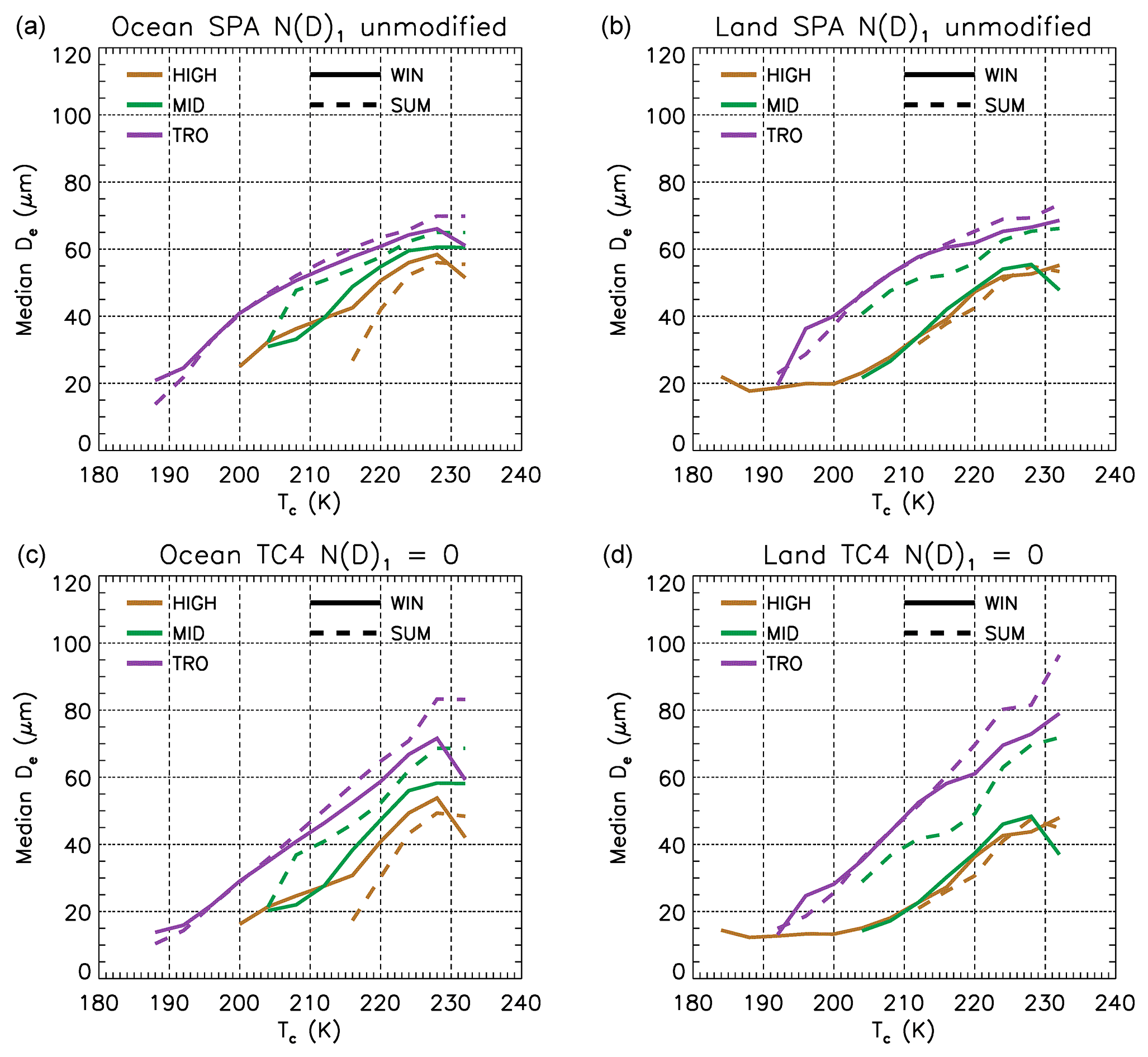
Figure 11Temperature dependence of the retrieved median effective diameter De (µm) in winter (solid) and summer (dashed) during 2008 and 2013, based on the SPARTICUS N(D)1 unmodified (a, b) and the TC4 N(D)1=0 (c, d) formulations. Latitude zones are denoted by colors: purple: 0–30∘ (TRO); green: 30–60∘ (MID); and brown: 60–82∘ (HIGH).
Following the same reasoning as previously used for N, Fig. S12 shows the dependence of median De (using the SPARTICUS N(D)1 unmodified assumption) on Tc and Tc−Ttop, for the same latitude ranges and seasons as in Figs. 10 and 11. Unlike N (Fig. 10), median De depends strongly on Tc with a somewhat weaker dependence on Tc−Ttop. For instance, in the tropics, small median De (<50 µm) are found at any Tc colder than about 205 K, but only near cloud top when Tc is warmer than 205 K. At Tc=220 K, median De increases with Tc−Ttop from less than 50 µm near cloud top up to the upper retrieval limit around 80 µm at K. This weaker dependence on Tc−Ttop relative to N is expected since De is proportional to IWC∕APSD. For a gamma function PSD and assuming power law relationships for ice-particle area and mass, De is proportional to λσ−β where λ=PSD slope parameter and σ and β are power law exponents for area and mass, respectively. The difference σ−β is slightly more than −1, showing that De is strongly related to the PSD mean size (inversely proportional to λ). The derivation also shows that De is not dependent on N. The decrease in De with decreasing Tc is likely due to a decrease in IWC with decreasing Tc.
6.1 Global and seasonal distribution of N
In the tropics, most cirrus are anvil cirrus and there is little difference in N between land and ocean, nor is there much seasonal dependence. A seasonal variation is seen in the NH at mid-latitude, more over land than over oceans, with larger N (and smaller De) during the winter than during the summer season (see Figs. 9 and S9). This behavior is less evident over land in the SH where mid-latitude land mass is relatively small, but over the Southern Ocean where ice nuclei (IN) concentrations are relatively low (Vergara-Temprado, 2018), N is larger (and De smaller) during winter. At high latitudes, N is relatively high and De relatively low during both seasons. These observations appear generally consistent with the modeling results of Storelvmo and Herger (2014), where the Community Atmosphere Model Version 5 (CAM5) was used to predict the global distribution of mineral dust at 200 hPa by season and the fraction of ice crystals produced by het and hom. Dust concentrations in both hemispheres were minimal at high latitudes, especially during DJF. If dust is the main source of IN (e.g., Cziczo et al., 2013) and more ice crystals are produced through hom when dust concentrations are relatively low (e.g., Haag et al., 2003), then the above observations appear consistent with the predicted latitude dependence of dust concentrations. That is, lower IN concentrations may result in higher RHi sufficient for hom to occur since the limited numbers of ice crystals produced via het may not exhibit sufficient surface area to draw down the RHi and prevent hom from occurring. While hom does not always result in relatively high N (e.g., Spichtinger and Krämer, 2013), hom can produce much higher N than het within sustained appreciable updrafts and is generally associated with higher N (e.g., Barahona and Nenes, 2008). Other observational studies indicating that hom is often important in determining the microphysics of cirrus clouds are Mitchell et al. (2016), Zhao et al. (2018), Sourdeval et al. (2018a) and Gryspeerdt et al. (2018).
Atmospheric dynamics may also help to explain the results in Fig. 9. The tropical troposphere is well mixed due to deep convection, whereas in the mid-latitudes during winter, deep mixing is more limited. This reduced mixing should reduce the transport of IN to cirrus cloud levels (relative to the tropics). Snow cover during winter may also limit dust transport. Indeed, N is considerably higher during winter over land in the NH mid-latitudes, and a similar but somewhat weaker seasonal relationship exists over oceans in the NH and SH mid-latitudes.
In general, we find higher N over mountainous regions, and mountain-induced waves may be responsible for higher N in the NH mid-latitudes, especially during the winter season (having higher winds). The Andes in South America provide abrupt orography for mountain-induced waves that provide high updrafts favoring hom (Jiang et al., 2002; Hoffmann et al., 2016). This abrupt orography combined with minimal mineral dust concentrations in this region, especially during DJF (Storelvmo and Herger, 2014), may explain the higher N over the Andes. However, N over the Andes was not higher in the tropics (Mitchell et al., 2016), perhaps due to higher IN concentrations in the tropics, lower sustained winds and the OD range sampled. Lower dust concentrations (Vergara-Temprado, 2018) may also be responsible for the higher N over the Southern Ocean.
6.2 Dependence of N on distance from cloud top
The temperature dependence of N on the cloud representative temperature Tc, as shown in Fig. 7a, b, c, is an important relationship for understanding the physics of cirrus clouds. However, the in-cloud dependence of N on height below cloud top may also be important. The strong N dependence on Tc−Ttop shown in Fig. 10 appears to support the lower updraft cirrus cloud simulations of Spichtinger and Gierens (2009a,b) and the in situ measurements of Diao et al. (2015). It could be enhanced by the fact that Tc−Ttop is somewhat correlated with geometrical thickness. In geometrically thin cirrus, there is less dilution of the mean N due to ice sedimentation (Jensen et al., 2013a). Also, in geometrically thicker cirrus, sedimenting ice particles from above tend to quench hom in the mid-to-lower cloud by decreasing the RHi, preventing the threshold RHi needed for hom. This can decrease N considerably (Spichtinger and Geirens, 2009a,b). This effect would tend to produce higher N in geometrically thin cirrus relative to the thicker cirrus. Moreover, aggregation has less time to decrease N in thin cirrus.
6.3 Representativeness of these results
As mentioned, the cirrus clouds sampled in this study are optically thick () and contribute a relatively small fraction of total cirrus cloud coverage according to some cirrus cloud climatologies (e.g., Kienast-Sjögren et al., 2016; Goldfarb et al., 2001; Immler and Schrems, 2002). Thus, it is possible that the cirrus cloud properties retrieved here are not representative of cirrus clouds in general. However, these are ground-based lidar studies conducted at point locations whereas the global cirrus cloud climatology in Hong and Liu (2015) is based on the CALIPSO and CloudSat satellites. In that satellite study, where the ice cloud OD ranged from <0.03 to >20, the frequency of occurrence for cirrus that have is much larger than these ground-based climatologies indicate, and this OD category appears to have the highest frequency of occurrence (see Fig. 7 of Hong and Liu, 2015). Moreover, in Kienast-Sjögren et al. (2016) where cirrus that have OD>0.3 comprised a very small fraction of the cirrus sampled, cirrus that have OD>0.3 still accounted for about half of the cloud net radiative forcing for cirrus cloud overcast conditions. If the Hong and Liu study is more realistic, then cirrus that have should strongly dominate the overall cirrus cloud net radiative forcing.
6.4 Comparisons with other studies
Figure 12 shows the geographical distribution of median N based on the years 2008 and 2013, with N retrieved using the SPARTICUS unmodified (left) and TC4 N(D)1=0 formulations (right), which correspond to the upper and lower N bounds, respectively. Figure 12 is for layers of representative temperature, Tc, between 218 and 228 K. When averaging over all temperature levels sampled (not shown), our results are still similar to those reported in Fig. 12. The geographical distributions of the number of samples and of median Tc−Ttop corresponding to Fig. 12 are shown in Fig. S13 in the Supplement. Median Tc−Ttop is up to 20 ∘C and is smaller at mid- to high latitudes than in the tropics. While the color legend in Fig. 12 changes color in increments of 50 L−1, the first color bin is from zero to 100 L−1 and the last color bin is from 500 L−1 to infinity. When comparing the two plots, regions corresponding to the highest N values may not change much due to this legend convention.
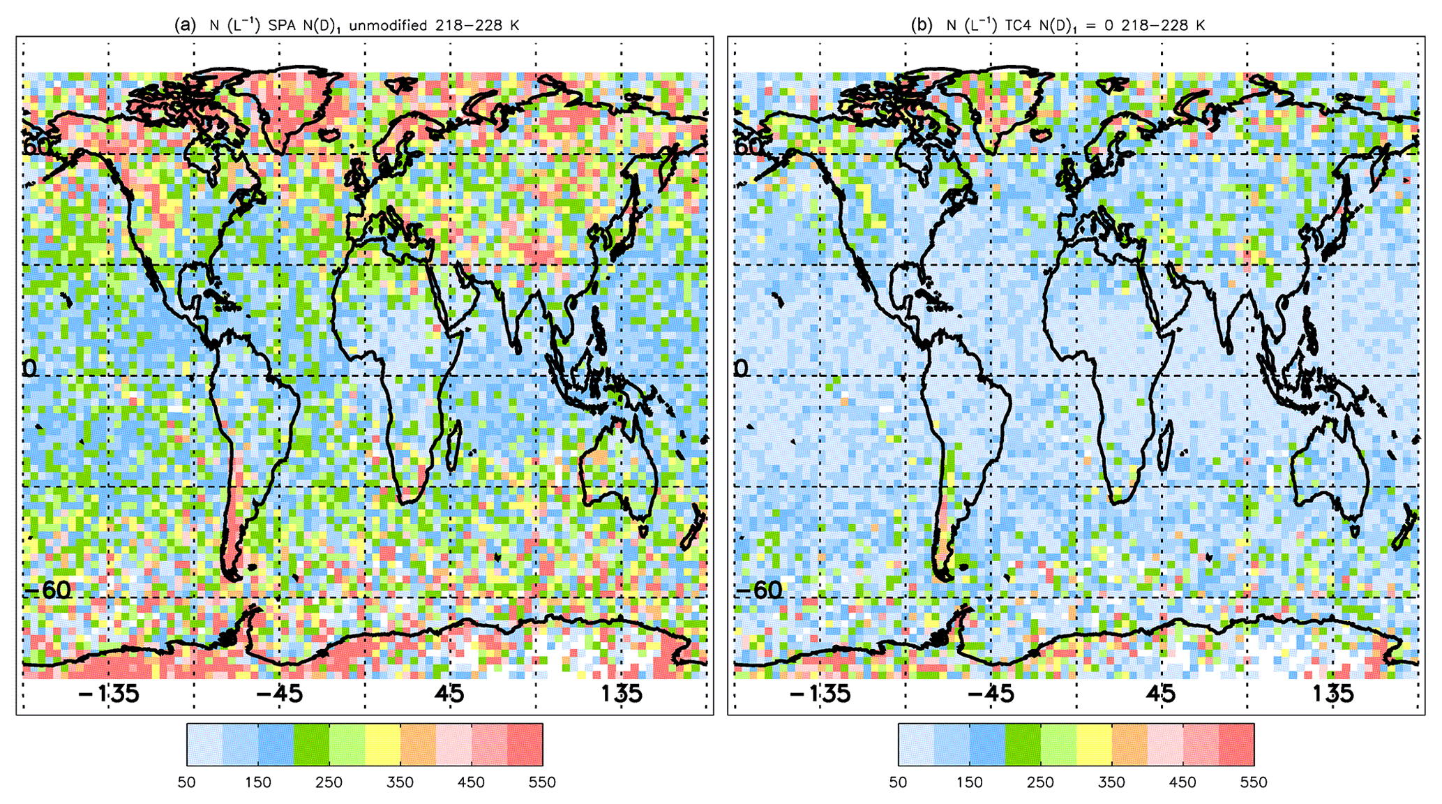
Figure 12Geographical distribution of median ice-particle number concentration N (L−1) during 2008 and 2013, where the layer representative temperature, Tc, is between 218 and 228 K. The retrievals use the following two formulations: SPARTICUS N(D)1 unmodified (a) and TC4 N(D)1=0 (b).
Results in Fig. 12 can be compared with the retrieved N values near cloud top at 223 K shown in Fig. 1 of Gryspeerdt et al. (2018). The geographical distributions are qualitatively similar, including higher N over mountainous regions and over the southern oceans, with minimal N over the tropics. Sourdeval et al. (2018a) have developed a new satellite retrieval for N regarding ice clouds, based on the CloudSat radar and the CALIPSO lidar (built upon the so-called DARDAR retrieval and referred to as the DARDAR-LIM scheme; LIM standing for Leipzig Institute for Meteorology). This retrieval uses the operational DARDAR retrieval products of IWC and (a PSD normalization factor that is a function of the IWC and Dm, where Dm is the ice-particle mean volume diameter, defined as the PSD moment ratio M4∕M3), and also the “universal” normalized PSD described in Delanoë et al. (2005), to estimate N. Although their retrieval scheme is based on different physics than our scheme, these schemes yield similar results. However, there are important differences. Since our scheme is based on in situ cirrus cloud PSDs, especially the smallest ice crystal sizes, it naturally suffers from uncertainties endemic to the PSD probes and uncertainties in how PSD shape may vary between regions (i.e., field campaigns). When βeff is greater than about 1.06, N retrievals vary by about a factor of 2 (Fig. 5), but N uncertainties are greater at smaller βeff where N∕IWC and De lose sensitivity to βeff. This limits our ability to retrieve at relatively low N. On the other hand, the DARDAR-LIM scheme estimates N using the normalized universal PSD described in Delanoë et al. (2005). This normalized PSD has the form , where N0 and k are constrained by the radar and lidar measurements, α and β are fixed constants, and Deq is the melted equivalent diameter of an ice particle. Whereas βeff determines the PSD fraction of small (D<50 µm) ice crystals in our scheme, this fraction is determined by α and k in the DARDAR-LIM scheme. Moreover, α depends on environmental conditions (Herzegh and Hobbs, 1985), with lower α values (which promote higher N) associated with higher updrafts and ice crystal production rates (such as might be found in cirrus clouds over mountainous terrain). Furthermore, radar measurements are not sensitive to small particles (Deng et al., 2010, 2013), in contrast to the lidar and to the IIR, and DARDAR-LIM retrievals using the lidar-only mode rely strongly on a priori relationships to retrieve N. In a general sense, in the case of clouds detected only by the radar or only by the lidar, the DARDAR algorithm does not benefit from the synergism between these two measurements, making the a priori relationships essential to obtain closure.
The highest N values reported in Sourdeval et al. (2018a) and Gryspeerdt et al. (2018) are for ice particles larger than 5 µm. These values would be higher by a factor of about 1.7 if all ice particles larger than 1 µm were considered (Sourdeval et al., 2018b). This is important to note since the CALIPSO IIR retrieval has no cut-off size, and it is very sensitive to ice crystals in the 1 to 5 µm range (Fig. 1). Keeping this in mind, the CALIPSO N retrievals are comparable in value to the DARDAR-LIM N retrievals.
The regional variation in median N might be greater than indicated by Fig. 12. Regarding TC4 and Fig. 6b, the N(D)1=0 assumption yielded the best agreement between in situ and retrieved βeff, whereas a similar comparison with SPARTICUS data (Fig. 6a) may arguably favor the unmodified N(D)1 assumption (since PSD sampled at ∘C were from a single cirrus event). Thus it is possible that the TC4 N(D)1=0 formulation of our retrieval scheme is most representative for tropical cirrus and that the SPARTICUS N(D)1 unmodified version is most appropriate for mid-to-high latitudes. This would double the N range estimated from the color-bar legend in Fig. 12, with N varying by a factor of about 14 (note that N≪50 L−1 is within the dynamic retrieval range of the TC4 N(D)1=0 scheme, which is evident from Fig. 5 and Eq. 8).
Ice cloud CALIPSO-CloudSat retrievals of De are reported in Fig. 12 of Hong and Liu (2015) against temperature in terms of season and latitude zone for ODs ranging from <0.03 to >20. Keeping in mind the different cloud sampling (in particular OD range and our cloud base temperature being colder than 235 K), comparing their seasonal De changes with those in this study is not straight-forward. Nevertheless, mean De values are comparable, in particular for the TC4 N(D)1=0 assumption at temperatures colder than 235 K (the upper limit in this study). Their De in the tropics at 190 K is about 40 µm compared to 20 µm in this study. At 220 K, their De around 70 µm is in fair agreement with our De found between 60 and 70 µm. Heymsfield et al. (2014, their Fig. 11) report small De around 20 µm at temperature colder than −72 ∘C, in agreement with this study, but they find a steeper increase of De with temperature. Detailed comparisons with other work, which are beyond the scope of this paper, should account not only for temperature, but also for distance from cloud top.
6.5 A possible link between high latitude cirrus and mid-latitude weather
The retrieval results in Table 4 indicate that at high latitudes there tends to be the greatest cirrus cloud coverage during winter in the Arctic and during spring (SON) in the Antarctic (where relatively high N and small De occur throughout the year in both regions, as shown in Figs. 9, 11 and 12). While this study only considers a subset of cirrus clouds and 2 years of retrievals, our findings on the seasonal dependence of cirrus cloud coverage are consistent with other satellite cirrus cloud studies that consider a broader range of conditions over longer periods (Nazaryan et al., 2008; Hong and Liu, 2015). Independent of the macro- and microphysical cirrus cloud attributes found in this study, at high latitudes when the sun is near or below the horizon, cirrus clouds produce a strong net warming at the top of atmosphere (TOA) and at the surface (Hong and Liu, 2015; Storelvmo et al., 2014). This indicates that the strongest net radiative forcing by cirrus clouds on Arctic (Antarctic) climate occurs during winter (spring). Combined with the unique macro- and microphysical properties of Arctic cirrus during winter reported here, this suggests that wintertime Arctic cirrus may have a significant warming effect on Arctic climate. A satellite remote sensing study of ice clouds (T<0 ∘C) by Hong and Liu (2015) found that at high latitudes, ice cloud net radiative forcing at the TOA and at the surface during the cold season is >2 W m−2 for a cirrus cloud OD of 1.5. Since the most severe effects of global warming occur at high latitudes, it is critical to understand the factors controlling the macro- and microphysical properties of high latitude cirrus clouds.
A potential link to mid-latitude winter weather is the possible impact of the winter Arctic cirrus on the meridional (north–south) temperature gradient between the Arctic and mid-latitudes. The cirrus-induced winter warming described above will occur throughout the troposphere (Chen et al., 2000; Hong and Liu, 2015), and will thus act to reduce this temperature gradient in the upper troposphere (UT). While it is not clear how this would impact weather, some type of impact is likely if the warming is significant, and several possible scenarios are described in Cohen et al. (2014) and Barnes and Screen (2015). While many papers have been published recently regarding potential effects of Arctic Amplification (henceforth AA; the observation that the mean Arctic temperature rise due to greenhouse gases is at least a factor of two greater relative to the adjacent mid-latitudes) on mid-latitude weather, it is important to note that the AA related to sea ice loss and associated increases in sea surface temperature primarily affects temperatures between the surface and 700 hPa (Screen et al., 2012), while heating due to winter cirrus would strongly affect the UT. A theoretical link between AA and the jet-stream is found in the thermal wind balance, which states that a reduced meridional temperature gradient tends to produce a reduced vertical gradient in the zonal-wind field, depending on other factors like changes in surface winds, storm tracks and the tropopause height (Barnes and Screen, 2015). Thus, AA could lead to a weaker jet-stream having more amplified Rossby waves and associated extreme weather events as hypothesized by Francis and Vavrus (2012, 2015), but it is currently not clear whether such a phenomenon is occurring or will be occurring (Barnes and Screen, 2015).
As described in Barnes and Screen (2015), GCM simulations from the fifth Coupled Model Intercomparison Project (CMIP5) show that while the lower troposphere during Arctic winter is projected to warm substantially by 2100, this is not happening in the Arctic UT where little warming is projected. Moreover, in the tropics the models predict the strongest warming in 2100 will occur in the UT. These effects decrease the meridional temperature gradient at low levels and increase the temperature gradient in the UT. These low- and high-level gradients have competing effects on the jet-stream, with a decreasing low-level gradient acting to weaken the jet-stream and shift it towards the equator, while an increasing UT gradient acts to strengthen the jet-stream and shift it poleward (Barnes and Screen, 2015). An interesting question to ask here is whether the CMIP5 GCMs adequately describe the changes in winter Arctic cirrus that satellite remote sensing studies observe. If they do not, and the winter heating from Arctic cirrus clouds is underestimated in the models, then the meridional UT temperature gradient may be overestimated during winter. Future GCM research should strive for consistency with Arctic cloud observations from satellites to determine whether the UT heating from the winter Arctic cirrus could be a significant factor affecting the simulated NH mid-latitude circulation.
A related question is whether wintertime Arctic cirrus are increasing, causing a change in jet-stream behavior. Poleward transport of heat and moisture is a fundamental attribute of the Earth's climate system, and the atmosphere of a warming climate can hold more water vapor (Dufour et al., 2016). While mid-latitude frontal systems are a primary component of this poleward transport, extreme transport events that can be described as water vapor intrusions (WVI) may account for 28 % of the total moisture transport into the Arctic (Woods et al., 2013). During WVIs, low-level winds from below the Arctic Circle (66∘ N) penetrate deep into the Arctic mostly during winter (Johansson et al., 2017). These WVIs destabilize the Arctic boundary layer, and can increase both low- and high-cloud coverage over the Arctic, with cirrus clouds increasing mostly in winter by 15 %–30 %. Both Screen et al. (2012) and Francis and Vavrus (2015) found evidence of increased remote energy transport into the Arctic, especially after 2000. This occurred mostly during the fall through enhanced planetary wave amplitudes (Francis and Vavrus, 2015). This transport may have contributed to the observed increase of Arctic cirrus clouds during winter (Table 4). These remote effects may enhance Arctic winter cirrus and their associated heating rates, which may affect jet-stream dynamics.
A new satellite remote sensing method was developed to retrieve the ice-particle number concentration N within cirrus clouds, along with effective diameter De, extinction coefficient and ice water content (IWC). This was made possible by exploiting the fact that most of the difference in retrieved absorption optical depth (τabs) in the split-window channels at 12.05 and 10.6 µm is due to wave resonance absorption, a process sensitive to the smallest ice crystals that dominate N (Mitchell et al., 2010). Due to this process, a tight relationship between N∕IWC and βeff [τabs(12 µm)∕τabs(10.6 µm)] was obtained using PSD aircraft measurements. This relationship, and a similar tight relationship between De and βeff, are the unique aspects of this retrieval and make it self-consistent through the shared dependence on βeff. Perhaps the most unique aspect of this retrieval method is its sensitivity to small ice crystals via βeff. The sensitivity ranges ( g−1 & De<90–110 µm) are usually compatible with cirrus clouds ( ∘C) since PSDs tend to be narrower at these temperatures, containing relatively small ice particles.
The N retrieval uses βeff derived from IIR–CALIOP measurements. Although the retrieval is restricted to single-layer cirrus cloud ODs between about 0.3 and 3.0 (which excludes most TTL cirrus), this OD range is likely to be the most radiatively significant range due to the lower cirrus cloud frequency of occurrence at ODs > 3 and a much lower cirrus cloud mean emissivity at ODs < 0.3 (Hong and Liu, 2015). In other words, for the sampled single layer clouds, the cirrus clouds that the IIR senses best in the window channels will also have the most influence on the Earth's longwave radiation budget. Four formulations of the retrieval were used, based on either the SPARTICUS or TC4 field campaigns, with the smallest size bin of the 2D-S probe either assumed as valid (N(D)1 unmodified) or by assuming N(D)1=0. The SPARTICUS unmodified N(D)1 assumption gives the highest N values while the TC4 N(D)1=0 assumption yielded the lowest N values. The N predicted from these two formulations differed by a factor of two (see Fig. 5), thus defining a possible systematic uncertainty in N. The random relative uncertainty, ΔN∕N, is most of the time <0.5 for small crystals (De<35–50 µm), but increases up to more than 2 at the sensitivity limit.
A 2-year global and seasonal analysis of these CALIPSO observations reveals that N depends on the latitude zone, season and surface type (land vs. ocean). In the relatively pristine high latitudes, N was relatively high and De was relatively low, suggesting that homogeneous ice nucleation may be an important process at these latitudes. In the tropics, N was lowest and De was largest on average, relative to the high- and mid-latitudes, with little seasonal dependence. There was considerable seasonal dependence regarding median N and De in the mid-latitudes, with N being higher and De being smaller during winter (for a given temperature), especially over land in the NH and over ocean in the SH.
The objective of this paper was not to determine absolute magnitudes for the retrieved quantities, but rather to show how they vary in terms of temperature, cloud thickness, latitude, season and topography using any of the four formulations of this retrieval. For a given formulation, these relative differences were similar and were not sensitive to the retrieval formulation used. When the sample selection criteria were relaxed to accept samples that have cloud OD > 0.1 (instead of OD > 0.3), median N was reduced by a factor of 1.5 on average while ΔN∕N was more than doubled.
The N retrieval described herein is an advancement of the work described in Mitchell et al. (2016), which supports many of the findings in Gryspeerdt et al. (2018), including the dependence of homogeneous ice nucleation in cirrus clouds on topography and latitude. Consistent with other satellite studies on ice clouds, the optically thicker cirrus clouds we studied exhibited a seasonal dependence in the Arctic in regards to frequency of occurrence, with cirrus during winter at least twice as likely to occur relative to other seasons. This might have a significant effect on jet stream dynamics.
Future cirrus cloud field campaigns designed to sample small ice crystals in regions not representative of the TC4 and SPARTICUS domains (such as at high latitudes or over mid-latitude oceans) may further improve upon this retrieval framework. It may also be beneficial if more information relevant to remote sensing synergism is taken during in situ observations.
The following CALIPSO data products were used in this study: the V3.01 CALIPSO IIR level 2 track product (Vaughan et al., 2017; NASA Langley Research Center Atmospheric Science Data Center; https://doi.org/10.5067/IIR/CALIPSO/L2_Track-Beta-V3-01); the V3.30 CALIPSO IIR level 2 track product (Vaughan et al., 2017; NASA Langley Research Center Atmospheric Science Data Center; https://doi.org/10.5067/IIR/CALIPSO/L2_Track-Beta-V3-30); the V2.00 CALIPSO IIR level 1 product (Vaughan et al., 2017; NASA Langley Research Center Atmospheric Science Data Center; https://doi.org/10.5067/IIR/CALIPSO/Standard_L1B-V2-00); the V3.01 CALIPSO CALIOP 1/3 km cloud layer product (Vaughan et al., 2017; NASA Langley Research Center Atmospheric Science Data Center; https://doi.org/10.5067/CALIOP/CALIPSO/CAL_LID_L2_333mCLay-ValStage1-V3-01_L2-003.01); the V3.30 CALIPSO CALIOP 1/3 km cloud layer product (Vaughan et al., 2017; NASA Langley Research Center Atmospheric Science Data Center, https://doi.org/10.5067/CALIOP/CALIPSO/CAL_LID_L2_333mCLay-ValStage1-V3-30_L2-003.30); the V3.01 CALIPSO CALIOP 5 km cloud layer product (Vaughan et al., 2017; NASA Langley Research Center Atmospheric Science Data Center; https://doi.org/10.5067/CALIOP/CALIPSO/CAL_LID_L2_05kmCLay-Prov-V3-01_L2-003.01); the V3.30 CALIPSO CALIOP 5 km cloud layer product (Vaughan et al., 2017; NASA Langley Research Center Atmospheric Science Data Center; https://doi.org/10.5067/CALIOP/CALIPSO/CAL_LID_L2_05kmCLay-Prov-V3-30_L2-003.30); the V3.01 CALIPSO CALIOP 5 km cloud profile product (Vaughan et al., 2017; NASA Langley Research Center Atmospheric Science Data Center; https://doi.org/10.5067/CALIOP/CALIPSO/CAL_LID_L2_05kmCPro-Prov-V3-01_L2-003.01); the V3.30 CALIPSO CALIOP 5 km cloud profile product (Vaughan et al., 2017; NASA Langley Research Center Atmospheric Science Data Center; https://doi.org/10.5067/CALIOP/CALIPSO/CAL_LID_L2_05kmCPro-Prov-V3-30_L2-003.30). These data products are also available from the AERIS/ICARE Data and Services Center. Post-processed data are available upon request from the authors.
We begin this analysis with our retrieval equation for the ice-particle number concentration, N:
with g m−3. The quantities N∕IWC, De and (12 µm) are retrieved from βeff using the regression curves given in Table 1 for the four formulations. By writing x=βeff, they can be expressed as follows:
Equation (A1) can be re-written as follows:
with
and
Assuming a negligible error in ΔZeq, and writing τabs(12.05 µm) as τ12 and τabs(10.6 µm) as τ10 for more clarity, so that , the derivative of N can be written as follows:
In Eq. (A8), the derivative of x=βeff is
Errors in τ12 and in τ10 are computed by propagating errors in (i) the measured brightness temperatures Tm, (ii) the background brightness temperatures TBG and (iii) the blackbody brightness temperatures TBB (Garnier et al., 2015).
The uncertainties in Tm10 at 10.6 µm and in Tm12 at 12.05 µm are random errors set to 0.3 K according to the IIR performance assessment established by the Centre National d'Etudes Spatiales (CNES) assuming no systematic bias in the calibration. They are statistically independent.
Because the same cloud temperature is used to compute τ12 and τ10, the uncertainty ΔTBB is the same at 10.6 and at 12.05 µm. A random error of ±2 K is estimated to include errors in the atmospheric model.
After correcting for systematic biases based on differences between observations and computations (BTDoc) in cloud-free conditions, the random error ΔTBG in TBG is set from the standard deviation of the resulting distributions of BTDoc. As illustrated in Fig. S1a in the Supplement, nighttime and daytime standard deviations at 12.05 µm are similar over ocean, and found smaller than over land, where the deviations tend to be larger during daytime than at night. For simplicity, ΔTBG at 12.05 µm is set to ±1 K over ocean, and to ±3 K over land for both night and day. Standard distributions of BTDoc(10.6 µm)–BTDoc(12.05 µm) (Fig. S1b) indicate whether the errors in TBG at 10.6 and 12.05 µm are canceling out or not, after accounting for the contribution from the observations, which is estimated to K. Standard deviations of [BTDoc(10.6 µm)–BTDoc(12.05 µm)] are found smaller than 0.5 K over ocean and over land during nighttime, which indicates that the errors ΔTBG in TBG at 12.05 and at 10.6 µm can be considered identical. They are found locally up to 1 K during daytime over land, which could reflect a variability of the 10.6–12.05 difference in surface emissivity, but also the presence of residual clouds.
Finally, the relative uncertainty ΔN∕N is written as follows:
The supplement related to this article is available online at: https://doi.org/10.5194/acp-18-17325-2018-supplement.
DM and AG conceived the study; AG accessed and analyzed the CALIPSO data; DM accessed and analyzed the in situ data; JP provided expertise on the CALIPSO data and EE assisted with the in situ data analysis. All authors contributed to the writing of the paper.
The authors declare that they have no conflict of interest.
This research was supported primarily by NASA grant NNX16AM11G and the NASA
CALIPSO project. Earlier funding was provided by the Office of Science (BER),
US Department of Energy, and additional support was obtained through the CNES
Eeclat project. Melody Avery is deeply acknowledged for fruitful
discussions and her invaluable comments in the progress of this work.
Martina Krämer is gratefully acknowledged for providing us with the curve
fits that describe her 2009 data set of cirrus cloud in situ data. We are
also grateful to two referees who provided constructive feedback that has
improved this paper considerably. CALIPSO products are available at the
Atmospheric Science Data Center of the NASA Langley Research Center and at
the AERIS/ICARE Data and Services Center in Lille (France).
Edited by: Timothy Garrett
Reviewed by: two anonymous referees
Ackerman, S. A., Smith, W. L., Collard, A. D., Ma, X. L., Revercomb, H. E., and Knuteson, R. O.: Cirrus cloud properties derived from high spectral resolution infrared spectrometry during FIRE II, Part II: Aircraft HIS results, J. Atmos. Sci., 52, 4246–4263, 1995.
Baker, B. A. and Lawson, R. P.: Improvement in determination of ice water content from two-dimensional particle imagery, Part I: Image-to-mass relationships, J. Appl. Meteorol. Climatol., 45, 1282–1290, 2006a.
Baker, B. A. and Lawson, R. P.: In Situ Observations of the Microphysical Properties of Wave, Cirrus, and Anvil Clouds, Part I: Wave Clouds, J. Atmos. Sci., 63, 3160–3185, 2006b.
Barahona, D. and Nenes, A.: Parameterization of cirrus cloud formation in large-scale models: Homogeneous nucleation, J. Geophys. Res., 113, D11211, https://doi.org/10.1029/2007JD009355, 2008.
Barnes, E. A. and Screen, J. A.: The impact of Arctic warming on the midlatitude jet-stream: Can it? Has it? Will it? WIREs, Clim. Change, 6, 277–286, https://doi.org/10.1002/wcc.337, 2015.
Chen, T., Rossow, W., and Zhang, Y.: Radiative effects of cloud-type variations, J. Climate, 13, 264–286, 2000.
Cohen, J., Screen, J. A., Furtado, J. C., Barlow, M., Whittleston, D., Coumou, D., Francis, J., Dethloff, K., Entekhabi, D., Overland, J., and Jones, J.: Recent Arctic amplification and extreme mid-latitude weather, Nat. Geosci., 7, 627–637, 2014.
Cooper, S. J., L'Ecuyer, T. S., and Stephens, G. L.: The impact of explicit cloud boundary information on ice cloud microphysical property retrievals from infrared radiances, J. Geophys. Res., 108, 4107, https://doi.org/10.1029/2002JD002611, 2003.
Cooper, S. J. and Garrett, T. J.: Identification of Small Ice Cloud Particles Using Passive Radiometric Observations, J. Appl. Meteorol. Climatol., 49, 2334–2347, https://doi.org/10.1175/2010JAMC2466.1, 2010.
Cotton, R. J., Field, P. R., Ulanowski, Z., Kaye, P. H., Hirst, E., Greenaway, R. S., Crawford, I., Crosier, J., and Dorsey, J.: The effective density of small ice particles obtained from in situ aircraft observations of mid-latitude cirrus, Q. J. Roy. Meteorol. Soc., 139, 1923–1934, https://doi.org/10.1002/qj.2058, 2013.
Cziczo, D. J., Froyd, K. D., Hoose, C., Jensen, E. J., Diao, M., Zondlo, M.A., Smith, J. B., Twohy, C. H., and Murphy, D. M.: Clarifying the dominant sources and mechanisms of cirrus cloud formation, Science, 340, 1320–1324, https://doi.org/10.1126/science.1234145, 2013.
Delanoë, J. and Hogan, R. J.: A variational scheme for retrieving ice cloud properties from combined radar, lidar, and infrared radiometer, J. Geophys. Res., 113, D07204, https://doi.org/10.1029/2007JD009000, 2008.
Delanoë, J. and Hogan, R. J.: Combined CloudSat-CALIPSO-MODIS retrievals of the properties of ice clouds, J. Geophys. Res.-Atmos., 115, D00H29, https://doi.org/10.1029/2009JD012346, 2010.
Delanoë, J., Protat, A., Testud, J., Bouniol, D., Heymsfield, A. J., Bansemer, A., Brown, P. R. A., and Forbes, R. M.: Statistical properties of the normalized ice particle size distribution, J. Geophys. Res., 110, D10201, https://doi.org/10.1029/2004JD005405, 2005.
Deng, M., Mace, G. G., Wang, Z., and Okamoto, H.: Tropical Composition, Cloud and Climate Coupling Experiment validation for cirrus cloud profiling retrieval using CloudSat radar and CALIPSO lidar, J. Geophys. Res., 115, D00J15, https://doi.org/10.1029/2009JD013104, 2010.
Deng, M., Mace, G., Wang, Z., and Lawson, R. P.: Evaluation of Several A-Train Ice Cloud Retrieval Products with In Situ Measurements Collected during the SPartICus Campaign, J. Appl. Meteorol. Climatol., 52, 1014–1030, https://doi.org/10.1175/JAMC-D-12-054.1, 2013.
Diao, M., Jensen, J. B., Pan, L. L., Homeyer, C. R., Honomichl, S., Bresch, J. F., and Bansemer, A.: Distributions of ice supersaturation and ice crystals from airborne observations in relation to upper tropospheric dynamical boundaries, J. Geophys. Res.-Atmos., 120, 5101–5121, https://doi.org/10.1002/2015JD023139, 2015.
de Reus, M., Borrmann, S., Bansemer, A., Heymsfield, A. J., Weigel, R., Schiller, C., Mitev, V., Frey, W., Kunkel, D., Kürten, A., Curtius, J., Sitnikov, N. M., Ulanovsky, A., and Ravegnani, F.: Evidence for ice particles in the tropical stratosphere from in-situ measurements, Atmos. Chem. Phys., 9, 6775–6792, https://doi.org/10.5194/acp-9-6775-2009, 2009.
Dubuisson, P., Giraud, V., Chomette, O., Chepfer, H., and Pelon, J.: Fast radiative transfer modeling for infrared imaging radiometry, J. Quant. Spectrosc. Ra., 95, 201–220, 2005.
Dubuisson, P., Giraud, V., Pelon, J., Cadet, B., and Yang, P.: Sensitivity of thermal infrared radiation at the top of the atmosphere and the surface to ice cloud microphysics, J. Appl. Meteorol. Climatol., 47, 2545–2560, 2008.
Dufour, A., Zolina, O., and Gulev, S. K.: Atmospheric moisture transport to the Arctic: Assessment of reanalyses and analysis of transport components, J. Climate, 29, 5061–5081, https://doi.org/10.1175/JCLI-D-15-0559.1, 2016.
Eliasson, S., Buehler, S. A., Milz, M., Eriksson, P., and John, V. O.: Assessing observed and modelled spatial distributions of ice water path using satellite data, Atmos. Chem. Phys., 11, 375–391, https://doi.org/10.5194/acp-11-375-2011, 2011.
Erfani, E. and Mitchell, D. L.: Developing and bounding ice particle mass- and area-dimension expressions for use in atmospheric models and remote sensing, Atmos. Chem. Phys., 16, 4379–4400, https://doi.org/10.5194/acp-16-4379-2016, 2016.
Field, P. R., Heymsfield, A. J., and Bansemer, A.: Shattering and particle interarrival times measured by optical array probes in ice clouds, J. Atmos. Ocean. Technol., 23, 1357–1371, 2006.
Francis, J. A. and Vavrus, S. J.: Evidence linking Arctic amplification to extreme weather in mid-latitudes, Geophys. Res. Lett., 39, L06801, https://doi.org/10.1029/2012GL051000, 2012.
Francis, J. A. and Vavrus, S. J.: Evidence for a wavier jet stream in response to rapid Arctic warming, Environ. Res. Lett., 10, 014005, https://doi.org/10.1088/1748-9326/10/1/014005, 2015.
Fu, Q.: An accurate parameterization of the solar radiative properties of cirrus clouds for climate models, J. Climate, 9, 2058–2082, 1996.
Fu, Q.: A New Parameterization of an Asymmetry Factor of Cirrus Clouds for Climate Models, J. Atmos. Sci., 64, 4140–4150, 2007.
Garnier A., Pelon, J., Dubuisson, P., Faivre, M., Chomette, O., Pascal, N., and Kratz, D. P.: Retrieval of cloud properties using CALIPSO Imaging Infrared Radiometer, Part I: effective emissivity and optical depth, J. Appl. Meteorol. Climatol., 51, 1407–1425, https://doi.org/10.1175/JAMC-D-11-0220.1, 2012.
Garnier, A., Pelon, J., Dubuisson, P., Yang, P., Faivre, M., Chomette, O., Pascal, N., Lucker, P., and Murray, T.: Retrieval of cloud properties using CALIPSO Imaging Infrared Radiometer, Part II: effective diameter and ice water path, J. Appl. Meteor. Climatol., 52, 2582–2599, https://doi.org/10.1175/JAMC-D-12-0328.1, 2013.
Garnier, A., Pelon, J., Vaughan, M. A., Winker, D. M., Trepte, C. R., and Dubuisson, P.: Lidar multiple scattering factors inferred from CALIPSO lidar and IIR retrievals of semi-transparent cirrus cloud optical depths over oceans, Atmos. Meas. Tech., 8, 2759–2774, https://doi.org/10.5194/amt-8-2759-2015, 2015.
Garnier, A., Trémas, T., Pelon, J., Lee, K.-P., Nobileau, D., Gross-Colzy, L., Pascal, N., Ferrage, P., and Scott, N. A.: CALIPSO IIR Version 2 Level 1b calibrated radiances: analysis and reduction of residual biases in the Northern Hemisphere, Atmos. Meas. Tech., 11, 2485–2500, https://doi.org/10.5194/amt-11-2485-2018, 2018.
Goldfarb, L., Keckhut, P., Chanin, M.-L., and Hauchecorne, A.: Cirrus Climatological Results from Lidar Measurements at OHP (44∘ N, 6∘ E), Geophys. Res. Lett., 28, 1687–1690, 2001.
Gryspeerdt, E., Sourdeval, O., Quaas, J., Delanoë, J., Krämer, M., and Kühne, P.: Ice crystal number concentration estimates from lidar-radar satellite remote sensing – Part 2: Controls on the ice crystal number concentration, Atmos. Chem. Phys., 18, 14351–14370, https://doi.org/10.5194/acp-18-14351-2018, 2018.
Guimaraes, L. G. and Nussenzveig, H. M.: Theory of Mie resonances and the ripple fluctuations, Opt. Commun., 89, 363–369, 1992.
Gurganus, C. and Lawson, R. P.: Laboratory and Flight Tests of 2D Imaging Probes: Toward a Better Understanding of Instrument Performance and the Impact on Archived Data, J. Atmos. Ocean. Tech., 35, 1533–1553, https://doi.org/10.1175/JTECH-D-17-0202.1, 2018.
Haag, W., Kärcher, B., Ström, J., Minikin, A., Lohmann, U., Ovarlez, J., and Stohl, A.: Freezing thresholds and cirrus cloud formation mechanisms inferred from in situ measurements of relative humidity, Atmos. Chem. Phys., 3, 1791–1806, https://doi.org/10.5194/acp-3-1791-2003, 2003.
Heidinger, A. and Pavolonis, M. J.: Gazing at cirrus clouds for 25 years through a split window, Part I: Methodology, J. Appl. Meteorol. Climatol., 48, 1100–1116, 2009.
Herzegh, P. and Hobbs, P. V.: Size spectra of ice particles in frontal clouds: correlations between spectrum shape and cloud conditions, Q. J. Roy. Meteorol. Soc., 111, 463–477, 1985.
Heymsfield, A., Winker, D., Avery, M., Vaughan, M., Diskin, G., Deng, M., Mitev, V., and Matthey, R.: Relationships between ice water content and volume extinction coefficient from in situ observations for temperatures from 0∘ to −86 ∘C: Implications for spaceborne lidar retrievals, J. Appl. Meteorol. Climatol., 53, 479–505, https://doi.org/10.1175/JAMC-D-13-087.1, 2014.
Hoffmann, L., Grimsdell, A. W., and Alexander, M. J.: Stratospheric gravity waves at Southern Hemisphere orographic hotspots: 2003–2014 AIRS/Aqua observations, Atmos. Chem. Phys., 16, 9381–9397, https://doi.org/10.5194/acp-16-9381-2016, 2016.
Hong, Y. and Liu, G.: The characteristics of ice cloud properties derived from CloudSat and CALIPSO measurements, J. Climate, 28, 3880–3900, 2015.
Immler, F. and Schrems, O.: Determination of tropical cirrus properties by simultaneous LIDAR and radiosonde measurements, Geophys. Res. Lett., 29, 2090, https://doi.org/10.1029/2002GL015076, 2002.
Inoue, T.: On the temperature and emissivity determination of semitransparent cirrus clouds by bispectral measurements in the 10 µm window region, J. Meteorol. Soc. Jpn., 63, 88–98, 1985.
Jensen, E. J., Lawson, R. P., Bergman, J. W., Pfister, L., Bui, T. P., and Schmitt, C. G.: Physical processes controlling ice concentrations in synoptically forced, midlatitude cirrus, J. Geophys. Res.-Atmos., 118, 5348–5360, https://doi.org/10.1002/jgrd.50421, 2013a.
Jensen, E. J., Diskin, G., Lawson, R. P., Lance, S., Bui, T. P., Hlavkad, D., McGille, M., Pfister, L., Toon, O. B., and Gao, R.: Ice nucleation and dehydration in the Tropical Tropopause Layer, P. Natl. Acad. Sci. USA, 110, 2041–2046, https://doi.org/10.1073/pnas.1217104110, 2013b.
Jiang, J., Wu, D. L., and Eckermann, S. D.: Upper Atmospheric Research Satellite (UARS) MLS observation of mountain waves over the Andes, J. Geophys. Res., 107, 8273, https://doi.org/10.1029/2002JD002091, 2002.
Johansson, E., Devasthale, A., Tjernström, M., Ekman, A. M. L., and L'Ecuyer, T.: Response of the lower troposphere to moisture intrusions into the Arctic, Geophys. Res. Lett., 44, 2527–2536, https://doi.org/10.1002/2017GL072687, 2017.
Kienast-Sjögren, E., Rolf, C., Seifert, P., Krieger, U. K., Luo, B. P., Krämer, M., and Peter, T.: Climatological and radiative properties of midlatitude cirrus clouds derived by automatic evaluation of lidar measurements, Atmos. Chem. Phys., 16, 7605–7621, https://doi.org/10.5194/acp-16-7605-2016, 2016.
Korolev, A. V., Emery, E. F., Strapp, W., Cober, S. G., Isaac, G. A., Wasey, M., and Marcotte, D.: Small ice particles in tropospheric clouds: Fact or artifact?, B. Am. Meteor. Soc., August, 967–973, https://doi.org/10.1175/2010BAMS3141.1, 2011.
Krämer, M., Schiller, C., Afchine, A., Bauer, R., Gensch, I., Mangold, A., Schlicht, S., Spelten, N., Sitnikov, N., Borrmann, S., de Reus, M., and Spichtinger, P.: Ice supersaturations and cirrus cloud crystal numbers, Atmos. Chem. Phys., 9, 3505–3522, https://doi.org/10.5194/acp-9-3505-2009, 2009.
Lawson, R. P.: Effects of ice particles shattering on the 2D-S probe, Atmos. Meas. Tech., 4, 1361–1381, https://doi.org/10.5194/amt-4-1361-2011, 2011.
Lawson, R. P., O'Connor, D., Zmarzly, P., Weaver, K., Baker, B. A., Mo, Q., and Jonsson, H.: The 2D-S (Stereo) Probe: Design and preliminary tests of a new airborne, high speed, high-resolution particle imaging probe, J. Atmos. Ocean. Tech., 23, 1462–1477, 2006a.
Lawson, R. P., Baker, B., Pilson, B., and Mo, Q.: In situ observations of the microphysical properties of wave, cirrus, and anvil clouds, Part II: Cirrus clouds, J. Atmos. Sci., 63, 3186–3203, 2006b.
Lawson, R. P., Pilson, B., Baker, B., Mo, Q., Jensen, E., Pfister, L., and Bui, P.: Aircraft measurements of microphysical properties of subvisible cirrus in the tropical tropopause layer, Atmos. Chem. Phys., 8, 1609–1620, https://doi.org/10.5194/acp-8-1609-2008, 2008.
Lawson, R. P., Jensen, E., Mitchell, D. L., Baker, B., Mo, Q., and Pilson, B.: Microphysical and radiative properties of tropical clouds investigated in TC4 and NAMMA, J. Geophys. Res., 115, D00J08, https://doi.org/10.1029/2009JD013017, 2010.
Luebke, A. E., Afchine, A., Costa, A., Grooß, J.-U., Meyer, J., Rolf, C., Spelten, N., Avallone, L. M., Baumgardner, D., and Krämer, M.: The origin of midlatitude ice clouds and the resulting influence on their microphysical properties, Atmos. Chem. Phys., 16, 5793–5809, https://doi.org/10.5194/acp-16-5793-2016, 2016.
Mishra, S., Mitchell, D. L., and DeSlover, D.: Ground based retrievals of small ice crystals and water phase in Arctic cirrus, AIP Conference Proceedings 1100, Current Problems in Atmospheric Radiation (IRS 2008), in: Proceedings of the International Radiation Symposium (IRC/IAMAS), edited by: Nakajima, T. and Yamasoe, M. A., Foz de Iguassu, Brazil, 3–8 August 2008, 482–485, 2009.
Mishra, S., Mitchell, D. L., Turner, D. D., and Lawson, R. P.: Parameterization of ice fall speeds in midlatitude cirrus: results from SPartICus, J. Geophys. Res.-Atmos., 119, 3857–3876, https://doi.org/10.1002/2013jd020602, 2014.
Mitchell, D. L.: Parameterization of the Mie extinction and absorption coefficients for water clouds, J. Atmos. Sci., 57, 1311–1326, 2000.
Mitchell, D. L.: Effective diameter in radiation transfer: general definition, applications, and limitations, J. Atmos. Sci., 59, 2330–2346, https://doi.org/10.1175/1520-0469(2002)059<2330:edirtg>2.0.co;2, 2002.
Mitchell, D. L. and d'Entremont, R. P.: Satellite remote sensing of small ice crystal concentrations in cirrus clouds, AIP Conference Proceedings 1100, Current Problems in Atmospheric Radiation (IRS 2008), in: Proceedings of the International Radiation Symposium (IRC/IAMAS), edited by: Nakajima, T. and Yamasoe, M. A., Foz de Iguassu, Brazil, 3–8 August 2008, 185–188, 2009.
Mitchell, D. L. and d'Entremont, R. P.: Satellite retrieval of the liquid water fraction in tropical clouds between −20 and −38 ∘C, Atmos. Meas. Tech., 5, 1683–1698, https://doi.org/10.5194/amt-5-1683-2012, 2012.
Mitchell, D. L., Macke, A., and Yangang, L.: Modeling cirrus clouds, Part II: Treatment of radiative properties, J. Atmos. Sci., 53, 2967–2988, 1996a.
Mitchell, D. L., Chai, S. K., and Yangang, L.: Modeling cirrus clouds. Part I: Treatment of bimodal size spectra and case study analysis, J. Atmos. Sci., 53, 2952–2966, 1996b.
Mitchell, D. L., Arnott, W. P., Schmitt, C., Baran, A. J., Havemann, S., and Fu, Q.: Photon tunneling contributions to extinction for laboratory grown hexagonal columns, J. Q. Spectrosc. Ra., 70, 761–776, 2001.
Mitchell, D. L., Baran, A. J., Arnott, W. P., and Schmitt, C.: Testing and comparing the modified anomalous diffraction approximation, J. Atmos. Sci., 63, 2948–2962, https://doi.org/10.1175/jas3775.1, 2006.
Mitchell, D. L., d'Entremont, R. P., and Lawson, R. P.: Inferring cirrus size distributions through satellite remote sensing and microphysical databases, J. Atmos. Sci., 67, 1106–1125, https://doi.org/10.1175/2009jas3150.1, 2010.
Mitchell, D. L., Lawson, R. P., and Baker, B.: Understanding effective diameter and its application to terrestrial radiation in ice clouds, Atmos. Chem. Phys., 11, 3417–3429, https://doi.org/10.5194/acp-11-3417-2011, 2011a.
Mitchell, D. L., Mishra, S., and Lawson, R. P.: Representing the ice fall speed in climate models: results from tropical composition, cloud and climate coupling (TC4) and the indirect and semi-direct aerosol campaign (ISDAC), J. Geophys. Res.-Atmos., 116, D00t03, https://doi.org/10.1029/2010jd015433, 2011b.
Mitchell, D. L., Garnier, A., Avery, M., and Erfani, E.: CALIPSO observations of the dependence of homo- and heterogeneous ice nucleation in cirrus clouds on latitude, season and surface condition, Atmos. Chem. Phys. Discuss., https://doi.org/10.5194/acp-2016-1062, 2016.
Moosmüller, H., and Sorensen, C. M.: Single scattering albedo of homogeneous, spherical particles in the transition regime, J. Quant. Spectrosc. Ra., 219, 333–338, https://doi.org/10.1016/j.jqsrt.2018.08.015, 2018.
Muhlbauer, A., Ackerman, T. P., Comstock, J. M., Diskin, G. S., Evans, S. M., Lawson, R. P., and Marchand, R. T.: Impact of large-scale dynamics on the microphysical properties of midlatitude cirrus, J. Geophys. Res.-Atmos., 119, 3976–3996, https://doi.org/10.1002/2013JD020035, 2014.
Nazaryan, H., McCormick, M. P., and Menzel, W. P.: Global characterization of cirrus clouds using CALIPSO data, J. Geophys. Res., 113, D16211, https://doi.org/10.1029/2007JD009481, 2008.
Nussenzveig, H. M.: The theory of the rainbow, Sci. Amer., 236, 116–127, 1977.
Nussenzveig, H. M. and Wiscombe, W. J.: Diffraction as tunneling, Phys. Rev. Lett., 59, 1667–1670, 1987.
Nussenzveig, H. M.: Does the glory have a simple explanation? Optics Lett., 27, 1379–1381, 2002.
Parol, F., Buriez, J. C., Brogniez, G., and Fouquart, Y.: Information content of AVHRR channels 4 and 5 with respect to the effective radius of cirrus cloud particles, J. Appl. Meteorol., 30, 973–984, 1991.
Pavolonis, M. J.: Advances in extracting cloud composition information from spaceborne infrared radiances – A robust alternative to brightness temperatures, Part I: Theory, J. Appl. Meteorol. Climatol., 49, 1992–2012, 2010.
Schiller, C., Krämer, M., Afchine, A., Spelten, N., and Sitnikov, N.: The ice water content in Arctic, midlatitude and tropical cirrus, J. Geophys. Res., 113, D24208, https://doi.org/10.1029/2008JD010342, 2008.
Screen, J. A., Deser, C., and Simmonds, I.: Local and remote controls on observed Arctic warming, Geophys. Res. Lett., 39, L10709, https://doi.org/10.1029/2012GL051598, 2012.
Sourdeval, O., Labonnote, L. C., Baran, A. J., Mülmenstädt, J., and Brogniez, G.: A Methodology for Simultaneous Retrieval of Ice and Liquid Water Cloud Properties, Part II: Near-global Retrievals and Evaluation against A-Train Products, Q. J. Roy. Meteorol. Soc., 142, 3063–3081, https://doi.org/10.1002/qj.2889, 2016.
Sourdeval, O., Gryspeerdt, E., Krämer, M., Goren, T., Delanoë, J., Afchine, A., Hemmer, F., and Quaas, J.: Ice crystal number concentration estimates from lidar-radar satellite remote sensing, Part 1: Method and evaluation, Atmos. Chem. Phys., 18, 14327–14350, https://doi.org/10.5194/acp-18-14327-2018, 2018a.
Sourdeval, O.: Interactive comment on “Ice crystal number concentration estimates from lidar-radar satellite remote sensing. Part 1: Method and evaluation” by Odran Sourdeval et al., Atmos. Chem. Phys. Discuss., available at: https://www.atmos-chem-phys-discuss.net/acp-2018-20/acp-2018-20-AC2-supplement.pdf, 2018b.
Spichtinger, P. and Gierens, K. M.: Modelling of cirrus clouds – Part 1a: Model description and validation, Atmos. Chem. Phys., 9, 685–706, https://doi.org/10.5194/acp-9-685-2009, 2009a.
Spichtinger, P. and Gierens, K. M.: Modelling of cirrus clouds – Part 1b: Structuring cirrus clouds by dynamics, Atmos. Chem. Phys., 9, 707–719, https://doi.org/10.5194/acp-9-707-2009, 2009b.
Spichtinger, P. and Krämer, M.: Tropical tropopause ice clouds: a dynamic approach to the mystery of low crystal numbers, Atmos. Chem. Phys., 13, 9801–9818, https://doi.org/10.5194/acp-13-9801-2013, 2013.
Storelvmo, T. and Herger, N.: Cirrus cloud susceptibility to the injection of ice nuclei in the upper troposphere, J. Geophys. Res.-Atmos., 119, 2375–2389, https://doi.org/10.1002/2013JD020816, 2014.
Storelvmo, T., Boos, W. R., and Herger, N.: Cirrus cloud seeding: a climate engineering mechanism with reduced side effects?, Phil. Trans. R. Soc. A, 372, 20140116, https://doi.org/10.1098/rsta.2014.0116, 2014.
Stubenrauch, C. J., Rossow, W. B., Kinne, S., Ackerman, S., Cesana, G., Chepfer, H., Di Girolamo, L., Getzewich, B., Guignard, A., Heidinger, A., Maddux, B. C., Menzel, W. P., Minnis, P., Pearl, C., Platnick, S., Poulsen, C., Riedi, J., Sun-Mack, S., Walther, A., Winker, D., Zeng, S., and Zhao, Z.: : Assessment of global cloud datasets from satellites: Project and database initiated by the GEWEX radiation panel, B. Am. Meteor. Soc., 94, 1031–1049, 2013.
Toon, O. B., Starr, D. O., Jensen, E. J., Newman, P. A., Platnick, S., Schoeberl, M. R., Wennberg, P. O., Wofsy, S. C., Kurylo, M. J., Maring, H., Jucks, K. W., Craig, M. S., Vasques, M. F., Pfister, L., Rosenlof, K. H., Selkirk, H. B., Colarco, P. R., Kawa, S. R., Mace, G. G., Minnis, P., and Pickering, K. E.: Planning, implementation, and first results of the Tropical Composition, Cloud and Climate Coupling Experiment (TC4), J. Geophys. Res., 115, D00J04, https://doi.org/10.1029/2009JD013073, 2010.
Vaughan, M., Pitts, M., Trepte, C., Winker, D., Detweiler, P., Garnier, A., Getzewitch, B., Hunt, W., Lambeth, J., Lee, K.-P., Lucker, P., Murray, T., Rodier, S., Trémas, T., Bazureau, A., and Pelon, J.: CALIPSO data management system data products catalog, document No. PC-SCI-503, Release 4.20, available at: http://www-calipso.larc.nasa.gov/products/CALIPSO_DPC_Rev4x20.pdf (last access: 9 October 2018), 2017.
Vergara-Temprado, J., Miltenberger, A. K., Furtado, K., Grosvenor, D. P., Shipway, B. J., Hill, A. A., Wilkinson, J. M., Field, P. R., Murray, B. J., and Carslaw, K. S.: Strong control of Southern Ocean cloud reflectivity by ice-nucleating particles, P. Natl. Acad. Sci. USA, 115, 2687–2692, 2018.
Woods, C., Caballero, R., and Svensson, G.: Large-scale circulation associated with moisture intrusions into the Arctic during winter, Geophys. Res. Lett., 40, 4717–4721, https://doi.org/10.1002/grl.50912, 2013.
Woods, S., Lawson, R. P., Jensen, E., Bui, P., Thornberry, T., Rollins, A., Pfister, L., and Avery, M.: Microphysical Properties of Tropical Tropopause Layer Cirrus, J. Geophys. Res., 123, 6053–6069, https://doi.org/10.1029/2017JD028068, 2018.
Yang, P., Wei., H., Huang, H. L., Baum, B. A., Hu, Y. X., Kattawar, G. W., Mishchenko, M. I., and Fu, Q.: Scattering and absorption property database for non-spherical ice particles in the near-through far-infrared spectral region, Appl. Opt., 44, 5512–5523, 2005.
Zhao, B., Liou, K.-N., Gu, Y., Jiang, J. H., Li, Q., Fu, R., Huang, L., Liu, X., Shi, X., Su, H., and He, C.: Impact of aerosols on ice crystal size, Atmos. Chem. Phys., 18, 1065–1078, https://doi.org/10.5194/acp-18-1065-2018, 2018.
- Abstract
- Introduction
- Developing a satellite remote sensing method sensitive to N
- Applying the retrieval method
- Comparison with in situ cirrus cloud measurements
- Retrieval results
- Discussion and perspectives
- Summary and conclusions
- Data availability
- Appendix A: Retrieval uncertainty analysis
- Author contributions
- Competing interests
- Acknowledgements
- References
- Supplement