the Creative Commons Attribution 4.0 License.
the Creative Commons Attribution 4.0 License.
 | 04 Dec 2018
On the effect of upwind emission controls on ozone in Sequoia National Park
Claire E. Buysse
Jessica A. Munyan
Clara A. Bailey
Alexander Kotsakis
Jessica A. Sagona
Annie Esperanza
Sally E. Pusede
Ozone (O3) air pollution in Sequoia National Park (SNP) is among the worst of any national park in the US. SNP is located on the western slope of the Sierra Nevada Mountains downwind of the San Joaquin Valley (SJV), which is home to numerous cities ranked in the top 10 most O3-polluted in the US. Here, we investigate the influence of emission controls in the SJV on O3 concentrations in SNP over a 12-year time period (2001–2012). We show that the export of nitrogen oxides (NOx) from the SJV has played a larger role in driving high O3 in SNP than transport of O3. As a result, O3 in SNP has been more responsive to NOx emission reductions than in the upwind SJV city of Visalia, and O3 concentrations have declined faster at a higher-elevation monitoring station in SNP than at a low-elevation site nearer to the SJV. We report O3 trends by various concentration metrics but do so separately for when environmental conditions are conducive to plant O3 uptake and for when high O3 is most common, which are time periods that occur at different times of day and year. We find that precursor emission controls have been less effective at reducing O3 concentrations in SNP in springtime, which is when plant O3 uptake in Sierra Nevada forests has been previously measured to be greatest. We discuss the implications of regulatory focus on high O3 days in SJV cities for O3 concentration trends and ecosystem impacts in SNP.


Sequoia National Park (SNP) is a unique and treasured ecosystem that is also one of the most ozone-polluted national parks in the US (National Park Service, 2015a). Ozone (O3) concentrations in SNP exceeded the current US human-health-based O3 National Ambient Air Quality Standard (NAAQS), defined as maximum daily 8 h average (MD8A) O3 greater than 70 ppb on an average of 117 days per year over the time period 2001–2012. While O3 is harmful to humans, it is also damaging to plants and ecosystems (e.g., Reich, 1987), with visible O3 injury observed in many forests across the US (Costonis, 1970; Pronos and Vogler, 1981; Ashmore, 2005; Grulke et al., 1996), including in SNP (Peterson et al., 1987, 1991; Patterson and Rundel, 1995; Grulke et al., 1996; National Park Service, 2013). O3 exposure affects ecosystems in a variety of ways, potentially decreasing plant growth (Wittig et al., 2009), reducing photosynthesis and disrupting carbon assimilation (Wittig et al., 2007; Fares et al., 2013), diminishing ecosystem gross and net primary productivity (Ainsworth et al., 2012; Wittig et al., 2009), modifying plant resource allocation (Ashmore, 2005), and impairing stomatal response (Paoletti and Grulke, 2010; Hoshika et al., 2014).
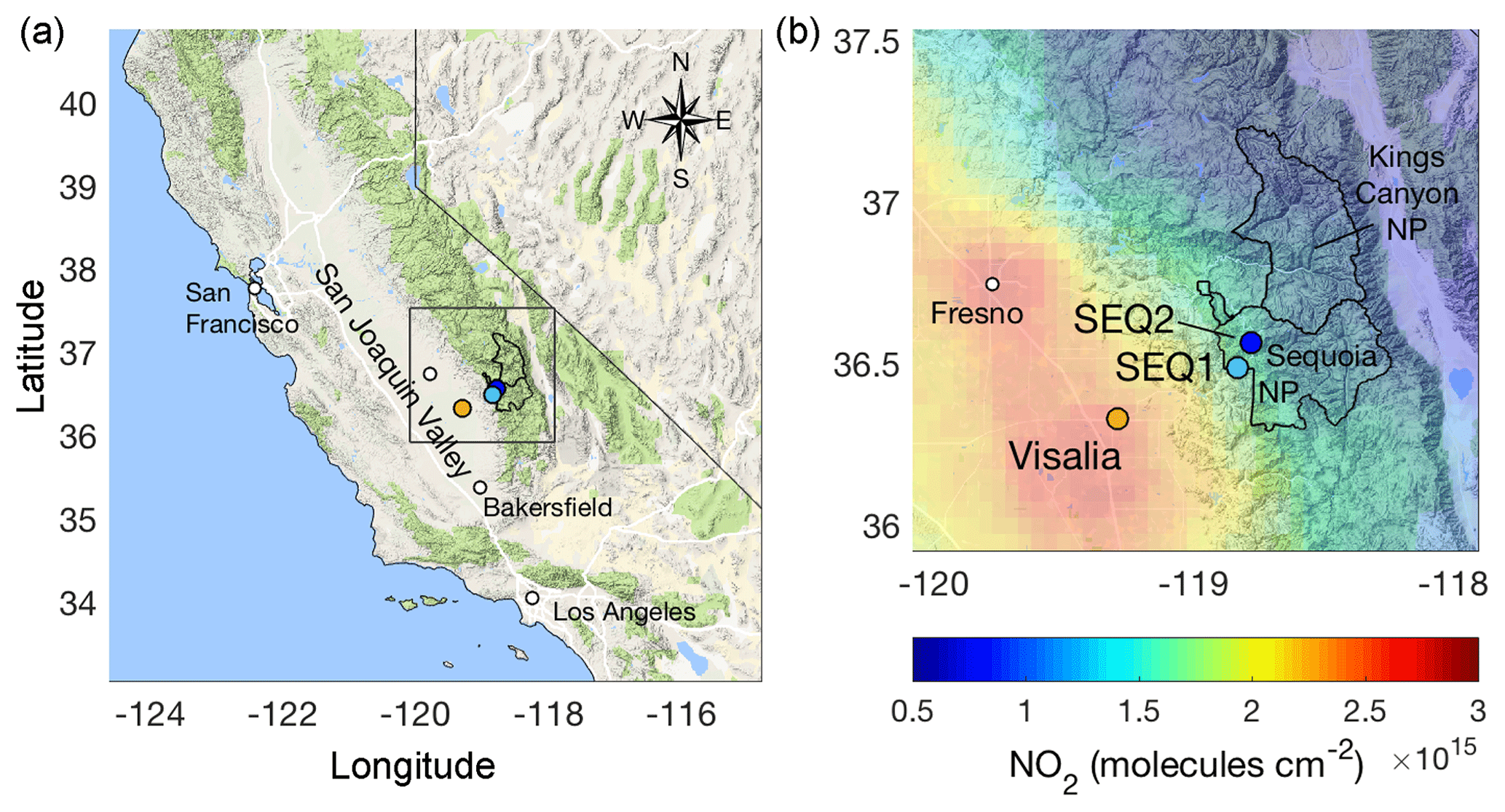
Figure 1Map of California (a) with study region detail (b) indicating the locations of the SJV station, Visalia (orange), and two monitoring sites in SNP, SEQ1 (cyan) and SEQ2 (dark blue), with mean April–October 2010–2012 OMI NO2 columns using the BEHR (Berkeley High-Resolution) product (Russell et al., 2011).
SNP is home to more than 1550 plant taxa with numerous plant species found nowhere else on Earth (Schwartz et al., 2013). One endemic species is the giant sequoia (Sequoiadendron giganteum), the largest living tree in the world. Large-tree ecosystems like SNP have been shown to be more sensitive to perturbation (Lutz et al., 2012) because ecological functions are provided primarily by a few large trees, rather than many smaller species. Large-diameter trees disproportionately influence patterns of tree regeneration and forest succession (Keeton and Franklin, 2005), carbon and nutrient storage, forest structure and fuel deposition at death, arboreal wildlife habitats and epiphyte communities (Lutz et al., 2012), and water storage (Sillett and Pelt, 2007), which is of critical importance in drought-prone SNP. While mature sequoias are relatively resistant to O3, seedlings are sensitive, with high O3 demonstrated to cause both visible injury and altered plant–atmosphere light and gas exchange (Miller et al., 1994). Giant sequoias grow in mixed conifer groves with companion species ponderosa pine (Pinus ponderosa) and Jeffrey pine (Pinus jeffreyi). O3 impacts on these pines have been documented for decades in SNP (Duriscoe, 1987; Pronos and Vogler, 1981) and include early needle loss, reduced growth, decreased photosynthesis, and lowered annual ring width (Peterson et al., 1987, 1991).
SNP is located in central California on the western slope of the Sierra Nevada Mountains downwind of the O3-polluted San Joaquin Valley (SJV) (Fig. 1). Previous model estimates of a pollution episode in August 1990 suggest at least half of peak daytime O3 in SNP is produced upwind from anthropogenic precursors (Jacobson, 2001). For the past 2 decades, regulations have reduced O3 concentrations in the SJV (Pusede and Cohen, 2012). For example, in Fresno, high O3 days, defined as days when the MD8A exceeds 70 ppb, were 50 % less frequent in 2007–2010 than 10 years earlier (on high temperature days). At the same time, in Bakersfield, high O3 days were 15 %–40 % less frequent (on high temperature days). NOx emission controls contributed to these decreases (Pusede and Cohen, 2012), with summertime (April–October) daytime (10:00–15:00 LT, local time) nitrogen dioxide (NO2) concentrations falling by 50 % from 2001 to 2012, changing linearly by −0.5 ppb yr−1 in the SJV city of Visalia. The precursor reductions that brought about these decreases in high O3 are likely to have also affected O3 in SNP.
The success of O3 regulatory strategies can be measured through the attainment of human-health-based NAAQS and ecosystem-impact metrics. While there is a secondary NAAQS requirement aimed at vegetation protection, this has historically been the same metric (based on the MD8A O3) at the same threshold as the primary NAAQS (Environmental Protection Agency, 2015b). Plants and ecosystems have been shown to be sensitive to lower O3 concentrations over longer-term exposures and at different times of day and year than when NAAQS exceedances are frequent (e.g., Kurpius et al., 2002; Panek, 2004; Panek and Ustin, 2005; Fares et al., 2013). While trends toward median O3 levels observed at a large number of US sites (Lefohn et al., 2017) may have decreased the number of NAAQS exceedances, benefits to plants and ecosystems may be limited (Lefohn et al., 2018). The U.S. Environmental Protection Agency (EPA) has considered redefining the secondary standard to reflect ecological systems, with the W126 metric put forth (Environmental Protection Agency, 2010). W126 is a 12 h daily 3-month summation weighted to emphasize higher O3 concentrations (Environmental Protection Agency, 2006, 2016) that is used by the U.S. National Park Service. There are a number of other concentration metrics used to quantify ecosystem O3 impacts. In Europe, the AOT40 index is common and is equal to all daytime (defined as solar radiation ≥50 W m−2) hourly O3 concentrations greater than 40 ppb. In the US, two widely used indices are the SUM0 and SUM06 (e.g., Panek et al., 2002), which are the sum of all daytime hourly O3 mixing ratios greater than or equal to 0 and 60 ppb, respectively. Similarly, the M12 metric is an average exposure metric computed over the same daily time window (08:00–20:00 LT) and representing the same hourly O3 concentrations when computed over a 3-month period as SUM0 (e.g., Tingey et al., 1991; Lefohn and Foley, 1993). For a global assessment of O3 distribution and trends using a variety of ecosystem concentration metrics, see Mills et al. (2018), which is part of the Total Ozone Assessment Report (TOAR).
Even ecosystem-based concentration metrics are proxies of variable quality for O3 impacts if O3 concentrations are not well correlated with plant O3 uptake (e.g., Emberson et al., 2000; Panek et al., 2002; Panek, 2004; Fares et al., 2010a). This is because of temporal mismatches between when O3 is high and when plants uptake O3 from the atmosphere, with differences in high O3 and efficient O3 uptake occurring on both diurnal and seasonal timescales. While ecosystem O3 impacts are best represented by direct measurements of the O3 stomatal flux (e.g., Musselman et al., 2006; Fares et al., 2010a, b), exceedances of flux-based standards are difficult to operationalize, as there are few long-term O3 flux observational records and because reported thresholds, when available, are highly species specific (Mills et al., 2011).
Under the 1977 Clean Air Act Amendments, selected national parks were designated as Class I Federal areas and, as part of this, the National Park Service began measuring O3 concentrations in the 1980s, prioritizing national parks downwind of cities and polluted areas, including SNP (National Park Service, 2015b). Data from these monitors can be used to compute various O3 concentration metrics; however, direct flux measurements do not exist in SNP, or other national parks, over long enough timescales to assess the effects of multiyear emissions controls. Forest survey data, which assess O3 impacts by monitoring changes in plants and forests from visible injury records and species population estimates, are limited, as they are labor and time intensive, requiring the evaluation of at least dozens of trees per stand to distinguish moderate levels of injury (Duriscoe et al., 1996). These studies occur at some time interval after exposure, making correlation with specific O3 concentrations not possible. As a result, there is a need to assess trends using concentration metrics, but to do so with knowledge of when plant O3 uptake is greatest.
In this paper, we report O3 trends from 2001 to 2012 in SNP and the upwind SJV city of Visalia to study the effects of SJV emission controls on SNP O3. We do not extend the analyses beyond 2012 as, beginning in late 2012, California experienced the worst drought in recorded history (Griffin and Anchukaitis, 2014; Diffenbaugh et al., 2015). Because O3 concentrations are influenced by drought conditions (e.g., Jacob and Winner, 2009; Huang et al., 2016), we focus on the 2001 to 2012 time period. We compute trends in human-health- and ecosystem-based concentration metrics separately when regional environmental conditions favor plant O3 uptake (springtime) and when high O3 is most frequent (O3 season). We describe these O3 changes in Visalia and SNP as a function of distance downwind of Visalia by way of data collected at two monitoring stations located on the western slope of the Sierra Nevada Mountains. We demonstrate the importance of the transport of urban NOx from the SJV to trends in O3 production (PO3) chemistry in SNP. Finally, we discuss the descriptive power of various O3 metrics and consider the implications of a regulatory focus on human-health-based standards to reduce ecosystem O3 impacts in SNP.
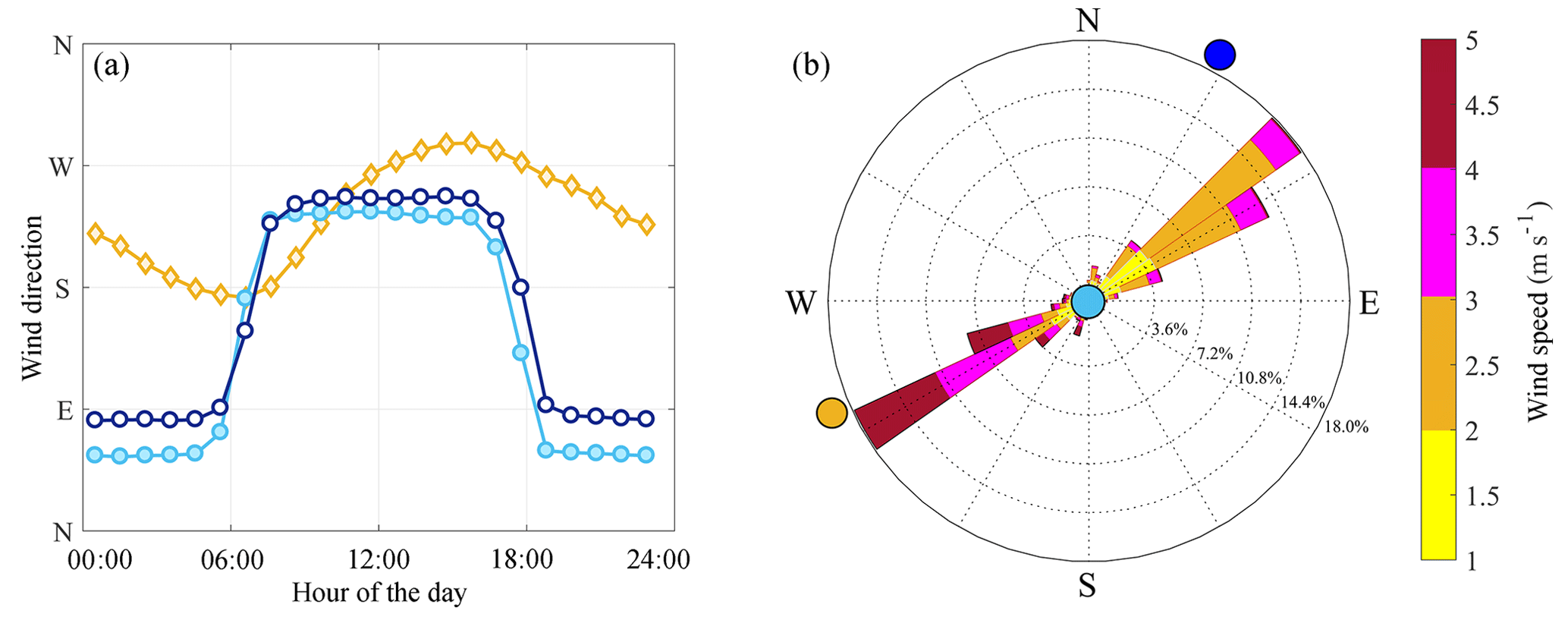
Figure 2Hourly mean wind directions in Visalia (orange diamonds), SEQ1 (cyan filled circles), and SEQ2 (dark blue open circles) in April–October 2001–2012 (a). Wind rose for SEQ1 (b) with the direction of the neighboring sites of Visalia (orange), SEQ1 (cyan), and SEQ2 (dark blue) indicated.
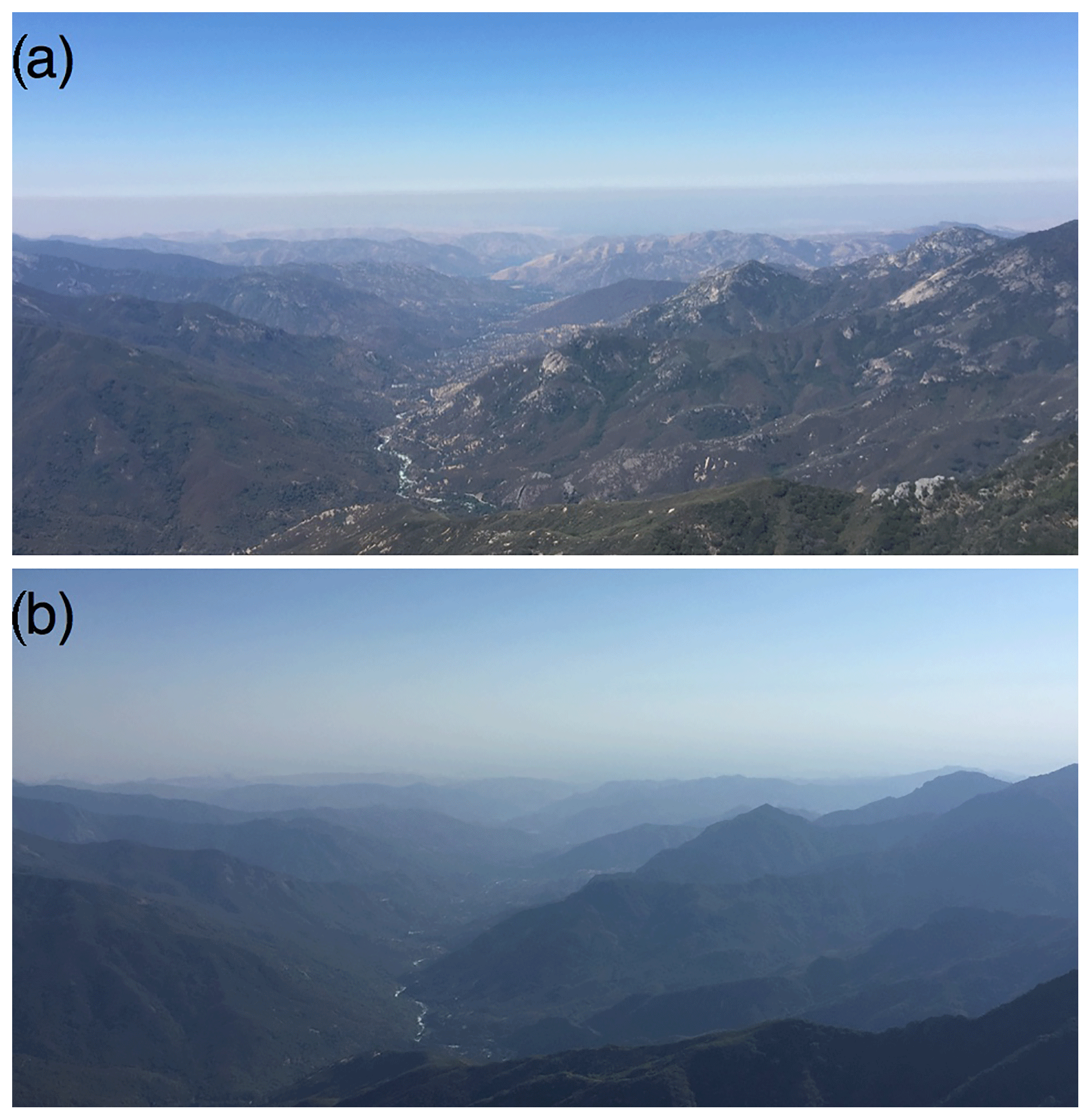
Figure 3Looking toward the SJV from Moro Rock in SNP (36.5469∘ N, 118.7656∘ W; 2050 ) at 11:00 LT (a) and 17:30 LT (b). Photographs were taken by the authors on 29 June 2017.
SNP is located in the southern Sierra Nevada Mountains (Fig. 1) and is part of the largest continuous wilderness in the contiguous US, which includes Kings Canyon NP and Yosemite NP. The SJV extends 400 km in length and is situated between the Southern Coast Ranges to the west, the Sierra Nevada Mountains to the east, and the Tehachapi Mountains to the south. The southern SJV is the most productive agricultural region in the US; it is also an oil and gas development area home to the cities of Fresno, Visalia, and Bakersfield. The same climatic conditions that support agriculture in the region, especially the numerous sunny days, are also favorable for PO3. The high rates of local PO3 (Pusede and Cohen, 2012; Pusede et al., 2014), diverse local emission sources outside historical regulatory focus, e.g., agricultural and energy development activities (e.g., Gentner et al., 2014a, b; Pusede and Cohen, 2012; Park et al., 2013), and surrounding mountain ranges that impede airflow out of the valley have resulted in severe regional O3 pollution. Four SJV cities rank among the 10 most O3-polluted cities in the US: Bakersfield (ranked 2), Fresno (3), Visalia (4), and Modesto–Merced (6) (American Lung Association, 2016).
Multiple airflow patterns influence O3 in SNP and the SJV (see Zhong et al., 2004, for a diagram). First, summertime (April–October) afternoon low-level winds in the southern SJV are generally from the west–northwest (represented by Visalia in Fig. 2a). These winds are strengthened by an extended land–sea breeze, with onshore flow entering central California through the Carquinez Strait near the San Francisco Bay and diverging to the south into the SJV and north to the Sacramento Valley (e.g., Zaremba and Carroll, 1999; Dillon et al., 2002; Beaver and Palazoglu, 2009; Bianco et al., 2011). Second, at night, a recurring local flow pattern in the SJV, known as the Fresno eddy, recirculates air in the southern region of the valley around Bakersfield in the counterclockwise direction back to Fresno and Visalia, further enhancing O3 pollution and precursors in these cities (e.g., Ewell et al., 1989; Beaver and Palazoglu, 2009). Third, the most populous and O3-polluted cities in the southern SJV, Fresno, Visalia, and Bakersfield, are located along the eastern valley edge. Here, air movement is also affected by mountain valley flow (e.g., Lamanna and Goldstein, 1999; Zhong et al., 2004; Trousdell et al., 2016). During the day, thermally driven upslope flow brings air from the valley floor to higher mountain elevations from the west–southwest (Fig. 2). In Fig. 3, a high-elevation SNP site (Moro Rock; 36.5469∘ N, 118.7656∘ W; 2050 m a.s.l.) is visibly above the SJV surface layer in the late morning, but within this polluted layer in late afternoon. At night, the direction of flow reverses and air moves downslope from the east–northeast (Fig. 2). The prevalence of shallow nighttime surface inversions in the SJV means that evening downslope valley flow at higher elevations may be stored within nocturnal residual layers and entrained into the surface layer the following morning.
High O3 days are most frequent in SNP and the SJV in the summer through early fall (Pusede and Cohen, 2012; Meyer and Esperanza, 2016), as PO3 chemistry is often temperature dependent (reviewed in Pusede et al., 2015) and this effect is particularly strong in the SJV (Pusede and Cohen, 2012; Pusede et al., 2014). The O3 season is defined here as June–October with ∼90 % of annual O3 8 h NAAQS exceedances in SNP occurring during O3 season (2001–2012).
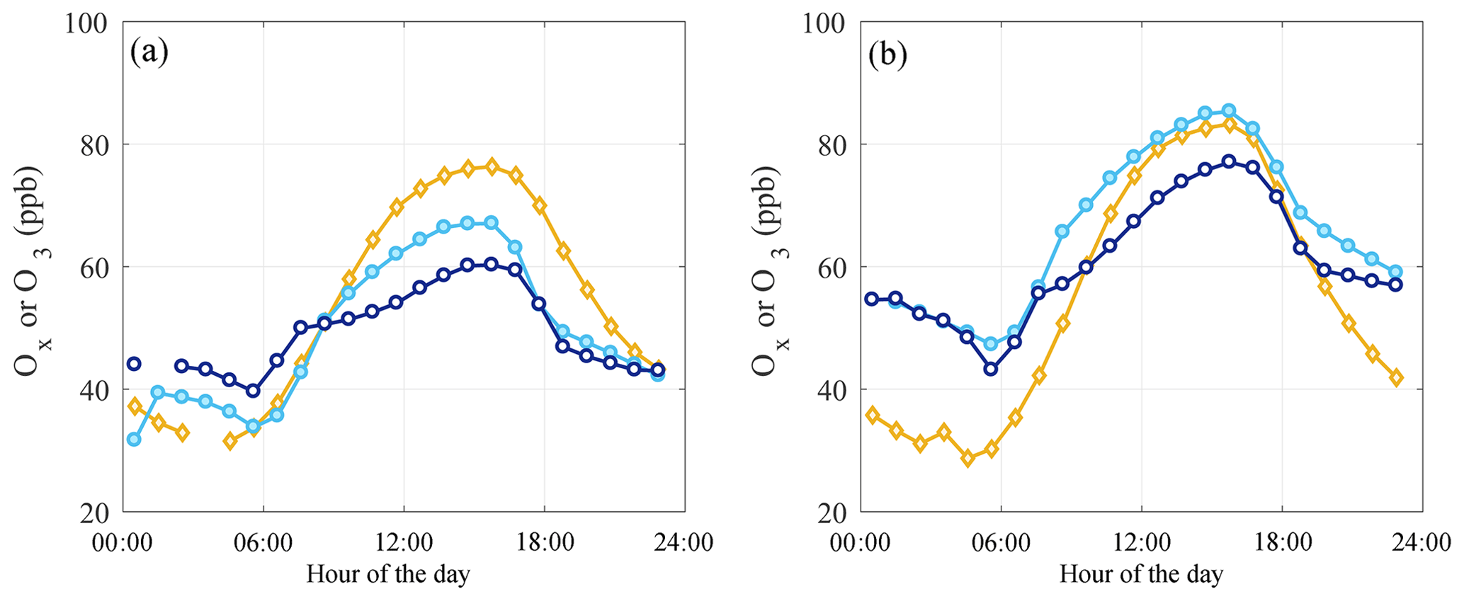
Figure 4Hourly mean Ox in Visalia (orange diamonds), SEQ1 (cyan filled circles), and SEQ2 (dark blue open circles) in springtime (a) and during the O3 season (b) 2001–2012. Data gaps are due to routine calibrations.
In the Sierra Nevada foothills, high rates of plant O3 uptake are asynchronous with O3 season because of the Mediterranean climate (e.g., Kurpius et al., 2002, 2003; Panek, 2004). Plants also capture carbon dioxide required for photosynthesis and transpire through stomata; therefore, O3 uptake is not only a function of the atmospheric O3 concentration, but also of photosynthetically active radiation (PAR), the inverse of the atmospheric vapor pressure deficit (VPD) (Kavassalis and Murphy, 2017), and soil moisture (e.g., Reich, 1987; Bauer et al., 2000; Fares et al., 2013). In SNP, PAR is highest in the late spring through early fall and VPD is at a minimum in winter and spring. In the Sierra Nevada Mountains, plant water status (VPD and soil moisture) has been shown to explain up to 80 % of day-to-day variability in stomatal conductance, with conductance decreasing with increasing water stress from mid-May to September and remaining low until soils are resaturated by wintertime precipitation. Plant O3 uptake in Sierra Nevada forests has been reported to be greatest in April–May (Kurpius et al., 2002; Panek, 2004; Panek and Ustin, 2005).
In this context, we separately consider O3 trends in springtime (April–May), which is when plant O3 uptake best correlates with variability in atmospheric O3 concentrations in the region, and during O3 season (June–October), which is when O3 concentrations are highest. In this paper, for clarity we generally use the term impacts when discussing ecosystem metrics and concentrations when talking about human health metrics; O3 ecosystem and human health effects are of course both O3 impacts.
Hourly O3 data have been routinely collected in SNP at two monitoring stations: a lower-elevation site, SNP Ash Mountain (36.489∘ N, 118.829∘ W) at 515 m above sea level (a.s.l.), and a higher-elevation site, SNP Lower Kaweah (36.566∘ N, 118.778∘ W) at 1926 m a.s.l. (Fig. 1). We refer to these stations as SEQ1 and SEQ2, respectively. O3 and NO2 data are measured in Visalia (36.333∘ N, 119.291∘ W), which is in the upwind direction of SNP at 102 m a.s.l. (Fig. 2). The data are collected by various agencies, including the National Park Service, hosted by the California Air Resources Board, and available for download at https://www.arb.ca.gov/aqmis2/aqdselect.php, last access: 6 July 2016.
3.1 Diurnal O3 variability
Diurnal O3 and Ox () concentrations are shown in Fig. 4 in springtime (panel a) and O3 season (panel b) over the 2001–2012 time period. Visalia data are shown as Ox to account for the portion of O3 stored as NO2, which can be substantial in the near field of fresh NOx emissions and at night. NO2 data are not available in SEQ1 and SEQ2; however, these sites are removed from large NOx sources (Fig. 1) and O3≈Ox is a reasonable approximation.
In Visalia, Ox concentrations increase sharply beginning in early morning (07:00 LT) until 14:00 LT, continuing to rise slightly until 16:00–17:00 LT (Fig. 4). This diurnal pattern reflects a combination of local PO3 (the initial rise) and advection of Ox from the upwind source region (late afternoon maximum). In the morning, enhanced rush-hour NOx emissions overlap in time with the initial increase in Ox with 30 %–40 % of Ox as NO2 at 07:00–08:00 LT. In the afternoon, from 12:00–16:00 LT ∼10 %–15 % of Ox is NO2. At 17:00, NO2 concentrations increase with evening rush hour with 30 %–40 % of Ox as NO2 at 17:00–18:00 LT.
Diurnal O3 variability at SEQ1 and SEQ2 is characterized by two features, an early morning rise (06:00 LT) and an increase in the late afternoon (15:00–16:00 LT). The timing of this morning O3 increase is consistent with entrainment of O3 in nocturnal residual layers aloft during morning boundary layer growth. The influence is substantial, as morning O3 accounts for 50 % (springtime and O3 season) of the daily change in O3 at SEQ1 and 50 % (springtime) and 37 % (O3 season) of the daily change in O3 at SEQ2. The timing of afternoon peak O3 is consistent with upslope air transport from the SJV (Fig. 2). If O3 attributed to local PO3 in Visalia is greatest around 14:00, typical of many urban locations, with mean winds at SEQ1 of 3 m s−1 and SEQ2 of 2 m s−1, we expect O3 to peak in SEQ1 at approximately 17:00 LT (45 km downwind of Visalia) and at SEQ2 shortly after (9.7 km downwind of SEQ1, which includes the change in elevation using the Pythagorean theorem). This is broadly what we observe. While the actual distance of airflow is dictated by the mountain terrain and a parcel of air will travel a distance longer than the straight-line path on a smooth surface, the timing of the O3 diurnal patterns is consistent with airflow travel time roughly equal to that determined by the horizontal distance and mean wind speed. There has been no change in the hour of peak O3 mixing ratio at either SEQ1 or SEQ2 over the 2001 to 2012 period.
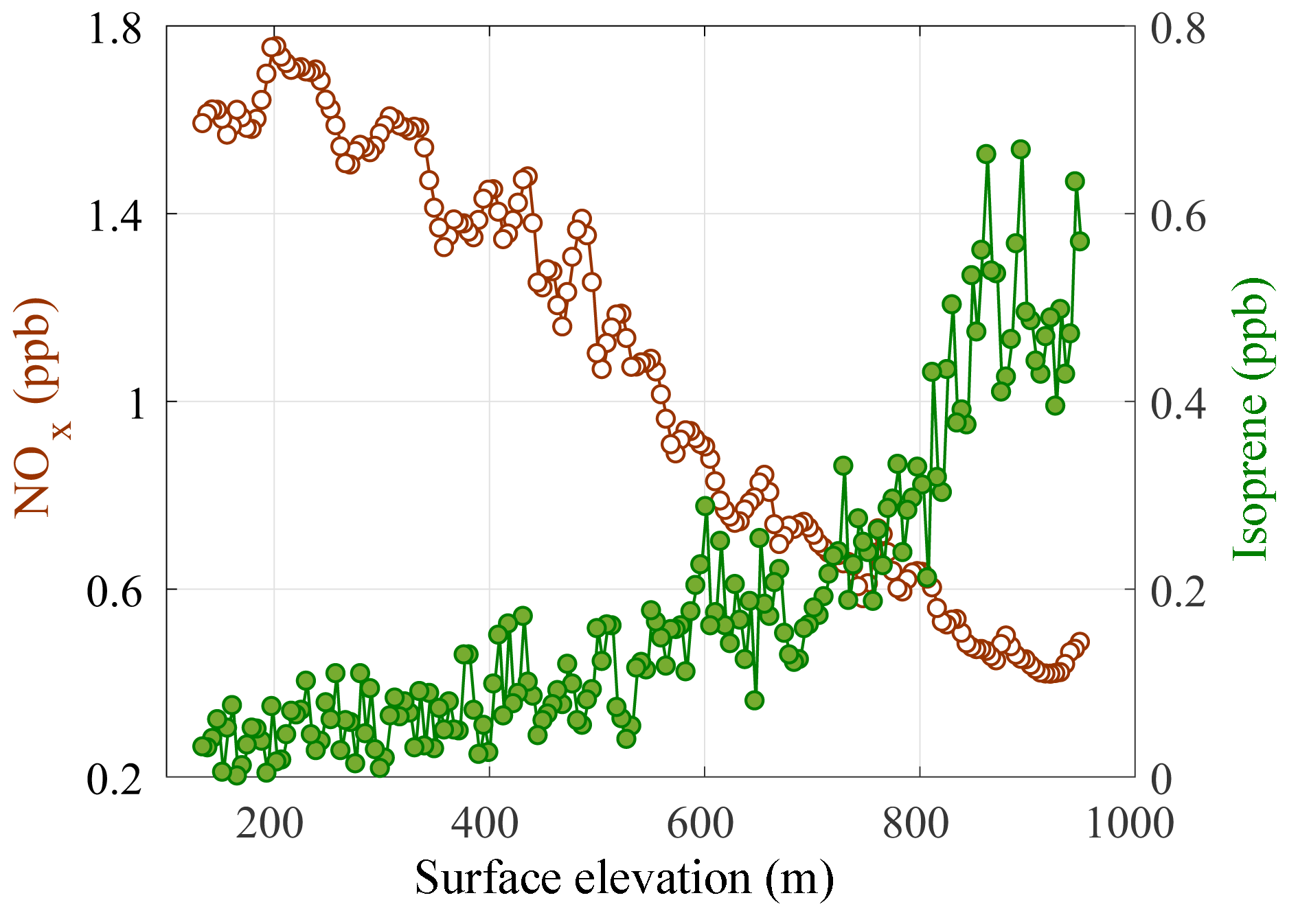
Figure 5NOx (brown open circles) and isoprene (green filled circles) measured onboard the NASA DC-8 at ∼10:00 LT at the Sierra Nevada western slope from a mean altitude of 130 to 1000 on 19 June 2016. The surface elevation is estimated by linearly interpolating across the total elevation change.
3.2 Weekday–weekend O3 variability
SNP and the SJV are in close geographic proximity but their local PO3 regimes are different. In 2016, as part of the Korea–US Air Quality (KORUS-AQ) experiment (https://www-air.larc.nasa.gov/missions/korus-aq/index.html, last access: 8 July 2016) and Student Airborne Research Program (SARP), the NASA DC-8 sampled a low-altitude transect (∼130 m above ground level) along the trajectory of SJV mountain valley outflow. The DC-8 flew at ∼10:00 LT from Orange Cove, an SJV town 35 km north of Visalia, 24 km up the western slope of the Sierra Nevada Mountains to an elevation of ∼1000 m a.s.l. In Fig. 5, the change in NOx and isoprene along this transect is shown as a function of change in surface elevation. Boundary layer NOx is observed to decrease with increasing distance downwind of the SJV, while isoprene concentrations increase. Isoprene is a large source of reactivity in the Sierra Nevada foothills (e.g., Beaver et al., 2012; Dreyfus et al., 2002) and the combined NOx and isoprene gradients suggest potentially distinct PO3 regimes in the SJV and SNP. While these data were collected on one day in a different year from our study, the relative pattern of NOx to organic compound emissions is likely representative, as there have been no substantial changes in the locations of urban NOx and biogenic organic emitters. This NOx to organic compound gradient is consistent with observations over longer sampling periods downwind of the central California city of Sacramento, where the NOx-enriched Sacramento urban plume is transported up the western slope of the vegetated Sierra Nevada Mountains (e.g., Beaver et al., 2012; Dillion et al., 2002; Murphy et al., 2006).
If the major source of O3 in SNP is O3 produced in the SJV and transported downwind, then the observed NOx dependence of PO3 in SNP and the SJV would be the same even if PO3 regimes in the two locations were different. To test this hypothesis, we consider O3 in SNP and Ox in the SJV separately on weekdays and weekends. Weekday–weekend NOx concentration differences are well documented across the US (e.g., Russell et al., 2012) and California (e.g., Marr and Harley, 2002; Russell et al., 2010) and are caused by reduced weekend heavy-duty diesel truck traffic; heavy-duty diesel trucks are large sources of NOx but not O3-forming organic gases. As a result, NOx concentrations are typically 30 %–60 % lower on weekends than weekdays and these NOx changes occur without comparably large decreases in reactive organic compounds (e.g., Pusede et al., 2014). PO3 is the only term in the O3 derivative expected to exhibit NOx dependence.
We focus on the earliest 3-year time period in our record, 2001–2003, which is when differences in PO3 chemical sensitivity in the SJV and SNP are expected to be most pronounced (Pusede and Cohen, 2012). We define weekdays as Tuesdays–Fridays and weekends as Sundays to avoid atmospheric memory effects. Statistics were sufficient to minimize any co-occurring variation in meteorology, with no significant weekday–weekend differences observed in daily maximum temperature, wind speed, or wind direction. We focus on afternoon (12:00–18:00 ) Ox, when O3 concentrations in SNP are most influenced by the SJV (from Fig. 4). We also compare weekday–weekend Ox at high and moderate temperatures, with temperature regimes defined as days above and below the 2001–2012 seasonal mean daily maximum average temperature in Visalia. Temperatures in Visalia are well correlated (R2=0.98) with temperatures in SEQ1 over 2001–2012. During springtime and O3 season, mean maximum average temperatures in Visalia were 25.1±5.9 and 32.0±5.3 ∘C (ranges are 1σ variability), respectively.
Table 1Percent difference in afternoon (12:00–18:00 LT) Ox or O3 on weekdays and weekends calculated as in Visalia, SEQ1, and SEQ2 in 2001–2003 on moderate and high temperature days. Errors are reported as standard errors of the mean.
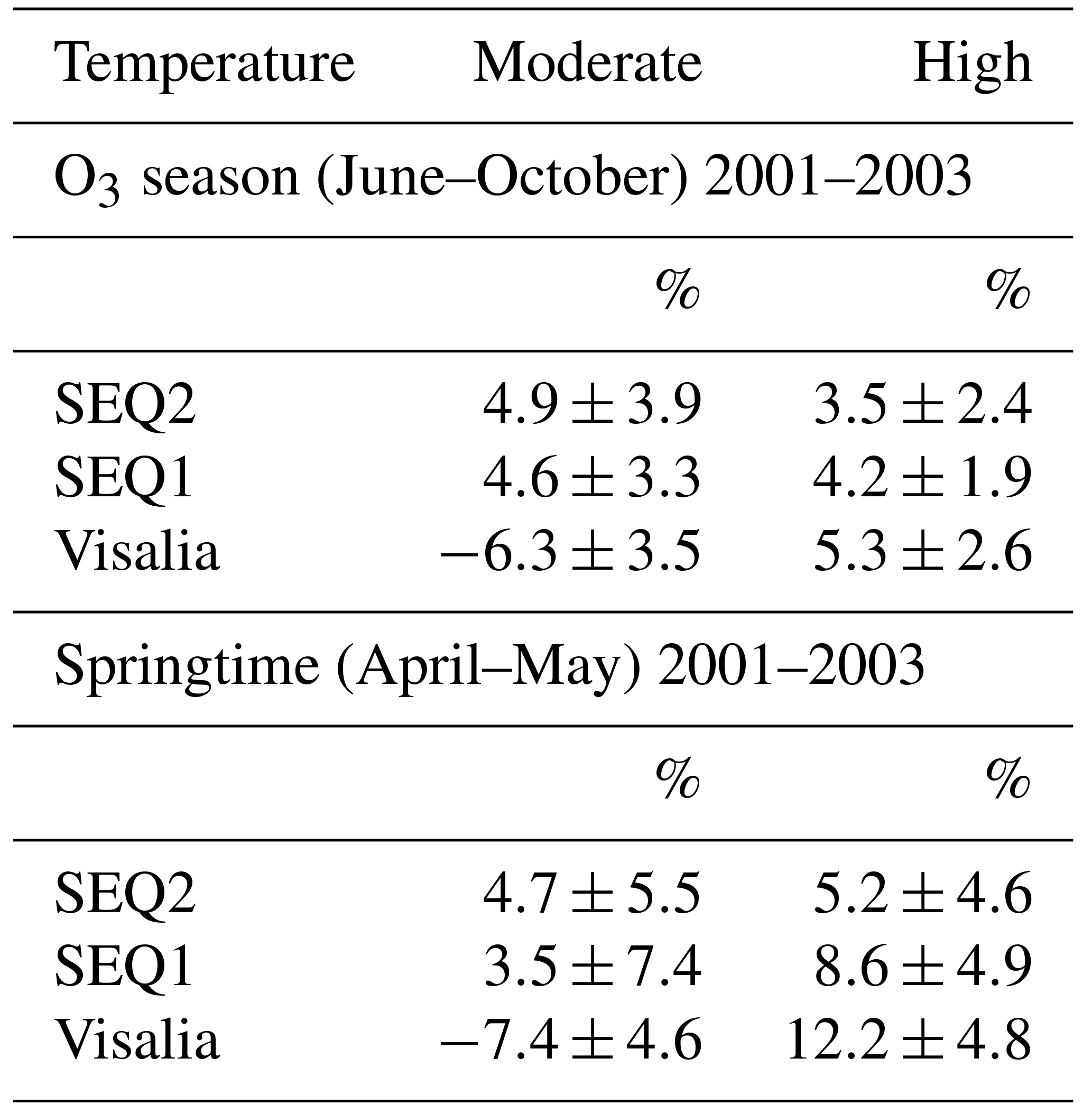
At moderate temperatures, statistically significant weekday–weekend differences were observed (Table 1). During O3 season, Ox was 6.3±3.5 % higher on weekends than weekdays (relative to weekdays) in Visalia, indicating local PO3 was NOx suppressed. At the same time, O3 was 4.6±3.3 % and 4.9±3.9 % higher on weekdays than weekends at SEQ1 and SEQ2, respectively, implying PO3 in SNP was NOx limited. A similar pattern was observed during springtime, as Ox was 7.4±4.6 % higher on weekends than weekdays in Visalia and O3 was 3.5±7.4 % and 4.7±5.5 % higher on weekdays than weekends in SEQ1 and SEQ2. These weekday–weekend patterns imply that a substantial portion of O3 in SNP is produced by low NOx–PO3 chemistry during air transport from the SJV. At high temperatures, greater weekday concentrations in Ox in Visalia and O3 at SEQ1 and SEQ2 imply NOx-limited chemistry in all three locations (Table 1). Averaged across sites, percent differences in weekdays and weekends were 8.7±4.8 % in the springtime and 4.3±2.3 % during O3 season. PO3 during upslope transport is not apparent by this method because O3 season PO3 was also NOx limited in Visalia, indicating a portion of O3-forming organic reactivity in Visalia was temperature dependent, consistent with past analyses in other SJV cities (Steiner et al., 2006; Pusede and Cohen, 2012; Pusede et al., 2014; Rasmussen et al., 2013).
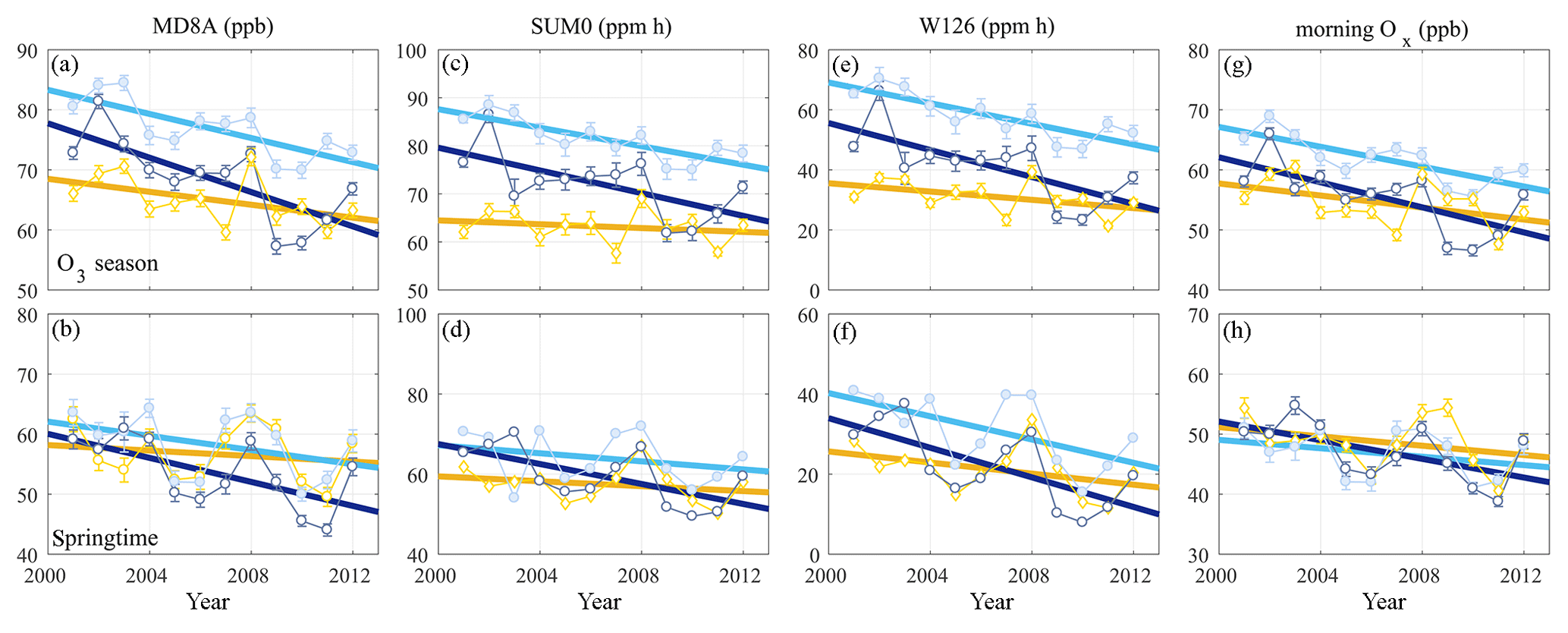
Figure 6O3 trends in Visalia (orange diamonds), SEQ1 (cyan filled circles), and SEQ2 (dark blue open circles) computed using MD8A (a–b), SUM0 (c–d), W126 (e–f), and morning Ox (g–h) metrics during O3 season (a, c, e, g) and springtime (b, d, f, h). Both MD8A and morning Ox are computed as seasonal averages. Error bars in (a)–(b) and (g)–(h) are standard errors of the mean. Error bars in (c) and (e) are standard errors of the mean of the three O3 season 3-month summations.
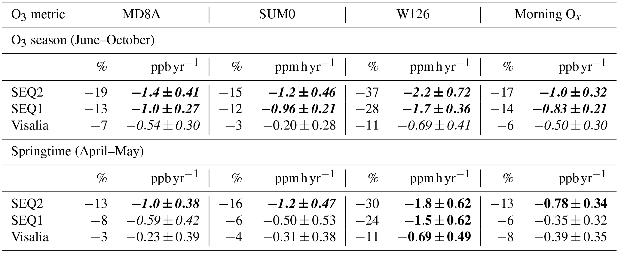
Table 2O3 changes in Visalia, SEQ1, and SEQ2 over 2001–2012 according to MD8A, SUM0, W126, and morning Ox metrics based on a linear fit of annual mean data (shown in Fig. 6) in the springtime and O3 season. Each left column is the percent change with respect to fit value in 2001 at SEQ1 during O3 season for comparison, which is the highest O3 observed for each metric. Each right column is the fit slope with slope errors in O3 abundance units per year. Font style is based on the TOAR categorization for trend significance (Lefohn et al., 2018), with p values calculated using the Mann–Kendell nonparametric test: bold italics, 0–0.05, statistically significant trend; bold, 0.05–0.10, indicative of a trend; italics, 0.10–0.34, weak indication of change; and normal font, 0.34–1, weak or no change.
3.3 O3 trends over time
In Fig. 6 and Table 2, we report 12-year O3 trends (2001–2012) in SNP and the SJV in springtime and during O3 season using four concentration metrics: MD8A; two common vegetative-based indices, SUM0 and W126; and a morning average metric. We do not report trends in SUM06 or AOT40 vegetative indices, as they have been shown to poorly correlate with O3 uptake at a Sierra Nevada forest site even in springtime (Panek et al., 2002; Fares et al., 2010b). MD8A O3 is a human-health-based metric computed as the maximum unweighted daily 8 h average O3 mixing ratio. A region is classified as in nonattainment of the NAAQS when the fourth-highest MD8A O3 over a 3-year period, known as the design value, exceeds a given standard. In this work, we utilize the seasonal mean MD8A and discuss O3 exceedances as individual days on which MD8A O3>70.9 ppb, the current 8 h NAAQS (Code of Federal Regulations 40, 2015). SUM0 is equal to the sum of hourly O3 concentrations over a 12 h daylight period (08:00–20:00 LT), as opposed to SUM06, which is limited to hourly O3 mixing ratios greater than 60 ppb. SUM0 is based on the assumption that the total O3 dose has a greater impact on plants than shorter-duration high O3 exposures (Kurpius et al., 2002). The summation is unweighted, attributing equal significance to high and low O3 concentrations (Musselman et al., 2006). SUM0 averaging is restricted to time periods when stomata are open (daylight), a condition not required for the MD8A. W126 is a weighted summation (08:00–20:00 LT), assuming higher O3 is more damaging to plants than lower O3 levels. W126 weighting is sigmoidal, with hourly O3 weights equal to such that hourly mixing ratios below (above) 60 ppb receive less (more) weight (Environmental Protection Agency, 2016). Here, SUM0 and W126 summations are computed following the W126 protocol (Environmental Protection Agency, 2016), affording straightforward comparisons between the metrics. First, in months with less than 75 % of hourly data coverage in the 08:00–20:00 LT window, missing values are replaced with the lowest observed hourly measurement over the study period (April–October) only until the dataset is 75 % complete. From 2001–2012, 0, 8, and 3 months were initially less than 75 % complete in Visalia, SEQ1, and SEQ2, respectively. Second, monthly summations of daily indices comprised of hourly data (08:00–19:00 LT) are computed; when data are missing, the summation is divided by the data completeness fraction. Consecutive 3-month metrics are computed by adding monthly indices. In practice, SUM0 and W126 are computed as 3-year averages of the highest 3-month summation; however, we define springtime SUM0 and W126 as the 3-month summation over April–June and O3 season SUM0 and W126 as the mean of the 3-month summations over June–August, July–September, and August–October (not the highest of the three 3-month sums). Because less than 15 % of data were available for August 2008 at SEQ1, O3 season SUM0 and W126 were computed as the mean of 3-month summations over June, July, and September and July, September, and October only for this site and year. We compute morning (07:00–12:00 LT) trends (Ox in Visalia and O3 in SNP), as high O3 plant uptake rates (in the morning) and high O3 concentrations (in the afternoon) are out of phase within daily timeframes in the Sierra Nevada Mountains. Plant O3 uptake typically follows a pattern of rapid morning uptake, relatively constant flux through midday, and a decrease in uptake in afternoon as plants close their stomata to prevent water loss in the hot, dry afternoon (Kurpius et al., 2002; Fares et al., 2013). Efficient morning uptake occurs because plants recharge their water supply overnight, which with low morning temperatures and VPD results in high stomatal conductance (Bauer et al., 2000). Morning uptake in the Sierra Nevada maximizes in springtime around 08:00 LT (Kurpius et al., 2002; Panek and Ustin, 2005; Fares et al., 2013).
In Fig. 6, mean seasonal daily MD8A and morning metrics as well as cumulative SUM0 and W126 metrics are shown for Visalia, SEQ1, and SEQ2 with their fit derived using an ordinary least squares linear regression. Table 2 reports both the regression slope value (right columns) and the change in O3 relative to the O3 season fit value in SEQ1 in 2001 reported as a percent (left columns). SEQ1 experiences the highest O3 observed for each metric, and using a standard denominator facilitates comparison between monitoring sites and between seasons. Table 2 font style indicates trend significance computed using the Mann–Kendall nonparametric test following the categorization developed by TOAR authors (Chang et al., 2017; Mills et al., 2018; Lefohn et al., 2018), with p values deemed statistically significant (0–0.05) and indicative of a trend (0.05–0.10), weakly indicative of change (0.10–0.34), and indicative of weak or no change (0.34–1).
Three patterns emerge in SNP O3 trends over time: (1) O3 decreased everywhere over the 12-year record by all metrics in both seasons; (2) O3 decreased at a slower rate in the springtime than during O3 season by most metrics; and (3) O3 decreased more rapidly in SNP versus Visalia and at SEQ2 versus SEQ1.
Seasonal differences in O3 trends are prominent at each site. For example, O3 at SEQ1 generally decreased less in springtime than during O3 season (Table 2). For context in SEQ1, during O3 season the mean MD8A declined from 82.3 ppb (2001–2002) to 73.8 ppb (2011–2012), but in the springtime the MD8A fell from 61.7 ppb (2001–2002) to 55.6 ppb (2011–2012). SUM0 O3 fell from 87.0 ppm h (2001–2002) to 79.0 ppm h (2011–2012) during O3 season and from 69.9 ppm h (2001–2002) to 61.8 ppm h (2011–2012) in the springtime. W126 O3 decreased from 67.8 ppm h (2001–2002) to 53.7 ppm h (2011–2012) during O3 season and from 39.8 ppm h (2001–2002) to 25.4 ppm h (2011–2012) in springtime. Morning O3 fell from 67.1 ppb (2001–2002) to 59.6 ppb (2011–2012) during O3 season and from 49.0 ppb (2001–2002) to 45.1 ppb (2011–2012). This pattern was not observed in one instance: SUM0 in SEQ2. Here, seasonal differences were comparable; however, mean daily indices were observed to differ, and SUM0 O3 decreased from 0.914 ppm h (2001–2002) to 0.816 ppm h (2011–2011) during O3 season and in the springtime fell from 0.673 ppm h (2001–2002) to 0.616 ppm h (2011–2012), which amounts to a change of −11 % during O3 season and −8 % in the springtime.
Additionally, greater O3 decreases were observed at SEQ1 than Visalia and at SEQ2 compared to SEQ1. Over the 12-year period, MD8A O3 declined at a rate of 46 % (O3 season) and 61 % (springtime) faster at SEQ1 than in Visalia and 29 % (O3 season) and 41 % (springtime) faster at SEQ2 than SEQ1 (based on the slopes reported in Table 2). SUM0 and W126 O3 decreased 79 % and 59 % (O3 season) and 38 % and 54 % (springtime) faster at SEQ1 than in Visalia and 20 % and 23 % (O3 season) and 58 % and 17 % (springtime) faster at SEQ2 than SEQ1. Morning Ox trends at SEQ1 and Visalia were similar in springtime, but Ox decreased 40 % more rapidly at SEQ1 during O3 season and faster at SEQ2 than SEQ1 by 17 % (O3 season) and 55 % (springtime). For each metric, we observe greater interannual variability relative to the net decline in springtime than during O3 season. This site dependence is reflected in the O3 trend p values (Table 2): at SEQ2, slopes are either statistically significant at the 0.05 level or indicative of a trend (0.05–0.10) for each metric in both seasons. At SEQ1, slopes are statistically significant during O3 season, but only indicative (W126), weakly indicative (MD8A), or suggestive of weak to no change (SUM0 and morning Ox) in springtime. Trends in Visalia are the least robust, with p values typically only weakly indicative or suggestive of minor to no change in both springtime and O3 season.
High O3, as defined by exceedances of protective thresholds, also became less frequent over the 12-year record. The number of days in which MD8A O3 was greater than 70.9 ppb in 2001–2002 (averages are rounded up) was 66 yr−1 (O3 season) and 14 yr−1 (springtime) in Visalia. In 2011–2012, the number of exceedances fell to 39 yr−1 (O3 season) and 6 yr−1 (springtime). At SEQ1 in 2001–2002, there were 119 exceedance days yr−1 (O3 season) and 20 yr−1 (springtime), declining in 2011–2012 to 97 yr−1 (O3 season) and 10 yr−1 (springtime). At SEQ2 in 2001–2002, there were 103 exceedance days yr−1 (O3 season) and 13 yr−1 (springtime). In 2011–2012, this decreased to 62 exceedance days yr−1 (O3 season) and 3 yr−1 in 2011–2012 (springtime). Patterns in high MD8A O3 days follow trends in other metrics, with the largest rates of change occurring during O3 season in SEQ2 (−4.7 days yr−1, p=0.02), then SEQ1 (−2.8 days yr−1, p=0.05) and Visalia (−2.5 days yr−1, p=0.05). In springtime, smaller decreases are observed with similar spatial patterns for SEQ2 (−1.0 days yr−1, p=0.02), SEQ1 (−1.0 days yr−1, p=0.15), and Visalia (−0.5 days yr−1, p=0.37).
While there is no standard for SUM0, there are three time-integrated W126 protective thresholds. These are 5–9 ppm h to protect against visible foliar injury to natural ecosystems, 7–13 ppm h to protect against growth effects to tree seedlings in natural forest stands, and 9–14 ppm h to protect against growth effects to tree seedlings in plantations, known as the 5, 7, and 9 ppm h standards (Heck and Cowling, 1997). The EPA has considered a potential secondary W126 ozone standard between 7 and 17 ppm h (Environmental Protection Agency, 2015a); likewise, the Clean Air Science Advisory Committee recommended a W126 standard level between 7 and 15 ppm h (Environmental Protection Agency, 2015a). In this work, rather than calculate W126 exceedances using a 3-month summation of monthly indices, we instead count the number of days required for an exceedance to occur, summing daily W126 indices from the first day of springtime (1 April). A larger number of days indicates improved air quality. We do this to generate information in addition to exceedance frequency, as W126 O3 at SEQ1 and SEQ2 is greater than all three standards in all years in both seasons. We only consider springtime, as this is when W126 is reported to better correlate with plant O3 uptake (Panek et al., 2002; Kurpius et al., 2002; Bauer et al., 2000). At SEQ1 from 1 April in 2001–2002, 37, 41, and 45 days of O3 accumulation reached exceedances of the 5, 7, and 9 ppm h thresholds, respectively (averages are rounded up). In 2011–2012, 3 to 13 more days were needed at SEQ1, as 40, 49, and 58 days of O3 accumulation were required to exceed the 5, 7, and 9 ppm h thresholds. At SEQ2 from 1 April in 2001–2002, 41, 46, and 49 days of accumulation led to exceedance of the 5, 7, and 9 ppm h thresholds, respectively. In 2011–2012, 59, 65, and 73 days were required at SEQ2, or 18–24 more days.
4.1 O3 metrics
Long-term measurements of O3 fluxes rather than O3 concentrations are required to fully understand the effects of upwind emission controls on ecosystem O3 impacts. This is particularly true in Mediterranean ecosystems like SNP and under drought conditions, which is where and when plant O3 uptake and high atmospheric O3 concentrations may be uncorrelated (e.g., Panek et al., 2002). This may also be true in European Mediterranean climate regions, where high concentrations of ecosystem-based O3 metrics have also been observed (Mills et al., 2018). We have based our analysis on results from years of O3 flux data collected in forests on the western slope of the Sierra Nevada Mountains (Bauer et al., 2000; Panek and Goldstein, 2001; Panek et al., 2002; Kurpius et al., 2002; Fares et al., 2010a, b, 2013); however, there are few other O3 flux datasets that span multiyear timescales and no flux observations in SNP. In California, flux measurements suggest springtime SUM0 trends offer the most insight into trends in ecosystem O3 impacts in SNP; that said, we find similar conclusions would be drawn regarding multiyear O3 variability by location by assessing trends in SUM0, MD8A O3, and the morning Ox metric. This can be explained by the upslope–downslope airflow in our study region and is evident in SNP diurnal O3 patterns (Fig. 4), which show considerable O3 entrained into the boundary layer in the morning. O3 concentrations are strongly influenced by afternoon concentrations on the previous day. Comparable trends in morning, afternoon, and daily average O3 would then arise under conditions of persistence, which are common in central California, but these results may not extend to other downwind ecosystems in the absence of an upslope–downslope flow pattern. The dynamically driven elevated morning O3 concentrations have important consequences for plants, as vegetation in SNP may be particularly vulnerable because plant O3 uptake rates are often highest in the morning.
Reductions in ecosystem O3 impacts as represented by declines in W126 are greater than those of SUM0. We attribute this difference to the W126 weighting algorithm that makes the metric most sensitive to changes in the highest O3. Using the GEOS-Chem model with a focus on national parks, Lapina et al. (2014) also found W126 was more responsive to decreases in anthropogenic emissions than daily (08:00-19:00 LT) average O3 concentrations. With the Community Earth System Model, Val Martin et al. (2015) modeled air quality in national parks under two Representative Concentration Pathway (RCP) scenarios, computing substantially larger decreases over a 50-year period in W126 O3 compared to the MD8A. In the TOAR global analysis, Mills et al. (2018) found April–September W126 downward trends over 1995–2014 in California of 1–2 ppm h yr−1 to be among the most rapid W126 declines in the world. Considering that the SUM0 metric has been shown to best correspond to plant O3 uptake in Sierra Nevada forests using O3 flux observations (Panek et al., 2002) and that we observe W126 O3 has declined at approximately twice the rate of SUM0 over 2001–2012, W126 trends may provide an overly optimistic representation of past declines in ecosystem O3 impacts in SNP.
4.2 Reducing high O3 in SNP and polluted downwind ecosystems
NOx decreases have generally made greater improvements in O3 in SEQ1 than Visalia and in SEQ2 than SEQ1, a trend that corresponds to increasing distance downwind of the SJV. We attribute this to the importance of the export of NOx from the SJV for O3 in SNP, combined with distinct PO3 chemical regimes in SNP versus Visalia. Evidence for this is four-fold. First, O3 at SEQ1 is greater than Ox in Visalia, at least during O3 season, suggesting net O3 formation as air travels from the SJV to SNP. Second, according to observations of Ox (Visalia) and O3 (SNP) on weekdays versus weekends, PO3 was simultaneously NOx suppressed in Visalia and NOx limited in SNP, with the weekday–weekend dependence of O3 reflecting the chemical regime in which it is produced. Third, aircraft observations collected in the direction of daytime upslope flow from the SJV to the Sierra Nevada foothills reveal substantial decreases in NOx concentrations relative to isoprene, a key contributor to total organic reactivity (e.g., Beaver et al., 2012). Fourth, O3 decreases (2001–2012) are observed to be greater in SNP than Visalia and greater with increasing distance downwind. Distinct local PO3 regimes lead to PO3 chemistry in Visalia and SNP that is differently sensitive to emission controls, with NOx-limited SNP historically more responsive to NOx emission control than Visalia. SNP NOx limitation is enhanced by NOx dilution during transport, which further decreases NOx relative to the abundance of local organic compounds. Downwind sites usually experience PO3 chemistry that is more NOx limited than in the often NOx suppressed (or at least more NOx suppressed) urban core. As a result, we expect similar location-specific O3 trends in other ecosystems and national parks downwind of major NOx sources like cities. However, while the extent of observed O3 improvements in SNP follows the pattern of increasing distance downwind of Visalia with sustained NOx emission control in the SJV (Russell et al., 2010; Pusede and Cohen, 2012), PO3 chemistry is nonlinear and the direction of location-specific trends may vary. That said, at some distance downwind this conclusion breaks down as areas become less and less influenced by the upwind source.
Because PO3 in SNP is NOx limited, future NOx reductions are expected to have at least as large an impact on local PO3 as past reductions. Seasonal mean NO2 concentrations have decreased by 58 % and 53 % in Visalia in springtime and O3 season over our study window, respectively. Local NOx emissions should continue to decline into the future, as there are significant controls currently ongoing or in the implementation phase, including more stringent national rules on heavy-duty diesel engines (Environmental Protection Agency, 2000, 2007), combined with California Air Resources Board (CARB) diesel engine retrofit-replacement requirements (California Air Resources Board, 2008, 2014) and more stringent CARB standards for gasoline-powered vehicles (California Air Resources Board, 2007). While O3 declines near or greater than those that occurred from 2001 to 2012 are required to eliminate exceedances in SNP, modeling analysis by Lapina et al. (2014) suggests that W126 in the region would be well below these thresholds in the absence of anthropogenic precursor emissions, implying further emissions controls would be effective. Under the stringent precursor controls of RCP4.5, Val Martin et al. (2015) projected decreases of 11 % and 67 % for the MD8A and W126 in 2050, respectively, from the base year of 2000, with mean O3 decreasing from 58.9 ppb (MD8A) and 45.5 ppm h (W126) in 2000 to 52.7 ppb (MD8A) and 15.1 ppm h (W126). Under RCP8.5, smaller O3 declines were predicted, with MD8A unchanged and W126 falling by 38 % to 28.3 ppm h. Given that these scenarios represent a reasonable spread of possible future climatic conditions, Val Martin et al. (2015) suggest at least W126 will remain well above protective thresholds in 2050.
Over 2001–2012, O3 declines were mostly smaller in SNP when plant O3 uptake is greatest (springtime), despite comparable NOx decreases in both seasons. This may be in part because regulatory strategies prioritize attainment of the O3 NAAQS in polluted urban areas like the SJV basin, where air parcels influenced by the results of these controls are then transported downwind to locations with different PO3 chemistry. In the development of regulatory plans, agencies use models to hindcast past O3 episodes, facilitating testing of the efficacy of specific NOx and/or organic emissions reductions over that episode to meet the 8 h O3 NAAQS or progress goals (Environmental Protection Agency, 2007, 2014). In nonattainment areas, U.S. EPA guidance recommends modeling past time periods that meet a number of specific criteria, such as typifying the meteorological conditions that correspond to high O3 days as defined by the MD8A greater than the NAAQS value and focusing on the 10 highest modeled O3 days (Environmental Protection Agency, 2007, 2014). Regulatory modeling in the SJV (Visalia, SEQ1, and SEQ2 are included in this attainment demonstration) is more comprehensive, as it was recently updated to span the full O3 season (defined as May–September); still, potential reductions (known as relative reduction factors, RRFs) are based on the MD8A and restricted to high O3 days (San Joaquin Valley Unified Air Pollution Control District, 2007, 2016). In the SJV, high O3 days are most frequent in the late summer (O3 season) and on the hottest days of the year (Pusede and Cohen, 2012). Even in SEQ1 and SEQ2, days with MD8A >70.9 ppb are far more common in the summer. Because of chemical and meteorological differences between seasons, this may lead to policies not optimized to decrease O3 in cooler springtime conditions, which in the SJV are more NOx suppressed and therefore more sensitive to controls on reactive organic compounds (Pusede et al., 2014). In addition, we observe greater year-to-year O3 variability in the springtime than during O3 season (Fig. 6), suggestive of a larger relative role of interannual meteorological variability controlling O3 concentrations. Deeper cuts in emissions appear to be required in the springtime in SNP, as decreases in anthropogenic emissions have a smaller effect, both relatively and in the absolute, on the total O3 abundance than during O3 season, in part because background O3 makes the greatest contribution to daily O3 in the springtime SNP (Fig. 4).
The contribution of background O3 concentrations and nonlocal sources challenges regulators (Cooper et al., 2015), as natural sources produce O3 even in the absence of anthropogenic precursor emissions, O3 can be transported over significant distances, and O3 concentrations are influenced by large-scale meteorological and climatic events. Multiple studies have identified an increasing trend in O3 at rural sites (often used as a proxy for background O3) in the western US, particularly in the springtime (e.g., Cooper et al., 2012; Lin et al., 2017). Parrish et al. (2017) presented observational evidence of a slowdown and reversal of this trend on the California west coast since 2000, though the reversal was stronger in the summer than springtime. Using observations and the GFDL-AM3 model, Lin et al. (2017) computed that Asian anthropogenic emissions accounted for 50 % of simulated springtime O3 increases at western US rural sites, followed by rising global methane (13 %) and variability in biomass burning (6 %). Northern midlatitude transport of Asian pollution to the western US is strongest during March–April and weakest in the summertime (e.g., Wild and Akimoto, 2001; H. Liu et al., 2003; J. Liu et al., 2005), with high-elevation locations in the Sierra Nevada Mountains being more vulnerable to the reception of Asian O3 and O3 precursors (e.g., Vicars and Sickman, 2011; Heald et al., 2003; Hudman et al., 2004). Hudman et al. (2004) compared surface observations with GEOS-Chem-modeled O3 enhancements in Asian pollution outflow, finding that, on average, transport events in April–May 2002 led to 8±2 ppb higher MD8A O3 concentrations at SEQ2. East Asian NOx emissions have risen over our study window (e.g., Miyazaki et al., 2017), potentially causing an increase in the influence of trans-Pacific transport on O3 concentrations at SEQ2 and reducing the efficacy of local NOx control in springtime. However, NOx emission and concentration declines have been observed over China since 2011 (Liu et al., 2017), diminishing the possible influence of Asian transport events in SNP. Background O3 concentrations are also responsive to large-scale climatic events, and elevated springtime O3 at rural sites in the western US has been linked to strong La Niña winters (Lin et al., 2015; Xu et al., 2017), which are associated with an increased frequency of deep tropopause folds that entrain O3-rich stratospheric air into the troposphere (Lin et al., 2015). Over our study period, strong La Niña events occurred during the winter of 2007–2008 and 2010–2011. In general, tropopause folds and transport of Asian pollution are expected to have a greater impact in the springtime and at the higher-elevation SEQ2. While we do observe smaller decreases in O3 in springtime at SEQ2 than during O3 season, interannual trends have been more downward at SEQ2 than at the lower-elevation sites SEQ1 and Visalia in both seasons. This suggests that these factors may impact surface O3 at high elevations in SNP during individual events (e.g., Hudman et al., 2004) but that interannual trends in seasonal averages are more influenced by chemistry during upslope outflow from the SJV.
We describe O3 trends at two monitoring stations in SNP and in the SJV city of Visalia, which is located in the upwind direction from SNP. We show that a major portion of the O3 concentration in SNP is formed during transport from NOx emitted in the SJV, rather than from O3 produced in Visalia and subsequently transported downwind. This has contributed to reductions in O3 in SNP over the 12-year period of 2001–2012, even while PO3 in Visalia was NOx suppressed. Evidence for this includes greater O3 at SEQ1 than Ox in Visalia during O3 season (Fig. 4), distinct weekday–weekend O3 differences in SNP and Visalia (Table 1), steep gradients in NOx and isoprene measured in the direction of upslope airflow out of the SJV within the boundary layer (Fig. 5), and larger O3 decreases over 2001–2012 at SEQ1 versus Visalia and at SEQ2 versus SEQ1 (Fig. 6, Table 2).
We compute interannual O3 trends using human-health- and ecosystem-based concentration metrics in springtime and O3 season separately in order to distinguish between ecosystem O3 impacts (plant O3 uptake) and high O3 concentrations. We find that O3 has decreased in SNP and Visalia by all metrics in both seasons, consistent with ongoing NOx emission controls, but observe smaller O3 declines in springtime when plant uptake is greatest. The three metrics, MD8A, SUM0, and morning Ox, all indicate comparable reductions in O3 over 2001–2012, with decreases of ∼7 % (springtime) and ∼13 % (O3 season) at SEQ1 and 13 %–16 % (springtime) and 15 %–19 % (O3 season) at SEQ2. We attribute the similarity across these three metrics to upslope–downslope airflow at the eastern edge of the SJV, as morning Ox and SUM0 are strongly affected by high afternoon O3 concentrations on the previous day, which results from the mixing of O3-polluted nocturnal residual layers into the surface boundary layer. Past O3 flux measurements in the region indicate the highest plant O3 uptake in the springtime morning, and therefore SNP vegetation experiences greater O3 exposure than in locations without this memory effect. O3 decreases over 2001–2012 computed with W126 are almost double those for SUM0, with the W126 emphasis of higher O3 concentrations giving the most optimistic evaluation of the efficacy of past emission controls.
Diurnal and seasonal mismatches between plant O3 uptake rates and O3-concentration-based metrics make it challenging to accurately assess vegetative O3 damage and to quantitatively evaluate the success of regulatory action in ecosystems. Future work would benefit from the development of an environmentally and biologically relevant metric that captures patterns in plant O3 uptake over daily and seasonal timescales, especially in Mediterranean ecosystems where conditions conducive to plant O3 uptake are asynchronous with conditions that lead to high O3 concentrations.
O3, NO2, wind, and temperature data are publicly available for download through the California Air Resources Board air quality monitoring program at https://www.arb.ca.gov/aqmis2/aqdselect.php, last access: 6 July 2016. Isoprene and NOx flight data are available at https://www-air.larc.nasa.gov/cgi-bin/ArcView/korusaq, last access: 8 July 2016.
Please note that only a URL for the public CARB data repository is provided.
CEB and SEP conceived this study. CEB, SEP, JAM, CAB, AK, and JAS were involved in data analysis. CEB, SEP, AK, and AE were involved in scientific interpretation and discussion. CEB and SEP wrote the paper with contributions from all other coauthors.
The authors declare that they have no conflict of interest.
Funding was provided by the NASA Student Airborne Research Program (SARP),
National Suborbital Research Center (NSRC), and the NASA Airborne Science
Program (ASP). SEP was supported by NASA grant NNX16AC17G. We thank Philipp Eichler,
Tomas Mikoviny, and Armin Wisthaler for providing the DC-8 isoprene
data. Isoprene measurements during KORUS-AQ were supported by the Austrian
Federal Ministry for Transport, Innovation and Technology (bmvit) through
the Austrian Space Applications Programme (ASAP) of the Austrian Research
Promotion Agency (FFG). We thank Andrew Weinheimer at the National Center
for Atmospheric Research for providing the DC-8 NO and NO2
measurements. We thank the pilots and crew of the NASA DC-8 and the KORUS-AQ
science team. We acknowledge the California Air Resources Board for use of
publicly available O3, NO2, wind, and temperature measurements.
Edited by: Kyung-Eun Min
Reviewed by: three anonymous referees
Ainsworth, E. A., Yendrek, C. R., Sitch, S., Collins, W. J., and Emberson, L. D.: The effects of tropospheric ozone on net primary productivity and implications for climate change, Annu. Rev. Plant Biol., 63, 637–661, https://doi.org/10.1146/annurev-arplant-042110-103829, 2012.
American Lung Association:, State of the Air 2016: available at: http://www.lung.org/our-initiatives/healthy-air/sota/ (last access: 27 September 2017), 2016.
Ashmore, M. R.: Assessing the future global impacts of ozone on vegetation, Plant Cell Environ., 28, 949–964, https://doi.org/10.1111/j.1365-3040.2005.01341.x, 2005.
Bauer, M. R., Hultman, N. E., Panek, J. A., and Goldstein, A. H.: Ozone deposition to a ponderosa pine plantation in the Sierra Nevada Mountains (CA): a comparison of two different climatic years, J. Geophys. Res.-Atmos., 105, 22123–22136, https://doi.org/10.1029/2000JD900168, 2000.
Beaver, M. R., Clair, J. M. St., Paulot, F., Spencer, K. M., Crounse, J. D., LaFranchi, B. W., Min, K. E., Pusede, S. E., Wooldridge, P. J., Schade, G. W., Park, C., Cohen, R. C., and Wennberg, P. O.: Importance of biogenic precursors to the budget of organic nitrates: observations of multifunctional organic nitrates by CIMS and TD-LIF during BEARPEX 2009, Atmos. Chem. Phys., 12, 5773–5785, https://doi.org/10.5194/acp-12-5773-2012, 2012.
Beaver, S. and Palazoglu, A.: Influence of synoptic and mesoscale meteorology on ozone pollution potential for San Joaquin Valley of California, Atmos. Environ., 43, 1779–1788, https://doi.org/10.1016/j.atmosenv.2008.12.034, 2009.
Bianco, L., Djalalova, I. V., King, C. W., and Wilczak, J. M.: Diurnal evolution and annual variability of boundary-layer height and its correlation to other meteorological variables in California's Central Valley, Bound.-Lay. Meteorol., 140, 491–511, https://doi.org/10.1007/s10546-011-9622-4, 2011.
California Air Resources Board: Regulation to reduce emissions of diesel particulate matter, oxides of nitrogen and other criteria pollutants, from in-use heavy-duty diesel-fueled vehicles, available at: http://www.arb.ca.gov/msprog/onrdiesel/regulation.htm (last access: 16 September 2017), 2008.
California Air Resources Board: Regulation to reduce emissions of diesel particulate matter, oxides of nitrogen and other criteria pollutants, from in-use heavy-duty diesel-fueled vehicles, available at: https://www.arb.ca.gov/regact/2014/truckbus14/truckbus14.htm (last access: 16 September 2017), 2014.
California Air Resources Board: The advanced clean cars program, available at: https://www.arb.ca.gov/msprog/acc/acc.htm, last access: 16 September 2017.
Chang, K. L., Petropavlovskikh, I., Cooper, O. R., Schultz, M. G., and Wang, T.: Regional trend analysis of surface ozone observations from monitoring networks in eastern North America, Europe and East Asia, Elementa-Sci. Anthrop., 5, 1–22, https://doi.org/10.1525/elementa.243, 2017.
Code of Federal Regulations (CFR) 40: Protection of the Environment, Part 50, 2015.
Cooper, O. R., Gao, R.-S., Tarasick, D., Leblanc, T., and Sweeney, C.: Long-term ozone trends at rural ozone monitoring sites across the United States, 1990–2010, J. Geophys. Res., 117, D22307, https://doi.org/10.1029/2012JD018261, 2012.
Cooper, O. R., Langford, A. O., Parrish, D. D., and Fahey, D. W.: Challenges of a lowered U.S. ozone standard, Science, 348, 1096–1097, https://doi.org/10.1126/science.aaa5748, 2015.
Costonis, A.: Acute foliar injury of eastern white pine induced by sulfur dioxide and ozone, Phytopathol., 60, 994–999, 1970.
Diffenbaugh, N. S., Swain, D. L., and Touma, D.: Anthropogenic warming has increased drought risk in California, P. Natl. Acad. Sci. USA, 112, 3931–3936, https://doi.org/10.1073/pnas.1422385112, 2015.
Dillon, M. B., Lamanna, M. S., Schade, G. W., Goldstein, A. H., and Cohen, R. C.: Chemical evolution of the Sacramento urban plume: transport and oxidation, J. Geophys. Res.-Atmos., 107, D5, https://doi.org/10.1029/2001JD000969, 2002.
Dreyfus, G. B., Schade, G. W., and Goldstein, A. H.: Observational constraints on the contribution of isoprene oxidation to ozone production on the western slope of the Sierra Nevada, California. J. Geophys. Res., 107, 4365, https://doi.org/10.1029/2001JD001490, 2002.
Duriscoe, D.: Evaluation of ozone injury to selected tree species in Sequoia and Kings Canyon National Parks, 1985 survey results, National Park Service, Air Resources Division, Denver, CO, 1987.
Duriscoe, D., Stolte, K., and Pronos, J.: History of ozone injury monitoring methods and the development of a recommended protocol, in: Evaluating ozone air pollution effects on pines in the western United States, edited by: Miller, P. R., Stolte, K. W., Duriscoe, D. M., Pronos, J., Gen. Tech. Rep. PSW–GTR-155, Forest Service, U.S. Department of Agriculture, Pacific Southwest Research Station, Albany, CA, 1996.
Emberson, L., Ashmore, M. R., Cambridge, H. M., Simpson, D., and Tuovinen, J. P.: Modelling stomatal ozone flux across Europe, Environ. Pollut., 109, 403–413, 2000.
Environmental Protection Agency: Regulations for smog, soot, and other air pollution from commercial trucks and buses, available at: https://www.epa.gov/regulations-emissions-vehicles-and-engines/final-rule-control-emissions-air-pollution-2004-and-later (last access: 16 September 2017), 2000.
Environmental Protection Agency: Air quality criteria for ozone and related photochemical oxidants, Final report EPA/600/R-05/004aF-cF, Washington, D.C., 2006.
Environmental Protection Agency: Guidance on the use of models and other analyses for demonstrating attainment of air quality goals for ozone, PM2.5, and regional haze, EPA-454/B-07-002, Research Triangle Park, NC, 2007.
Environmental Protection Agency: National ambient air quality standard for ozone, 75 FR 2938, Federal Register, 2010.
Environmental Protection Agency: Draft modeling guidance for demonstrating attainment of air quality goals for ozone, PM2.5, and regional haze, Research Triangle Park, NC, 2014.
Environmental Protection Agency: Policy assessment for the review of the ozone national ambient air quality standards, EPA-452/R-14-006, Research Triangle Park, NC, 2015a.
Environmental Protection Agency: Table of historical ozone national ambient air quality standards (NAAQS), available at: https://www.epa.gov/ozone-pollution/table-historical-ozone-national-ambient-air-quality-standards-naaqs (last access: 20 September 2016), 2015b.
Environmental Protection Agency: Ozone W126 index, available at: https://www.epa.gov/air-quality-analysis/ozone-w126-index, last access: 27 October 2016.
Ewell, D. M., Flocchini, R. G., Myrup, L. O., and Cahill, T. A.: Aerosol transport in the Southern Sierra Nevada, J. Appl. Meteorol., 28, 112–125, https://doi.org/10.1175/1520-0450(1989)028<0112:ATITSS>2.0.CO;2, 1989.
Fares, S., Goldstein, A., and Loreto, F.: Determinants of ozone fluxes and metrics for ozone risk assessment in plants, J. Exp. Bot., 61, 629–633, https://doi.org/10.1093/jxb/erp336, 2010a.
Fares, S., McKay, M., Holzinger, R., and Goldstein, A. H.: Ozone fluxes in a Pinus ponderosa ecosystem are dominated by non-stomatal processes: evidence from long-term continuous measurements, Agr. Forest Meteorol. 150, 420–431, https://doi.org/10.1016/j.agrformet.2010.01.007, 2010b.
Fares, S., Vargas, R., Detto, M., Goldstein, A. H., Karlik, J., Paoletti, E., and Vitale, M.: Tropospheric ozone reduces carbon assimilation in trees: estimates from analysis of continuous flux measurements, Glob. Change Biol., 19, 2427–2443, https://doi.org/10.1111/gcb.12222, 2013.
Gentner, D. R., Ford, T. B., Guha, A., Boulanger, K., Brioude, J., Angevine, W. M., de Gouw, J. A., Warneke, C., Gilman, J. B., Ryerson, T. B., Peischl, J., Meinardi, S., Blake, D. R., Atlas, E., Lonneman, W. A., Kleindienst, T. E., Beaver, M. R., Clair, J. M. St., Wennberg, P. O., VandenBoer, T. C., Markovic, M. Z., Murphy, J. G., Harley, R. A., and Goldstein, A. H.: Emissions of organic carbon and methane from petroleum and dairy operations in California's San Joaquin Valley, Atmos. Chem. Phys., 14, 4955–4978, https://doi.org/10.5194/acp-14-4955-2014, 2014a.
Gentner, D. R., Ormeño, E., Fares, S., Ford, T. B., Weber, R., Park, J.-H., Brioude, J., Angevine, W. M., Karlik, J. F., and Goldstein, A. H.: Emissions of terpenoids, benzenoids, and other biogenic gas-phase organic compounds from agricultural crops and their potential implications for air quality, Atmos. Chem. Phys., 14, 5393–5413, https://doi.org/10.5194/acp-14-5393-2014, 2014b.
Griffin, D. and Anchukaitis, K. J.: How unusual is the 2012–2014 California drought?, Geophys. Res. Lett., 41, 9017–9023, https://doi.org/10.1002/2014GL062433, 2014.
Grulke, N. E., Miller, P. R., and Scioli, D.: Response of giant sequoia canopy foliage to elevated concentrations of atmospheric ozone, Tree Physiol., 16, 575–581, 1996.
Heald, C. L., Jacob, D. J., Fiore, A. M., Emmons, L. K., Gille, J. C., Deeter, M. N., Warner, J., Edwards, D. P., Crawford, J. H., Hamlin, A. J., Sachse, G. W., Browell, E. V., Avery, M. A., Vay, S. A., Westberg, D. J., Blake, D. R., Singh, H. B., Sandholm, S. T., Talbot, R. W., and Fuelberg, H. E.: Asian outflow and trans-Pacific transport of carbon monoxide and ozone pollution: an integrated satellite, aircraft, and model perspective, J. Geophys. Res.-Atmos., 108, D24, https://doi.org/10.1029/2003JD003507, 2003.
Heck, W. W. and Cowling, E. B.: The need for a long-term cumulative secondary ozone standard – an ecological perspective, Environ. Manager, January 1997, 23–33, Air and Waste Manage. Assoc., Pittsburgh, PA, 1997.
Hoshika, Y., Carriero, G., Feng, Z., Zhang, Y., and Paoletti, E.: Determinants of stomatal sluggishness in ozone-exposed deciduous tree species, Sci. Total Environ., 481, 453–458, https://doi.org/10.1016/j.scitotenv.2014.02.080, 2014.
Huang, L., McDonald-Buller, E. C., McGaughey, G., Kimura, Y., and Allen, D. T.: The impact of drought on ozone dry deposition over eastern Texas, Atmos. Environ., 127, 176–186, https://doi.org/10.1016/j.atmosenv.2015.12.022, 2016.
Hudman, R. C., Jacob, D. J., Cooper, O. R., Evans, M. J., Heald, C. L., Park, R. J., Fehsenfeld, F., Flocke, F., Holloway, J., Hübler, G., Kita, K., Koike, M., Kondo, Y., Neuman, A., Nowak, J., Oltmans, S., Parrish, D., Roberts, J. M., and Ryerson, T.: Ozone production in transpacific Asian pollution plumes and implications for ozone air quality in California, J. Geophys. Res.-Atmos., 109, D23, https://doi.org/10.1029/2004JD004974, 2004.
Jacob, D. J. and Winner, D. A.: Effect of climate change on air quality, Atmos. Environ., 43, 51–63, https://doi.org/10.1016/j.atmosenv.2008.09.05, 2009.
Jacobson, M. Z.: GATOR-GCMM: 2. A study of daytime and nighttime ozone layers aloft, ozone in national parks, and weather during the SARMAP field campaign, J. Geophys. Res.-Atmos., 106, 5403–5420, https://doi.org/10.1029/2000JD900559, 2001.
Kavassalis, S. C. and Murphy, J. G.: Understanding ozone-meteorology correlations: a role for dry deposition, Geophys. Res. Lett., 44, 2922–2931, https://doi.org/10.1002/2016GL071791, 2017.
Keeton, W. S. and Franklin, J. F.: Do remnant old-growth trees accelerate rates of succession in mature Douglas-fir forests?, Ecol. Monogr., 75, 103–118, https://doi.org/10.1890/03-0626, 2005.
Kurpius, M. R., McKay, M., and Goldstein, A. H.: Annual ozone deposition to a Sierra Nevada ponderosa pine plantation, Atmos. Environ., 36, 4503–4515, https://doi.org/10.1016/S1352-2310(02)00423-5, 2002.
Kurpius, M. R., Panek, J. A., Nikolov, N. T., McKay, M., and Goldstein, A. H.: Partitioning of water flux in a Sierra Nevada ponderosa pine plantation, Agr. Forest Meteorol., 117, 173–192, https://doi.org/10.1016/S1068-1923(03)00062-5, 2003.
Lamanna, M. S. and Goldstein, A. H.: In situ measurements of C2–C10 volatile organic compounds above a Sierra Nevada ponderosa pine plantation, J. Geophys. Res.-Atmos., 104, 21247–21262, https://doi.org/10.1029/1999JD900289, 1999.
Lapina, K., Henze, D. K., Milford, J. B., Huang, M., Lin, M., Fiore, A. M., Carmichael, G., Pfister, G., and Bowman, K.: Assessment of source contributions to seasonal vegetative exposure to ozone in the U.S., J. Geophys. Res.-Atmos., 119, 2169–8996, https://doi.org/10.1002/2013JD020905, 2014.
Lefohn, A. S. and Foley, J. K.: Establishing Relevant Ozone Standards to Protect Vegetation and Human Health – Exposure Dose-Response Considerations, J. Air Waste Manage., 43, 106–112, 1993.
Lefohn, A. S., Malley, C. S., Simon, H., Wells, B., Xu, X., Zhang, L., and Wang, T.: Responses of human health and vegetation exposure metrics to changes in ozone concentration distributions in the European Union, United States, and China, Atmos. Environ., 152, 123–145, https://doi.org/10.1016/j.atmosenv.2016.12.025, 2017.
Lefohn, A. S., Malley, C. S., Smith, L., Wells, B., Hazucha, M., Simon, H., Naik, V., Mills, G., Schultz, M. G., Paoletti, E., De Marco, A., Xu, X. B., Zhang, L., Wang, T., Neufeld, H. S., Musselman, R. C., Tarasick, D., Brauer, M., Feng, Z. Z., Tang, H. Y., Kobayashi, K., Sicard, P., Solberg, S., and Gerosa, G.: Tropospheric ozone assessment report: Global ozone metrics for climate change, human health, and crop/ecosystem research, Elementa-Sci. Anthrop., 6, 1–39, https://doi.org/10.1525/elementa.279, 2018.
Lin, M., Fiore, A. M., Horowitz, L. W., Langford, A. O., Oltmans, S. J., Tarasick, D., and Rieder, H. E.: Climate variability modulates western U.S. ozone air quality in spring via deep stratospheric intrusions, Nat. Commun., 6, 7105, https://doi.org/10.1038/ncomms8105, 2015.
Lin, M., Horowitz, L. W., Payton, R., Fiore, A. M., and Tonnesen, G.: US surface ozone trends and extremes from 1980 to 2014: quantifying the roles of rising Asian emissions, domestic controls, wildfires, and climate, Atmos. Chem. Phys., 17, 2943–2970, https://doi.org/10.5194/acp-17-2943-2017, 2017.
Liu, F., Beirle, S., Zhang, Q., van der A, R. J., Zheng, B., Tong, D., and He, K.: NOx emission trends over Chinese cities estimated from OMI observations during 2005 to 2015, Atmos. Chem. Phys., 17, 9261–9275, https://doi.org/10.5194/acp-17-9261-2017, 2017.
Liu, H., Jacob, D. J., Bey, I., Yantosca, R. M., Duncan, B. N., and Sachse, G. W.: Transport pathways for Asian pollution outflow over the Pacific: Interannual and seasonal variations, J. Geophys. Res.-Atmos., 108, D20, https://doi.org/10.1029/2002JD003102, 2003.
Liu, J., Mauzerall, D. L., and Horowitz, L. W.: Analysis of seasonal and interannual variability in transpacific transport, J. Geophys. Res.-Atmos., 110, D4, https://doi.org/10.1029/2004JD005207, 2005.
Lutz, J. A., Larson, A. J., Swanson, M. E., and Freund, J. A.: Ecological importance of large-diameter trees in a temperate mixed-conifer forest, Plos One, 7, e36131, https://doi.org/10.1371/journal.pone.0036131, 2012.
Marr, L. C. and Harley, R. A.: Spectral analysis of weekday-weekend differences in ambient ozone, nitrogen oxide, and non-methane hydrocarbon time series in California, Atmos. Environ., 36, 2327–2335, https://doi.org/10.1016/S1352-2310(02)00188-7, 2002.
Meyer, E. and Esperanza, A.: 2015 Sequoia and Kings Canyon ozone annual report, Natural Resource Data Report NPS/SEKI/NRR, Denver, CO, 2016.
Miller, P., Grulke, N., and Stolte, K.: Air pollution effects on giant sequoia ecosystems, in: Proceedings of the symposium on giant sequoias: their place in the ecosystem and society, Visalia, CA, USDA Forest Service PSW GTR-151, 90–98, 1994.
Mills, G., Pleijel, H., Braun, S., Büker, P., Bermejo, V., Calvo, E., Danielsson, H., Emberson, L., Fernández, I. G., Grünhage, L., Harmens, H., Hayes, F., Karlsson, P.-E., and Simpson, D.: New stomatal flux-based critical levels for ozone effects on vegetation, Atmos. Environ., 45, 5064–5068, https://doi.org/10.1016/j.atmosenv.2011.06.009, 2011.
Mills, G., Pleijel, H., Malley, C. S., Sinha, B., Cooper, O. R., Schultz, M. G., Neufeld, H. S., Simpson, D., Sharps, K., and Feng, Z.: Tropospheric Ozone Assessment Report: Present-day tropospheric ozone distribution and trends relevant to vegetation, Elementa-Sci. Anthrop., 6, 1–46, 2018.
Miyazaki, K., Eskes, H., Sudo, K., Boersma, K. F., Bowman, K., and Kanaya, Y.: Decadal changes in global surface NOx emissions from multi-constituent satellite data assimilation, Atmos. Chem. Phys., 17, 807–837, https://doi.org/10.5194/acp-17-807-2017, 2017.
Murphy, J. G., Day, D. A., Cleary, P. A., Wooldridge, P. J., and Cohen, R. C.: Observations of the diurnal and seasonal trends in nitrogen oxides in the western Sierra Nevada, Atmos. Chem. Phys., 6, 5321–5338, https://doi.org/10.5194/acp-6-5321-2006, 2006.
Musselman, R. C., Lefohn, A. S., Massman, W. J., and Heath, R. L.: A critical review and analysis of the use of exposure- and flux-based ozone indices for predicting vegetation effects, Atmos., Environ., 40, 1869–1888, https://doi.org/10.1016/j.atmosenv.2005.10.064, 2006.
National Park Service: Air quality in national parks: trends (2000–2009) and conditions (2005–2009), Natural Resource Report NPS/NRSS/ARD/NRR 2013/683, Denver, CO, 2013.
National Park Service: 2009–2013 Ozone estimates for parks, available at: http://www.nature.nps.gov/air/Maps/AirAtlas/IM_materials.cfm (last access: 7 July 2018), 2015a.
National Park Service: Air quality monitoring history database, available at: https://www.nature.nps.gov/air/monitoring/index.cfm (last access: 27 September 2017), 2015b.
Panek, J. A.: Ozone uptake, water loss and carbon exchange dynamics in annually drought-stressed Pinus ponderosa forests: measured trends and parameters for uptake modeling, Tree Physiol., 24, 277–290, 2004.
Panek, J. A. and Goldstein, A. H.: Response of stomatal conductance to drought in ponderosa pine: implications for carbon and ozone uptake, Tree Physiol., 21, 337–344, 2001.
Panek, J. A. and Ustin, S. L.: Ozone uptake in relation to water availability in ponderosa pine forests: measurements, modeling, and remote-sensing, 2004 final report to National Park Service under PMIS 76735, 2005.
Panek, J. A., Kurpius, M. R., and Goldstein, A. H.: An evaluation of ozone exposure metrics for a seasonally drought-stressed ponderosa pine ecosystem, Environ. Pollut., 117, 93–100, 2002.
Paoletti, E. and Grulke, N. E.: Ozone exposure and stomatal sluggishness in different plant physiognomic classes, Environ. Pollut., 158, 2664–2671, 2010.
Park, J.-H., Goldstein, A. H., Timkovsky, J., Fares, S., Weber, R., Karlik, J., and Holzinger, R.: Active atmosphere-ecosystem exchange of the vast majority of detected volatile organic compounds, Science, 341, 643–647, 2013.
Parrish, D. D., Petropavlovskikh, I., and Oltmans, S. J.: Reversal of long-term trend in baseline ozone concentrations at the North American West Coast, Geophys. Res. Lett., 44, 10675–10681, https://doi.org/10.1002/2017GL074960, 2017.
Patterson, M. T. and Rundel, P. W.: Stand characteristics of ozone-stressed populations of Pinus jeffreyi (pinaceae): extent, development, and physiological consequences of visible injury, Am. J. Bot., 82, 150–158, 1995.
Peterson, D. L., Arbaugh, M. J., Wakefield, V. A., and Miller, P. R.: Evidence of growth reduction in ozone-injured Jeffrey pine (Pinus jeffreyi Grev. and Balf.) in Sequoia and Kings Canyon National Parks, J. Air Poll. Control Assoc., 37, 906–912, 1987.
Peterson, D. L., Arbaugh, M. J., and Robinson, L. J.: Regional growth changes in ozone-stressed ponderosa pine (Pinus ponderosa) in the Sierra Nevada, California, USA, Holocene, 1, 50–61, https://doi.org/10.1177/095968369100100107, 1991.
Pronos, J. and Vogler, D. R.: Assessment of ozone injury to pines in the southern Sierra Nevada, 1979/1980, U.S. Department of Agriculture, Forest Service, Pacific Southwest Region, FPM Rep. 81-20, Berkeley, CA, 1981.
Pusede, S. E. and Cohen, R. C.: On the observed response of ozone to NOx and VOC reactivity reductions in San Joaquin Valley California 1995–present, Atmos. Chem. Phys., 12, 8323–8339, https://doi.org/10.5194/acp-12-8323-2012, 2012.
Pusede, S. E., Gentner, D. R., Wooldridge, P. J., Browne, E. C., Rollins, A. W., Min, K.-E., Russell, A. R., Thomas, J., Zhang, L., Brune, W. H., Henry, S. B., DiGangi, J. P., Keutsch, F. N., Harrold, S. A., Thornton, J. A., Beaver, M. R., St. Clair, J. M., Wennberg, P. O., Sanders, J., Ren, X., VandenBoer, T. C., Markovic, M. Z., Guha, A., Weber, R., Goldstein, A. H., and Cohen, R. C.: On the temperature dependence of organic reactivity, nitrogen oxides, ozone production, and the impact of emission controls in San Joaquin Valley, California, Atmos. Chem. Phys., 14, 3373–3395, https://doi.org/10.5194/acp-14-3373-2014, 2014.
Pusede, S. E., Steiner, A. L., and Cohen, R. C.: Temperature and recent trends in the chemistry of continental surface ozone, Chem. Rev., 115, 3898–3918, https://doi.org/10.1021/cr5006815, 2015.
Rasmussen, D. J., Hu, J., Mahmud, A., and Kleeman, M. J.: The ozone–climate penalty: Past, present, and future, Environ. Sci. Technol., 47, 14258–14266, https://doi.org/10.1021/es403446m, 2013.
Reich, P. B.: Quantifying plant response to ozone: a unifying theory, Tree Physiol., 3, 63–91, 1987.
Russell, A. R., Valin, L. C., Bucsela, E. J., Wenig, M. O., and Cohen, R. C.: Space-based constraints on spatial and temporal patterns of NOx emissions in California, 2005–2008, Environ. Sci. Technol., 44, 3608–3615, https://doi.org/10.1021/es903451j, 2010.
Russell, A. R., Perring, A. E., Valin, L. C., Bucsela, E. J., Browne, E. C., Wooldridge, P. J., and Cohen, R. C.: A high spatial resolution retrieval of NO2 column densities from OMI: method and evaluation, Atmos. Chem. Phys., 11, 8543–8554, https://doi.org/10.5194/acp-11-8543-2011, 2011.
Russell, A. R., Valin, L. C., and Cohen, R. C.: Trends in OMI NO2 observations over the United States: effects of emission control technology and the economic recession, Atmos. Chem. Phys., 12, 12197–12209, https://doi.org/10.5194/acp-12-12197-2012, 2012.
San Joaquin Valley Air Pollution Control District: 2016 Plan for 2008 8-hour ozone standard, available at: http://www.valleyair.org/Air_Quality_Plans/Ozone-Plan-2016.htm (last access: 14 July 2017), 2016.
San Joaquin Valley Unified Air Pollution Control District: 2007 Ozone plan: http://www.valleyair.org/Air_Quality_Plans/AQ_Final_Adopted_Ozone2007.htm (last access: 14 July 2017), 2007.
Schwartz, M. W., Thorne, J., and Holguin, A.: A natural resource condition assessment for Sequoia and Kings Canyon National Parks, Appendix 20a – biodiversity, Natural Resource Report NPS/SEKI/NRR 2013/665.20a, Fort Collins, CO, 2013.
Sillett, S. C. and Pelt, R. V.: Trunk reiteration promotes epiphytes and water storage in an old-growth redwood forest canopy, Ecol. Monogr., 77, 335–359, https://doi.org/10.1890/06-0994.1, 2007.
Steiner, A. L., Tonse, S., Cohen, R. C., Goldstein, A. H., and Harley, R. A.: Influence of future climate and emissions on regional air quality in California, J. Geophys. Res.-Atmos., 111, D18303, https://doi.org/10.1029/2005JD006935, 2006.
Tingey, D. T., Hogsett, W. E., Lee, E. H., Herstrom, A. A., and Azevedo, S. H.: An evaluation of various alternative ambient ozone standards based on crop yield loss data, in: Tropospheric Ozone and the Environment, edited by: Berglund, R. L., Lawson, D. R., and McKee, J. Air Waste Manage., Pittsburgh, PA, 272–288, 1991.
Trousdell, J. F., Conley, S. A., Post, A., and Faloona, I. C.: Observing entrainment mixing, photochemical ozone production, and regional methane emissions by aircraft using a simple mixed-layer framework, Atmos. Chem. Phys., 16, 15433–15450, https://doi.org/10.5194/acp-16-15433-2016, 2016.
Val Martin, M., Heald, C. L., Lamarque, J.-F., Tilmes, S., Emmons, L. K., and Schichtel, B. A.: How emissions, climate, and land use change will impact mid-century air quality over the United States: a focus on effects at national parks, Atmos. Chem. Phys., 15, 2805–2823, https://doi.org/10.5194/acp-15-2805-2015, 2015.
Vicars, W. C. and Sickman, J. O.: Mineral dust transport to the Sierra Nevada, California: loading rates and potential source areas, J. Geophys. Res., 116, G01018, https://doi.org/10.1029/2010JG001394, 2011.
Wild, O. and Akimoto, H.: Intercontinental transport of ozone and its precursors in a three-dimensional global CTM, J. Geophys. Res.-Atmos., 106, 27729–27744, https://doi.org/10.1029/2000JD000123, 2001.
Wittig, V. E., Ainsworth, E. A., and Long, S. P.: To what extent do current and projected increases in surface ozone affect photosynthesis and stomatal conductance of trees? A meta-analytic review of the last 3 decades of experiments, Plant Cell Environ., 30, 1150–1162, https://doi.org/10.1111/j.1365-3040.2007.01717.x, 2007.
Wittig, V. E., Ainsworth, E. A., Naidu, S. L., Karnosky, D. F., and Long, S. P.: Quantifying the impact of current and future tropospheric ozone on tree biomass, growth, physiology and biochemistry: a quantitative meta-analysis, Glob. Change Biol., 15, 396–424, https://doi.org/10.1111/j.1365-2486.2008.01774.x, 2009.
Xu, L., Yu, J.-Y., Schnell, J. L., and Prather, M. J.: The seasonality and geographic dependence of ENSO impacts on U.S. surface ozone variability, Geophys. Res. Lett., 44, 3420–3428, https://doi.org/10.1002/2017GL073044, 2017.
Zaremba, L. L. and Carroll, J. J.: Summer wind flow regimes over the Sacramento Valley, J. Appl. Meteorol., 38, 1463–1473, https://doi.org/10.1175/1520-0450(1999)038<1463:SWFROT>2.0.CO;2, 1999.
Zhong, S., Whiteman, C. D., and Bian, X.: Diurnal evolution of three-dimensional wind and temperature structure in California's Central Valley, J. Appl. Meteorol., 43, 1679–1699, https://doi.org/10.1175/JAM2154.1, 2004.