the Creative Commons Attribution 4.0 License.
the Creative Commons Attribution 4.0 License.
 | 28 Nov 2018
Cloud impacts on photochemistry: building a climatology of photolysis rates from the Atmospheric Tomography mission
Samuel R. Hall
Kirk Ullmann
Clare M. Flynn
Lee T. Murray
Arlene M. Fiore
Gustavo Correa
Sarah A. Strode
Stephen D. Steenrod
Jean-Francois Lamarque
Jonathan Guth
Béatrice Josse
Johannes Flemming
Vincent Huijnen
N. Luke Abraham
Alex T. Archibald
Measurements from actinic flux spectroradiometers on board the NASA DC-8 during the Atmospheric Tomography (ATom) mission provide an extensive set of statistics on how clouds alter photolysis rates (J values) throughout the remote Pacific and Atlantic Ocean basins. J values control tropospheric ozone and methane abundances, and thus clouds have been included for more than three decades in tropospheric chemistry modeling. ATom made four profiling circumnavigations of the troposphere capturing each of the seasons during 2016–2018. This work examines J values from the Pacific Ocean flights of the first deployment, but publishes the complete Atom-1 data set (29 July to 23 August 2016). We compare the observed J values (every 3 s along flight track) with those calculated by nine global chemistry–climate/transport models (globally gridded, hourly, for a mid-August day). To compare these disparate data sets, we build a commensurate statistical picture of the impact of clouds on J values using the ratio of J-cloudy (standard, sometimes cloudy conditions) to J-clear (artificially cleared of clouds). The range of modeled cloud effects is inconsistently large but they fall into two distinct classes: (1) models with large cloud effects showing mostly enhanced J values aloft and or diminished at the surface and (2) models with small effects having nearly clear-sky J values much of the time. The ATom-1 measurements generally favor large cloud effects but are not precise or robust enough to point out the best cloud-modeling approach. The models here have resolutions of 50–200 km and thus reduce the occurrence of clear sky when averaging over grid cells. In situ measurements also average scattered sunlight over a mixed cloud field, but only out to scales of tens of kilometers. A primary uncertainty remains in the role of clouds in chemistry, in particular, how models average over cloud fields, and how such averages can simulate measurements.
- Article
(3508 KB) -
Supplement
(931 KB) - BibTeX
- EndNote


Clouds visibly redistribute sunlight within the atmosphere, thus altering the photolytic rates that drive atmospheric chemistry (J values), as well as the photosynthesis rates on the land and in the ocean. These J values drive the destruction of air pollutants and short-lived greenhouse gases. The NASA Atmospheric Tomography Mission (ATom, 2017; Wofsy et al., 2018), in its charge to measure the chemical reactivity over the remote ocean basins, has measured J values while profiling the troposphere (0–12 km). These measurements reveal a statistical pattern of J values over different geographic, altitude and cloud regimes, which directly challenges current atmospheric chemistry models and provides a new standard test of cloud effects. The observations quantify how clouds alter photochemistry and are compared here with parallel analyses from nine global atmospheric chemistry models.
Since the early models of atmospheric chemistry, the scientific community has tried various approximations and fixes for “those pesky clouds”. Overhead clouds can shadow the sun, resulting in diminished J values beneath and within the lower parts of thick clouds. Cloud scattering results in enhanced J values above and within the tops of clouds. For ideal clouds – uniform layers from horizon to horizon – the models have developed a variety of methods to approximate the 1-D radiative transfer and calculate the J values relative to a “clear sky” (Logan et al., 1981; Chang et al., 1987; Madronich, 1987; Wild et al., 2000; Lefer et al., 2003; Williams et al., 2006; Palancar et al., 2011; Ryu et al., 2017). More realistic treatment of clouds is important in global chemistry as well as air pollution (Kim et al., 2015). For the most part, these chemistry models are provided with the cloud properties and fractional coverage for each grid cell in a column, make some assumptions about the overlap of cloud layers, and then solve the 1-D plane-parallel radiative transfer equation at varying levels of accuracy. In a 3-D world, however, adjacent clouds can block the sun or scatter light even when there are clear skies overhead. Also in a 3-D world, a sunlit adjacent cloud that is not overhead can increase J values. It is nigh impossible to specify the 3-D cloud fields at ∼1 km scale along the ATom flight paths or any similar mission: 3-D high-resolution cloud fields on this are available, but these are limited to CloudSat–CALIPSO afternoon overpasses extended to 200 km wide swaths (see Barker et al., 2011; Miller et al., 2014). Anyway, none of the standard global models can deal with such a 3-D radiative transfer problem. So accepting the model limitations and the inability to match individual measurements, we use the statistics of observed J values, enhanced or diminished relative to a clear sky, and ask if the models' many approximations for the radiative transfer in cloud fields can yield those same net results.
This paper presents the statistical distribution of the measured J values using the CAFS instrument (Charged-coupled device Actinic Flux Spectroradiometer; Shetter and Müller, 1999; Petropavlovskikh et al., 2007) from the first ATom deployment (29 July through 23 August 2016). We build up statistics of the observed J value relative to that calculated for a clear sky under similar conditions. The chemical reactivity of the troposphere (see Prather et al., 2017) is generally proportional to these changes in J values, and thus modeling of the variability of clouds is critical for modeling the lifetime of CH4 and the cycling of tropospheric O3.
So what makes this model vs. measurement comparison different? The atmospheric chemistry community has a history of such comparisons, including photolysis rates, dating to the early ozone depletion assessments (Nack and Green, 1974; M&M, 1993) and continuing to recent multi-model projects (Olson et al., 1997; Crawford et al., 2003; PhotoComp, 2010). These comparisons have been limited mostly to simplistic atmospheric conditions and measurements made under clear skies or with uniform 1-D cloud layers for which an accurate solution can usually be calculated. We introduce here the ability to use CAFS “all-sky” measurements made under a semi-objective sampling strategy (i.e., ATom's tomographic profiling makes pre-planned slices through the troposphere, limited by available airports, diverting only for dangerous weather). We test the collective treatment of clouds and radiation in models insofar as they can match the observed statistics of J values. This approach gets to the core of atmospheric photochemistry by combining the range of assumptions and parameterizations for clouds in the models including, among others, cloud optical depths (CODs) and scattering phase functions, two-stream or multi-stream radiative transfer, cloud overlap, or even just parametric correction factors.
Section 2 describes the measurements and models, including how the observational statistics are compiled, what protocol the models used, and how they included cloud fields. This section also documents the differences in mean J values, which can be as large as 30 % in either “cloudy” or clear conditions. Section 3 introduces the statistical distributions based on the ratio of full sky including clouds to clear sky. Section 4 examines modeling errors and improvements related to this comparison. In the concluding section, Sect. 5, we discuss the current range in modeling cloud effects and how new observational constraints can be developed and used to build better models.
Here, we focus on two J values: O3 + hv → O2 + O(1D) designated J-O1D and NO2 + hv → NO + O(3P) designated J-NO2. These J values are the most important in driving the reactive chemistry of the lower atmosphere, and each emphasizes a different wavelength region with response to atmospheric conditions. J-O1D is driven by short wavelengths (< 320 nm), where O3 absorption and Rayleigh scattering control the radiation, whereas J-NO2 is generated by longer wavelengths, where O3 absorption is not important and Rayleigh scattering is 2 times smaller. Thus, J-NO2 is the more sensitive J to clouds. Both CAFS and the models accept the same spectral data – cross sections and quantum yields from recent assessments (Atkinson et al., 2004; Burkholder et al., 2015) – but the implementation (solar spectrum, Rayleigh scattering, wavelength integration, temperature interpolation) may be different.
Spectrally resolved CAFS measurements of actinic flux (280–650 nm) are used to calculate in situ J-O1D and J-NO2. These observed J values are all-sky J values and include incidences when the sky is effectively clear of clouds. We designate these all-sky J values as J-cloudy in both measurements and models to contrast them with the artificially cloud-cleared J values denoted J-clear. For J-clear, CAFS uses the Tropospheric Ultraviolet and Visible (TUV) radiative transfer model (Madronich and Flocke, 1999). The model is run with an eight-stream discrete ordinate radiative transfer method with a pseudo-spherical modification to generate actinic fluxes with a 1 nm wavelength grid from 292–700 nm. The calculation is run with no clouds and no aerosols and a fixed surface albedo of 0.06, and applies ozone columns from the satellite Ozone Monitoring Instrument (Levelt et al., 2006; Veefkind et al., 2006). CAFS and TUV spectra are processed using the same photolysis frequency code to ensure that the same quantum yield, absorption cross section, and temperature and pressure dependence relationships are applied to the measured and modeled spectra. The strong connection between measurement and model has been established in past campaigns (Shetter et al., 2002, 2003; Hofzumahaus et al., 2004). The ATom CAFS data set used here is a value-added product beyond the standard ATom output (Wofsy et al., 2018), and it is archived with this paper. Only data from the first deployment, ATom-1, were available when this paper was being prepared.
Global chemistry models cannot be used productively in comparisons with individual CAFS observations as noted above, but a statistical comparison of the ratio J-cloudy to J-clear is a useful climatological test. It is difficult for the models to simulate CAFS global data unless there is a very careful sampling strategy to match albedos from the ATom flights over land and cryosphere. Thus, we focus on the two oceanic blocks in the Pacific for which we have a large number of measurements with high sun in ATom-1. See also discussion of ocean surface albedo variations in Sect. 4. The CAFS statistics are derived from the ATom-1 deployment and selected for two remote geographic blocks in order to compare with the models: (block 1) tropical Pacific, 20∘ S–20∘ N × 160–240∘ E, and (block 2) North Pacific, 20–50∘ N × 170–225∘ E.
Table 1Modeling photolysis and cloud fields.
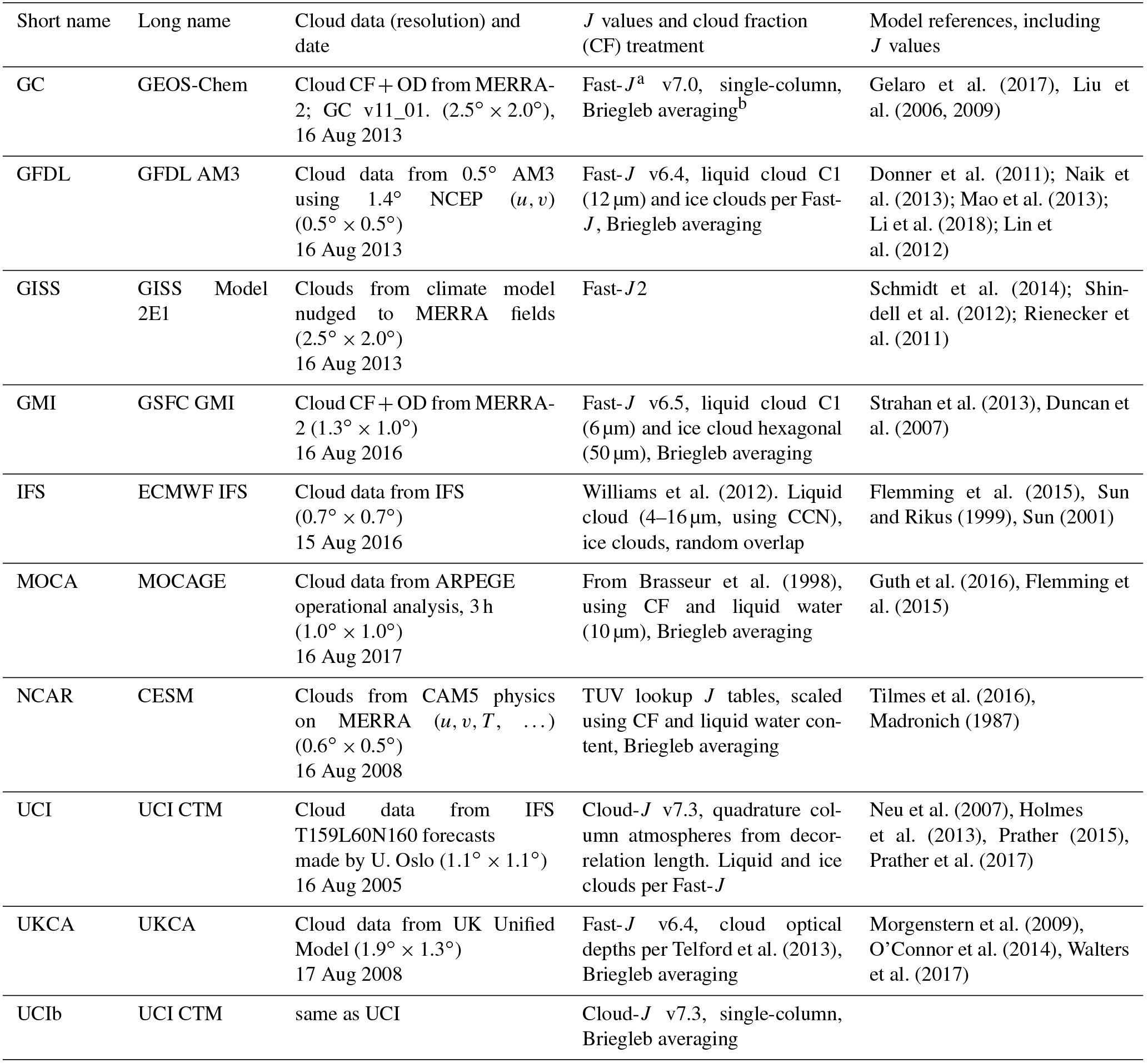
Cloud data include cloud fraction (CF), in-cloud ice/liquid water path and effective radius, or in-cloud ice/liquid optical depth (OD in the visible). a Fast-J versions here are based on Bian and Prather (2002) with updates, including standard tables for cloud optical properties and simplified estimate of effective radius. Cloud C1 refers to Deirmendjian liquid cloud size distribution from the Fast-J data tables (Wild et al., 2000). b Briegleb's method (1992) approximates maximum-random overlap with a single-column atmosphere and adjusted effective cloud fraction such that the cloud optical depth in the grid cell is COD(in-cell) = COD(in-cloud) × CF3∕2.
The models here include the six original ones used in the ATom reactivity studies (Prather et al., 2017) plus three additional European global chemistry models. They are described more fully in Table 1, and are briefly designated as GEOS-Chem (GC), GFDL AM3 (GFDL), GISS Model 2E1 (GISS), GSFC GMI (GMI), ECMWF IFS (IFS), MOCAGE (MOCA), CESM (NCAR), UCI CTM (UCI), and UM-UKCA (UKCA). Additional model information and contacts are given in the Supplement Table S1. All models submitted global 4-D fields (latitude by longitude by pressure for 24 h) for a day in mid-August using their standard treatment of clouds (designated all sky or cloudy here) and then a parallel simulation with clouds and aerosols removed (designated clear sky or clear). In addition to its correlated cloud-overlap model with multiple quadrature column atmospheres to calculate an average J value, UCI also contributed a model version using the B-averaging of cloud fractions (CFs) (Briegleb, 1992) used by most models, designated UCIb (see Prather, 2015). Several models ran the clear-sky case without clouds but with their background aerosols. Globally, aerosols have a notable impact on photolysis and chemistry (Bian et al., 2003; Martin et al., 2003), but over the middle of the Pacific Ocean (this analysis), the UCI model with and without aerosols shows mean differences of order %.
Modeling the effect of clouds on J values began with early tropospheric chemistry modeling. One approach was to perform a more accurate calculation of generic cloud layers off-line and then apply correction factors to the clear-sky Js computed in-line: e.g., an increase above the cloud deck and a decrease below (Chang et al., 1987). Another approach used a climatology of overlapping cloud decks to define a set of opaque, fully reflecting surfaces at different levels; e.g., the Js would be averaged over these sub-grid column atmospheres (Logan et al., 1981; Spivakovsky et al., 2000). As 3-D tropospheric chemistry models appeared, the need for computationally efficient J-value codes led to some models ignoring clouds and others estimating cloud layers and applying correction factors to clear-sky Js. With the release of Fast-J (Wild et al., 2000), some 3-D models started using a J-value code that directly simulated cloud and aerosol scattering properties with few approximations. The next complexity, based on general circulation modeling, included fractional cloud cover within a grid cell and thus partial overlap of clouds in each column (Morcrette and Fouquart, 1986; Briegleb, 1992; Hogan and Illingworth, 2000). This approach later moved on to chemistry models (Feng et al., 2004; Liu et al., 2006; Neu et al., 2007). Monte Carlo solutions for the numerous independent column atmospheres generated by cloud overlap were developed for solar heating (MCICA; Pincus et al., 2003), but random, irreproducible noise was not acceptable in deterministic chemistry transport models. The Cloud-J approach (Prather, 2015) developed a scale-independent 1-D method for cloud overlap based on vertical decorrelation lengths (Barker, 2008a, b). The chemistry models here use a variety of these methods, which range from lookup tables with correction factors, to Fast-J single column, to cloud overlap treatments with Cloud-J; see Table 1. Currently these models do not attempt to define 3-D cloud structures within a grid square, the approach needed to match individual CAFS Js.

Figure 1Profiles of all-sky (cloudy) J-O1D and J-NO2 for the tropical and North Pacific blocks. See Figs. S2 and S3. The CAFS values are directly measured in ATom-1. The 10 models are sampled over 24 h from a day in mid-August, selecting for cos(SZA) > 0.8. The UCI and UCIb models are distinct here because they treat overlapping clouds differently (cloud quadrature vs. B-averaged cloud).
The CAFS data were collected from ATom-1 during its 10 research flights from 29 July to 23 August 2016. It was not possible for the models to simulate each flight path, including clouds and local solar zenith angles (SZAs) for each measurement. Not all of the models could run with 2016 meteorology, and thus we asked for a day in mid-August and treat that (rightly or wrongly) as typical of the cloud statistics during ATom-1. The meteorological dates are listed in Table 1. This simplification made it possible to attract large participation, but of course it limits the ability to claim that the model statistics are a robust climatology. ATom flights are mostly in daylight and hence a large proportion of CAFS measurements occur at high sun, cos(SZA) > 0.6, with more than half at cos(SZA) > 0.8 (Supplement Fig. S1). The models report hourly J-O1D and J-NO2 globally over 24 h, and thus all have a similar distribution of cos(SZA) but with a greater proportion at cos(SZA) < 0.4 than the CAFS data. We restrict these comparisons to high sun, cos(SZA) > 0.8, to reduce 3-D effects that are not modeled here, which leaves 11 504 (block 1) and 4867 (block 2) measurements for the CAFS ∕ TUV 3 s averages. For the models, the number of hourly samples with cos(SZA) > 0.8 is about 18 % for both blocks and thus the number of samples depends on model resolution (e.g., 240 000 for UCI and 1 400 000 for NCAR in block 1). Although the analysis here is limited to the Pacific blocks, the global model data are archived with this paper.
A quick look at J-cloudy (all sky) profiles of J-O1D and J-NO2 for CAFS (Fig. S2) shows a basic pattern also seen in models. Both Js are larger in the upper troposphere where the direct sunlight is more intense, but in the North Pacific, larger cloud cover and more scattered light almost reverses this pattern with enhanced Js at lower altitudes (> 600 hPa). Comparing the variances of J-cloudy (CAFS) and J-clear (TUV) for the tropical Pacific, the J-NO2 variability is driven almost entirely by clouds as expected, while the J-O1D variability is driven firstly by O3 column and sun angle (both CAFS and TUV), while there are clearly cloud contributions (CAFS only) at lower altitudes (> 700 hPa).
Figure 1 shows a full comparison of the CAFS J profiles with the 10 model results in four panels (2 Js × 2 geographic blocks). The CAFS Js fit within the range of models; their shape is matched by most models, but the model spread of order 20–30 % is hardly encouraging. Differences in these average profiles can have many causes: temperature and O3 profiles, spectral data for both J-O1D and J-NO2, ways of integrating over wavelength, surface albedo conditions, treatment of Rayleigh scattering, basic radiative transfer methods, SZA, and, of course, clouds. In typical comparisons we try to control these differences by specifying as many conditions as possible, but here we want to compare the “natural” Js used in their full-scale simulations (e.g., Lamarque et al., 2013) and thus leave each model to its native atmospheres, spectral data, algorithms, and approximations.
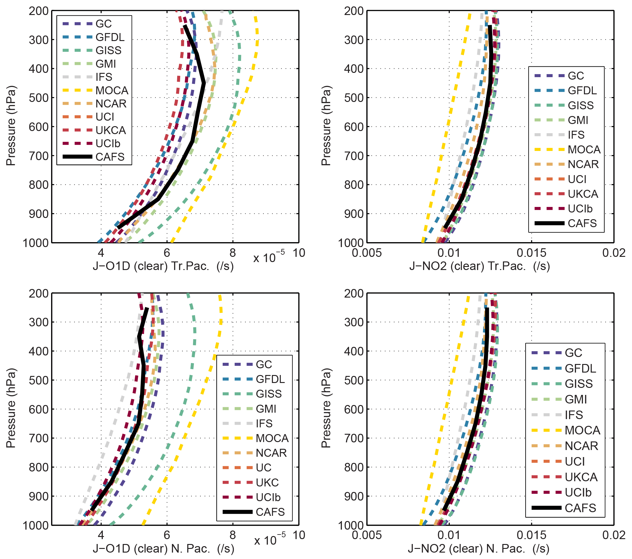
Figure 2Profiles of clear-sky J-O1D and J-NO2 for the tropical and North Pacific blocks. See Fig. 1. CAFS here refers to TUV Js modeled at each point along the flight path. The UCI and UCIb models are not separable since both have the same clear-sky Js. The spread in J-NO2 is likely due to different choices for interpolating cross sections and quantum yields. The J-O1D spread may be caused by the different ozone columns in the Tropics; see Fig. S3.
The models show a much tighter match in J profiles under clear-sky conditions (Fig. 2). Typically, eight of the models fall within 10 % of their collective mean profile. Some models are obviously different in J-clear (GISS and MOCA for J-O1D, MOCA for J-NO2), and these differences carry through to J-cloudy (Fig. 1). A most important factor in J-O1D is the O3 column, and Fig. S3 shows the modeled O3 columns for August compared with 8 years of OMI observations. MOCA, NCAR, and IFS have low tropical O3 columns, < 250 DU vs. observed ∼265 DU, which could lead to higher J-O1D, but this effect is seen only in MOCA. UKCA has higher tropical columns, > 300 DU, which might explain why their J-O1D lies in the lower range of the models. Some results, like MOCA's J-NO2 and GISS's J-O1D point to differences in the implementation of spectral data (e.g., wavelength integration, solar spectrum, temperature interpolation). We expect GC and GMI to be alike since they both use MERRA-2 cloud fields and Fast-J with Briegleb averaging: indeed, they match well except for J-O1D in the tropical Pacific, yet, they report similar tropical ozone columns.
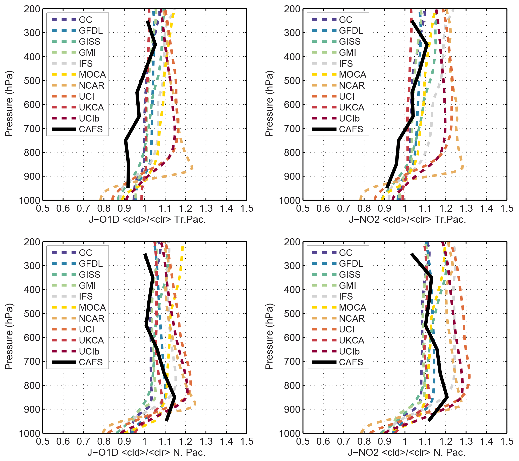
Figure 3Profiles of the ratio of the average of J-cloudy to the average of J-clear for J-O1D and J-NO2 and for the two Pacific blocks. See Figs. 1 and 2.
The ratio of J-cloudy to J-clear, shown in Fig. 3, cancels out many of the model differences in Figs. 1 and 2, and as expected GC and GMI are nearly identical. The cloudy : clear ratio identifies new patterns in model differences, whereby some models have ratios close to 1 throughout the troposphere (especially in the Tropics) while others have ratios > 1.1 at altitudes above 800 hPa and < 0.9 below 900 hPa. In a recent model intercomparison with specified chemical abundances (Prather et al., 2018), we found that the tropospheric photochemistry of O3 and CH4 responded almost linearly to cloudy–clear changes in J values (see Fig. S4; data not shown in Prather et al., 2018). Thus the differing impact of clouds on J values seen in Fig. 3 will have a correspondingly large impact on global tropospheric chemistry (see Liu et al., 2009).
The average ratio of J-cloudy to J-clear (Fig. 3) provides only a single measure of the impact of clouds. The CAFS data provide a more acute measure by sampling the range of cloud effects (enhance or diminish J values) and their frequency of occurrence. A quick look at this range in CAFS data is shown in Fig. S5 with the probability of occurrence of the cloudy : clear ratio defined as ln(J-cloudy/J-clear) and designated rlnJ. Each curve is normalized to unit area, with the y axis being probability per 0.01 bin (∼1 %) in rlnJ.
We expect that enhancements in Js occur above clouds and diminishments below, and this is shown in Fig. S5. In the marine boundary layer (900 hPa–surface), there are a greater number of rlnJ < −0.10, with fewer rlnJ > 0.00. In the mid-troposphere layer (300–900 hPa), there are frequent occurrences of rlnJ > +0.10, particularly in the North Pacific where lower level clouds are more extensive than in the Tropics. Likewise, there are times when rlnJ is < 0.00 in the mid-troposphere when clouds lie overhead. In upper tropospheric layers (100–300 hPa), most of the optically thick clouds are below and rlnJ > 0.00 is dominant. Thus, our analysis here breaks the atmosphere into these three layers. All figures in this section will be displayed as two-block by three-layer panels with part a (J-O1D) and part b (J-NO2).
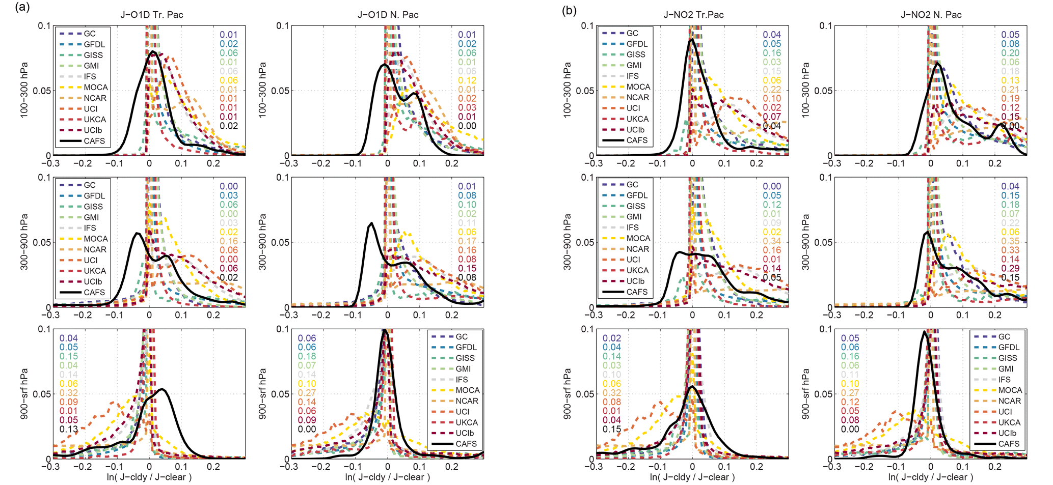
Figure 4(a) Probability distribution of the natural log of the ratio of cloudy–clear J-O1D values (rlnJ) from 10 models and from CAFS during ATom-1. The columns correspond to the two geographic blocks (tropical Pacific, 20∘ S–20∘ N × 160–240∘ E, and North Pacific, 20–50∘ N × 170–225∘ E). The rows are the three pressure layers (100–300, 300–900, 900–surface hPa). All histograms sum to 1, but for many models the peak values about rlnJ = 0, corresponding to cloud-free skies, are truncated. Where a significant fraction of events does not fit within the ±0.3 range – on the high side for 100–900 hPa and low side for 900–surface hPa – the column of numbers, placed on the appropriate side and color coded to the legend, gives the fraction of occurrences outside the range. (b) Probability distribution of the natural log of the ratio of cloudy–clear J-NO2 values (rlnJ) from 10 models and from CAFS during ATom-1. In general, J-NO2 is more responsive to clouds than J-O1D is.
3.1 Modeling the distribution of J values
The probability distribution of rlnJ for J-O1D (Fig. 4a) and J-NO2 (Fig. 4b) shows highly varied patterns across the models, but with some consistency. The models and CAFS are not exactly a match, but again, there are some encouraging patterns. The peak rlnJ distributions for CAFS will be broadened because the real variation in ocean surface albedo is not simulated in TUV (see discussion in Sect. 4), but this is expected to be of order ±2 %, and so the overall width (10 to 20 %) reflects cloud variability. The modeled and measured distributions are asymmetric and skewed toward rlnJ > 0 in the free troposphere (100–900 hPa), and toward rlnJ < 0 in the boundary layer. This pattern is expected since Js are enhanced above clouds (100–900 hPa) and diminished below. There will also be some occurrences of rlnJ < 0 in the free troposphere when thick clouds are overhead, but none of the models come close to the CAFS frequency of these occurrences. In general and as expected, this brightening above and dimming below is more evident for J-NO2 than for J-O1D. Another feature that is somewhat consistent across models and observations is that the wings of the rlnJ distribution are wider in the North Pacific than the Tropics. In the boundary layer, observations and models show the reverse with greater cloud effects (dimming, rlnJ < 0) in the Tropics. Although all the models show this shift from rlnJ > 0 to rlnJ < 0 in the peak of their distributions, only a few (GISS, MOCA, NCAR, UCI) have broad wings of large cloud shielding (rlnJ < −0.1). These models calculate such broad wings for both the Tropics and North Pacific, whereas CAFS only shows this in the Tropics.
These diagnostics also identify some CAFS anomalies that have no physical basis in the current models. For example, low-level (surface to 900 hPa) observed cloud enhancements (rlnJ > 0.025) observed in the tropical Pacific (particularly J-O1D) do not appear in the models. Similarly cloud diminishments in the upper troposphere do not appear with the modeled cirrus. A more thorough analysis of the CAFS rlnJ with the added deployments should examine if these differences are due to 3-D radiative transfer effects, ocean albedo variations, or missing cloud types in the models. Perhaps, we will identify sun–cloud geometry conditions simply not possible in the 1-D cloud models.
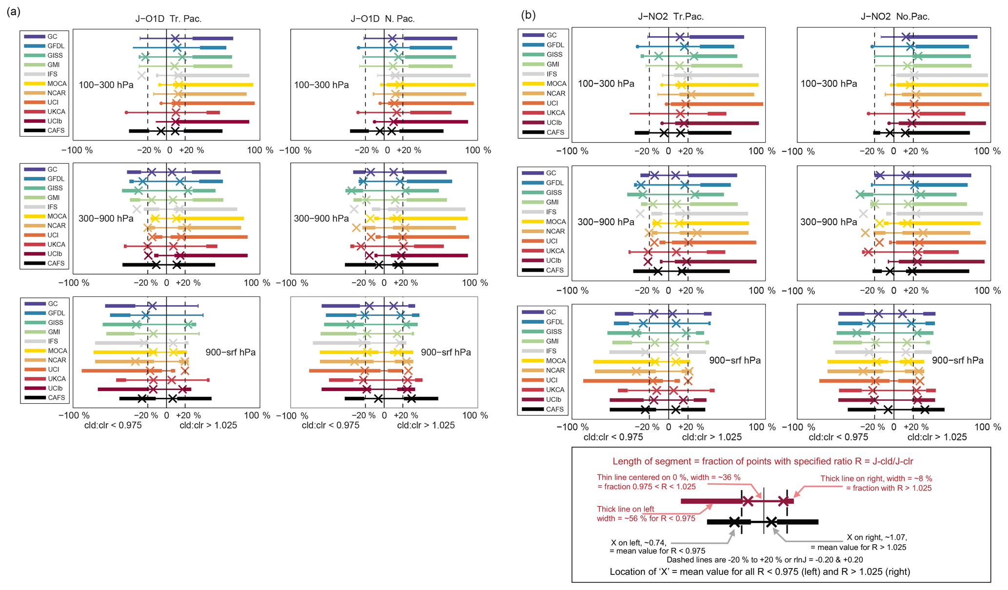
Figure 5(a) Frequency of occurrence and magnitude of change in J-O1D caused by clouds. The panels and data sources are the same as in Fig. 4ab. The horizontal lines all have length 1 and show the fraction of (i) cloud-diminished Js (thick left segment, cloudy : clear ratio < 0.975), (ii) nearly cloud-free Js (thin central segment, 0.975 < ratio < 1.025), and (iii) cloud-enhanced Js (thick right segment, ratio > 1.025). Each line is plotted with its nearly cloud-free segment centered on 0. The mean magnitude of diminishment/enhancement corresponding to the thick line segments is plotted as an “X” on each line segment, using the x axis [−1, +1] as the natural log of the cloudy : clear ratio. Ratio changes of −20 % and +20 % are shown as dashed vertical grid lines. The Xs are not shown when the frequency of occurrence of either thick segment is < 0.02. For an example of how to read these figures consider the panel in row 3 column 1 (J-O1D, Tr. Pac, 900–srf). The GFDL model has about 22 % cloud-diminished Js (left segment) with an average value of 22 % below clear-sky Js (the X on the left side); most of the remaining, 76 %, are nearly cloud-free (central thin segment). The GISS model has (from left to right) 42 % cloud-diminished Js, 53 % cloud-free Js, and only 5 % cloud-enhanced Js for a total of 100 %; the cloud-diminished Js average about 28 % less than clear-sky Js (the X on the left) while the cloud-enhanced Js average about 22 % greater (the X on the right side). See legend in Fig. 5b. (b) Frequency of occurrence and magnitude of change caused by clouds in J-NO2.
Figure 5a (J-O1D) and b (J-NO2) provide another view of the rlnJ statistics. Figure 5 has the same six blocks as Fig. 4, but plots five quantities schematically in a single line describing each model's statistics: percent occurrence of diminishment (rlnJ < −0.025), average rlnJ diminishment, percent occurrence of nearly clear sky, percent occurrence of enhancement (rlnJ > +0.025), and average rlnJ enhancement. The horizontal line has a total length of 100 % with the thin line (clear sky) centered on 0; see the extended legend in Fig. 5b.
Overall, four models (GC, GFDL, GMI, UKCA) have unusually narrow peak distributions of rlnJ ∼0, indicating lesser cloud effects on the Js. The other six models (GISS, IFS, MOCA, NCAR, UCI, UCIb) show a much greater range in Js, with a larger fraction perturbed by clouds (enhanced or diminished by more than 10 %). The CAFS observations generally support this latter group. There are individual model anomalies that may point to unusual features: MOCA alone has a peak frequency of enhanced Js at rlnJ ∼0.05 in the free troposphere; three models (NCAR, UCI, UCIb) show the largest extended frequency of |rlnJ| > 0.10 in the middle troposphere; UKCA is consistently the most clear-sky model. These model differences are not simply related to the model cloud fields; see discussion of Fig. S6 below.
Immediately above and below extensive thick cloud decks the dimming/brightening of Js exceeds the plotted range of rlnJ of ±0.3 (a factor of 1.35). Most such cloud decks occur around 900 hPa and so the largest brightening occurs in the 100–900 hPa levels, and the greatest dimming at > 900 hPa. The top two rows in Fig. 4 give the fraction of samples for which rlnJ > 0.3 on the right side of each plot; the bottom row gives, on the left side, the fraction for which rlnJ < −0.3. The categorization of models and measurements is not simple as many models have shifting magnitudes of this large-scale brightening or dimming. A few models consistently lack these large changes in Js (GC, GMI), and a few always have them (NCAR, UCIb). Large CAFS values are clearly evident in both Js for only two of the six cases: > 900 hPa in the tropical Pacific (13–15 % of all Js) and 300–900 hPa in the North Pacific (8–15 %). For these cases the CAFS extreme fractions are consistent with at least four of the models. Any possible CAFS bias in rlnJ due to TUV modeling (±0.05) is unlikely to affect these results. These extreme fractions, however, are likely sensitive to any sampling bias of flight path with respect to thick cloud decks, and this needs to be assessed with model sampling that matches the ATom-1 profiles of that period.
The large geographic blocks were chosen to acquire representative sampling from the models that would be repeatable over time. It was not possible to acquire month-long or multi-year diagnostics from all the models, and so with the available model results (24 h from a day in mid-August) we subsample the broad tropical Pacific block (20∘ S–20∘ N × 160–240∘ E) into a west (160–200∘ E), east (200–240∘ E), and dateline (175–185∘ E) block. The results of these subsampled statistics are shown for J-NO2 in Fig. S7a (100–300 hPa) and b (surface–900 hPa) using the same format as Fig. 5. Each of the 18 panels in Fig. 7a, b represents a single model and a single pressure level for which there are seven bars (sampled distributions of rlnJ). The top four bars show the full tropical Pacific (as in Fig. 5b) and then the three subsampled regions. The next three bars are the previously sampled statistics (North Pacific, global 50∘ S–50∘ N, and tropical Pacific CAFS). The CAFS bars are the same in each nine-panel plot. Six models show no difference across the subsampling (NCAR, GFDL, IFS, UCI, UKCA, MOCA), while three models using MERRA cloud fields in one way or another (GC, GMI, GISS) show weaker cloud effects in the east half of the region. For the most part, the subsampled regions have similar statistics that are distinct from the CAFS observations. Thus our model statistics over a large block may be a representative climatology of cloud effects on J values. Further sampling tests are recommended for follow-on work, especially to determine if the distinct east–west differences for the three MERRA cloud models are a standard feature.
3.2 Analyzing cloud effects
With a graphical synopsis of the rlnJ probability distributions in Fig. 5a, b, some model features become more obvious. We define nearly cloud-free conditions as being within ±2.5 % of clear-sky Js, and show the frequency of these with the length of the thin line in the center of the plots. Starting with the J-O1D in the upper tropical Pacific, we find five models (Group 1: GC, GFDL, GMI, GISS, UKCA) show no effect of clouds more than 50 % of the time. The other 40–50 % of the time, they show enhanced J-O1D, cloud brightening expected from clouds below (thick lines on the right side of the plot). For the other five models (Group 2: IFS, MOCA, NCAR, UCI, UCIb), these clear-sky equivalent Js occur only 10–20 % of the time, with cloud brightening enhancements occurring at 80–90 %. Surprisingly, both model groups show the same average magnitude, +10 % (Xs on the right side), for their enhanced Js. Thus Group 2 models will have systematically greater J-O1D in the upper tropical Pacific than the Group 1 models (i.e., the 10 % enhancement occurs twice as often). In the North Pacific, this pattern holds although both groups show slightly greater frequency of enhanced Js, e.g., 50 to 60 % for Group 1 and 80 to 90 % for Group 2. For J-NO2, the results are similar, but with greater average magnitude of enhancement for cloudy skies (20 % vs. 10 %) and a slightly greater frequency of occurrence (thick line on the right). For this upper tropospheric layer, none of the models show significant occurrence of diminished J values from overhead clouds (rlnJ < −0.025) as seen in CAFS for 2–12 % of the measurements.
In the middle troposphere (300–900 hPa, middle panels), the patterns in clear-sky frequency remain unchanged, but there is a shift to cloud dimming for 5 to 20 % of the time. This shift to more cloud obscuration is much greater in CAFS than in any model. Group 1 models show consistently more frequent cloud obscuration (10–20 %) than Group 2 models do (5–10 %). When cloud brightening occurs (both CAFS and models), the magnitude of enhancement is greater than in the upper troposphere. Such a pattern is consistent with the simple physics that Js are greater immediately above a cloud than high above it.
In the boundary layer, most clouds are above, and cloud obscuration leads to increased occurrence of rlnJ < −0.025 compared to the middle troposphere (in both CAFS and models). Even though the frequency changes, the average magnitude of diminishment when there is cloud obscuration (denoted by Xs) does not change much across models in either region. For CAFS in the tropical Pacific, however, the diminishment when there is cloud obscuration is much larger in the boundary layer. The modeled shifts in frequency of occurrence from enhanced to reduced Js are dramatic, but still the Group 1 pattern of nearly 50 % clear-sky Js persists. This results in Group 2 having a much larger frequency of diminished Js (60–80 %) as compared with Group 1 (20–40 %).
Using CAFS data to define nearly cloud-free conditions is imperfect. Potential biases exist with TUV modeling of J-clear and are related to albedo as discussed in Sect. 4. In addition, the CAFS data do not represent a true climatology due to flight planning and flight operations that tend to avoid strong convective features and thick cloud decks, particularly near the surface. Such biases can shift the distribution as well as widen it through noise, and this may explain some of the increased width of the CAFS peak and the 1 to 2 % offsets of the clear-sky peaks in Fig. 4. It is difficult to select between Group 1 and 2 using CAFS. The CAFS clear-sky fraction lies between that of the two groups in the upper troposphere but becomes narrower in the boundary layers, more closely matching that of Group 2. Given that a number of processes can lead to broadening of the CAFS distribution, it is likely the sharps peaks in Fig. 4 (and wide central lines in Fig. 5) of Group 1 are unrealistic.
These model differences have no obvious, single cause. The modeled profiles of COD and CF for both geographic blocks are shown in Fig. S6 (note the logarithmic scale for COD). The total COD is given (color coded) in each block. The profiles show very large variability that is hard to understand. For example, GFDL and GISS show the largest COD, yet both are in Group 1 with the largest fraction of clear sky. Overall the total COD does not obviously correlate with the two groups. Likewise, CF is not a predictor for the group. It is likely that model differences are driven by the treatment of fractional cloud cover. For example, GMI (Group 1) and UCI (Group 2) have very similar CODs and CFs in the lower troposphere as shown in Fig. S6. They also use similar J-value codes including spectral and scattering data based on the Fast-J module. Yet, they have a factor of 2 difference in the frequency of nearly cloud-free sky as shown in Fig. 5. Compared to GMI, UCI shows an overall greater impact of clouds with 2 times larger frequency of cloud brightening in the upper troposphere and 2 times larger occurrence of cloud dimming in the boundary layer. These differences could be caused by GMI calculating J values with a single-column atmosphere (SCA) containing clouds with Briegleb (CF3∕2) averaging and UCI calculating J values with four quadrature column atmospheres (QCAs); see Table 1. Unfortunately, when UCI mimics the B-averaging (with model UCIb), the differences remain. See further discussion of Fig. S6 in Sect. 4.1.
The J-value statistics here depend on (i) the cloud fields used in the models, (ii) the treatment of cloud overlap statistics, (iii) the radiative transfer methods used, and (iv) the spectral data on sunlight and molecular cross sections. These components are deeply interwoven in each model, and it is nearly impossible to have the models adopt different components except for (iv), for which there has been a long-standing effort at standardization (e.g., the regular IUPAC and JPL reviews of chemical kinetics; Atkinson et al., 2004; Burkholder et al., 2015). These components are briefly noted in Table 1.
4.1 Cloud optical depths and overlap statistics
The models reported their average in-cell cloud optical depth (per 100 hPa) and cloud fraction over the two Pacific blocks in Fig. S6. Averaged cloud optical depths (defined for the visible region 500–600 nm) all tend to peak below 850 hPa in the Tropics and decline with altitude. There is clear evidence of mid-level (400–800 hPa) clouds, but only small COD (total < 0.25) at cruise altitudes (100–300 hPa). The North Pacific block has 2–4 times larger low-altitude COD. The plotted CF is the COD-weighted average over 24 h and all grid cells in the block. Note that for COD the cloud is spread over each model layer, and hence the in-cloud optical depth is estimated by COD/CF. CF is high, 5–15 % below 850 hPa, drops off with altitude as does COD, but peaks at 10–20 % near 200 hPa corresponding to large-scale cirrus. Some of these differences in COD and CF are large enough to explain model differences, but there is no clear pattern between J values and clouds as noted in Sect. 3.2. A more thorough analysis and comparison of the modeled cloud structures would involve the full climate models and satellite data (Li et al., 2015; Tsushima et al., 2017; Williams and Bodas-Salcedo, 2017), beyond the scope here.
4.2 Sensitivity of rlnJ to small cloud optical depth
To relate total COD to a shift in rlnJ, the UCI off-line photolysis module Cloud-J was run for marine stratus (CF =1) with a range of total CODs from 0.01 to 100. The cloud was located at about 900 hPa and rlnJ evaluated at 300 hPa. The plot of rlnJ vs. log COD for a range of SZAs is shown in Fig. S8. A 10 % enhancement (rlnJ ) occurs at COD =5 for J-O1D and COD =3 for J-NO2, demonstrating the greater sensitivity of J-NO2 to clouds. Thus model average total COD (ranging from 0.8 to 11 in Fig. S6, assuming CF =1) should produce large shifts in rlnJ. Marine stratus with typical COD ∼10 or more would produce rlnJ-O1D of +0.16 and rlnJ-NO2 of +0.30. Thus clear-sky J values (defined here as ±0.025 in rlnJ) require COD < 1 for J-O1D and < 0.3 for J-NO2. A COD ∼1 is not that large since these clouds are highly forward scattering and have an isotropic-equivalent optical depth that is 5 times smaller.
4.3 Averaging over clouds affects clear-sky fraction
Comparison of the CAFS-ATom measurements of J values with modeled ones presents a fundamental disconnect, but one that we must work through if we are to test the J values in our chemistry–climate models with measurements. A CAFS observation represents a single point with unique solar zenith and azimuth angles within a unique 3-D distribution of clouds and surface albedos. Ozone column and temperature also control J values but are less discontinuous across flight path and model grids. One can define a column atmosphere (CA) for each J value in terms of the clouds directly above/below and the surface albedo, as would be measured by satellite nadir observations. The CAFS-measured actinic flux includes direct and diffuse light, which depends on all the neighboring CAs out to tens of kilometers. Adjacent clouds can either increase or decrease the scattered sunlight at the measurement site depending on the location of the sun.
By including cloud fractional coverage from the meteorological models, and attempting in various ways to describe cloud overlap, the models here recognize that the atmosphere is not horizontally homogeneous. Yet, for cost effectiveness and non-random J values, most modeling solves the radiative transfer problem for a 1-D plane-parallel atmosphere that is horizontally homogeneous. Most chemistry models adopt a simple averaging procedure to create a single, horizontally homogeneous cloudy atmosphere in each grid cell and then solving for a single J value (see Table 1). The UCI model uses decorrelation lengths to determine cloud overlap, to generate a set of independent column atmospheres (ICAs), to generate four quadrature column atmospheres (QCAs), and to calculate four J values, which are then averaged to get a single J value. In either case, the radiative transfer solution is 1-D and there is one J value per grid cell given to the chemistry module (and analyzed here).
What would the probability distribution rlnJ look like if we used the UCI J values from the QCAs before averaging? For this, we collect the statistics on total COD for the two geographic blocks and compare the sub-grid QCA CODs against averaging approaches in Fig. 6. This histogram (blue dots) is our best estimate of the distribution of total COD from a 1-D nadir perspective of all the sub-grid ICAs. The UCI J values are calculated as the average over four QCAs as representatives of the ICAs. The two SCA models use simple averaging (COD × CF, green dots) and B-averaging (COD × CF3∕2, orange dots), which reduces the cloud fraction but assumes maximal cloud overlap. In these cases, a single J-value calculation is made with the SCA. When the clouds are simply averaged over the grid cell (), the clear-sky occurrence drops to 7 % and the deep cumulus disappears. When Briegleb (1992) B-averaging is used, there is only slightly more clear sky (12 %). Both averaging methods also reduce the occurrence of thick cumulus. When run at lower resolution, both averages find less clear sky, while the QCA statistics are not affected by resolution in the range 50–200 km. This averaging, of either J values or clouds, explains why most models do not produce a single, sharp peak at rlnJ =0.
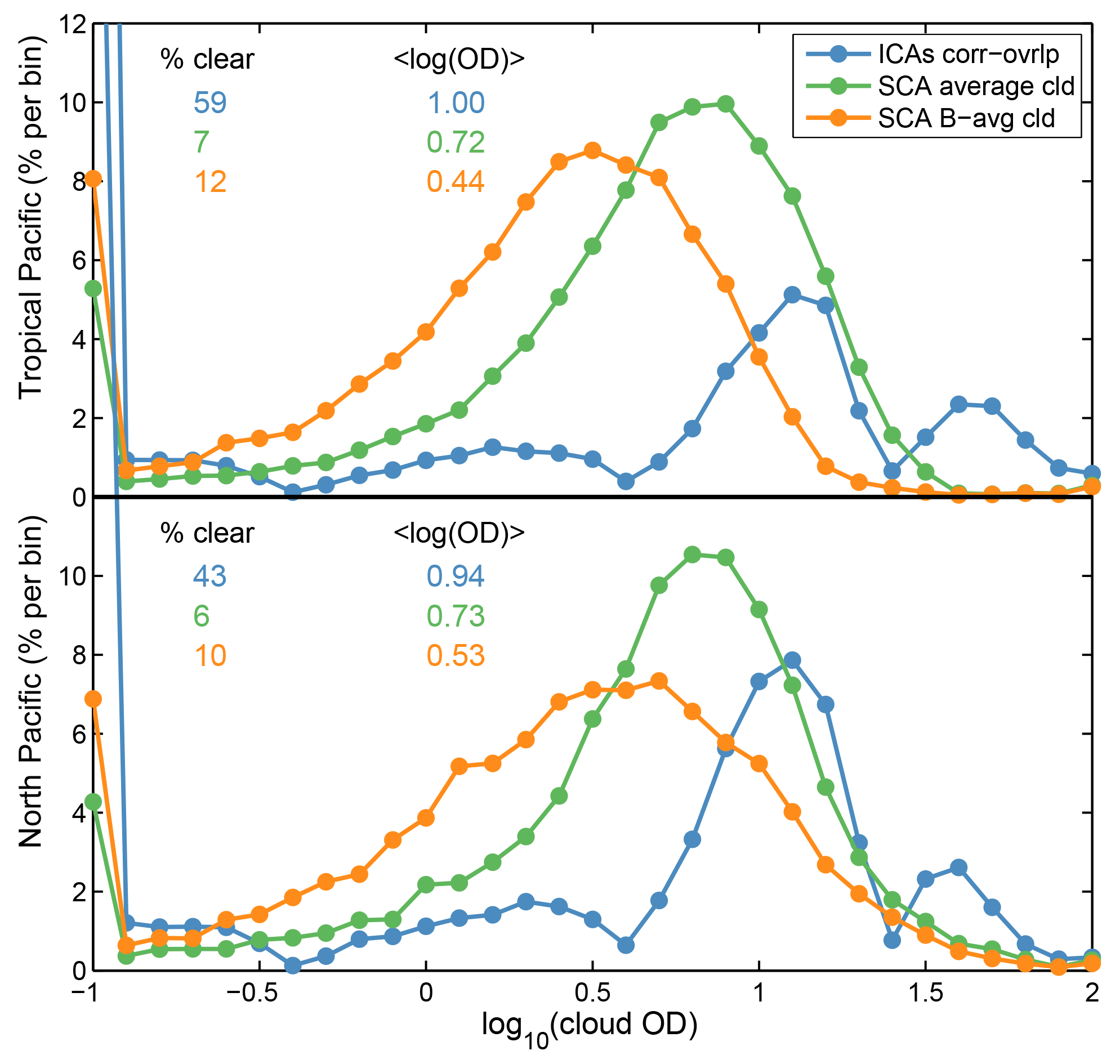
Figure 6Histogram (% per 0.1 bin) in log of the total cloud optical depth (COD) based on method of implementing fractional clouds: Cloud-J independent column atmospheres (ICAs, blue dots); simple cloud averaging over each cell (COD × CF, green dots) and B-averaging (COD × CF3∕2, orange dots). The 600 nm COD for two large regions (tropical Pacific, 20∘ S–20∘ N × 160–240∘ E, and North Pacific, 20–50∘ N × 170–225∘ E. is collected for 16 August 2016 from eight 3 h averages of COD and cloud fraction (CF) in each model layer. The “% clear” is the sum of fractions (%) with log10(total COD) < −0.5; and the “< log(OD)>” is the average of log10(total COD) > −0.5. The cloud fields come from the ECMWF IFS cycle 38 system run at T159L60N160 resolution. On average the number of ICAs per cell in the tropical block is about 170, although individual cells may have > 1000. In spite of the high, 40–60 % fraction of clear columns, the quadrature-averaged J values usually include some cloudy fraction.
At sufficiently high model resolution, where CF is either 0 or 1, a new problem arises because the radiative transfer problem is now clearly 3-D. The 1-D radiative transfer used here would produce a very sharp clear-sky peak in rlnJ that is not seen in CAFS. The CAFS rlnJ distribution is widened in part by TUV albedo biases, but also because it is effectively a weighted average of cloud conditions over tens of kilometers or more and thus has lower frequency of clear sky than the 1-D ICAs do. The Group 1 models with large peak distributions at rlnJ ∼0 appear to be basically incorrect since averages over these model resolutions (> 0.5∘) should reduce clear-sky occurrence. There is probably a sweet spot in model resolution at about 20 km where the model statistics, even with 1-D RT, should match the observed statistics.
4.4 Ocean surface albedo
We chose our Pacific blocks for this comparison to avoid large aerosol contributions and to be oceanic to avoid large variations in surface albedo. Nevertheless, the ocean surface albedo (OSA) is variable (Jin et al., 2011), but most of these models, including TUV, assume a uniform low albedo in the range of 0.05 to 0.10. For the modeled ratio J-cloudy to J-clear, using a fixed albedo is not so important since both J values use the same albedo. For the CAFS ∕ TUV ratio, however, it is essential to have the TUV model use the OSA that best corresponds to the sea surface conditions under the CAFS measurement. Work on the CAFS ∕ TUV calibration seeks to achieve this zero bias, and it continues beyond the cutoff date of the ATom-1 data used here. The OSA affects our 2 Js differently: for J-O1D with peak photolysis about 305 nm, the OSA under typical conditions (SZA = 20∘, surface wind = 10 m s−1, chlorophyll = 0.05 mg m−3) is 0.038, while for J-NO2 with peak photolysis at 380 nm, the OSA is 0.048. OSA depends critically on the incident angle of radiation, increasing from 0.048 at 20∘ to 0.068 at 50∘ (380 nm). Rayleigh scattered light has on average larger incident angles than the solar beam for CAFS measurements and is reflected more than the direct beam. Rayleigh scattering is much more important for J-O1D than J-NO2.
The UCI stand-alone photolysis model was rewritten to include a lower boundary albedo that varies with angle of incident radiation, and is now designated Cloud-J version 8 (v8). In Cloud-J there are five incident angles on the lower surface: the direct solar beam and the four fixed-angle downward streams of scattered light. The OSA modules are adapted from the codes of Séférian et al. (2018) based on Jin et al. (2011), but we do not use their approximation for a single “diffuse” radiation since all of Cloud-Js scattered light is resolved by zenith angle. The resulting albedo is a function of wavelength, wind speed, and chlorophyll; it is computed for each SZA and the four fixed scattering angles. As a test of the importance of using a more realistic OSA, we used Cloud-J v8 to compute the ratio of J with our OSA module to J using a constant fixed albedo, with both Js calculated for clear sky. We calculate this rlnJ (log of the ratio of J-clear (OSA) to J-clear (single albedo)) for a range of SZAs, wind speeds, and chlorophyll comparing to fixed albedos of 0.00, 0.06, and 0.10 as shown in Fig. S9. Because of the range in conditions, there is no single offset, but we have a probability distribution whose width in rlnJ due to a range of surface albedo has a magnitude that affects the interpretation of measurement–model differences. For high sun (SZA = 0–40∘), choosing an optimal fixed albedo of 0.06 results in little mean bias, although individual errors are about ±2 %. This error is based on conditions for cos(SZA) > 0.8. If the fixed albedo differs from this optimum (e.g., 0.00 or 0.10), then bias errors of 2 % to 10 % appear, and the width of the distribution expands greatly. For SZA = 40–80∘, the optimum fixed albedo starts showing bias and has a much broader range of errors under different circumstances (wind, chlorophyll, SZA). Thus J values calculated using unphysical, simplistic fixed ocean surface albedos can have errors of order ±10 % depending on ocean surface conditions and the angular distribution of direct and scattered light at the surface. These errors will not directly affect the model results here since the cloudy–clear differences used a self-consistent albedo in each model. Overall, however, there is a need for chemistry models to implement a more physically realistic OSA.
The importance of clouds in altering photolysis rates (Js) and thence tropospheric chemistry is undisputed. On a case level it is readily observed, and on a global level, every model that has included cloud scattering finds significant changes in chemical rates and budgets. For example, the inclusion of cloud layers by Spivakovsky et al. (2000) caused a shift in peak OH abundance from the boundary layer to just above it, resulting in a shift to colder temperatures (and lower reaction rates) for the oxidation of CH4-like gases, even with the same average OH abundance. Other than single-column, idealized, off-line tests of radiative transfer methods, we have few methods to constrain modeled Js under cloudy conditions.
The impact of clouds on Js is large, simply by looking at the profile of mean Js (Figs. 1, 2, and 3), and it greatly complicates the comparison of J values across models. The modeled mean clear-sky profiles, including the CAFS TUV model (Fig. 2), tend to agree within ±10 % with the exception of MOCA, GISS, and sometimes IFS. However, the all-sky (cloudy) profiles (Fig. 1) have a much wider spread, except for J-O1D in the North Pacific for which there is inexplicably a core group of eight models within ±10 %. The observed CAFS cloudy profiles show a distinctly different profile in the North Pacific vs. the tropical Pacific for both J-O1D and J-NO2 (Fig. 1) and especially in the CAFS ∕ TUV derived J-cloudy to J-clear ratios (Fig. 3). Many models follow this typical profile in the tropical Pacific (100–900 hPa; Fig. 3), but some (NCAR, UCI, UCIb) show large shifts to enhanced J values immediately above the marine boundary layer. Whether this fundamental shift in cloud regimes is robust remains uncertain, and may be resolved with the full set of ATom deployments or with careful model studies; see below.
A more informative diagnostic of cloud effects is the statistical distribution of the individual J-cloudy to J-clear ratios (rlnJ). To model clouds correctly we need to understand how frequently and by how much clouds interfere with J values. The statistical distribution of rlnJ shows distinct patterns and classes of models. In the free troposphere (100–900 hPa), all have a sharp edge at rlnJ =0 with hardly any diminished J values (rlnJ < 0), but the small-cloud-effects models (GC, GFDL, GISS, GMI, UKCA) show a dominant peak at rlnJ ∼0 while the large-cloud-effects models (IFS, MOCA, NCAR, UCI, UCIb) have extensively enhanced J values with large fractions at +25 % or more. In the marine boundary layer (surface–900 hPa), this pattern is reversed with a sharp edge for all models at rlnJ , and the large-cloud-effects models showing more diminished J values. CAFS ∕ TUV has its own pattern, which is very broadened, but generally supports the large-cloud-effect models. If further analysis can tighten the CAFS rlnJ distribution, then we may be able to discriminate among the models in one of the classes. One robust result from the models is that large cloud effects (|rlnJ| > 0.05) are always asymmetric, splitting in sign above and below 900 hPa. If the symmetric spread in CAFS rlnJ remains robust with additional deployments and efforts to reduce CAFS-TUV inconsistencies, then we have a clear challenge for the cloud climatologies used in the chemistry models.
More work on the CAFS ∕ TUV data could help better discriminate among the model classes identified here. For one, we need to sample over different seasons and synoptic conditions to build a more robust climatology. Fortunately, the additional three deployments (ATom-2, -3, -4) will provide these. They occur in different seasons, which is a consideration, but the tropical oceanic data can probably be combined. The analysis can be extended to the Atlantic. CAFS or similar measurements from other aircraft missions could also be added. Other tasks involve tightening the spread in rlnJ by looking for potential measurement–model noise (e.g., aircraft–sun orientation, sun–cloud geometries) and by improving the TUV clear-sky modeling (e.g., a more accurate ocean surface albedo derived from observed surface wind, chlorophyll, SZA). An unresolved issue is how to treat aerosols, both in the models and in CAFS. If clear sky includes aerosols then TUV must be able to infer an aerosol profile for all measurements, and likewise the models need to be careful in how they calculate cloudy–clear ratios. Fortunately for most of the oceanic ATom measurements, aerosol optical depths are small, but where they are large (e.g., Saharan dust events) the daily satellite mapping should provide adequate coverage for the TUV modeling. Developing these cloudy–clear J-value statistics over land will be more difficult due to the higher inherent variability in albedo and aerosol profiles.
More effort is needed from the modeling community to characterize the key factors driving these model differences in photolysis rates under realistic, cloudy conditions. This might include sensitivity runs that address aerosol and surface albedo impacts for each model. We would also need a better characterization of the cloud distributions used in chemistry models, including comparison with satellite climatologies (Cesana and Waliser, 2016; Ham et al., 2017), to understand how cloud fraction and overlap affects the Js used in the photochemical calculation of a column atmosphere. Models can help assess the ATom CAFS statistics for representativeness by checking on flight routing, multiple days, or different years.
The 3-D nature of the radiation field measured by aircraft presents a more fundamental challenge. The observations average over cloud fields out to tens of kilometers, and even if the atmospheric column at the aircraft is clear, neighboring clouds alter J values. The chemical models are coarse resolution compared with the CAFS measurements and average over wider range of cloud fields, almost eliminating the occurrence of clear-sky conditions. Even if they calculate a distribution of J values for the cloud statistics in a column (like Cloud-J), they combine these to deliver a single average J value for the chemistry module, again reducing the occurrence of clear-sky J values. Thus, the result above (i.e., that five models have about 50 % nearly clear-sky J values down to the surface) is inexplicable unless they have column optical depths of 0.3 or very small effective cloud fractions. At some model resolution, probably of order tens of kilometers, the CAFS measurements may be a statistical representation over that grid, and our comparisons, even with 1-D radiative transfer over a range of ICAs, may be more consistent. At these scales, the problem of a strong zenith angle dependence remains (Tompkins and Giuseppe, 2007). Super-high-resolution models (∼1 km) are becoming available in regional or nested-grid models (Kendon et al., 2012; Schwartz, 2014; Berthou et al., 2018), and one might hope that our problem is now solved because each single-column atmosphere (SCA) explicitly resolves cloud overlap, with each grid cell being either cloudy or clear. The calculation of photolysis and solar heating rates is not simplified, however, because now the SCAs interact with neighbors. Calculating the correct rates at any location, or even the average over a region, would require that we calculate the ratio of cloudy to clear over a 20 km domain of cloud-resolved grid cells.
The data sets used here (global hourly J values) for the plots and analysis are extensive (∼10 GB) and will be archived at the Oak Ridge National Laboratory DAAC. This also includes the 3 s CAFS from all ATom-1 research flights. See Hall et al. (2018); https://doi.org/10.3334/ORNLDAAC/1651. The data analysis and plotting codes, as MATLAB scripts, are also archived there.
The supplement related to this article is available online at: https://doi.org/10.5194/acp-18-16809-2018-supplement.
SRH and MJP designed this analysis. MJP developed the codes to analyze, compare, and plot the data. SRH and KU performed the CAFS analysis and contributed those data. All others ran the prescribed model experiments and contributed their model data. MJP and SRH prepared the manuscript with review and edits from all other co-authors.
The authors declare that they have no conflict of interest.
This work is supported by the ATom investigation under the National
Aeronautics and Space Administration's (NASA) Earth Venture program (grants
NNX15AJ23G, NNX15AG57A, NNX15AG58A, NNX15AG71A), Earth Science Project Office
(see https://espo.nasa.gov/atom/content/ATom), and the Oak Ridge
National Laboratory Distributed Active Archive Center (see
https://daac.ornl.gov/ATOM). The National Center for Atmospheric
Research is sponsored by the National Science Foundation. The UKCA
simulations used the NEXCS High Performance Computing facility funded by the
U.K. Natural Environment Research Council and delivered by the Met Office.
Alex Archibald and N. Luke Abraham thank NERC through NCAS and through the
ACSIS project which has enabled this work. Vincent Huijnen acknowledges
funding from the Copernicus Atmosphere Monitoring Service (CAMS). Arlene
Fiore acknowledges Larry W. Horowitz (NOAA GFDL) for technical guidance with
AM3.
Edited by: Yves Balkanski
Reviewed by: William Collins and two anonymous referees
Atkinson, R., Baulch, D. L., Cox, R. A., Crowley, J. N., Hampson, R. F., Hynes, R. G., Jenkin, M. E., Rossi, M. J., and Troe, J.: Evaluated kinetic and photochemical data for atmospheric chemistry: Volume I – gas phase reactions of Ox, HOx, NOx and SOx species, Atmos. Chem. Phys., 4, 1461–1738, https://doi.org/10.5194/acp-4-1461-2004, 2004.
ATom: Measurements and modeling results from the NASA Atmospheric Tomography Mission, available at: https://espoarchive.nasa.gov/archive/browse/atom (last access: 23 November 2018), https://doi.org/10.5067/Aircraft/ATom/TraceGas_Aerosol_Global_Distribution, 2017.
Barker, H. W.: Overlap of fractional cloud for radiation calculations in GCMs: A global analysis using CloudSat and CALIPSO data, J. Geophys. Res., 113, D00A01, https://doi.org/10.1029/2007JD009677, 2008a.
Barker, H. W.: Representing cloud overlap with an effective decorrelation length: An assessment using CloudSat and CALIPSO data, J. Geophys. Res., 113, D24205, https://doi.org/10.1029/2008JD010391, 2008b.
Barker, H. W., Jerg, M. P., Wehr, T., Kato, S., Donovan, D. P., and Hogan, R. J.: A 3D cloud-construction algorithm for the EarthCARE satellite mission. Quart. J. Roy. Meteor. Soc., 137, 1042–1058, https://doi.org/10.1002/qj.824, 2011.
Berthou, S., Kendon, E. J., Chan, S. C., Ban, N., Leutwyler, D., Schär, C., and Fosser, G.: Pan-European climate at convection-permitting scale: a model intercomparison study, Clim. Dynam., 5, 1–25, https://doi.org/10.1007/s00382-018-4114-6, 2018.
Bian, H. and Prather, M. J.: Fast-J2: Accurate Simulation of Stratospheric Photolysis in Global Chemical Models, J. Atmos. Chem., 41, 281–296, https://doi.org/10.1023/A:1014980619462, 2002.
Bian, H. S., Prather, M. J., and Takemura, T.: Tropospheric aerosol impacts on trace gas budgets through photolysis, J. Geophys. Res.-Atmos., 108, 4242, https://doi.org/10.1029/2002jd002743, 2003.
Brasseur, G. P., Hauglustaine, D. A., Walters, S., Rasch, P. J., Müller, J.-F., Granier, C., and Tie, X. X.: MOZART, a global chemical transport model for ozone and related chemical tracers: 1. Model description, J. Geophys. Res., 103, 28265–28289, https://doi.org/10.1029/98JD02397, 1998.
Briegleb, B. P.: Delta-Eddington approximation for solar radiation in the NCAR community climate model, J. Geophys. Res., 97, 7603–7612, 1992.
Burkholder, J. B., Sander, S. P., Abbatt, J., Barker, J. R., Huie, R. E., Kolb, C. E., Kurylo, M. J., Orkin, V. L., Wilmouth, D. M., and Wine, P. H.: Chemical kinetics and photochemical data for use in atmospheric studies, Evaluation No. 18, JPL Publication 15–10, Jet Propul. Lab., Pasadena, Calif., http://jpldataeval.jpl.nasa.gov (last access: 23 November 2018), 2015.
Cesana, G. and Waliser, D. E.: Characterizing and understanding systematic biases in the vertical structure of clouds in CMIP5/CFMIP2 models, Geophys. Res. Lett., 43, 10538–10546, https://doi.org/10.1002/2016GL070515, 2016.
Chang, J. S., Brost, R. A., Isaksen, I. S. A., Madronich, S., Middleton, P., Stockwell, W. R., and Walcek, C. J.: A three-dimensional Eulerian acid deposition model: Physical concepts and formulation, J. Geophys. Res., 92, 14681–14700, 1987.
Crawford, J., Shetter, R. E., Lefer, B., Cantrell, C., Junkermann, W., Madronich, S., and Calvert, J.: Cloud impacts on UV spectral actinic flux observed during the International Photolysis Frequency Measurement and Model Intercomparison (IPMMI), J. Geophys. Res., 108, 8545, https://doi.org/10.1029/2002JD002731, 2003.
Donner, L. J., Wyman, B. L., Hemler, R. S., Horowitz, L. W., Ming, Y., Zhao, M., Golaz, J. C., Ginoux, P., Lin, S. J., Schwarzkopf, M. D., Austin, J., Alaka, G., Cooke, W. F., Delworth, T. L., Freidenreich, S. M., Gordon, C. T., Griffies, S. M., Held, I. M., Hurlin, W. J., Klein, S. A., Knutson, T. R., Langenhorst, A. R., Lee, H. C., Lin, Y. L., Magi, B. I., Malyshev, S. L., Milly, P. C. D., Naik, V., Nath, M. J., Pincus, R., Ploshay, J. J., Ramaswamy, V., Seman, C. J., Shevliakova, E., Sirutis, J. J., Stern, W. F., Stouffer, R. J., Wilson, R. J., Winton, M., Wittenberg, A. T., and Zeng, F. R.: The Dynamical Core, Physical Parameterizations, and Basic Simulation Characteristics of the Atmospheric Component AM3 of the GFDL Global Coupled Model CM3, J. Climate, 24, 3484–3519, https://doi.org/10.1175/2011jcli3955.1, 2011.
Duncan, B. N., Strahan, S. E., Yoshida, Y., Steenrod, S. D., and Livesey, N.: Model study of the cross-tropopause transport of biomass burning pollution, Atmos. Chem. Phys., 7, 3713–3736, https://doi.org/10.5194/acp-7-3713-2007, 2007.
Feng, Y., Penner, J. E., Sillman, S., and Liu, X.: Effects of cloud overlap in photochemical models, J. Geophys. Res., 109, D04310, https://doi.org/10.1029/2003JD004040, 2004.
Flemming, J., Huijnen, V., Arteta, J., Bechtold, P., Beljaars, A., Blechschmidt, A.-M., Diamantakis, M., Engelen, R. J., Gaudel, A., Inness, A., Jones, L., Josse, B., Katragkou, E., Marecal, V., Peuch, V.-H., Richter, A., Schultz, M. G., Stein, O., and Tsikerdekis, A.: Tropospheric chemistry in the Integrated Forecasting System of ECMWF, Geosci. Model Dev., 8, 975–1003, https://doi.org/10.5194/gmd-8-975-2015, 2015.
Gelaro, R., McCarty, W., Suárez, M. J., Todling, R., Molod, A., Takacs, L., Randles, C. A., Darmenov, A., Bosilovich, M. G., Reichle, R., Wargan, K., Coy, L., Cullather, R., Draper, C., Akella, S., Buchard, V., Conaty, A., da Silva, A. M., Gu, W., Kim, G.-K., Koster, R., Lucchesi, R., Merkova, D., Nielsen, J. E., Partyka, G., Pawson, S., Putman,W., Rienecker, M., Schubert, S. D., Sienkiewicz, M., and Zhao, B.: The Modern-Era Retrospective Analysis for Research and Applications, Version 2 (MERRA-2), J. Climate, 30, 5419–5454, https://doi.org/10.1175/JCLI-D-16-0758.1, 2017.
Guth, J., Josse, B., Marécal, V., Joly, M., and Hamer, P.: First implementation of secondary inorganic aerosols in the MOCAGE version R2.15.0 chemistry transport model, Geosci. Model Dev., 9, 137–160, https://doi.org/10.5194/gmd-9-137-2016, 2016.
Hall, S. R., Ullmann, K., Prather, M. J., Flynn, C. M., Murray, L. T., Fiore, A. M., Correa, G., Strode, S. A., Steenrod, S. D., Lamarque, J.-F., Guth, J., Josse, B., Flemming, J., Huijnen, V., Abraham, N. L., and Archibald, A. T.: Cloud impacts on photochemistry: a new climatology of photolysis rates from the ATom, ORNL DAAC, Oak Ridge, Tennessee, USA, available at: https://doi.org/10.3334/ORNLDAAC/1651, last access: 23 November 2018.
Ham, S.-H., Kato, S., Rose, F. G., Winker, D., L'Ecuyer, T., Mace, G. G., Painemal, D., Sun-Mack, S., Chen, Y., Miller, C., and Walter, F.: Cloud Occurrences and Cloud Radiative Effects (CREs) from CERES-CALIPSO-CloudSat-MODIS (CCCM) and CloudSat Radar-Lidar (RL) Products, J. Geophys. Res.-Atmos., 122, 8852–8884, https://doi.org/10.1002/2017JD026725, 2017.
Hofzumahaus, A., Lefer, B. L., Monks, P. S., Hall, S. R., Kylling, A., Shetter, B. M. R. E., Junkermann, W., Bais, A., Calvert, J. G., Cantrell, C. A., Madronich, S., Edwards, G. D., Kraus, A., Müller, M., Bohn, B., Schmitt, R., Johnston, P., McKenzie, R., Frost, G. J., Griffioen, E., Krol, M., Martin, T., Pfister, G., Roth, E. P., Ruggaber, A., Swartz, W. H., Lloyd, S. A., and Van Weele, M.: Photolysis frequency of O3 to O(1D): Measurements and modeling during the International Photolysis Frequency Measurement and Modeling Intercomparison (IPMMI), J. Geophys. Res., 109, D08S90, https://doi.org/10.1029/2003JD004333, 2004.
Hogan, R. J. and Illingworth, A. J.: Deriving cloud overlap statistics from radar, Q. J. Roy. Meteor. Soc., 126, 2903–2909, 2000.
Holmes, C. D., Prather, M. J., Søvde, O. A., and Myhre, G.: Future methane, hydroxyl, and their uncertainties: key climate and emission parameters for future predictions, Atmos. Chem. Phys., 13, 285–302, https://doi.org/10.5194/acp-13-285-2013, 2013.
Jin, Z., Qiao, Y., Wang, Y., Fang, Y., and Yi, W.: A new parameterization of spectral and broadband ocean surface albedo, Opt. Express, 19, 26429–26443, 2011.
Kendon, E. J., Roberts, N. M., Senior, C. A., and Roberts, M. J.: Realism of rainfall in a very high-resolution regional climate model, J. Climate, 25, 5791–5806, https://doi.org/10.1175/JCLI-D-11-00562.1, 2012.
Kim, H. C., Lee, P., Ngan, F., Tang, Y., Yoo, H. L., and Pan, L.: Evaluation of modeled surface ozone biases as a function of cloud cover fraction, Geosci. Model Dev., 8, 2959–2965, https://doi.org/10.5194/gmd-8-2959-2015, 2015.
Lamarque, J.-F., Shindell, D. T., Josse, B., Young, P. J., Cionni, I., Eyring, V., Bergmann, D., Cameron-Smith, P., Collins, W. J., Doherty, R., Dalsoren, S., Faluvegi, G., Folberth, G., Ghan, S. J., Horowitz, L. W., Lee, Y. H., MacKenzie, I. A., Nagashima, T., Naik, V., Plummer, D., Righi, M., Rumbold, S. T., Schulz, M., Skeie, R. B., Stevenson, D. S., Strode, S., Sudo, K., Szopa, S., Voulgarakis, A., and Zeng, G.: The Atmospheric Chemistry and Climate Model Intercomparison Project (ACCMIP): overview and description of models, simulations and climate diagnostics, Geosci. Model Dev., 6, 179–206, https://doi.org/10.5194/gmd-6-179-2013, 2013.
Lefer, B. L., Shetter, R. E., Hall, S. R., Crawford, J. H., and Olson, J. R.: Impact of clouds and aerosols on photolysis frequencies and photochemistry during TRACE-P: 1. Analysis using radiative transfer and photochemical box models, J. Geophys. Res., 108, 8821, https://doi.org/10.1029/2002JD003171, 2003.
Levelt, P. F., van den Oord, G. H. J., Dobber, M. R., Malkki, A., Visser, H., de Vries, J., Stammes, P., Lundell, J. O. V., and Saari, H.: The ozone monitoring instrument, IEEE T. Geosci. Remote, 44, 1093–1101, https://doi.org/10.1109/TGRS.2006.872333, 2006.
Li, J., Huang, J., Stamnes, K., Wang, T., Lv, Q., and Jin, H.: A global survey of cloud overlap based on CALIPSO and CloudSat measurements, Atmos. Chem. Phys., 15, 519–536, https://doi.org/10.5194/acp-15-519-2015, 2015.
Li, J., Mao, J., Fiore, A. M., Cohen, R. C., Crounse, J. D., Teng, A. P., Wennberg, P. O., Lee, B. H., Lopez-Hilfiker, F. D., Thornton, J. A., Peischl, J., Pollack, I. B., Ryerson, T. B., Veres, P., Roberts, J. M., Neuman, J. A., Nowak, J. B., Wolfe, G. M., Hanisco, T. F., Fried, A., Singh, H. B., Dibb, J., Paulot, F., and Horowitz, L. W.: Decadal changes in summertime reactive oxidized nitrogen and surface ozone over the Southeast United States, Atmos. Chem. Phys., 18, 2341–2361, https://doi.org/10.5194/acp-18-2341-2018, 2018.
Lin, J.-T., Liu, Z., Zhang, Q., Liu, H., Mao, J., and Zhuang, G.: Modeling uncertainties for tropospheric nitrogen dioxide columns affecting satellite-based inverse modeling of nitrogen oxides emissions, Atmos. Chem. Phys., 12, 12255–12275, https://doi.org/10.5194/acp-12-12255-2012, 2012.
Liu, H., Crawford, J. H., Pierce, R. B., Norris, P. M., Platnick, S. E., Chen, G., Logan, J. A.,Yantosca, R. M., Evans, M. J., Kittaka, C., Feng, Y., and Tie, X.: Radiative effect of clouds on tropospheric chemistry in a global three-dimensional chemical transport model, J. Geophys. Res., 111, D20303, https://doi.org/10.1029/2005JD006403, 2006.
Liu, H., Crawford, J. H., Considine, D. B., Platnick, S., Norris, P. M., Duncan, B. N., Pierce, R. B., Chen, G., and Yantosca, R. M.: Sensitivity of photolysis frequencies and key tropospheric oxidants in a global model to cloud vertical distributions and optical properties, J. Geophys. Res., 114, D10305, https://doi.org/10.1029/2008JD011503, 2009.
Logan, J. A., Prather, M. J., Wofsy, S. C., and McElroy, M. B.: Tropospheric Chemistry – a Global Perspective, J. Geophys. Res.-Oc. Atm., 86, 7210–7254, https://doi.org/10.1029/Jc086ic08p07210, 1981.
M&M: The Atmospheric Effects of Stratospheric Aircraft: Report of the 1992 Models and Measurements Workshop, NASA Ref. Publ. 1292, edited by: Prather, M. J. and Remsberg, E. E., Satellite Beach, FL, Volumes: I-II-II, 144 pp.–268 pp.–352 pp., 1993.
Madronich, S.: Photodissociation in the atmosphere: 1. Actinic flux and the effect of ground reflections and clouds, J. Geophys. Res., 92, 9740–9752, 1987.
Madronich, S. and Flocke, S.: The Role of Solar Radiation in Atmospheric Chemistry, in: Environmental Photochemistry, The Handbook of Environmental Chemistry (Reactions and Processes), edited by: Boule, P., vol. 2/2L, Springer, Berlin, Heidelberg, 1999.
Mao, J., Horowitz, L. W., Naik, V., Fan, S., Liu, J., and Fiore, A. M.: Sensitivity of tropospheric oxidants to biomass burning emissions: implications for radiative forcing, Geophys. Res. Lett., 40, 1241–1246, https://doi.org/10.1002/grl.50210, 2013.
Martin, R. V., Jacob, D. J., Yantosca, R. M., Chin, M., and Ginoux, P.: Global and regional decreases in tropospheric oxidants from photochemical effects of aerosols, J. Geophys. Res.-Atmos., 108, 4097, https://doi.org/10.1029/2002jd002622, 2003.
Miller, S. D., Forsythe, J. M., Partain, P. T., Haynes, J. M., Bankert, R. L., Sengupta, M., Mitrescu, C., Hawkins, J. D., and Vonder Haar, T. H.: Estimating three-dimensional cloud structure via statistically blended satellite observations, J. Appl. Meteor. Climatol., 53, 437–455, https://doi.org/10.1175/JAMC-D-13-070.1, 2014.
Morcrette, J.-J. and Fouquart, Y.: The overlapping of cloud layers in shortwave radiation parameterizations, J. Atmos. Sci., 43, 321–328, 1986.
Morgenstern, O., Braesicke, P., O'Connor, F. M., Bushell, A. C., Johnson, C. E., Osprey, S. M., and Pyle, J. A.: Evaluation of the new UKCA climate-composition model – Part 1: The stratosphere, Geosci. Model Dev., 2, 43–57, https://doi.org/10.5194/gmd-2-43-2009, 2009.
Nack, M. L. and Green, A. E. S.: Influence of clouds, haze, and smog on the middle ultraviolet reaching the ground, Appl. Opt., 13, 2405–2415, 1974.
Naik, V., Horowitz, L. W., Fiore, A. M., Ginoux, P., Mao, J. Q., Aghedo, A. M., and Levy, H.: Impact of preindustrial to present-day changes in short-lived pollutant emissions on atmospheric composition and climate forcing, J. Geophys. Res.-Atmos., 118, 8086–8110, https://doi.org/10.1002/jgrd.50608, 2013.
Neu, J. L., Prather, M. J., and Penner, J. E.: Global atmospheric chemistry: Integrating over fractional cloud cover, J. Geophys. Res., 112, D11306, https://doi.org/10.1029/2006JD008007, 2007.
O'Connor, F. M., Johnson, C. E., Morgenstern, O., Abraham, N. L., Braesicke, P., Dalvi, M., Folberth, G. A., Sanderson, M. G., Telford, P. J., Voulgarakis, A., Young, P. J., Zeng, G., Collins, W. J., and Pyle, J. A.: Evaluation of the new UKCA climate-composition model – Part 2: The Troposphere, Geosci. Model Dev., 7, 41–91, https://doi.org/10.5194/gmd-7-41-2014, 2014.
Olson, J., Prather, M., Berntsen, T., Carmichael, G., Chatfield, R., Connell, P., Derwent, R., Horowitz, L., Jin, S. X., Kanakidou, M., Kasibhatla, P., Kotamarthi, R., Kuhn, M., Law, K., Penner, J., Perliski, L., Sillman, S., Stordal, F., Thompson, A., and Wild, O.: Results from the Intergovernmental Panel on Climatic Change Photochemical Model Intercomparison (PhotoComp), J. Geophys. Res.-Atmos., 102, 5979–5991, 1997.
Palancar, G. G., Shetter, R. E., Hall, S. R., Toselli, B. M., and Madronich, S.: Ultraviolet actinic flux in clear and cloudy atmospheres: model calculations and aircraft-based measurements, Atmos. Chem. Phys., 11, 5457–5469, https://doi.org/10.5194/acp-11-5457-2011, 2011.
Petropavlovskikh, I., Shetter, R., Hall, S., Ullmann, K., and Bhartia, P. K.: Algorithm for the charge-coupled-device scanning actinic flux spectroradiometer ozone retrieval in support of the Aura satellite validation, J. Appl. Remote Sens., 1, 013540, https://doi.org/10.1117/1.2802563, 2007.
PhotoComp: Chapter 6 – Stratospheric Chemistry SPARC Report No. 5 on the Evaluation of Chemistry-Climate Models, 194–202, 2010.
Pincus, R., Barker, H. W., and Morcrette, J. J.: A fast, flexible, approximate technique for computing radiative transfer in inhomogeneous cloud fields, J. Geophys. Res.-Atmos., 108, D4376, https://doi.org/10.1029/2002jd003322, 2003.
Prather, M. J.: Photolysis rates in correlated overlapping cloud fields: Cloud-J 7.3c, Geosci. Model Dev., 8, 2587–2595, https://doi.org/10.5194/gmd-8-2587-2015, 2015.
Prather, M. J., Zhu, X., Flynn, C. M., Strode, S. A., Rodriguez, J. M., Steenrod, S. D., Liu, J., Lamarque, J.-F., Fiore, A. M., Horowitz, L. W., Mao, J., Murray, L. T., Shindell, D. T., and Wofsy, S. C.: Global atmospheric chemistry – which air matters, Atmos. Chem. Phys., 17, 9081–9102, https://doi.org/10.5194/acp-17-9081-2017, 2017.
Prather, M. J., Flynn, C. M., Zhu, X., Steenrod, S. D., Strode, S. A., Fiore, A. M., Correa, G., Murray, L. T., and Lamarque, J.-F.: How well can global chemistry models calculate the reactivity of short-lived greenhouse gases in the remote troposphere, knowing the chemical composition, Atmos. Meas. Tech., 11, 2653–2668, https://doi.org/10.5194/amt-11-2653-2018, 2018.
Rienecker, M. M., Suarez, M. J., Gelaro, R., Todling, R., Bacmeister, J., Liu, E., Bosilovich, M. G., Schubert, S. D., Takacs, L., Kim, G.-K., Bloom, S., Chen, J., Collins, D., Conaty, A., da Silva, A., Gu, W., Joiner, J., Koster, R. D., Lucchesi, R., Molod, A., Owens, T., Pawson, S., Pegion, P., Redder, C. R., Reichle, R., Robertson, F. R., Ruddick, A. G., Sienkiewicz, M., and Woollen, J.: MERRA: NASA's Modern-Era Retrospective Analysis for Research and Application, J. Climate, 24, 3624–3648. https://doi.org/10.1175/JCLI-D-11-00015.1, 2011.
Ryu, Y.-H., Hodzic, A., Descombes, G., Hall, S., Minnis, P., Spangenberg, D., Ullmann, K., and Madronich, S.: Improved modeling of cloudy-sky actinic flux using satellite cloud retrievals, Geophys. Res. Lett., 44, 1592–1600, https://doi.org/10.1002/2016GL071892, 2017.
Schmidt, G. A., Kelley, M., Nazarenko, L., Ruedy, R., Russell, G.L., Aleinov, I., Bauer, M., Bauer, S. E., Bhat, M. K., Bleck, R., Canuto, V., Chen, Y., Cheng, Y., Clune, T. L., Del Genio, A., de Fainchtein, R., Faluvegi, G., Hansen, J. E., Healy, R. J., Kiang, N. Y., Koch, D., Lacis, A. A., LeGrande, A. N., Lerner, J., Lo, K. K., Matthews, E. E., Menon, S., Miller, R. L., Oinas, V., Oloso, A. O., Perlwitz, J. P., Puma, M. J., Putman, W. M., Rind, D., Romanou, A., Sato, M., Shindell, D. T., Sun, S., Syed, R. A., Tausnev, N., Tsigaridis, K., Unger, N., Voulgarakis, A., Yao, M.-S., and Zhang, J.: Configuration and assessment of the GISS ModelE2 contributions to the CMIP5 archive, J. Adv. Model. Earth Syst., 6, 141–184, https://doi.org/10.1002/2013MS000265, 2014.
Schwartz, C. S.: Reproducing the September 2013 record-breaking rainfall over the Colorado front range with high-resolution WRF forecasts, Weather Forecast. 29, 393–402, https://doi.org/10.1175/WAF-D-13-00136.1, 2014.
Séférian, R., Baek, S., Boucher, O., Dufresne, J.-L., Decharme, B., Saint-Martin, D., and Roehrig, R.: An interactive ocean surface albedo scheme (OSAv1.0): formulation and evaluation in ARPEGE-Climat (V6.1) and LMDZ (V5A), Geosci. Model Dev., 11, 321–338, https://doi.org/10.5194/gmd-11-321-2018, 2018.
Shetter, R. E. and Müller, M.: Photolysis frequency measurements using actinic flux spectroradiometry during the PEM-Tropics mission: Instrumentation description and some results, J. Geophys. Res., 104, 5647–5661, https://doi.org/10.1029/98JD01381, 1999.
Shetter, R. E., Cinquini, L., Lefer, B. L., Hall, S. R., and Madronich, S.: Comparison of airborne measured and calculated spectral actinic flux and derived photolysis frequencies during the PEM Tropics B mission, J. Geophys. Res., 107, 8234, https://doi.org/10.1029/2001JD001320, 2002.
Shetter, R. E., Junkermann, W., Swartz, W. H., Frost, G. J., Crawford, J. H., Lefer, B. L., Barrick, J. D., Hall, S. R., Hofzumahaus, A., Bais, A., Calvert, J. G., Cantrell, C. A., Madronich, S., Mueller, M., Kraus, A., Monks, P. S., Edwards, G. D., McKenzie, R., Johnston, P., Schmitt, R., Griffioen, E., Krol, M., Kylling, A., Dickerson, R. R., Lloyd, S. A., Martin, T., Gardiner, B., Mayer, B., Pfister, G., Roeth, E. P., Koepke, P., Ruggaber, A., Schwander, H., and van Weele, M.: Photolysis frequency of NO2: Measurement and modeling during the International Photolysis Frequency Measurement and Modeling Intercomparison (IPMMI), J. Geophys. Res., 108, 8544, https://doi.org/10.1029/2002JD002932, 2003.
Shindell, D., Kuylenstierna, J. C. I., Vignati, E., van Dingenen, R., Amann, M., Klimont, Z., Anenberg, S. C., Muller, N., Janssens-Maenhout, G., Raes, F., Schwartz, J., Faluvegi, G., Pozzoli, L., Kupiainen, K., Hoglund-Isaksson, L., Emberson, L., Streets, D., Ramanathan, V., Hicks, K., Oanh, N. T. K., Milly, G., Williams, M., Demkine, V., and Fowler, D.: Simultaneously Mitigating Near-Term Climate Change and Improving Human Health and Food Security, Science, 335, 183–189, https://doi.org/10.1126/science.1210026, 2012.
Spivakovsky, C. M., Logan, J. A., Montzka, S. A., Balkanski, Y. J., Foreman-Fowler, M., Jones, D. B. A., Horowitz, L. W., Fusco, A. C., Brenninkmeijer, C. A. M., Prather, M. J., Wofsy, S. C., and McElroy, M. B.: Three-dimensional climatological distribution of tropospheric OH: Update and evaluation, J. Geophys.Res., 105, 8931–8980, 2000.
Strahan, S. E., Douglass, A. R., and Newman, P. A.: The contributions of chemistry and transport to low Arctic ozone in March 2011 derived from Aura MLS Observations, J. Geophys. Res., 118, 1563–1576, https://doi.org/10.1002/jgrd.50181, 2013.
Sun, Z.: Reply to comments by Greg M. McFarquhar on “Parametrization of effective sizes of cirrus-cloud particles and its verification against observations” (October B, 1999, 125, 3037–3055), Q. J. Roy. Meteor. Soc., 127, 267–271, https://doi.org/10.1002/qj.49712757116, 2001.
Sun, Z. and Rikus, L.: Parametrization of effective sizes of cirrus-cloud particles and its verification against observations, Q. J. Roy. Meteor. Soc., 125, 3037–3055, https://doi.org/10.1002/qj.49712556012, 1999.
Telford, P. J., Abraham, N. L., Archibald, A. T., Braesicke, P., Dalvi, M., Morgenstern, O., O'Connor, F. M., Richards, N. A. D., and Pyle, J. A.: Implementation of the Fast-JX Photolysis scheme (v6.4) into the UKCA component of the MetUM chemistry-climate model (v7.3), Geosci. Model Dev., 6, 161–177, https://doi.org/10.5194/gmd-6-161-2013, 2013.
Tilmes, S., Lamarque, J.-F., Emmons, L. K., Kinnison, D. E., Marsh, D., Garcia, R. R., Smith, A. K., Neely, R. R., Conley, A., Vitt, F., Val Martin, M., Tanimoto, H., Simpson, I., Blake, D. R., and Blake, N.: Representation of the Community Earth System Model (CESM1) CAM4-chem within the Chemistry-Climate Model Initiative (CCMI), Geosci. Model Dev., 9, 1853–1890, https://doi.org/10.5194/gmd-9-1853-2016, 2016.
Tompkins, A. and Giuseppe, F. D.: Generalizing Cloud Overlap Treatment to Include Solar Zenith Angle Effects on Cloud Geometry, J. Atmos. Sci., 64, 2116–2125, 2007.
Tsushima, Y., Brient, F., Klein, S. A., Konsta, D., Nam, C. C., Qu, X., Williams, K. D., Sherwood, S. C., Suzuki, K., and Zelinka, M. D.: The Cloud Feedback Model Intercomparison Project (CFMIP) Diagnostic Codes Catalogue – metrics, diagnostics and methodologies to evaluate, understand and improve the representation of clouds and cloud feedbacks in climate models, Geosci. Model Dev., 10, 4285–4305, https://doi.org/10.5194/gmd-10-4285-2017, 2017.
Veefkind, J. P., Haan, J. F., Brinksma, E. J., Kroon, M., and Levelt, P. F.: Total ozone from the ozone monitoring instrument (OMI) using the DOAS technique, IEEE T. Geosci. Remote, 44, 1239–1244, 2006.
Walters, D., Boutle, I., Brooks, M., Melvin, T., Stratton, R., Vosper, S., Wells, H., Williams, K., Wood, N., Allen, T., Bushell, A., Copsey, D., Earnshaw, P., Edwards, J., Gross, M., Hardiman, S., Harris, C., Heming, J., Klingaman, N., Levine, R., Manners, J., Martin, G., Milton, S., Mittermaier, M., Morcrette, C., Riddick, T., Roberts, M., Sanchez, C., Selwood, P., Stirling, A., Smith, C., Suri, D., Tennant, W., Vidale, P. L., Wilkinson, J., Willett, M., Woolnough, S., and Xavier, P.: The Met Office Unified Model Global Atmosphere 6.0/6.1 and JULES Global Land 6.0/6.1 configurations, Geosci. Model Dev., 10, 1487–1520, https://doi.org/10.5194/gmd-10-1487-2017, 2017.
Wild, O., Zhu, X., and Prather, M. J.: Fast-J: Accurate simulation of in- and below-cloud photolysis in tropospheric chemical models, J. Atmos. Chem., 37, 245–282, 2000.
Williams, J. E., Landgraf, J., Bregman, A., and Walter, H. H.: A modified band approach for the accurate calculation of online photolysis rates in stratospheric-tropospheric Chemical Transport Models, Atmos. Chem. Phys., 6, 4137–4161, https://doi.org/10.5194/acp-6-4137-2006, 2006.
Williams, J. E., Strunk, A., Huijnen, V., and van Weele, M.: The application of the Modified Band Approach for the calculation of on-line photodissociation rate constants in TM5: implications for oxidative capacity, Geosci. Model Dev., 5, 15–35, https://doi.org/10.5194/gmd-5-15-2012, 2012.
Williams, K. D. and Bodas-Salcedo, A.: A multi-diagnostic approach to cloud evaluation, Geosci. Model Dev., 10, 2547–2566, https://doi.org/10.5194/gmd-10-2547-2017, 2017.
Wofsy, S.C., Afshar, S., Allen, H. M., Apel, E., Asher, E. C., Barletta, B., Bent, J., Bian, H., Biggs, B. C., Blake, D. R., Blake, N., Bourgeois, I., Brock, C. A., Brune, W. H., Budney, J. W., Bui, T. P., Butler, A., Campuzano-Jost, P., Chang, C. S., Chin, M., Commane, R., Correa, G., Crounse, J. D., Cullis, P. D., Daube, B. C., Day, D. A., Dean-Day, J. M., Dibb, J. E., DiGangi, J. P., Diskin, G. S., Dollner, M., Elkins, J. W., Erdesz, F., Fiore, A. M., Flynn, C. M., Froyd, K., Gesler, D. W., Hall, S. R., Hanisco, T. F., Hannun, R. A., Hills, A. J., Hintsa, E. J., Hoffman, A., Hornbrook, R. S., Huey, L. G., Hughes, S., Jimenez, J. L., Johnson, B. J., Katich, J. M., Keeling, R., Kim, M. J., Kupc, A., Lait, L. R., Lamarque, J.-F., Liu, J., McKain, K., Mclaughlin, R. J., Meinardi, S., Miller, D. O., Montzka, S. A., Moore, F. L., Morgan, E. J., Murphy, D. M., Murray, L. T., Nault, B. A., Neuman, J. A., Newman, P. A., Nicely, J. M., Pan, X., Paplawsky, W., Peischl, J., Prather, M. J., Price, D. J., Ray, E., Reeves, J. M., Richardson, M., Rollins, A. W., Rosenlof, K. H., Ryerson, T. B., Scheuer, E., Schill, G. P., Schroder, J. C., Schwarz, J. P., St.Clair, J. M., Steenrod, S. D., Stephens, B. B., Strode, S. A., Sweeney, C., Tanner, D., Teng, A. P., Thames, A. B., Thompson, C. R., Ullmann, K., Veres, P. R., Vieznor, N., Wagner, N. L., Watt, A., Weber, R., Weinzierl, B., Wennberg, P., Williamson, C. J., Wilson, J. C., Wolfe, G. M., Woods, C. T., and Zeng, L. H.: ATom: Merged Atmospheric Chemistry, Trace Gases, and Aerosols, ORNL DAAC, Oak Ridge, Tennessee, USA, available at: https://doi.org/10.3334/ORNLDAAC/1581, last access: 25 October 2018.