the Creative Commons Attribution 4.0 License.
the Creative Commons Attribution 4.0 License.
 | 28 Nov 2018
Impacts on cloud radiative effects induced by coexisting aerosols converted from international shipping and maritime DMS emissions
Benjamin S. Grandey
Daniel Rothenberg
Alexander Avramov
Chien Wang
International shipping emissions (ISE), particularly sulfur dioxide, can influence the global radiation budget by interacting with clouds and radiation after being oxidized into sulfate aerosols. A better understanding of the uncertainties in estimating the cloud radiative effects (CREs) of ISE is of great importance in climate science. Many international shipping tracks cover oceans with substantial natural dimethyl sulfide (DMS) emissions. The interplay between these two major aerosol sources on CREs over vast oceanic regions with a relatively low aerosol concentration is an intriguing yet poorly addressed issue confounding estimation of the CREs of ISE. Using an Earth system model including two aerosol modules with different aerosol mixing configurations, we derive a significant global net CRE of ISE (−0.153 W m−2 with a standard error of ±0.004 W m−2) when using emissions consistent with current ship emission regulations. This global net CRE would become much weaker and actually insignificant (−0.001 W m−2 standard error of ±0.007 W m−2) if a more stringent regulation were adopted. We then reveal that the ISE-induced CRE would achieve a significant enhancement when a lower DMS emission is prescribed in the simulations, owing to the sublinear relationship between aerosol concentration and cloud response. In addition, this study also demonstrates that the representation of certain aerosol processes, such as mixing states, can influence the magnitude and pattern of the ISE-induced CRE. These findings suggest a reevaluation of the ISE-induced CRE with consideration of DMS variability.
- Article
(10387 KB) -
Supplement
(17846 KB) - BibTeX
- EndNote


Marine stratiform clouds have a strong cooling effect on the climate system. They cover about 30 % of the global ocean surface (Warren et al., 1988) and can reflect more solar radiation back to space than the dark ocean surface at cloud-free conditions. Conversely, low-altitude marine stratiform clouds form and develop near the ocean surface (only several degrees cooler than the ocean surface) and thus have limited impacts on the longwave radiation balance (Klein and Hartmann, 1993). Therefore, the annual-mean net radiative effect of cloud at the top of the atmosphere (TOA) is negative (i.e., cooling) and can be up to −20 W m−2 on the global scale (Boucher et al., 2013). Consequently, even a few percent change in marine stratocumulus cloud cover can double or offset the anthropogenic global warming due to greenhouse gases.
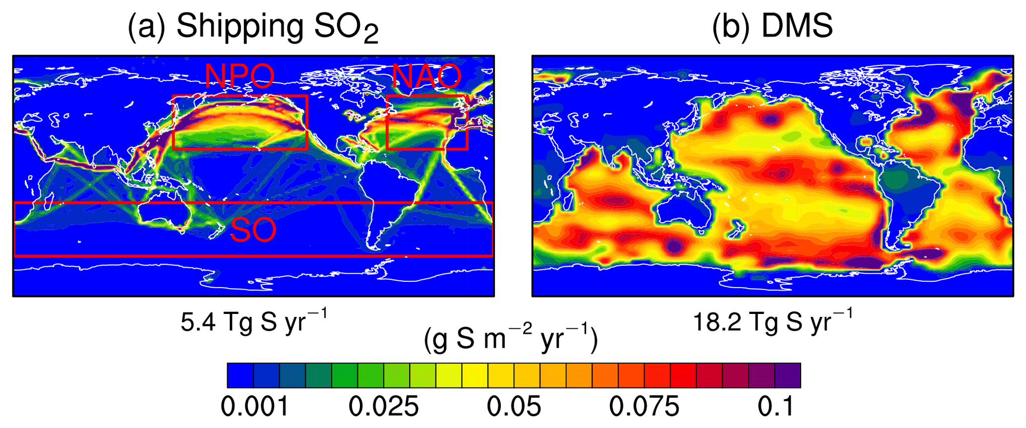
Figure 1Spatial patterns of annual means of sulfur emissions (g S m−2 yr−1) from (a) international shipping and (b) natural DMS in the simulation at the reference emission level (i.e., ShipRef_DMSRef). The numbers below each panel are the total global annual emissions. Three regions are selected for further analysis: the North Pacific Ocean (NPO; 20–60∘ N, 140–240∘ E), the North Atlantic Ocean (NAO; 20–60∘ N, 300–360∘ E), and the Southern Ocean (SO; 20–60∘ S, 0–360∘ E).
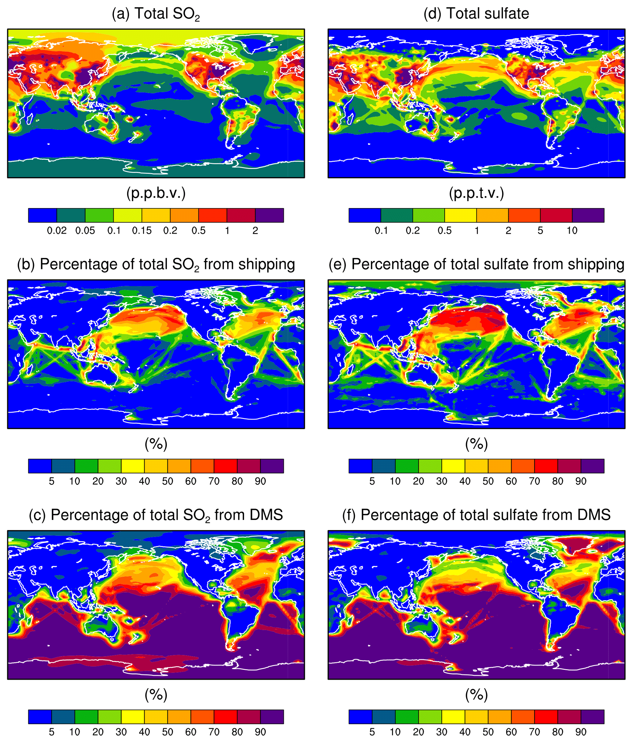
Figure 2Spatial patterns of (a) annual mean concentrations of total SO2 (parts per billion by volume; ppbv). Panels (b, c) show, respectively, the contributions of shipping emissions and natural DMS to total SO2 in the lowest model layer. Panels (d)–(f) are the same as (a)–(c), but for sulfate aerosols. These results are from MARC simulations and calculated as the differences between the simulations with the international shipping and DMS emissions at the reference and zero levels (i.e., ShipRef_DMSRef minus ShipZero_DMSRef and ShipRef_DMSRef minus ShipRef_DMSZero).
Sulfate aerosols are efficient cloud condensation nuclei (CCN) and control the formation of marine clouds and their micro- and macrophysical properties (McCoy et al., 2015). The international shipping-emitted sulfur dioxide from combustion of heavy fossil oil (Fig. 1) can be oxidized to sulfate aerosols that can increase cloud droplet number concentrations, cloud liquid water path, and planetary albedo, resulting in more solar radiation being reflected back to space, exerting a cooling effect on the climate system (Capaldo et al., 1999; Devasthale et al., 2006; Lauer et al., 2007, 2009). Although international shipping emissions (ISE) contribute only about 5 % (5.4 Tg S yr−1) to the total anthropogenic sulfur emissions (Corbett and Koehler, 2003; Endresen et al., 2005; Klimont et al., 2013), they dominate the sulfur concentration across much of the ocean, such as the North Pacific Ocean (NPO) and the North Atlantic Ocean (NAO), as shown in Fig. 2. Therefore, the radiative impact of the ISE via perturbing marine stratocumulus clouds could be large – especially because marine stratocumulus clouds are often collocated with busy shipping lanes (Neubauer et al., 2014). Note that although ISE also contain a significant amount of black carbon (BC) and organic carbon (OC) aerosols, since this study mainly focuses on aerosol-induced cloud radiative effect (CRE) instead of aerosol direct radiative effect (DRE), we focus on only primary and secondary sulfate aerosols due to their much higher hygroscopicity than those of BC and OC aerosols (Pringle et al., 2010).
The estimated global annual mean of the ISE-induced net CRE at the TOA has large uncertainties due to the complication in simulating clouds and aerosol–cloud interactions, ranging from −0.60 to −0.07 W m−2 (Capaldo et al., 1999; Lauer et al., 2007; Eyring et al., 2010; Righi et al., 2011; Peters et al., 2012, 2013; Partanen et al., 2013). Compared with net CRE, the net DRE of shipping emissions is much weaker, with a magnitude of only −0.08 to −0.01 W m−2, approximately 10 % of the former (Endresen et al., 2003; Schreier et al., 2007; Eyring et al., 2010).
In addition to shipping-emitted sulfur compounds, oceanic phytoplankton-derived dimethyl sulfide (DMS) is another significant component in the atmospheric sulfur cycle over oceans (Grandey and Wang, 2015; Mahajan et al., 2015; McCoy et al., 2015; Tesdal et al., 2016). DMS can be oxidized by hydroxyl radicals or nitrate radicals to produce sulfur dioxide and finally converted to sulfate aerosols (Boucher et al., 2003). The total global DMS emission is estimated to range from 8 to 51 Tg S yr−1 based on model simulation (Quinn et al., 1993; Dentener et al., 2006); this uncertainty range is itself substantially larger than the total sulfur emissions from shipping. The global annual mean of the DMS-induced net CRE at the TOA ranges from −2.03 to −1.49 W m−2 determined by DMS climatology (Gunson et al., 2006; Thomas et al., 2010; Mahajan et al., 2015).
Most of the aforementioned studies separately addressed the impacts on CRE of shipping and DMS emissions, largely ignoring the potential nonlinearity in the response of CREs to aerosol variations when these sulfate aerosols from two different sources such as the NPO and NAO often collocate in the marine atmosphere (Fig. 1). The nonlinearity between DMS emission and the associated CRE was studied previously without taking into account the shipping emissions (Pandis et al., 1994; Russell et al., 1994; Gunson et al., 2006; Thomas et al., 2011). Here, to evaluate the CRE induced by both ISE and DMS emissions with a consideration of their interactions, we selected three regions for detailed analysis: the NPO and NAO where the ISE dominate the concentrations of sulfur dioxide and sulfate aerosols and the Southern Ocean (SO) where DMS is the dominant source (Fig. 2).
This study employs an Earth system model including an interactive aerosol model that simultaneously resolves both external and internal mixtures of sulfate, BC, and OC aerosols. Aerosol mixing in this way can resolve aerosol activation processes more realistically than either mixing all aerosol species internally or ignoring any mixing at all. By comparing the results with the default aerosol scheme that assumes internal mixing, we also quantify the impacts of various assumptions of aerosol mixing states on estimates of the CRE of ISE and DMS emissions. We further quantify the ISE-induced CRE based on various regulations of the International Maritime Organization (IMO) on the fuel sulfur content. Therefore, our findings have important implications for policy makers and future estimates of CRE induced by both ISE and DMS emissions.
2.1 Climate model
The Community Earth System Model version 1.2.2 (CESM1.2.2) is configured with the Community Atmosphere Model version 5.3 (CAM5.3). CAM5.3 includes a modal aerosol model with an option of three or seven lognormal distributions of aerosol size (MAM3 or MAM7). In this study, a new modal aerosol model – the two-Moment, Multi-Modal, Mixing-state-resolving Aerosol model for Research of Climate (MARC; version 1.0.3 here) (Kim et al., 2008, 2014; Rothenberg and Wang, 2016, 2017; Grandey et al., 2018) – is introduced and used to evaluate both the DRE and CRE of ISE. The details of MARC are described below. Aerosol DREs are represented by coupling between aerosols and radiation. Aerosol CREs are included by activating aerosols to work as CCN and ice nuclei in the stratiform clouds (Morrison and Gettelman, 2008; Gettelman et al., 2010). Parameterization of aerosol activation is based on particle size and hygroscopicity of aerosols. Similar to other climate models, CAM5 does not directly include aerosol's influence through microphysics on convective clouds, but it allows aerosols to influence convective clouds indirectly, such as by aerosol's effect on circulation, surface evapotranspiration, and so on.
2.2 MAM3
The default aerosol scheme in CESM 1.2.2, MAM3, has three modes, each with a lognormal size distribution: Aitken, accumulation, and coarse. Various aerosol species are internally mixed within each mode. Aitken mode is a mixture of sulfate, secondary OC and sea salt; accumulation mode is mixture of sulfate, BC, primary OC, secondary OC, dust, and sea salt; coarse mode is a mixture of dust, sea salt, and sulfate (Liu et al., 2012). MAM3 tracks both the mass concentration and the number concentration of each aerosol mode.
2.3 MARC
MARC uses seven modes with different lognormal size distributions to represent the population of sulfate and carbonaceous aerosols: three modes for pure sulfate (nucleation or NUC, Aitken or AIT, and accumulation or ACC), one each for pure BC and pure OC, one mixture of BC–sulfate in core–shell structure (MBS), and one mixture of OC–sulfate (internal mixture; MOS). MARC predicts total particle mass and number concentrations while assuming the standard deviation within each of the seven modes to define at any given time the lognormal distribution of particle size. In addition, carbonaceous mass concentrations inside MBS and MOS are also predicted to allow the mass ratios between sulfate and carbonaceous compositions to evolve over time, changing the optical and chemical properties of the mixed aerosols. The emissions of mineral dust and sea salt that MARC uses are calculated by the land surface model and atmosphere model, respectively (Mahowald et al., 2006; Albani et al., 2014; Scanza et al., 2015). Mineral dust and sea salt are each represented by four bins with fixed sizes in MARC. For details of MARC aerosol mode size distribution and chemical parameters, please refer to Rothenberg and Wang (2017). Note that in the MARC model, gas-phase sulfur compounds can be oxidized in both the gaseous and aqueous phases to form sulfate that could enter the aerosol phase in several pathways: (1) aerosol nucleation to form new nucleation-mode sulfate aerosols; (2) condensation of gaseous sulfuric acid on both external sulfate and carbonaceous aerosols (the latter specifically ages carbonaceous aerosols to form sulfate–carbonaceous aerosol mixtures); and (3) evaporation of cloud and raindrops that resuspends aqueous sulfate to accumulation-mode sulfate aerosol (Kim et al., 2008; Grandey et al., 2018; Rothenberg et al., 2018).
2.4 Difference between MARC and MAM3
The most fundamental difference between MARC and MAM is that MARC includes both external and internal mixtures of aerosols in 15 modes while MAM treats all aerosols as internal mixtures in three modes. As a result, the processes of many aerosol microphysical processes including gaseous condensation, new particle formation, and nucleation scavenging differ between these two models (Kim et al., 2008; Grandey et al., 2018; Rothenberg et al., 2018).
For instance, aerosol activation or nucleation scavenging in MARC and MAM3 is calculated based on competition for water vapor among various types (or modes) of aerosols with different hygroscopicity. In this case, external sulfate modes and the mixture of BC and sulfate (MBS) with BC as core and sulfate as shell would have the same hygroscopicity as sulfate, while external BC and OC would have much lower hygroscopic values. Whereas, MAM calculates this process based on the volume weighted hygroscopicity of each mode based on all the aerosol constitutions within the mode. In that case, the change of individual aerosol species would not influence much the number of activated aerosol substantially (Rothenberg et al., 2018).
2.5 Radiation diagnostics
In the diagnostic mode of CESM–MARC, the DREs are diagnosed by calling the radiation scheme three times in each radiation time step. The first call does not include any aerosols, providing “clean-sky” diagnostics (Ghan, 2013). The second call includes only mineral dust and sea salt aerosols. The third call includes all aerosols. The first and third calls are diagnostic; i.e., the radiation budget calculated from these two calls is only used to as model output. Therefore they do not influence model integration in the next time step. Conversely, the second call is prognostic; i.e., the radiation budget from this call is passed to other model schemes to calculate associated model variables, such as temperature, surface evaporation, and so on. Therefore, DREs of only dust and sea salt aerosols are prognostic, while all other aerosols including ISE are diagnostic. Note that all radiation variables calculated in these three calls are stored in the model history files for further analyses. In the complimentary MAM3 simulations, the first radiation call (prognostic) includes all aerosols while the second call is a clean-sky diagnostic call, excluding all aerosols.
The DRE of aerosols is calculated by subtracting the TOA radiation in the clean-sky call (no direct aerosol–radiation interaction) from that in the call that includes all aerosols. The CRE is calculated by subtracting the TOA radiation at clear sky from that at all sky in the clean-sky call (Ghan, 2013). The calculation of the DRE and CRE of ISE takes a further step – subtracting the DRE and CRE in the simulation without ISE from that with ISE. In this way, the DRE and CRE of ISE can be isolated and evaluated separately. Note that all radiative effects are calculated at the TOA.
Table 1Summary of experiments.
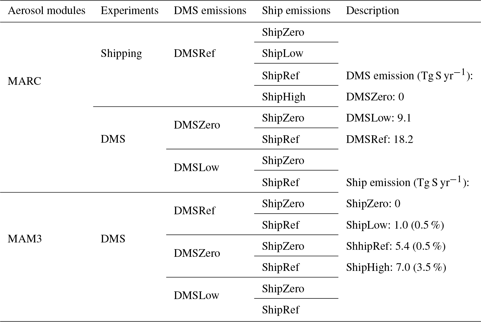
Note that in ShipZero experiments, emission rates of all gas-phase and aerosol species from shipping emissions are set to zero, while in ShipLow, ShipRef, and ShipHigh experiments, all shipping emission rates (such as OC and BC) are set to year-2000 values except for emission rates of sulfur compounds (i.e., SO2 and SO4), which are modified. The percent for ship emissions in the last column stands for the proportion of sulfur content in the heavy fuel oils by mass.
2.6 Experimental design
Three groups of simulations are designed to evaluate (a) the DRE and CRE of ISE and (b) the sensitivity of the ISE-induced CRE to both DMS emissions and aerosol mixing assumptions. CAM5 was run at a horizontal resolution of and 30 vertical layers with sea surface temperature (SST), sea ice, and greenhouse gas concentrations prescribed at the level of year 2000. The aerosol emissions in the year 2000 were used except for modified shipping and DMS emissions. The DMS emission is prescribed with a global annual average of 18.2 Tg S yr−1 in DMS reference simulations (Dentener et al., 2006). Each simulation runs for 32 years driven by 12-month cyclic climatological SST, with the first 2 years discarded as spin-up. Since the SSTs were prescribed, a 2-year period of spin-up should be enough for aerosol concentrations and other model components to reach an equilibrium state (e.g., Righi et al., 2011).
The first group uses CESM–MARC and includes four simulations, which share the same DMS reference emissions (DMSRef) while differing in four various ISE of sulfur compounds (sulfur dioxide and sulfate) (Table 1). The ShipZero_DMSRef simulation is integrated excluding all aerosol and aerosol precursor emissions from ISE, i.e., sulfur dioxide, sulfate aerosol, OC aerosol, and BC aerosol. The other three simulations – ShipLow_DMSRef, ShipRef_DMSRef, and ShipHigh_DMSRef – include the standard emissions of carbonaceous aerosols (e.g., BC and OC) while using three various emission scenarios of sulfur compounds from ISE. The three emission scenarios are based on the assumptions of sulfur content of the heavy fuel oils for oceangoing ships. Currently, the average sulfur content is 2.7 % (Corbett and Koehler, 2003; Endresen et al., 2005), which is equivalent to about 5.4 Tg S year−1, referred to as ShipRef. Conversely, as of 2013 the high-sulfur fuel oil that has a 3.5 % sulfur content continued to be permitted outside the Emission Control Areas (Lauer et al., 2009; Winebrake et al., 2009), referred to as ShipHigh. However, the IMO has planned to lower the sulfur content to 0.5 % outside the Emission Control Areas (Winebrake et al., 2009; Notteboom, 2010; International Maritime Organization, 2016) after 2020, referred to as ShipLow. In ShipLow and ShipHigh, the total global sulfur shipping emissions are 1.0 and 7.2 Tg S year−1, respectively. These numbers related to annual sulfur emissions are generally estimated based on the total amount of heavy fuel burnt by ships and the associated emission rates, whose uncertainties were addressed by Peters et al. (2012). The differences between these three and the zero-shipping-emissions scenarios represent how various regulations on marine fuel influence the ISE-induced CRE.
The second group also uses CESM–MARC and is comprised of three pairs of simulations: (ShipRef_DMSZero, ShipZero_DMSZero), (ShipRef_DMSLow, ShipZero_DMSLow), and (ShipRef_DMSRef, ShipZero_DMSRef). Note that the pair of (ShipRef_DMSRef, ShipZero_DMSRef) simulations is also part of the first group. The annual emission of DMS is 18.2 Tg S year−1 in the DMSRef simulations (Dentener et al., 2006; Liu et al., 2012) and half of that in the DMSLow simulations. DMS emission is excluded in the DMSZero simulations. Each pair of the simulations includes ShipZero and ShipRef, the difference of which represents the ISE-induced impacts. The purposes of the DMSZero and DMSLow simulations are to quantify the sensitivities of the ISE-induced CRE (i.e., the difference of CRE in each pair of simulations) to DMS emission and the associated large uncertainty in DMS emission, respectively (Quinn et al., 1993; Dentener et al., 2006). DMS emission in the DMSLow simulation is 9.1 Tg S year−1, which is close to the lower boundary of DMS emission estimates, i.e., 8 Tg S year−1 (Quinn et al., 1993). Such sensitivities are examined by calculating the differences among the three pairs of DMS simulations.
The third group is the same as the second, but using the default MAM3 aerosol module of CAM5.3 in CESM. The purpose for designing the third group is to cross-validate the simulated DMS impacts on the ISE-induced CRE in the second group. One bonus of the third group is to quantify the impacts of using different aerosol modules with different aerosol mixing states on the simulated results. The anthropogenic emissions for MAM3, which are described by Liu et al. (2012), differ slightly from those for MARC. All of the experiments are summarized in Table 1.
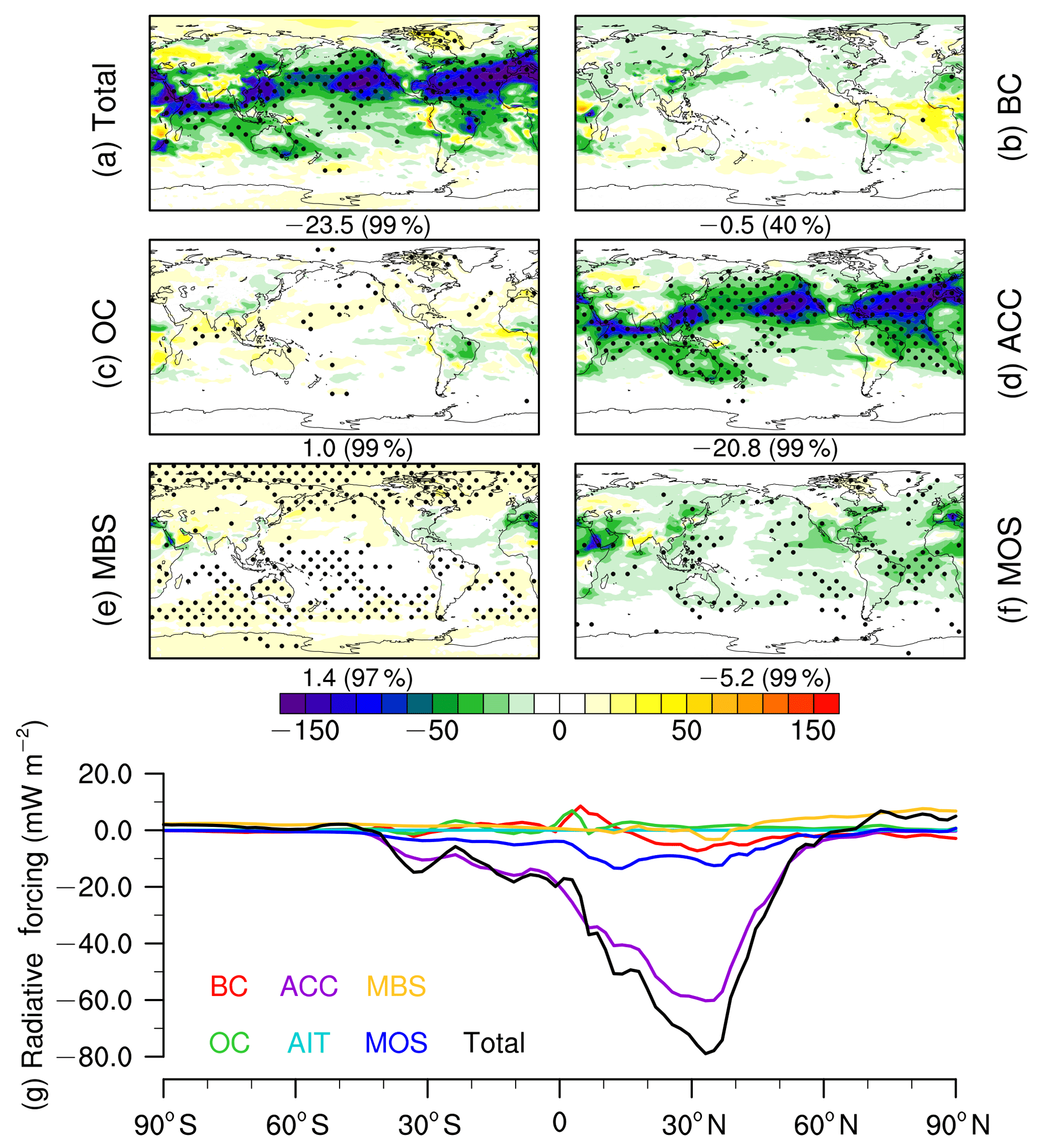
Figure 3Simulated direct radiative effect (DRE; mW m−2) of ISE at the TOA by MARC. The DRE is calculated as the difference between simulation results with and without ISE (i.e., ShipRef_DMSRef minus ShipZero_DMSRef) and averaged over the 30-year period of simulations at all-sky conditions. Panels (a)–(f) show the spatial patterns of DRE due to ISE with the global mean differences and the associated significant levels indicated by the numbers below each panel, and panel (g) shows the meridional variations in zonal mean DRE for various aerosol types from ISE and their total effects. The expansions of the abbreviations can be found in Sect. 2.3. The black dots represent grid points that are statistically significant above the 90 % confidence level based on the two-tailed Student's t test.
3.1 DRE of ISE
The all-sky DRE of various aerosol species from ISE is diagnosed as the difference between ShipRef_DMSRef and ShipZero_DMSRef and shown in Fig. 3. The total ISE can cause a global negative (cooling) DRE of −23.5 mW m−2, with the strongest negative (cooling) DRE in the areas with intense shipping tracks, such as midlatitude areas in the Pacific Ocean and Atlantic Ocean, South China Sea, north Indian Ocean, and the Red Sea. The sulfate aerosols in the accumulation mode (i.e., ACC) contribute 89 % to the global total DRE, followed by MOS aerosols with a contribution of 22 %. Note that OC and MBS have a counteracting warming effect (remember that all gas-phase and aerosol emissions from shipping have been removed in ShipZero scenarios). The contributions of other aerosol species are very limited and their magnitudes are smaller than 6 %. The magnitude of the total cooling effect is within the range from −50 to −10 mW m−2 estimated in previous studies (Endresen et al., 2003; Schreier et al., 2007). The meridional variations in global zonally averaged total DRE show that the DRE has the strongest cooling effect of −80 mW m−2 between 30 and 40∘ N and becomes weaker towards both polar regions and can be ignored beyond 45∘ S and 60∘ N. The all-sky DRE of total aerosols in ShipLow_DMSRef and ShipHigh_DMSRef has patterns similar to those in ShipRef_DMSRef and has magnitudes of +1.0 and −33.0 mW m−2, respectively. All of the calculated global DRE values except for BC are confident at the 90 % level.

Figure 4Spatial patterns of MARC-simulated cloud radiative effect (CRE; W m−2) at the TOA of ISE with various shipping emission levels. The CRE is calculated as the differences of radiation flux at the TOA and at all-sky conditions between the simulation without shipping emissions and three simulations with the same DMS emissions at the reference level but various shipping emission levels (i.e., low, reference, high) in short-wave (SW), long-wave (LW), and net (SW + LW) radiation and averaged over the 30-year simulation period. The numbers below each panel are the global means, standard deviation across the 30-year period, and the confidence level. The red dots represent grid points that are statistically significant above the 90 % confidence level based on the two-tailed Student's t test.
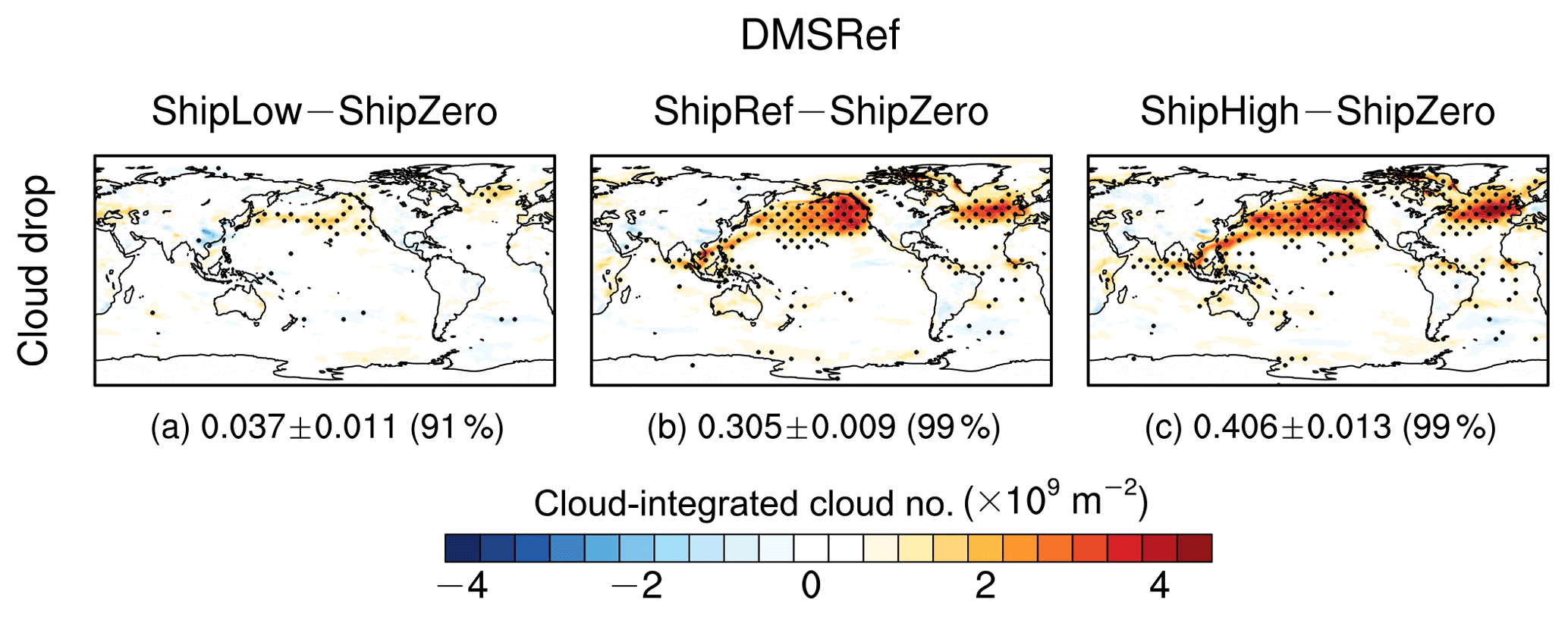
Figure 5Spatial patterns of MARC-simulated column-integrated cloud droplet number concentration (×109 m−2) response to international shipping emissions. The responses are calculated as the differences of cloud droplet number integrated through the whole atmospheric column between the simulation without shipping emissions and three simulations with the reference shipping emissions and various DMS emissions (i.e., zero, low, and reference) over the 30-year simulation period. The numbers below each panel are the global means, standard deviation across the 30-year period, and the confidence level. The black dots represent grid points that are statistically significant above the 90 % confidence level based on the two-tailed Student's t test.
3.2 CRE of ISE under various shipping emission regulations
The CRE of ISE is much stronger than the DRE and shows different spatial patterns under various shipping emission regulations (Fig. 4). At the reference level of shipping emissions (ShipRef_DMSRef), significant cooling CRE in shortwave (SW) radiation is simulated in areas of intense shipping tracks, such as the midlatitude Pacific Ocean and Baffin Bay between Canada and Greenland, with a global average of −0.218 W m−2. The longwave (LW) radiation CRE shows positive values in some small areas of high latitude, with a global average of +0.065 W m−2. Consequently, the global net CRE (SW + LW) is −0.153 W m−2 with a spatial pattern similar to that of SW radiation. At the high level of shipping emissions (ShipHigh_DMSRef), the CRE changes to −0.253, +0.073, and −0.179 W m−2 for SW, LW, and net radiation, respectively; more areas show significant changes than in ShipRef_DMSRef. Note that all of the above values are statistically significant above the 90 % confidence level. However, at the low level of shipping emissions (ShipLow_DMSRef), fewer areas demonstrate significant changes than in ShipRef_DMSRef and ShipHigh_DMSRef and the global averages of the CRE are not significant at the 90 % confidence level for SW and net radiation. These results indicate that more stringent shipping emission regulation on sulfur content decided by the IMO to be applied after 2020 could effectively reduce or even largely eliminate the net CRE induced by ISE.
Further analyses demonstrate that the changes in CRE are caused by perturbations in both cloud water path (CWP; Fig. S1 in the Supplement) and column-integrated cloud droplet number concentrations (CDNCs; Fig. 5) induced by ISE. Figure S1 demonstrates significant increases in total CWP mainly over the NPO and NAO at the reference and high levels of ISE. The increases in total CWP are largely (87 %) attributed to liquid CWP with the remaining contribution (13 %) from ice CWP at the reference shipping emission level. Such increases in CWP could reflect more solar radiation to space and thus cause a cooling radiative effect at the TOA, as shown in Fig. 4. Note that very limited areas in the NPO show significant increases in ice CWP, indicating that a small portion of surface shipping emissions could be vertically transported to very high altitude and form ice cloud. At the high level of shipping emissions, a larger increase in CWP is simulated, which is consistent with the cooler radiative effects. However, no significant changes are simulated in total, ice, or liquid CWP at the low level of shipping emissions. Associated with increases in CWP, the CDNC also illustrates significant increases at all levels of shipping emissions (Fig. 5), which collocate with increases in CWP (Fig. S1) and decreases in CRE (Fig. 4) over the NPO and NAO. The sulfate aerosols from shipping emissions are highly efficient CCN and thus can increase the CDNC, which in turn affects CWP. Note that cloud area fraction does not exhibit any significant changes due to shipping emissions (not shown).
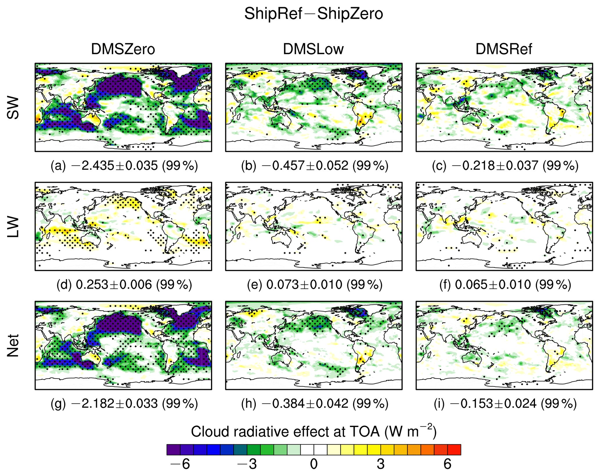
Figure 6Spatial patterns of MARC-simulated cloud radiative effect (CRE; W m−2) at the TOA of ISE at various DMS emission levels. The CRE is calculated as the differences of radiation flux at the TOA and at all-sky conditions between the simulation without shipping emissions and three simulations with the same shipping emissions at the reference level but various DMS emission levels (i.e., zero, low, and reference) in short-wave (SW), long-wave (LW), and net (SW + LW) radiation and averaged over the 30-year simulation period. The numbers below each panel are the global means, standard deviation across the 30-year period, and the confidence level. The black dots represent grid points that are statistically significant above the 90 % confidence level based on the two-tailed Student's t test.
3.3 CRE of ISE under various DMS emissions
The biogenic emissions of DMS over oceans can be oxidized to sulfates and compete against shipping-emitted sulfates for CCN and thus could influence the ISE-induced CRE. We find that the shipping-emissions-induced CRE exhibits significantly different patterns and global averages at different emission levels of DMS (Fig. 6). With DMS emissions ranging from the reference level to low and zero levels, the magnitude of the ISE-induced negative CRE at SW radiation increases from 0.218 to 0.457 and 2.435 W m−2 on a global scale, respectively; significant negative CRE is simulated over more areas in the SO. It is worth noting that the ISE-induced CRE can reach up to −6 W m−2 when DMS emission is turned off, such as over the NPO and NAO, which is a very large negative forcing even on the local scale. Since there are no comparable values in the literature, this large negative forcing warrants a detailed evaluation in future studies using different climate models. For CRE at LW radiation, more areas with significant warming are seen in the SO, NPO, and NAO, with the global averages changing from +0.065 to +0.073 and +0.253 W m−2 when DMS emissions change from the reference to low and zero levels, respectively. Net CRE shares similar features with those at SW radiation, but with smaller magnitudes.
The DMS emissions influence the ISE-induced CRE by perturbing the ISE-induced changes in CWP and column-integrated CDNC (Figs. S2 and 7). The shipping-emissions-induced changes in the total and liquid CWP increase as DMS emission decreases, particularly over the SO, the NPO, and the NAO, while no significant changes are simulated in the ice CWP. The increased CWP is closely associated with the increases in the column-integrated CDNC, which changes from 0.305×10⁹ m−2 (2.5 %, relative to climatological CDNC in the ShipZero_DMSRef simulation) to 0.476×10⁹ m−2 (3.9 %) and 0.999×10⁹ m−2 (8.3 %) on a global scale as DMS emission decreases. These results imply that DMS emissions are the dominant sources of cloud seeds over remote oceans. The most prominent increases in CDNC are seen in the SO, NPO, and NAO. These results suggest important roles of DMS emissions in modulating the ISE-induced changes in cloud properties and radiation. Note that cloud area fraction does not exhibit any significant change (not shown).
As demonstrated in the above analysis, the impacts of DMS emissions on cloud response to shipping emissions are the most prominent over the SO, the NPO, and the NAO, so further analyses are performed over these three regions. Figure 8 shows cloud responses to shipping emissions at different DMS emission levels over the three oceanic regions. Generally, cloud responses become weaker and weaker as DMS emission increases from zero (DMSZero) to low (DMSLow) and reference (DMSRef) level over all three regions. The most prominent change in cloud response is over the NPO, followed by the NAO and the SO, which is probably due to the higher contribution of shipping emissions to the total sulfur dioxide and sulfate aerosols over the NPO than the NAO and the SO (Fig. 2b and e). The removal of DMS emission (DMSZero) has a much stronger influence on cloud response to shipping emissions than reducing DMS emission by half (DMSLow), indicating a strong nonlinear competing effect for CCN between DMS and shipping emissions.
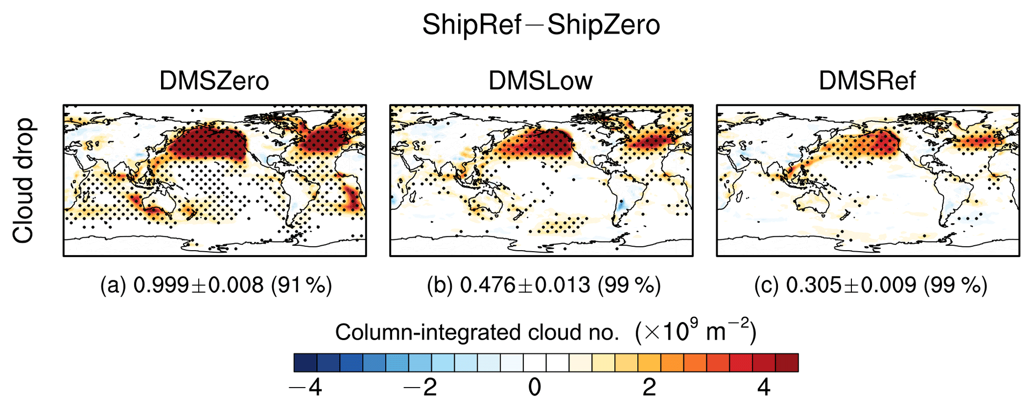
Figure 7Spatial patterns of MARC-simulated column-integrated cloud droplet number concentration (×109 m−2) response to international shipping emissions. The responses are calculated as the differences of cloud droplet number integrated through the whole atmospheric column between the simulation without shipping emissions and three simulations with the reference shipping emissions and various DMS emissions (i.e., zero, low, and reference) over the 30-year simulation period. The numbers below each panel are the global means, standard deviation across the 30-year period, and the confidence level. The black dots represent grid points that are statistically significant above the 90 % confidence level based on the two-tailed Student's t test.

Figure 8Impacts of DMS emissions on cloud responses to international shipping emissions. (a) Cloud radiative effects at the TOA (W m−2), (b) column-integrated cloud water path (g m−2), and (c) column-integrated cloud droplet number (×109 m−2). The green, purple, and blue curves respectively represent quantities area-averaged over the North Pacific Ocean (NPO), the North Atlantic Ocean (NAO), and the Southern Ocean (SO), which are shown as red boxes in Fig. 1a. These results are from MARC simulations.
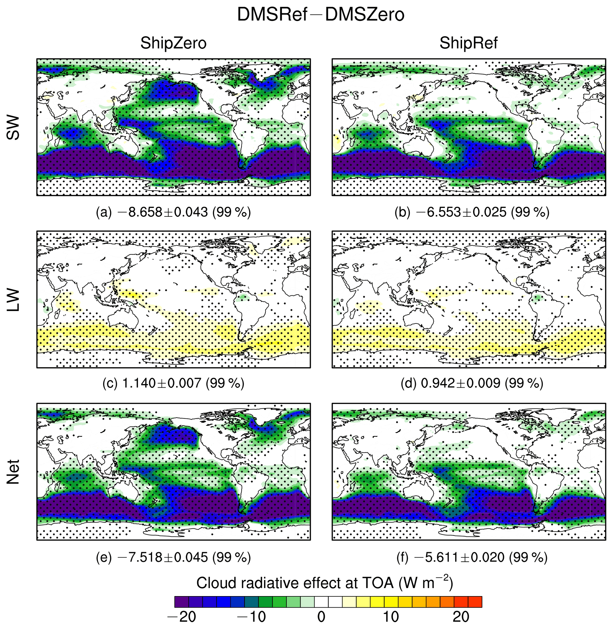
Figure 9Spatial patterns of MARC-simulated cloud radiative effect (W m−2) of DMS emissions at various shipping emission levels. The CRE is calculated as the differences of radiation flux at the TOA and at all-sky conditions between the simulation without DMS emissions and two simulations with the same DMS emissions at the reference level but various shipping emission levels (i.e., zero and reference) in short-wave (SW), long-wave (LW), and net (SW + LW) radiation and averaged over the 30-year simulation period. The numbers below each panel are the global means, standard deviation across the 30-year period, and the confidence level. The black dots represent grid points that are statistically significant above the 90% confidence level based on the two-tailed Student's t test.

Figure 10Impacts of ISE on cloud responses to DMS emissions. (a) Cloud radiative effects at the TOA (W m−2), (b) column-integrated cloud water path (g m−2), and (c) column-integrated cloud droplet number (×109 m−2). The green, purple, and blue curves respectively represent quantities area-averaged over the North Pacific Ocean (NPO), the North Atlantic Ocean (NAO), and the Southern Ocean (SO), which are shown as red boxes in Fig. 1a. These results are from MARC simulations.
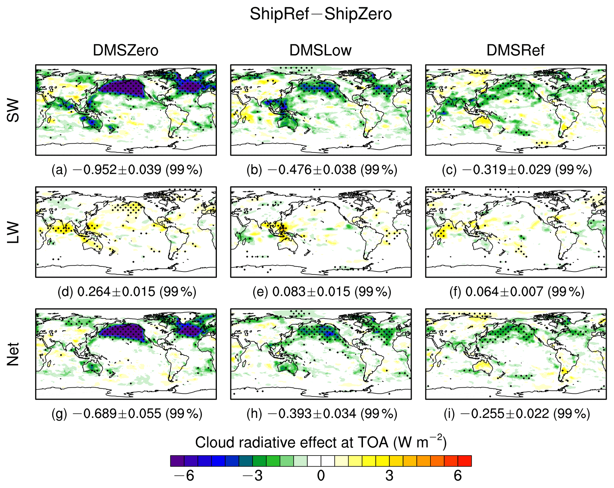
Figure 11Same as Fig. 6, but using a different aerosol module, namely MAM3 rather than MARC.
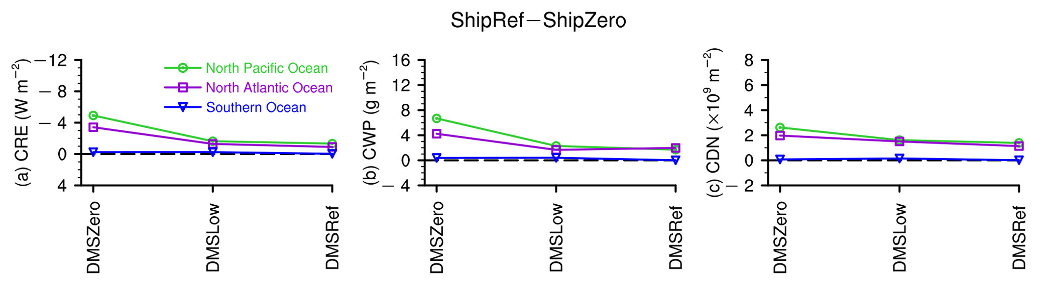
Figure 12Same as Fig. 8, but using a different aerosol module, namely MAM3 rather than MARC.
3.4 CRE of DMS under various shipping emissions
Similar to DMS emissions' impacts on the ISE-induced CRE and cloud properties, ISE could also influence the DMS emission-induced CRE and cloud properties. Generally, stronger cooling net CREs (−7.518 vs. −5.611 W m−2) induced by DMS emissions are seen when shipping emissions are absent, particularly in areas of intense shipping tracks, such as over the NPO and the NAO (Fig. 9). Such a net cooling CRE is mainly the result of SW CRE. Stronger cooling CRE is associated with larger increases in liquid and total CWP (Fig. S3) and column-integrated CDNC (Fig. S4) in simulations without shipping emissions than those with shipping emissions.
It is worth pointing out that DMS emissions have a significant warming CRE at LW radiation, particularly over midlatitude and high-latitude regions in the Southern Hemisphere and high-latitude regions in the Northern Hemisphere regardless of the presence of shipping emissions (Fig. 9). Such a warming CRE could be attributed to increases in total cloud area fraction, which is further attributed to increases in the middle and low cloud area fraction in the high-latitude regions in both hemispheres (Fig. S5). Our results indicate that DMS is a significant source to CCN in the extremely clean polar regions in both hemispheres.
The area-averaged cloud responses over the SO, the NPO, and the NAO to DMS emissions at different shipping emission levels are shown in Fig. 10. Cloud responses to DMS are stronger over the SO than over the NPO and the NAO regardless of the presence of shipping emissions due to the fact that DMS and shipping emissions respectively dominate the sulfur concentrations over the SO and the NPO and the NAO (Fig. 2). Moreover, cloud responses to DMS emissions become much stronger over all three oceanic regions when shipping emissions have been removed. However, such changes in cloud responses to DMS due to removal of shipping emissions (i.e., the slopes of the curves) are stronger over the NPO and the NAO than over the SO, which is caused by very limited shipping emissions over the SO. These results again indicate a strong nonlinear competing effect for CCN between DMS and shipping emissions.
3.5 Impacts of choice of aerosol module on the results
In addition to the impacts of various ISE regulations and DMS emissions on the ISE-induced CRE, various assumptions about the aerosol mixing states could also have an impact. Figure 11 shows the same results as Fig. 6 but using the MAM3 aerosol module instead of MARC. At the reference level of DMS emissions (DMSRef), the ISE-induced CREs are generally stronger in MAM3 (SW: −0.319, LW: +0.064, and net: −0.255 W m−2; Fig. 11) than in MARC for SW and net radiation (SW: −0.218, LW: +0.065, net: −0.153 W m−2; Fig. 6). More areas with a significant cooling CRE are simulated in MAM3 than in MARC, particularly in the Atlantic Ocean, west Pacific Ocean, and north Indian Ocean. At the low level of DMS emissions (DMSLow), both the global averages and spatial patterns of the CRE in MAM3 are very similar to those in MARC. The two aerosol modules show the biggest differences in CRE when DMS emissions are excluded (DMSZero). MARC simulates strong ISE-induced CRE over tropical regions and the subtropical and midlatitude areas of the SO, while MAM3 gives no significant CRE over these regions. Generally, the ISE-induced CRE is stronger in MARC than in MAM3 when DMS emissions are excluded. The associated changes in CDNC and CWP due to ISE illustrate patterns similar to changes in CRE (Figs. S6 and S7). A possible reason for such differences is the various mixing assumptions about sulfate and sea salt aerosols in MARC (external mixing) versus in MAM3 (internal mixing). Interested readers are referred to Grandey et al. (2018) for discussion of the differing radiative effects produced by MARC and MAM. To track down all the possible reasons for the differences in the ISE-induced CRE between the two aerosol schemes, more detailed analyses on a long chain of processes related to both aerosols and clouds are required, as carried out by Peters et al. (2014), which is out of the scope of this study and warrants more studies in the future.
By comparing Fig. 8 with Fig. 12 we also observe significantly different impacts of DMS emissions on cloud response to shipping emissions (i.e., the slopes of these curves). MAM3 simulates a weaker impact of DMS emissions on cloud response to shipping emissions than MARC, indicating a weaker nonlinear competing effect for CCN between DMS and shipping emissions in MAM3 than MARC.
Aerosols from ISE could exert significant cooling on the Earth's climate system through aerosol–cloud and aerosol–radiation interactions. To reduce the pollution and climatic effects from this emission source, the IMO set various emission caps on sulfur content of marine fuel oil to be implemented in the future. Using a state-of-the-art climate model, we find that the newly proposed more stringent emission regulations of shipping emissions can effectively reduce the ISE-induced CRE. As demonstrated in our results, reducing sulfur contents from 3.5 % to 2.7 % and 0.5 % could reduce both DRE (from −51.4 to −36.7 and −3.9 mW m−2) and CRE (from −0.179 to −0.153 and −0.001 W m−2) due to ISE, respectively. Although the ISE-induced CRE would be insignificant on a global scale if sulfur contents of ship fuels were reduced to 0.5 %, over some regions significant CREs can still be detected – e.g., high-latitude regions of the eastern Pacific Ocean. Therefore, implementation of cleaner fuels, such as natural gas, in the shipping sector could be a potential solution for completely eliminating sulfate-induced CREs.
More importantly, we find that the magnitude and regional spatial pattern of the ISE-induced CRE are highly sensitive to natural DMS emissions. With DMS emissions reducing from 18.2 to 9.1 Tg S yr−1 and zero, the ISE-induced net CRE changes from −0.153 to −0.384 and −2.182 W m−2, respectively. Conversely, the DMS-induced net CRE changes from −5.611 to −7.518 W m−2 when shipping emissions at the reference level are removed in the simulations. It is worth noting that DMS is a significant source to CCN in the extremely clean polar regions in both hemispheres. The strong interactions of CRE between DMS and shipping emissions can be attributed to the nonlinearity in the responses of cloud processes to aerosols, particularly the aerosol activation parameterizations (Abdul-Razzak et al., 1998). In a relatively clean environment, activated aerosol number concentration increases as ambient aerosol number concentration increases until reaching a peak at a specific aerosol number concentration, after which it decreases as ambient aerosol number concentration increases unless ambient vapor concentration is drastically increased. In other words, the fraction of activated aerosols decreases as ambient aerosol concentration increases (Fig. S8). From the perspective of simulation, this nonlinearity in aerosol activation strongly suggests a reevaluation of CRE induced by shipping and DMS emissions as well as a reevaluation of parameterizations of aerosol–cloud interactions in general circulation models. From the perspective of field measurements of aerosol–cloud relationships, it warrants careful attention when selecting measurement locations – shipping-emissions-related measurements should be collected along intense shipping tracks while in areas with as low of DMS emissions as possible to avoid contamination from DMS, and vice versa. Moreover, locations containing both shipping and DMS emissions should also be identified and sampled in order to investigate nonlinear interactions between the emissions.
Finally, we find that two different aerosol schemes, with different representations of aerosol mixing state, could produce a large difference (about 67 %) in the ISE-induced global CRE. Generally, the MARC aerosol module shows a stronger nonlinear cloud response to DMS and shipping emissions than MAM3. Overall, numerical studies on the uncertainties in the shipping-emissions-induced CRE due to various ISE regulations, aerosol interactions, and aerosol mixing states can provide useful information for policy makers and have implications for future projections of anthropogenic climate change.
In addition to the abovementioned contributors to the uncertainty in estimating the CRE induced by shipping emissions, spatial resolution of the model is another significant source of this uncertainty. Possner et al. (2016) found that the ship-induced shortwave CRE could increase by a factor of 2 as model spatial resolution decreases from 1 to 50 km. With higher spatial resolution, models can resolve fine-scale dynamical processes and feedbacks, such as interaction between aerosol and cumulus clouds (Malavelle et al., 2017). Though model-resolution-induced uncertainty is not the focus of this study, it should be taken into account when interpreting the spread of shipping-induced CRE in studies of multi-model comparison.
Though we employed a state-of-the-art climate model in this study, it is not without caveats, given that neither the MARC nor MAM (including both MAM3 and MAM7 in CAM5) aerosol modules treat nitrate aerosols because of the high computational expense for related aerosol–gaseous chemistry and aerosol thermodynamics calculations (Liu et al., 2012). Lack of treating nitrate aerosols could result in uncertainties in our results based on the fact that both mass of nitrate aerosols emitted from international shipping (e.g., Righi et al., 2011) and their hygroscopicity values (e.g., Kawecki and Steiner, 2018) are very similar to those of sulfate aerosols, and thus nitrate aerosols could have non-negligible competing effects on CRE with sulfate aerosols. Despite that some of the results from this study could be used to qualitatively project the potential outcome, a quantitative assessment should be facilitated to address this topic with an improved model.
The MARC source code is available via https://github.mit.edu/marc/marc_cesm/ and also archived with DOI https://doi.org/10.5281/zenodo.1117370 (Avramov et al., 2017), along with documentation on how to install and run the model. The version 23e08fe was used in this study. The model output data are archived with DOI https://doi.org/10.6084/m9.figshare.7370846.v1 (Jin et al., 2018a). The scripts used to post-process the model output data and create figures are archived with DOI https://doi.org/10.5281/zenodo.1493453 (Jin et al., 2018b).
The supplement related to this article is available online at: https://doi.org/10.5194/acp-18-16793-2018-supplement.
AA and DR coupled MARC to CAM5.3 in CESM1.2.2 under supervision of CW. QJ and CW designed the experiments with help from BSG and DR. QJ and BSG respectively performed CESM-MARC and CESM-MAM3 simulations. QJ analyzed the model results and wrote the paper with contributions from all other co-authors.
The authors declare that they have no conflict of interest
This study is supported by Concawe, whose mission is to conduct research on environmental issues relevant to the oil refining industry. This research is also partially supported by the US National Science Foundation (AGS-1339264), the U.S. Department of Energy (DE-FG02-94ER61937), and the National Research Foundation (NRF) of Singapore under its Campus for Research Excellence and Technological Enterprise program. The Center for Environmental Sensing and Modeling (CENSAM) is an interdisciplinary research group of the Singapore-MIT Alliance for Research and Technology (SMART). The CESM project is supported by the National Science Foundation and the Office of Science (BER) of the U.S. Department of Energy. We would like to acknowledge high-performance computing support from Yellowstone (ark:/85065/d7wd3xhc) provided by NCAR's Computational and Information Systems Laboratory, sponsored by the National Science Foundation. Edited by: Michael Schulz Reviewed by: two anonymous referees
Abdul-Razzak, H., Ghan, S. J., and Rivera-Carpio, C.: A parameterization of aerosol activation – 1. Single aerosol type, J. Geophys. Res.-Atmos., 103, 6123–6131, 1998.
Albani, S., Mahowald, N. M., Perry, A. T., Scanza, R. A., Zender, C. S., Heavens, N. G., Maggi, V., Kok, J. F., and Otto-Bliesner, B. L.: Improved dust representation in the Community Atmosphere Model, J. Adv. Model Earth Sy., 6, 541–570, 2014.
Avramov, A., Rothenberg, D., Jin, Q., Garimella, S., Grandey, B., and Wang, C.: MARC – Model for Research of Aerosols and Climate (Version v1.0.4), Zenodo, https://doi.org/10.5281/zenodo.1117370, 17 December 2017.
Boucher, O., Moulin, C., Belviso, S., Aumont, O., Bopp, L., Cosme, E., von Kuhlmann, R., Lawrence, M. G., Pham, M., Reddy, M. S., Sciare, J., and Venkataraman, C.: DMS atmospheric concentrations and sulphate aerosol indirect radiative forcing: a sensitivity study to the DMS source representation and oxidation, Atmos. Chem. Phys., 3, 49–65, https://doi.org/10.5194/acp-3-49-2003, 2003.
Boucher, O., Randall, D., Artaxo, P., Bretherton, C., Feingold, G., Forster, P., Kerminen, V.-M., Kondo, Y., Liao, H., Lohmann, U., Rasch, P., Satheesh, S. K., Sherwood, S., Stevens, B., and Zhang, X. Y.: Clouds and Aerosols, in: Climate Change 2013: The Physical Science Basis. Contribution of Working Group I to the Fifth Assessment Report of the Intergovernmental Panel on Climate Change, edited by: Stocker, T. F., Qin, D., Plattner, G.-K., Tignor, M., Allen, S. K., Boschung, J., Nauels, A., Xia, Y., Bex, V., and Midgley, P. M., Cambridge University Press, Cambridge, United Kingdom and New York, NY, USA, 571–658, 2013.
Capaldo, K., Corbett, J. J., Kasibhatla, P., Fischbeck, P., and Pandis, S. N.: Effects of ship emissions on sulphur cycling and radiative climate forcing over the ocean, Nature, 400, 743–746, 1999.
Corbett, J. J. and Koehler, H. W.: Updated emissions from ocean shipping, J. Geophys Res., 108, 4650, https://doi.org/10.1029/2003JD003751, 2003.
Dentener, F., Kinne, S., Bond, T., Boucher, O., Cofala, J., Generoso, S., Ginoux, P., Gong, S., Hoelzemann, J. J., Ito, A., Marelli, L., Penner, J. E., Putaud, J.-P., Textor, C., Schulz, M., van der Werf, G. R., and Wilson, J.: Emissions of primary aerosol and precursor gases in the years 2000 and 1750 prescribed data-sets for AeroCom, Atmos. Chem. Phys., 6, 4321–4344, https://doi.org/10.5194/acp-6-4321-2006, 2006.
Devasthale, A., Krüger, O., and Graßl, H.: Impact of ship emissions on cloud properties over coastal areas, Geophys. Res. Lett., 33, L02811, https://doi.org/10.1029/2005GL024470, 2006.
Endresen, O., Sorgard, E., Sundet, J. K., Dalsoren, S. B., Isaksen, I. S. A., Berglen, T. F., and Gravir, G.: Emission from international sea transportation and environmental impact, J. Geophys. Res., 108, 4560, https://doi.org/10.1029/2002JD002898, 2003.
Endresen, O., Bakke, J., Sorgard, E., Berglen, T. F., and Holmvang, P.: Improved modelling of ship SO2 emissions – a fuel-based approach, Atmos. Environ., 39, 3621–3628, 2005.
Eyring, V., Isaksen, I. S. A., Berntsen, T., Collins, W. J., Corbett, J. J., Endresen, O., Grainger, R. G., Moldanova, J., Schlager, H., and Stevenson, D. S.: Transport impacts on atmosphere and climate: Shipping, Atmos. Environ., 44, 4735–4771, 2010.
Gettelman, A., Liu, X., Ghan, S. J., Morrison, H., Park, S., Conley, A. J., Klein, S. A., Boyle, J., Mitchell, D. L., and Li, J. L. F.: Global simulations of ice nucleation and ice supersaturation with an improved cloud scheme in the Community Atmosphere Model, J. Geophys. Res., 115, D18216, https://doi.org/10.1029/2009JD013797, 2010.
Ghan, S. J.: Technical Note: Estimating aerosol effects on cloud radiative forcing, Atmos. Chem. Phys., 13, 9971–9974, https://doi.org/10.5194/acp-13-9971-2013, 2013.
Grandey, B. S. and Wang, C.: Enhanced marine sulphur emissions offset global warming and impact rainfall, Sci. Rep., 5, 13055, https://doi.org/10.1038/srep13055, 2015.
Grandey, B. S., Rothenberg, D., Avramov, A., Jin, Q., Lee, H.-H., Liu, X., Lu, Z., Albani, S., and Wang, C.: Effective radiative forcing in the aerosol–climate model CAM5.3-MARC-ARG, Atmos. Chem. Phys., 18, 15783–15810, https://doi.org/10.5194/acp-18-15783-2018, 2018.
Gunson, J. R., Spall, S. A., Anderson, T. R., Jones, A., Totterdell, I. J., and Woodage, M. J.: Climate sensitivity to ocean dimethylsulphide emissions, Ge ophys. Res. Lett., 33, L07701, https://doi.org/10.1029/2005GL024982, 2006.
International Maritime Organization: IMO sets 2020 date for ships to comply with low sulphur fuel oil requirement, avalable at: http://www.imo.org/en/MediaCentre/PressBriefings/Pages/MEPC-70-2020sulphur.aspx (last access: 21 November 2018), 2016.
Jin, Q.: Data for “Impacts on cloud radiative effects induced by coexisting aerosols converted from international shipping and maritime DMS emissions”, figshare, https://doi.org/10.6084/m9.figshare.7370846.v1, 21 November 2018a.
Jin, Q.: Analysis and plot NCL scripts for “Impacts on cloud radiative effects induced by coexisting aerosols converted from international shipping and maritime DMS emissions” (Version V1), Zenodo, https://doi.org/10.5281/zenodo.1493453, 21 November 2018b.
Kawecki, S. and Steiner, A. L.: The Influence of Aerosol Hygroscopicity on Precipitation Intensity During a Mesoscale Convective Event, J. Geophys. Res.-Atmos., 123, 424–442, 2018.
Kim, D., Wang, C., Ekman, A. M. L., Barth, M. C., and Rasch, P. J.: Distribution and direct radiative forcing of carbonaceous and sulfate aerosols in an interactive size-resolving aerosol-climate model, J. Geophys. Res., 113, D16309, https://doi.org/10.1029/2007JD009756, 2008.
Kim, D., Wang, C., Ekman, A. M. L., Barth, M. C., and Lee, D. I.: The responses of cloudiness to the direct radiative effect of sulfate and carbonaceous aerosols, J. Geophys. Res.-Atmos., 119, 1172–1185, 2014.
Klein, S. A. and Hartmann, D. L.: The Seasonal Cycle of Low Stratiform Clouds, J. Climate, 6, 1587–1606, 1993.
Klimont, Z., Smith, S. J., and Cofala, J.: The last decade of global anthropogenic sulfur dioxide: 2000–2011 emissions, Environ. Res. Lett., 8, 014003, https://doi.org/10.1088/1748-9326/8/1/014003, 2013.
Lauer, A., Eyring, V., Hendricks, J., Jöckel, P., and Lohmann, U.: Global model simulations of the impact of ocean-going ships on aerosols, clouds, and the radiation budget, Atmos. Chem. Phys., 7, 5061–5079, https://doi.org/10.5194/acp-7-5061-2007, 2007.
Lauer, A., Eyring, V., Corbett, J. J., Wang, C. F., and Winebrake, J. J.: Assessment of Near-Future Policy Instruments for Oceangoing Shipping: Impact on Atmospheric Aerosol Burdens and the Earth's Radiation Budget, Environ. Sci. Technol., 43, 5592–5598, 2009.
Liu, X., Easter, R. C., Ghan, S. J., Zaveri, R., Rasch, P., Shi, X., Lamarque, J.-F., Gettelman, A., Morrison, H., Vitt, F., Conley, A., Park, S., Neale, R., Hannay, C., Ekman, A. M. L., Hess, P., Mahowald, N., Collins, W., Iacono, M. J., Bretherton, C. S., Flanner, M. G., and Mitchell, D.: Toward a minimal representation of aerosols in climate models: description and evaluation in the Community Atmosphere Model CAM5, Geosci. Model Dev., 5, 709–739, https://doi.org/10.5194/gmd-5-709-2012, 2012.
Mahajan, A. S., Fadnavis, S., Thomas, M. A., Pozzoli, L., Gupta, S., Royer, S. J., Saiz-Lopez, A., and Simó, R.: Quantifying the impacts of an updated global dimethyl sulfide climatology on cloud microphysics and aerosol radiative forcing, J. Geophys. Res.-Atmos., 120, 2524–2536, 2015.
Mahowald, N. M., Muhs, D. R., Levis, S., Rasch, P. J., Yoshioka, M., Zender, C. S., and Luo, C.: Change in atmospheric mineral aerosols in response to climate: Last glacial period, preindustrial, modern, and doubled carbon dioxide climates, J. Geophys. Res., 111, D10202, https://doi.org/10.1029/2005JD006653, 2006.
Malavelle, F. F., Haywood, J. M., Jones, A., Gettelman, A., Clarisse, L., Bauduin, S., Allan, R. P., Karset, I. H. H., Kristjansson, J. E., Oreopoulos, L., Cho, N., Lee, D., Bellouin, N., Boucher, O., Grosvenor, D. P., Carslaw, K. S., Dhomse, S., Mann, G. W., Schmidt, A., Coe, H., Hartley, M. E., Dalvi, M., Hill, A. A., Johnson, B. T., Johnson, C. E., Knight, J. R., O'Connor, F. M., Partridge, D. G., Stier, P., Myhre, G., Platnick, S., Stephens, G. L., Takahashi, H., and Thordarson, T.: Strong constraints on aerosol-cloud interactions from volcanic eruptions, Nature, 546, 485491, https://doi.org/10.1038/nature22974, 2017.
McCoy, D. T., Burrows, S. M., Wood, R., Grosvenor, D. P., Elliott, S. M., Ma, P.-L., Rasch, P. J., and Hartmann, D. L.: Natural aerosols explain seasonal and spatial patterns of Southern Ocean cloud albedo, Science Advances, 1, e1500157, https://doi.org/10.1126/sciadv.1500157, 2015.
Morrison, H. and Gettelman, A.: A new two-moment bulk stratiform cloud microphysics scheme in the community atmosphere model, version 3 (CAM3). Part I: Description and numerical tests, J. Climate, 21, 3642–3659, 2008.
Neubauer, D., Lohmann, U., Hoose, C., and Frontoso, M. G.: Impact of the representation of marine stratocumulus clouds on the anthropogenic aerosol effect, Atmos. Chem. Phys., 14, 11997–12022, https://doi.org/10.5194/acp-14-11997-2014, 2014.
Notteboom, T.: The impact of low sulphur fuel requirements in shipping on the competitiveness of roro shipping in Northern Europe, WMU Journal of Maritime Affairs, 10, 63–95, https://doi.org/10.1007/s13437-010-0001-7, 2010.
Pandis, S. N., Russell, L. M., and Seinfeld, J. H.: The Relationship between Dms Flux and Ccn Concentration in Remote Marine Regions, J. Geophys. Res., 99, 16945–16957, https://doi.org/10.1029/94JD01119, 1994.
Partanen, A. I., Laakso, A., Schmidt, A., Kokkola, H., Kuokkanen, T., Pietikäinen, J.-P., Kerminen, V.-M., Lehtinen, K. E. J., Laakso, L., and Korhonen, H.: Climate and air quality trade-offs in altering ship fuel sulfur content, Atmos. Chem. Phys., 13, 12059–12071, https://doi.org/10.5194/acp-13-12059-2013, 2013.
Peters, K., Stier, P., Quaas, J., and Graßl, H.: Aerosol indirect effects from shipping emissions: sensitivity studies with the global aerosol-climate model ECHAM-HAM, Atmos. Chem. Phys., 12, 5985–6007, https://doi.org/10.5194/acp-12-5985-2012, 2012.
Peters, K., Stier, P., Quaas, J., and Graßl, H.: Corrigendum to “Aerosol indirect effects from shipping emissions: sensitivity studies with the global aerosol-climate model ECHAM-HAM” published in Atmos. Chem. Phys., 12, 5985–6007, 2012, Atmos. Chem. Phys., 13, 6429–6430, https://doi.org/10.5194/acp-13-6429-2013, 2013.
Peters, K., Quaas, J., Stier, P., and Graßl, H.: Processes limiting the emergence of detectable aerosol indirect effects on tropical warm clouds in global aerosol-climate model and satellite data, Tellus B, 66, 24054, https://doi.org/10.3402/tellusb.v66.24054, 2014.
Possner, A., Zubler, E., Lohmann, U., and Schär, C.: The resolution dependence of cloud effects and ship-induced aerosol-cloud interactions in marine stratocumulus, J. Geophys. Res.-Atmos., 121, 4810–4829, https://doi.org/10.1002/2015jd024685, 2016.
Pringle, K. J., Tost, H., Pozzer, A., Pöschl, U., and Lelieveld, J.: Global distribution of the effective aerosol hygroscopicity parameter for CCN activation, Atmos. Chem. Phys., 10, 5241–5255, https://doi.org/10.5194/acp-10-5241-2010, 2010.
Quinn, P. K., Bates, T. S., Covert, D. S., Ramsey-Bell, D. C., and McInnes, L.: Dimethylsulphide: Oceans, Atmosphere and Climate, in: Air Pollution Research Reports, 1st edn., edited by: Restelli, G. and Angeletti, G., Springer Netherlands, 43, 400 pp., 1993.
Righi, M., Klinger, C., Eyring, V., Hendricks, J., Lauer, A., and Petzold, A.: Climate Impact of Biofuels in Shipping: Global Model Studies of the Aerosol Indirect Effect, Environ. Sci. Technol., 45, 3519–3525, 2011.
Rothenberg, D. and Wang, C.: Metamodeling of Droplet Activation for Global Climate Models, J. Atmos. Sci., 73, 1255–1272, 2016.
Rothenberg, D. and Wang, C.: An aerosol activation metamodel of v1.2.0 of the pyrcel cloud parcel model: development and offline assessment for use in an aerosol–climate model, Geosci. Model Dev., 10, 1817–1833, https://doi.org/10.5194/gmd-10-1817-2017, 2017.
Rothenberg, D., Avramov, A., and Wang, C.: On the representation of aerosol activation and its influence on model-derived estimates of the aerosol indirect effect, Atmos. Chem. Phys., 18, 7961–7983, https://doi.org/10.5194/acp-18-7961-2018, 2018.
Russell, L. M., Pandis, S. N., and Seinfeld, J. H.: Aerosol Production and Growth in the Marine Boundary-Layer, J. Geophys. Res., 99, 20989–21003, https://doi.org/10.1029/94JD01932, 1994.
Scanza, R. A., Mahowald, N., Ghan, S., Zender, C. S., Kok, J. F., Liu, X., Zhang, Y., and Albani, S.: Modeling dust as component minerals in the Community Atmosphere Model: development of framework and impact on radiative forcing, Atmos. Chem. Phys., 15, 537–561, https://doi.org/10.5194/acp-15-537-2015, 2015.
Schreier, M., Mannstein, H., Eyring, V., and Bovensmann, H.: Global ship track distribution and radiative forcing from 1 year of AATSR data, Geophys. Res. Lett., 34, L17814, https://doi.org/10.1029/2007GL030664, 2007.
Tesdal, J.-E., Christian, J. R., Monahan, A. H., and von Salzen, K.: Sensitivity of modelled sulfate aerosol and its radiative effect on climate to ocean DMS concentration and air–sea flux, Atmos. Chem. Phys., 16, 10847–10864, https://doi.org/10.5194/acp-16-10847-2016, 2016.
Thomas, M. A., Suntharalingam, P., Pozzoli, L., Rast, S., Devasthale, A., Kloster, S., Feichter, J., and Lenton, T. M.: Quantification of DMS aerosol-cloud-climate interactions using the ECHAM5-HAMMOZ model in a current climate scenario, Atmos. Chem. Phys., 10, 7425–7438, https://doi.org/10.5194/acp-10-7425-2010, 2010.
Thomas, M. A., Suntharalingam, P., Pozzoli, L., Devasthale, A., Kloster, S., Rast, S., Feichter, J., and Lenton, T. M.: Rate of non-linearity in DMS aerosol-cloud-climate interactions, Atmos. Chem. Phys., 11, 11175–11183, https://doi.org/10.5194/acp-11-11175-2011, 2011.
Warren, S. G., Hahn, C. J., London, J. , Chervin, R. M., and Jenne, R. L.: Global Distribution of Total Cloud Cover and Cloud Type Amounts Over Ocean, NCAR Technical Note NCAR/TN-273+STR, https://doi.org/10.5065/D6GH9FXB, 1988.
Winebrake, J. J., Corbett, J. J., Green, E. H., Lauer, A., and Eyring, V.: Mitigating the Health Impacts of Pollution from Oceangoing Shipping: An Assessment of Low-Sulfur Fuel Mandates, Environ. Sci. Technol., 43, 4776–4782, 2009.