the Creative Commons Attribution 4.0 License.
the Creative Commons Attribution 4.0 License.
 | 16 Nov 2018
High-spatial-resolution mapping and source apportionment of aerosol composition in Oakland, California, using mobile aerosol mass spectrometry
Rishabh U. Shah
Ellis S. Robinson
Peishi Gu
Allen L. Robinson
Joshua S. Apte
We investigated spatial and temporal patterns in the concentration and composition of submicron particulate matter (PM1) in Oakland, California, in the summer of 2017 using an aerosol mass spectrometer mounted in a mobile laboratory. We performed ∼160 h of mobile sampling in the city over a 20-day period. Measurements are compared for three adjacent neighborhoods with distinct land uses: a central business district (“downtown”), a residential district (“West Oakland”), and a major shipping port (“port”). The average organic aerosol (OA) concentration is 5.3 µg m−3 and contributes ∼50 % of the PM1 mass. OA concentrations in downtown are, on average, 1.5 µg m−3 higher than in West Oakland and port. We decomposed OA into three factors using positive matrix factorization: hydrocarbon-like OA (HOA; 20 % average contribution), cooking OA (COA; 25 %), and less-oxidized oxygenated OA (LO-OOA; 55 %). The collective 45 % contribution from primary OA (HOA + COA) emphasizes the importance of primary emissions in Oakland. The dominant source of primary OA shifts from HOA-rich in the morning to COA-rich after lunchtime. COA in downtown is consistently higher than West Oakland and port due to a large number of restaurants. HOA exhibits variability in space and time. The morning-time HOA concentration in downtown is twice that in port, but port HOA increases more than two-fold during midday, likely because trucking activity at the port peaks at that time. While it is challenging to mathematically apportion traffic-emitted OA between drayage trucks and cars, combining measurements of OA with black carbon and CO suggests that while trucks have an important effect on OA and BC at the port, gasoline-engine cars are the dominant source of traffic emissions in the rest of Oakland. Despite the expectation of being spatially uniform, LO-OOA also exhibits spatial differences. Morning-time LO-OOA in downtown is roughly 25 % (∼0.6 µg m−3) higher than the rest of Oakland. Even as the entire domain approaches a more uniform photochemical state in the afternoon, downtown LO-OOA remains statistically higher than West Oakland and port, suggesting that downtown is a microenvironment with higher photochemical activity. Higher concentrations of particulate sulfate (also of secondary origin) with no direct sources in Oakland further reflect higher photochemical activity in downtown. A combination of several factors (poor ventilation of air masses in street canyons, higher concentrations of precursor gases, higher concentrations of the hydroxyl radical) likely results in the proposed high photochemical activity in downtown. Lastly, through Van Krevelen analysis of the elemental ratios (H ∕ C, O ∕ C) of the OA, we show that OA in Oakland is more chemically reduced than several other urban areas. This underscores the importance of primary emissions in Oakland. We also show that mixing of oceanic air masses with these primary emissions in Oakland is an important processing mechanism that governs the overall OA composition in Oakland.
- Article
(9840 KB) -
Supplement
(18218 KB) - BibTeX
- EndNote


Organic aerosol (OA) contributes a significant fraction of the total ambient particulate matter (PM) mass (Zhang et al., 2007), which is of utmost concern for its detrimental effects on human health (Apte et al., 2015) and the Earth's radiative budget (Myhre et al., 2013). However, owing to the tens of thousands of different emitted organic species and their chemical and physical transformation in the atmosphere, the concentration and composition of OA remains complex to characterize (Goldstein and Galbally, 2007; Hallquist et al., 2009; Jimenez et al., 2009; Tsigaridis et al., 2006).
Concentrations of PM and other pollutants are spatially variable in urban areas and these spatial variations drive differences in human exposures. For example, concentrations of ultrafine particles, NO, CO, and particulate black carbon (BC) are enhanced near highways by a factor of 2–3 relative to areas >100 m from roadways (Apte et al., 2017; Choi et al., 2012; Saha et al., 2018a). Spatial variations in PM mass are more modest (Saha et al., 2018a), but are convolved with significant variations in composition (Canagaratna et al., 2010; Enroth et al., 2016; Mohr et al., 2015). In the near-source region fresh emissions of BC and primary OA rapidly mix with background air, reducing concentrations through both dilution and OA partitioning. This rapid mixing occurs over tens to hundreds of meters downwind of the source (Canagaratna et al., 2010; Saha et al., 2018a).
Studying these intra-urban PM variations can reveal the major sources influencing local air quality and help inform mitigation strategies. In particular, mobile sampling enables the deployment of high-time-resolution measurements that can identify specific PM sources. For example, Li et al. (2018) showed that emissions of primary OA and BC drive much of the spatial variation in PM2.5 observed in Pittsburgh. Apte et al. (2017) used mobile BC measurements to identify hot spots associated with vehicle traffic and industrial activities. Some studies have deployed aerosol mass spectrometers on mobile platforms (Elser et al., 2016; Mohr et al., 2015; Von Der Weiden-Reinmüller et al., 2014). Factor analysis of AMS data allows for the identification of chemically specific OA sources, such as traffic, restaurant cooking, and home heating. For instance, Elser et al. (2016) found enhancements of hydrocarbon-like OA (HOA; from traffic emissions) and BC on busy roads during times of peak traffic, and traffic emissions were the dominant contributor to the urban increments of PM2.5. In addition to traffic emissions, cooking and biomass burning emissions have also been shown to be prominent contributors to primary OA in urban areas (Crippa et al., 2013b; Mohr et al., 2015).

Figure 1(a) Sampling domain with three major areas: PT (port), WO (West Oakland), and DT (downtown). The seven internal West Oakland polygons are enumerated. (b) Driving route on a typical day, showing the shuffled order of polygon visits. (c) The typical driving route in downtown. (d) A zoom-in illustrating a typical repeat sampling on the same day during inter-polygon transit.
Quantifying PM and OA spatial gradients in urban areas, and identifying the sources driving those gradients, is important because more than half of the world's population lives in urban areas (United Nations, 2014). Large populations may therefore live or work in areas with elevated emissions and/or high OA concentrations. Identifying such areas, and the sources driving elevated concentrations, has far-reaching implications for both reducing human PM exposures and addressing socioeconomic disparity in exposure to pollution on an intracity scale.
This study presents results of mobile measurements conducted in Oakland, California. Oakland is a densely populated (∼2900 inhabitants km−2) pollution-source-rich city. It has a poverty rate (fraction of the population below the poverty line) of 18.9 %, roughly twice as much as that of the collective San Francisco (SF) Bay area (9.2 %) (US Census, 2016). It therefore offers a good test case for investigating spatial variations in OA, how these variations are influenced by high industrial presence in residential areas, and how these variations overlay the population. Oakland has a unique land-use feature in that a 1 km2 downtown, a 6 km2 mixed industrial and residential district, and one of the largest US shipping ports (5 km2) all lie within a short spatial transect of 4 km (Fig. 1a).
Several prior studies have focused on air quality in Oakland because of the influence of ships and associated drayage trucks (trucks that transport cargo between the port and warehouses) driving through the residential district. Fisher et al. (2006) was one of the earlier studies addressing the heavy-duty diesel drayage trucks in Oakland as a mobile source. Since then, several pieces of legislation, such as the enforcement of diesel particulate filters in drayage truck exhaust (CARB, 2011), an improved truck queuing system to reduce idling (Giuliano and O'Brien, 2007), the usage of low-sulfur fuel in ships approaching the port (CARB, 2009), and keeping shipping logistics gates open in the evening to dilute daytime congestion of drayage trucks (Port of Oakland, 2016), have been imposed to reduce port emissions and to improve Oakland's air quality. Consequently, recent studies have found substantial reductions in emissions from both drayage trucks and ships in Oakland (Dallmann et al., 2011; Preble et al., 2015; Tao et al., 2013). However, the presence of a large port and high drayage truck activity is still a large source area adjacent to the predominantly residential West Oakland district. Additionally, on the other side of this residential district lies downtown Oakland, which contains a mix of common urban emission sources (e.g., vehicular traffic emissions). Four interstate highways (I-80 and its arteries I-580, I-880, I-980) closely flank the residential district such that the largest spatial lag from any point inside of West Oakland to the nearest highway is 1 km (Apte et al., 2017).
The objective of this study is to determine which emission sources most strongly impact spatial patterns in the local air quality of Oakland. We use mobile sampling with aerosol mass spectrometry (AMS) to investigate spatial gradients in the concentrations and chemical composition of OA across the three distinct areas of Oakland: port, residential West Oakland, and downtown. Additionally, using positive matrix factorization of AMS data (Paatero and Tapper, 1994; Ulbrich et al., 2009), we perform chemical source apportionment of the OA in Oakland. Results of this study not only provide valuable information on composition and source assessment of PM1 in Oakland, but source apportionment analysis shows how much the air quality in Oakland is impacted by local emissions versus chemically processed OA.
2.1 Mobile sampling
We conducted mobile sampling between 10 July and 2 August 2017 in Oakland, CA, using a mobile laboratory. Data were collected as part of the Center for Air, Climate, and Energy Solutions (CACES) air quality observatory (Zimmerman et al., 2018). The mobile laboratory is an instrumented Nissan 2500 cargo van, previously described by H. Z. Li et al. (2016) and Li et al. (2018). Figure 1a shows a map of the sampling domain. We sampled on all streets in the domain that were open to public traffic.
We divided the sampling domain into three main areas: port, West Oakland, and downtown. Owing to the relatively large size and road length density (16.6 km of road per km2) of West Oakland, we further divided it into seven polygons. Port, while larger in area than West Oakland and downtown, has a very low road length density (2.6 km km−2) because most of the area is used for parking drayage trucks and storing shipping containers. Downtown has the highest road length density (24.8 km km−2), as would be expected in a central business district. The predominant winds in the domain are from between the northwest and southwest, as shown in Fig. S17 in the Supplement and discussed later in Sect. 3.2.
Figure 1b shows the driving route on a typical day of sampling, colored by the time of day. The order in which we visited the nine polygons was shuffled daily to avoid systematically over- or under-sampling any polygon(s) in the morning, midday, or late afternoon. Within a polygon, we employed a spiral driving pattern similar to that described by Apte et al. (2017). An exception was downtown, where, owing to alternating one-way streets, a zigzag driving pattern was used as shown in inset (c) in Fig. 1.
2.2 Instrumentation
All instruments in the mobile laboratory were powered by a 110 V, 60 Hz alternator coupled to the van's engine. A 0.5 OD stainless steel tube carried the samples from the roof of the van (∼3 m above ground level) to instruments and a mechanical backing pump. An in-line cyclone separator was installed upstream of the instruments. Flow drawn by the backing pump was controlled by a needle valve such that the total flow drawn at the sampling inlet (∼15 slpm) corresponded to a 2.5 µm cut-size diameter for the cyclone separator.
We used a high-resolution time-of-flight aerosol mass spectrometer (Decarlo et al., 2006; Jayne et al., 2000) for measuring mass concentrations of non-refractory PM1. The AMS was operated in V-mode with 20 s averaging of mass spectra. We did not collect particle time-of-flight data (used for size distribution measurements) because the additional averaging time required for collecting size distributions would decrease the overall sampling rate, compromising the goal of collecting in-motion samples with high spatial resolution. Flow was dried to <5 % relative humidity prior to the AMS using a Nafion drier (MD-110-24, PermaPure). A seven-wavelength, dual-spot aethalometer (AE33, Magee Scientific) measured concentrations of black carbon with 1 min averaging per sample. We also measured CO (T300U, Teledyne API), CO2 (LI-820, LI-COR), and particle number concentration (200P, Aerosol Dynamics Inc.) at a 1 Hz sampling rate. A GPS sensor (BE-2200, Bad Elf) recorded GPS coordinates every second.
2.3 Data analysis
2.3.1 Time stamps and GPS coordinates
We first adjusted the recorded time stamps on all instrument samples based on the predetermined instrumental response times. Response times were measured by releasing a tracer at the sample inlet and recording the time lag in response from instruments while the van was stationary. This adjustment was done to assign each data point to the time the sample entered the inlet (as opposed to the time the data point was recorded by the instrument). Additionally, a sampling duration offset was applied to the AMS data time stamps. This is because each AMS measurement is an average of mass spectra collected for 20 s and the time stamp is assigned at the end of the 20 s period. To ensure that the sample was spatially representative of the distance traveled by the van during the 20 s sampling interval, each AMS sample was advanced 10 s in time to assign the measured concentration to the middle of the 20 s sampling interval instead of the end. Next, upon alignment with GPS data, we assigned spatial coordinates to all instrument samples.
2.3.2 Spatial analyses
For spatial aggregation, we used a procedure similar to the “road length snapping” procedure used by Apte et al. (2017). However, since AMS samples are recorded every 20 s and the van was driven at an average speed of 10 m s−1, the AMS data points occurred roughly 200 m apart. We obtained a geospatial shapefile of Oakland's public streets from the Alameda County online archive (Alameda County, 2017). We created artificial points (“magnets”) every 200 m along all streets. Multiple lanes of major surface streets were merged (i.e., opposing traffic lanes of large roads became single roadway centerlines) before creating magnets along them. This list of magnets was then matched against the GPS coordinates assigned to all AMS data points in MATLAB R2015a (MathWorks, Natick, MA) by calculating , where y values are latitudes and x values are longitudes. Each AMS sample was assigned to the magnet for which it had the smallest dmag. A snapping threshold of 400 m was applied to prevent samples collected outside the sampling domain (e.g., samples collected in transit to and from the overnight parking location outside the domain) from being assigned to the nearest magnet in the domain. For comparing measurements made at different sampling intervals (AMS: 20 s; BC: 1 min; CO, particle number: 1 s), we created synthetic 1 Hz AMS and BC datasets such that the measured value at the midpoint of the averaging interval was applied to all 1 s time stamps in that interval. Naturally, for 1 Hz data, the spatial resolution was not limited to 200 m, and hence we used magnets spaced every 30 m (Apte et al., 2017).
2.3.3 Unique samples
The amount of time spent at a 200 m magnet can be longer than 20 s on days when driving was paused at that magnet, e.g., for traffic lights, refueling stops, etc. These samples can bias a magnet's representative concentration when averaging is performed across multiple days. Conversely, as shown in the zoom-in (inset d) in Fig. 1, a magnet could fall on a route used for transiting from one polygon to another on a particular day. In that case, we treat samples collected at different times of the day as independent, unique samples. This is equivalent to ascribing the same value of information to two data points collected at different times on a single day as two samples collected on different days. In order to resolve temporally clustered samples from unique samples, we averaged all samples assigned to a magnet within a 60 min window into a single unique sample. For every magnet, the median of all unique samples was chosen as a representative campaign-aggregated measurement.
2.3.4 Processing AMS data
We processed AMS data using SQUIRREL 1.57I and PIKA 1.16I routines in Igor Pro 6.37 (Sueper et al., 2007). We applied three types of corrections to the data: (a) ionization efficiency (IE), whereby two IE calibrations performed before and after the campaign provided a two-point estimate of the decay slope of IE over the 20-day period and thus a linearly increasing IE correction factor was applied to the entire AMS dataset; (b) collection efficiency (CE), whereby a composition-dependent CE was calculated using the AMS-measured nitrate fraction in each sample (Middlebrook et al., 2012); and (c) a “zero” offset obtained daily from concentrations in particle-filtered air while the van was parked outside the sampling domain; signals recorded while sampling particle-free air were also used to resolve the very similar-mass CHO+ (; particle phase) and 15NN (; gas-phase isotopic nitrogen) ions. Elemental ratios in this study were calculated using the “improved ambient” method, which uses signal intensities of specific ion fragments to correct for biases in elemental hydrogen-to-carbon (H ∕ C) and oxygen-to-carbon (O ∕ C) ratios (Canagaratna et al., 2015).
2.3.5 Factorization of OA mass spectra
To identify sources of OA, we applied positive matrix factorization (PMF) to the two-dimensional OA matrix (time series along rows, concentrations of high-resolution organic ions up to m∕z 115 along columns). PMF is essentially a bilinear deconvolution algorithm that explains the OA matrix as a linear combination of a variable number of static factors and the time series of their contribution to the total OA. We performed PMF using the PMF2.exe algorithm with the ME-2 multilinear engine (Paatero, 2007; Paatero and Tapper, 1994). We explored different results within the factor-resolved solution space using the PMF evaluation tool kit (Ulbrich et al., 2009).
2.3.6 Accounting for temporal trends
Over the course of mobile sampling, the urban background air quality can have daily and diurnal variations due to meteorological changes (Fig. S2). These variations can be accounted for with the help of concurrent stationary measurements performed at an urban background location. As discussed in Supplement Sect. S1, accounting for temporal trends only had a minor (∼5 %) effect on the results. We do not include these corrections in the results presented in this paper.
2.3.7 Bootstrap resampling
In order to compare observations of OA and its factors across areas influenced by different emissions (port, West Oakland, and downtown), we first determined the precision of these measurements by resampling the pool of data occurring in these areas. The strength (i.e., number of elements) of a bootstrapped dataset was the same as the strength of the dataset collected in that area. For instance, was the original set of n measurements performed in an area (e.g., port). From all n measurements in M, a measurement was randomly drawn to populate a synthetic set . Each random draw was from the original set M with replacement, i.e., independent of previous draws. The synthetic set M′ was populated until its strength was n (the same as in the original set M). Generating such synthetic sets 104 times resulted in a bootstrapped pool . From this, a bootstrap statistic set, , was created in which was the median of the synthetic set Mi. Finally, the difference between 5th and 95th percentile of all elements of S was used as a dispersion statistic of the median. This results in a bootstrapped median and its 95 % confidence interval for the area whose data were chosen to be the original dataset M. We thus use the 95 % confidence interval of the median as the precision of our measurements. Spatial differences larger than this precision are then deemed statistically significant. We are not aware of any prior studies that report the precision of OA factors.
In Fig. 2, we show two overall results. First, we show the median aggregated OA concentrations at each magnet. OA is spatially variable, with the highest concentrations typically observed downtown and along I-880, the highway used by drayage trucks to approach the port. Second, the pie chart in Fig. 2 shows the campaign-median contributions of organics (Org), sulfate (), nitrate (), ammonium (), chloride (Cl−), and black carbon (BC) to the total PM1. The clear dominance of organics along with relative contributions of other species are similar to previously published AMS measurements performed in other urban areas (Hayes et al., 2013; Mohr et al., 2015; Ortega et al., 2016). Further, Fig. S4 shows the cumulative distributions of raw and unique samples across the entire range of magnets. Approximately 60 % of the magnets are represented by more than 10 unique samples, suggesting that our data are indicative of long-term spatial patterns (Apte et al., 2017).
3.1 Organic aerosol (OA)
We now discuss the spatial patterns of OA in more detail. Figure 3 compares the OA concentrations across the three areas (port, West Oakland, and downtown) using cumulative distribution function (CDF) curves in the upper panel. OA concentrations are spatially variable within each sampled area. A range of >2 µg m−3 is observed in the median OA concentrations at all magnets of each area.
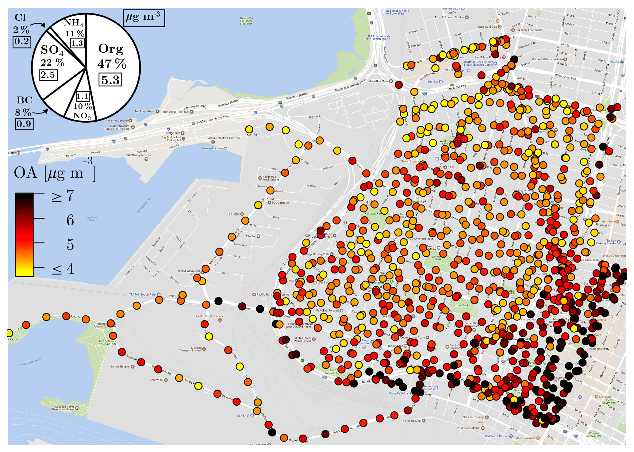
Figure 2Median organic aerosol concentration at each magnet. The pie chart shows the median contribution of AMS-measured non-refractory (organics: Org, sulfate: , nitrate: , ammonium: , chloride: Cl−) and aethalometer-measured black carbon (BC) to the total PM1. Boxed values are absolute mass concentrations in µg m−3.
The lower panel of Fig. 3 shows the central tendency statistics (mean, median, and standard deviation) of the values assigned to magnets in each area. The data are positively skewed in all polygons; i.e., the mean is higher than the median. Ambient measurements typically exhibit a positively skewed distribution under the influence of local emission events (Apte et al., 2017; Brantley et al., 2014; Seinfeld and Pandis, 2006; Van den Bossche et al., 2015). Hence, the median is chosen over the mean as a central tendency statistic to discuss the OA spatial patterns. The results shown in this figure are reinforced with statistical confidence by using bootstrap resampling (Fig. S5). We determined a precision of 0.5 µg m−3 in the median OA. Spatial differences larger than this precision are considered statistically significant.
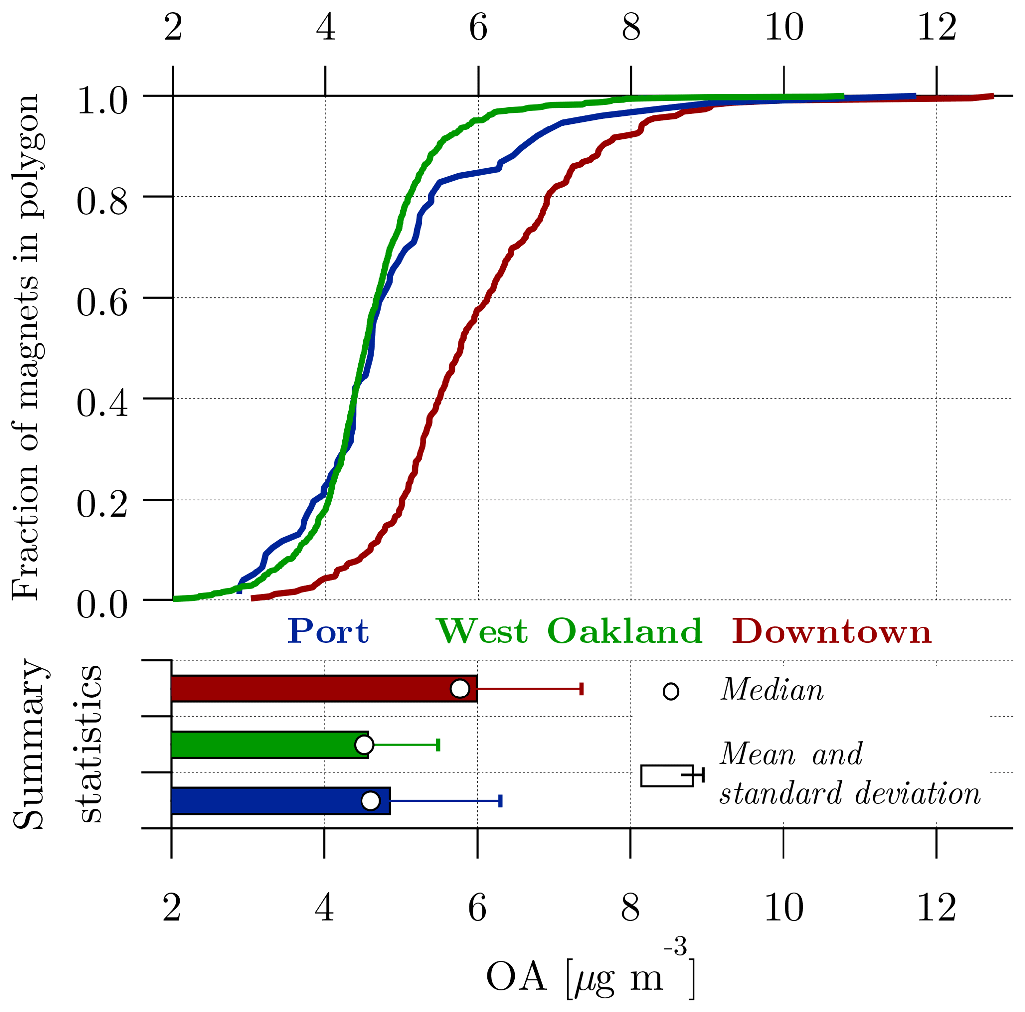
Figure 3Cumulative distributions, mean, and median of OA concentrations in Port, West Oakland, and downtown.
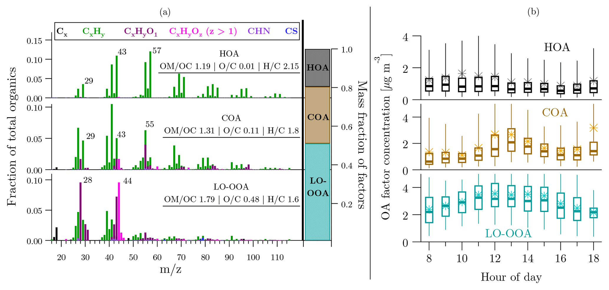
Figure 4(a) Mass spectra, elemental ratios, and average mass fraction of factors obtained from PMF analysis of all AMS spectra. (b) Box plot of diurnal profiles of factors: rectangles enclose the first through third quartiles of data. Horizontal bars are medians. Asterisk markers are means. Whiskers are the 5th and 95th percentiles.
Downtown has a median OA concentration of 5.7 µg m−3, which is 27 % higher than West Oakland and port. Almost the entire downtown CDF curve is ∼1.5 µg m−3 greater than the West Oakland and port curves, indicating that all parts of downtown have higher OA concentrations than the rest of Oakland. Port and West Oakland have similar OA concentrations, as evidenced by their nearly superimposed CDFs and similar medians (4.6±0.05 µg m−3). However, port measurements have more positive skewness than West Oakland; port has a larger fraction of magnets with high OA concentrations than West Oakland. This suggests that the OA concentrations in port are more influenced by local emission events. As mentioned earlier, port has high drayage truck activity, which likely explains this skewness. Results from bootstrapping support this explanation (Fig. S5). Port data have a higher mean (4.9 µg m−3) with a wider 95 % confidence interval (0.7 µg m−3) about this mean compared to West Oakland (mean: 4.6 µg m−3; 95 % confidence interval about the mean: 0.2 µg m−3).
3.2 OA factors
We identified three OA factors with distinct mass spectra using positive matrix factorization (PMF) of AMS data: hydrocarbon-like OA (HOA), cooking OA (COA), and less-oxidized oxygenated OA (LO-OOA). These factor profiles are shown in Fig. 4. Distinct features of each factor mass spectrum (e.g., signals at particular m∕z and elemental O ∕ C ratios) and the diurnal patterns in their time series are used to characterize these factors. We use the same nomenclature for these factors as has been used commonly in the literature. For comparison, previously reported mass spectra of these factors are shown in Fig. S9.
3.2.1 HOA
The HOA factor has an elevated signal at the series of CnH2n+1 (e.g., at m∕z 57) and CnH2n−1 (e.g., at m∕z 41). Previous studies have identified this factor as a marker of fresh vehicular emissions based on its reduced state (O ∕ C = 0.01) and its diurnal pattern (Mohr et al., 2012; Zhang et al., 2011). HOA time series are highly positively skewed (average of hourly mean ∕ median = 1.6) even during nonpeak periods, which indicates the influence of local HOA plumes.
3.2.2 COA
The COA factor has a distinct signal at m∕z 55 ( and C3H3O+). Previous studies have identified this factor as a marker of cooking emissions based on its reduced state (O ∕ C = 0.11) and its diurnal pattern (Mohr et al., 2009, 2012; Zhang et al., 2011). Similar to HOA, COA time series are also highly positively skewed (average of hourly mean ∕ median = 1.53), indicating the influence of local COA plumes.
3.2.3 LO-OOA
Compared to the HOA and COA factors, this factor is relatively more oxygenated with a distinct peak at m∕z 44 in its mass spectrum. Secondary OA contains oxygen-containing groups (e.g., carboxylic acids, alcohols, and carbonyls). These groups, upon ionization in the AMS, contribute to the m∕z 44 (COO+) signal. Generally, based on an increasing extent of atmospheric processing, two classes of oxygenated OA are identified by signals at m∕z 43 and 44: less- and more-oxidized oxygenated OA (Xu et al., 2015). Of these two, LO-OOA is relatively less oxygenated, bears similarity to semi-volatile OOA (SV-OOA) in the two-dimensional volatility basis set (Donahue et al., 2012), and is considered “fresh SOA” formed by the gas-phase oxidation of organic precursors emitted nearby (Hayes et al., 2013). LO-OOA is thus found to be strongly correlated with particulate .
Having made no thermodenuded measurements of OA volatility, we identify the third oxygenated factor in our PMF solution as LO-OOA because (a) the mass spectrum and elemental ratios are similar to those reported for LO-OOA (and SV-OOA) elsewhere (Fig. S9), and (b) this factor is correlated with the AMS-measured signal (Fig. S10). The diurnal pattern of the LO-OOA factor has a more normal distribution about midday. Additionally, the LO-OOA time series exhibit less positive skewness (average of hourly mean ∕ median = 1.07) compared to COA and HOA. Compared to the two primary factors, LO-OOA in Oakland has less spatial variability.
3.2.4 Contribution of OA factors
Average contributions of COA, HOA, and LO-OOA to total OA are shown in Fig. 4. COA and HOA collectively contribute ∼45 % of the total OA mass. This fraction of primary contributions to OA is higher than that reported for typical urban OA in prior studies (Crippa et al., 2013b; Zhang et al., 2007). Through mobile measurements in Pittsburgh, PA, Gu et al. (2018) find that ∼25 %–30 % of the annual average OA mass is primary. The relatively high contributions of primary OA suggest that OA in Oakland is more strongly influenced by local emissions than other locations.
Previous AMS-PMF studies have reported the presence of both LO-OOA and MO-OOA factors in ambient OA. The absence of an MO-OOA factor in Oakland can be explained by the hypothesis that air masses arriving in Oakland are oceanic. These air masses are expected to contain very low OA concentrations, even though most of this OA is highly oxidized MO-OOA (Hildebrandt et al., 2010). The MO-OOA in these oceanic air parcels would be rapidly overwhelmed by urban emissions as the air parcels are advected over San Francisco and Oakland, resulting in the apparent absence of an MO-OOA factor in Oakland. This hypothesis of predominantly oceanic air masses is confirmed by the wind rose diagrams in Fig. S17. Predominant winds measured at the Oakland anemometer during periods of mobile sampling are from between the northwest and southwest with typical wind speeds of ∼10 km h−1. This means that Oakland falls roughly 60 min downwind from the Pacific Ocean. Emissions from the metropolitan SF area are likely advected to Oakland, although the timescale of this advection is <60 min. On this timescale, LO-OOA formation from the SF emissions could be expected, but MO-OOA formation in amounts such that it would be detectable after mixing with the local emissions in Oakland is not expected (Decarlo et al., 2010; Jimenez et al., 2009). The LO-OOA factor profile shown in Fig. 4 has a minor contribution from methanesulfonic acid (m∕z 79), which was previously found to be an indicator of the marine origin of air parcels (Crippa et al., 2013a). This finding confirms that the air masses arriving in Oakland are predominantly oceanic.
3.2.5 Quality of PMF solution
PMF decomposes measured OA concentrations using a linear combination of contributions from static factors. The amount of observed mass that cannot be explained by the reconstructed factor contributions is binned into residual mass. Residuals of factorization are shown in Fig. S11. The ratio of scaled residuals, Q, to the total degrees of freedom of the fitted data, Qexp, would be ≈1 in a perfect factorization (Ulbrich et al., 2009). PMF numerically approaches a convergence using different initial starting points (fpeak) in the rotational domain about zero (Paatero and Tapper, 1994). Values of Q∕Qexp for different values of fpeak are shown in Fig. S14, along with the factor mass fractions for each solution. Our three-factor PMF solution is very stable () and the factor mass fractions do not change with varying fpeak.
A four-factor solution was also examined (Fig. S12). While the mass spectra and fractional contributions of both HOA and COA remain unchanged from the three-factor solution, the LO-OOA factor from the three-factor solution was further deconvolved into a more oxygenated MO-OOA factor and a fourth less oxygenated factor that bore no similarity to the typical LO-OOA factor spectra reported in the literature. We discarded this four-factor solution because (a) given that fresh OA factors (HOA and COA) and OOA factors form a continuum of atmospheric oxygenation, we do not expect the presence of the fresh OA and MO-OOA factors while an LO-OOA factor is absent, (b) we did not find a strong PMF-independent tracer correlation (e.g., with AMS-measured particulate or ) for the MO-OOA and the fourth factor, and (c) going from three-factor to four-factor solution, there was only a 5 % reduction in Q∕Qexp, suggesting not only diminishing returns with a number of factors less than three, but simply an artificial splitting of the optimal solution, which would result in an overinterpretation of the PMF results (Ulbrich et al., 2009). This artificial splitting is also evidenced and discussed later using elemental analysis in Sect. 3.5.
3.3 Spatial and temporal variability of OA factors
In this section, we further analyze the spatial and temporal patterns of OA and its factors. All times are presented in local time (Pacific Daylight Time, UTC minus 7 h). We begin by examining the primary–secondary split of OA and how this split varies across space and time. Understanding variability in the primary fraction of OA is important because we know from recent findings that in close proximity to sources such as highways (Saha et al., 2018b) and restaurants (Robinson et al., 2018), there is high amount of primary OA mass in Aitken-mode particles (Ye et al., 2018) and the particle population is externally mixed. Atmospheric processing of these emissions (e.g., increasing SOA fraction, coagulation with background particles) makes the particle size distributions more unimodal and internally mixed in the accumulation mode (Ye et al., 2018). This primary–secondary split may have important health exposure implications because Aitken-mode particles have longer retention times once they penetrate lung tissue (Ferin et al., 1992; Oberdörster, 2000; Stölzel et al., 2007).
Overall, the OA mass in Oakland is split into primary and secondary factors roughly evenly (Fig. 4): two primary factors (COA + HOA) collectively contribute ∼45 %, while the rest is secondary (LO-OOA). However, the primary–secondary split at each magnet is spatially and temporally variable. To identify areas with elevated levels of primary emissions, we normalized the sum of COA and HOA to the total OA concentration at each magnet, which results in a primary fraction of the OA at the magnet. In Fig. 5a, we show a map of the primary fraction of OA at each magnet in the domain. It is evident that the OA in parts of downtown has a higher than 50 % contribution from primary sources. Other areas exhibiting higher fractions of primary sources are the highways. In the more residential areas (West Oakland), LO-OOA contributes ∼55 % of the OA (Fig. 5d). Through bootstrap resampling, a precision of ∼1.5 % was determined for the primary fraction of OA (Fig. S6).
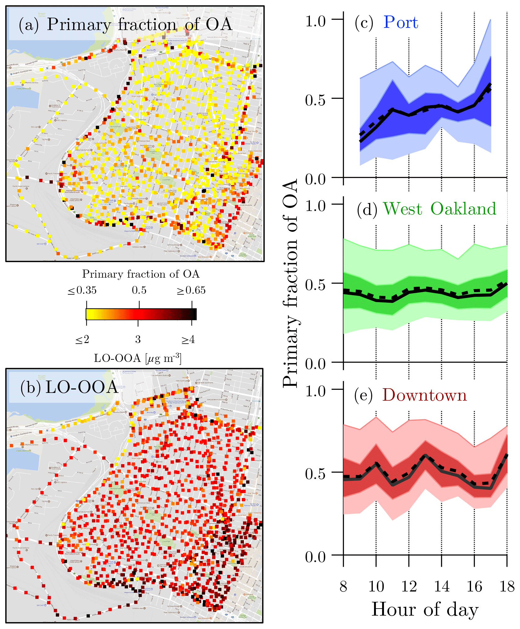
Figure 5(a) Median primary fraction of OA at each magnet. Primary fraction is defined as the ratio of COA + HOA to the total OA at each magnet. (b) Median LO-OOA concentration at each magnet. Also shown are diurnal profiles of the primary OA fraction in (c) port, (d) West Oakland, and (e) downtown. Solid and dashed lines are hourly medians and means, respectively. Darkly shaded areas enclose the first and third quartiles of data. Lightly shaded areas enclose the 5th through 95th percentiles of data.
Figure 5b shows a map of the LO-OOA mass concentrations. While LO-OOA has a smoother spatial pattern than primary OA, downtown exhibits higher LO-OOA concentrations. Individual maps of COA and HOA are shown in Fig. S18. Figure 5 also shows the diurnal profiles of the primary contributions to OA in port, West Oakland, and downtown. The primary OA contributions in port and downtown are more temporally variable than in West Oakland. Generally, primary OA contributions in port have a positive trend (from ∼25 % to 60 %) with increasing hour of day, with peaks occurring at ∼11:00 and 18:00 LT. This is likely due to an increasing volume of trucks as the day progresses. By contrast, primary contributions in downtown are consistently around 50 % of the total OA, with peaks during high traffic periods and lunchtime. Primary contributions in West Oakland are consistently around 45 %, with no distinct peaks.
Figure 6 shows a scatter plot of COA versus HOA contributions to OA from the entire campaign, which is meant to show the diurnal variation of primary OA sources. During the morning rush hour, concentrations of COA and HOA are roughly equal. Primary OA concentrations start transitioning towards COA dominance at ∼ 11:00, which coincides with the typical time restaurant kitchens would be expected to begin activity. By ∼14:00 LT, COA dominates the primary OA mass.
In Fig. 7, we show the spatial and temporal patterns of total OA as well as the three OA factors by resolving them by area (port, West Oakland, and downtown) and time of day: morning (08:00 to 11:00 LT), midday (11:00 to 14:00 LT), and afternoon (14:00 to 18:00 LT). To aid discussion with statistical confidence, we refer the reader to Fig. S7, which shows the 95 % confidence intervals of these results obtained from bootstrap resampling. As described earlier, we consider the 95 % confidence interval of the bootstrapped median as an indicator of precision; i.e., spatial differences larger than this precision are deemed statistically significant. Overall, OA factors have a ∼0.25 µg m−3 precision. This precision agrees with that determined in an independent dataset acquired in Pittsburgh, PA (Gu et al., 2018).
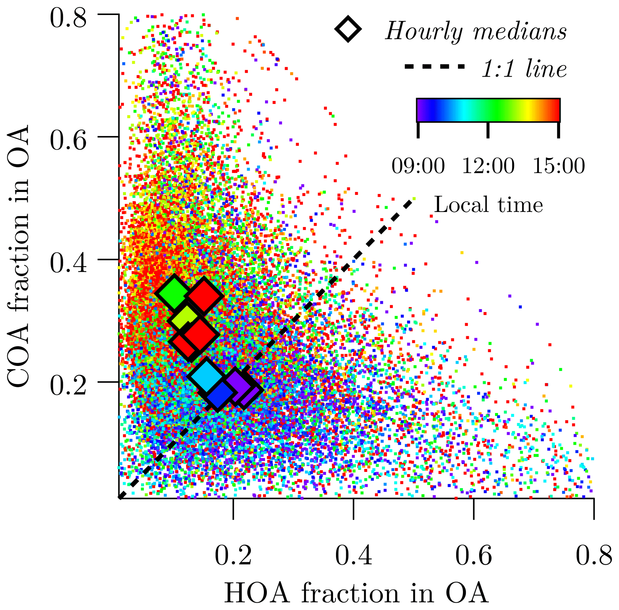
Figure 6Diurnal shift of the source of primary OA from morning rush hour traffic to midday cooking activities. Dots show individual measurements and diamonds show hourly medians over the entire sampling campaign.
3.3.1 OA
During the morning period (08:00 to 11:00 LT), the median OA concentration in downtown is 40 % (∼ 1.7 µg m−3) higher than in West Oakland and port. Median OA in port and West Oakland are similar (within precision). On average, the median OA concentration in the entire domain is 16 % (∼0.8 µg m−3) higher during midday (11:00 to 14:00 LT) compared to the morning period. The median OA concentration in downtown is 40 % (∼1.9 µg m−3) higher than in West Oakland and 21 % higher than in port. During the afternoon (14:00 to 18:00 LT), the median OA concentration over the entire domain is 20 % (∼1.2 µg m−3) lower than the midday period. Median OA concentration in downtown is similar to West Oakland (4.6±0.14 µg m−3) and 17 % higher than in port. Overall, total OA concentrations in downtown are consistently higher than port and West Oakland during morning, midday, and afternoon periods.

Figure 7Cumulative distribution functions of total OA and the three factors identified in this study resolved by area (port, West Oakland, and downtown) and local time (LT) of day: morning (08:00 to 11:00), midday (11:00 to 14:00 LT), and afternoon (14:00 to 18:00 LT). The colored box around each set of CDFs indicates the period of the day those data represent.
3.3.2 HOA
During the morning period, the median HOA concentration in downtown is 52 % (∼0.5 µg m−3) higher than in West Oakland. The median HOA concentration in West Oakland, in turn, is 32 % higher than port. There is no net increase in median HOA concentration in the entire sampling domain from morning to midday. However, from morning to midday, the median HOA is reduced by 16 % and 20 % in downtown and West Oakland, respectively, while that in port increases by 64 % (∼0.4 µg m−3). As a result, during midday, the median HOA in downtown and in port are similar (1.1±0.01 µg m−3) and higher than that of West Oakland by 58 % (∼0.4 µg m−3). On average, the median HOA concentration in the entire domain is ∼0.2 µg m−3 lower during the afternoon compared to the midday and morning periods. Median HOA concentrations in the three polygons are all similar at 0.8±0.06 µg m−3, with port being highest.
Overall, HOA is highest in downtown in the morning, despite the fact that all of Oakland has roughly equal proximity to highways. While we do not have detailed traffic data for Oakland, it is reasonable to assume that downtown receives a large influx of commuters during the morning rush hour and thus would be expected to have the highest HOA concentrations. Downtown also has a higher road length density compared to West Oakland and port and, as a result, can accommodate a larger traffic volume per km2. Further, poor ventilation of vehicle emissions in downtown can also contribute to higher HOA levels (Yuan et al., 2014). During midday and afternoon, however, port has similar or higher HOA than downtown. This is expected for two reasons: (a) the commuters contributing to high HOA in downtown during the morning hours are working (and their cars parked) during midday, and (b) there is a high amount of drayage truck activity in port. There is some evidence from fuel sales data that truck activity at the port is higher in the afternoon than the morning. One of the measures implemented to reduce port emissions was to keep shipping logistics gates open in the evening to dilute the daytime congestion of drayage trucks (Port of Oakland, 2016), which may contribute to trucks at the port not following the typical rush hour traffic patterns of commuters. West Oakland has the lowest HOA concentrations at all times of day, as would be expected for a largely residential area.
3.3.3 COA
The median COA concentration in downtown is 55 % (∼0.5 µg m−3) higher than in West Oakland and 109 % higher than in port during the morning period. Further, COA concentrations in downtown exhibit a larger positive skew (mean ∕ median = 1.5) relative to both West Oakland and port (mean ∕ median = 1.15). On average, the median COA concentration in the entire domain is ∼0.8 µg m−3 higher during midday compared to the morning period. The median COA concentration in downtown is 27 % higher than in West Oakland and port during midday. On average, the median COA concentration in the entire domain is ∼0.3 µg m−3 lower during the afternoon compared to the midday period. The median COA concentration in downtown is 11 % and 26 % higher than in West Oakland and port, respectively.
Overall, COA is consistently highest in downtown, which is not surprising given the large number of restaurants. The spatial distribution of COA in West Oakland and port is uniformly low in the morning, as demonstrated by the steepness of the distribution functions in Fig. 7. During midday and late afternoon, however, COA levels in both these areas are higher than in the morning. It is not clear why COA in port is higher than West Oakland during midday. It should be noted, however, that due to the considerably low road length density in port, the number of magnets in port is only ∼10 % of those in West Oakland. As a result, even a few cooking sources in port (most likely food trucks) could cause the spatially aggregated values for port to appear higher than West Oakland. Overall, port has the lowest COA concentrations, which is expected given the land use in that area.
3.3.4 LO-OOA
The median LO-OOA concentration in downtown is 36 % (∼0.9 µg m−3) and 17 % higher than in West Oakland and port, respectively, during the morning period. On average, the median LO-OOA concentration in the entire domain is 15 % (∼0.5 µg m−3) higher during midday than the morning period. During midday, the median LO-OOA concentration in downtown is 18 % (∼0.6 µg m−3) higher than in West Oakland and 8 % higher than in port. On average, the median LO-OOA concentration in the entire domain is 20 % (∼0.5 µg m−3) lower in the afternoon compared to the midday period. Median LO-OOA concentrations in all three areas are similar (2.9±0.2 µg m−3), with downtown being the highest and port being the lowest.
LO-OOA concentrations are consistently higher in downtown compared to port and West Oakland. This finding is unexpected because LO-OOA is secondary; the null hypothesis for secondary species is that concentrations would be spatially uniform. Multiple lines of evidence contribute to the conclusion that LO-OOA is indeed higher in downtown than the port and West Oakland. First, as shown in Figs. 7 and S7, morning-time LO-OOA concentrations are 0.9 and 0.5 µg m−3 higher in downtown than in port and West Oakland. Given our determined precision of 0.25 µg m−3 in OA factors, these spatial differences are significant. As shown in Fig. S1, our sampling times are not temporally biased; therefore, higher LO-OOA downtown does not appear to be an artifact of our sampling strategy (e.g., downtown is not over-sampled at midday relative to West Oakland and port). Second, the LO-OOA CDFs in Fig. 7 are further substantiated by east–west transect drives performed during inter-polygon transits on different days of the campaign and shown in Fig. 8. These transects show that there is a general trend of increasing LO-OOA concentrations between the port and downtown. Third, the enhanced LO-OOA downtown echoes similar measurements made independently in Pittsburgh, where fresh SOA is also enhanced in the downtown area (Gu et al., 2018).
The increasing concentrations of LO-OOA with increasing inland distance (Fig. 8) can be explained by the predominant westerly winds (Fig. S17). At the typical wind speed of ∼15 km h−1, downtown is 10–15 min downwind from the port. The additional processing of OA in this time can result in higher LO-OOA in downtown. However, we also observe that the spatial pattern of LO-OOA changes diurnally, with a stronger spatial gradient in the morning than the afternoon (Fig. 7). This suggests that the local photochemical microenvironment may also contribute to the observed LO-OOA spatial pattern.
The enhanced photochemical production of SOA could be due to several factors. First, the pool of reactive SOA precursor vapors is likely enhanced in downtown relative to other areas. We show above in Fig. 7 that HOA is highest in downtown. HOA is co-emitted with volatile and intermediate-volatility organic compounds that efficiently generate SOA upon photochemical oxidation (Gordon et al., 2013; Robinson et al., 2007; Zhao et al., 2015).
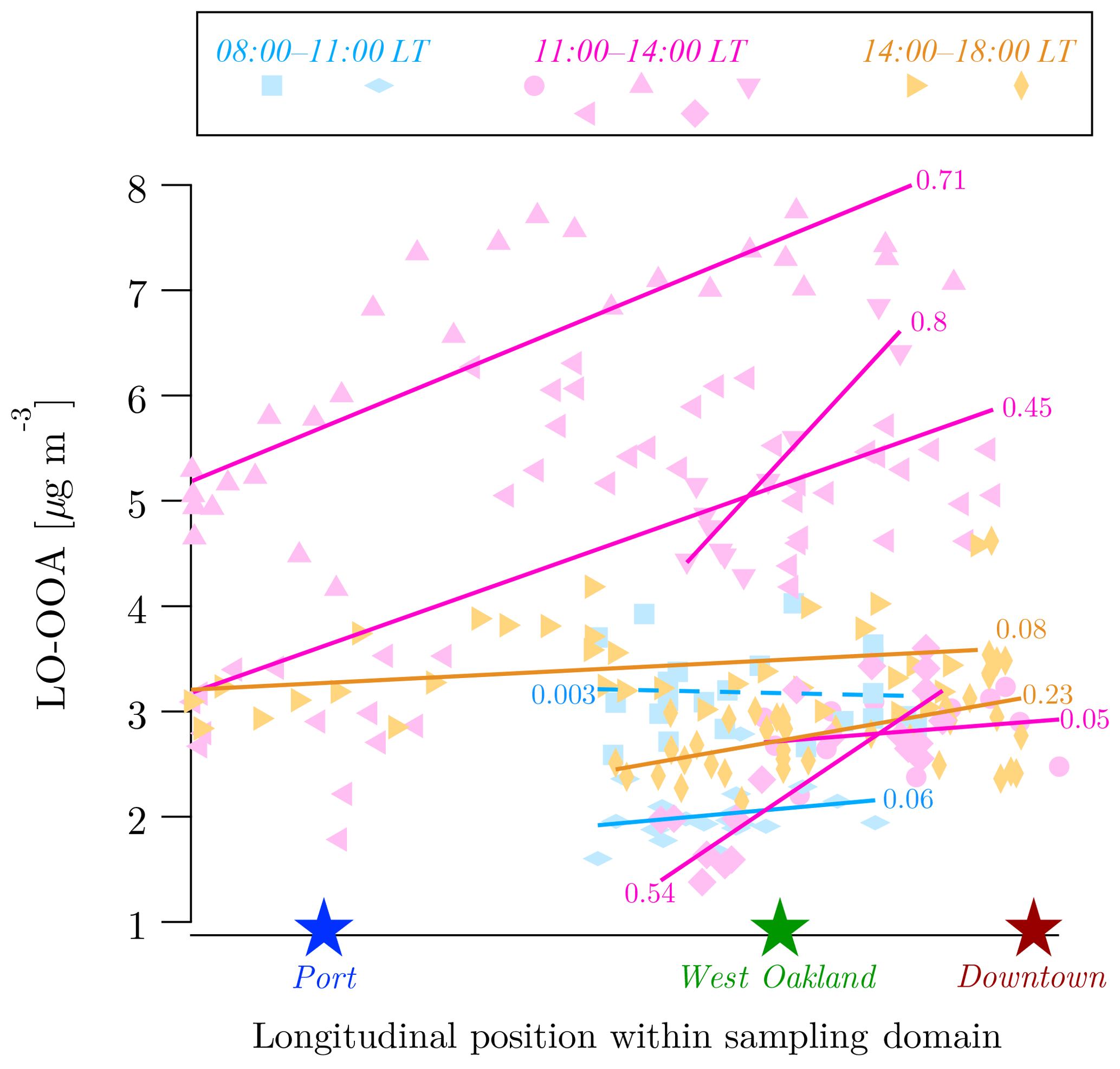
Figure 8Spatial variations in measured LO-OOA on select intra-polygon transit drives on different days, colored by three different diurnal local time (LT) periods. Drives that reasonably spanned the longitudinal extent of the sampling domain with minimal latitudinal displacement were picked for this plot. Markers are individual LO-OOA samples and lines are fits for each transect drive. Fits that have a positive slope with proximity to downtown are shown as solid lines. The only fit that has a negative slope is shown as a dashed line. R2 of fits are shown next to fits. Approximate locations of port, West Oakland, and downtown are shown as references to better visualize longitudinal positions of data.
Second, concentrations of the hydroxyl (OH) radical may also be higher downtown. The OH radical is the dominant daytime oxidizing agent, especially for reduced compounds emitted from motor vehicles. It has been shown that in urban, polluted environments (street canyons), high NOx emissions from vehicles render increased levels of nitrous acid (HONO), which in turn results in increased local oxidation capacity (Villena et al., 2011; Yun et al., 2017) due to the rapid photolysis of HONO to OH (Finlayson-Pitts and Pitts, 2000; Stutz et al., 2000; Zhong et al., 2017).
A third factor may also contribute to higher precursor concentrations and therefore additional LO-OOA in downtown. The presence of tall buildings in downtown can create higher surface roughness, which in turn can reduce pollutant dispersion and promote internal recirculation (Zhong et al., 2017). This possibility is further examined in Fig. S19, which shows building heights in downtown. Downtown has relatively taller buildings that collectively act as a wall parallel to the Interstate 980 highway upwind. The air masses in downtown may experience stagnation and poor ventilation relative to West Oakland and port. This, in turn, can increase the reaction time, thereby allowing for more local LO-OOA formation.
The combined impact of vehicle emissions on OH (via HONO) and gas-phase precursor concentrations in downtown would be expected to be largest in the morning, since these are co-emitted with HOA. Indeed, the largest enhancement of LO-OOA in downtown occurs in the morning hours at the same time as the largest enhancement of HOA. From morning to midday, LO-OOA concentrations become more spatially uniform; median LO-OOA concentrations in West Oakland and port increase by 23 % (0.6 µg m−3) and 16 % (0.5 µg m−3), respectively, while downtown only increases by 7 % (0.25 µg mm−3). This suggests that while downtown has high photochemical activity in the morning, the entire sampling domain transitions towards a more uniform photochemical state by midday.
We further investigated the enhanced photochemical activity in downtown by analyzing mobile measurements of particulate sulfate (). is formed upon the reaction of gas-phase SO2 with OH (Miyakawa et al., 2007), which can be enhanced in polluted environments due to the catalytic involvement of black carbon particles (Novakov et al., 1974). Figure S8 shows that concentrations in downtown are higher (∼8 %) than port and West Oakland, a trend similar to that observed for LO-OOA concentrations.
Ships associated with the port are the major source of SO2 in Oakland (Tao et al., 2013). While ship SO2 emissions have significantly decreased in recent years, ships remain the dominant SO2 source in our sampling domain, and there seem to be no local sources of SO2 or particulate in downtown. Thus, elevated concentrations of secondary sulfate in downtown would therefore support the hypothesis that OH concentrations are also higher in downtown, giving rise to local variations in the formation rate.
3.4 Spatial patterns of gasoline and diesel vehicle emissions
In this subsection, we compare the influence of emissions from diesel trucks against that from gasoline-powered vehicles. We do this by comparing concentrations and ratios of OA, HOA, BC, and CO. Traditionally, diesel vehicles have significantly higher emissions of HOA and BC than gasoline vehicles (Ban-Weiss et al., 2008), whereas gasoline vehicles have higher CO emissions than diesel vehicles (May et al., 2014). Vehicle emission standards are regularly tightened, so emissions are lower for newer vehicles. However, emission reductions are not equal for all species, so the ratios of different emitted pollutants vary with both vehicle age and fuel type. Thus, the specific emissions and emission ratios from the vehicle fleet in a city, or a portion of the city, depend on both the gasoline–diesel split and the age distribution of gasoline and diesel vehicles.
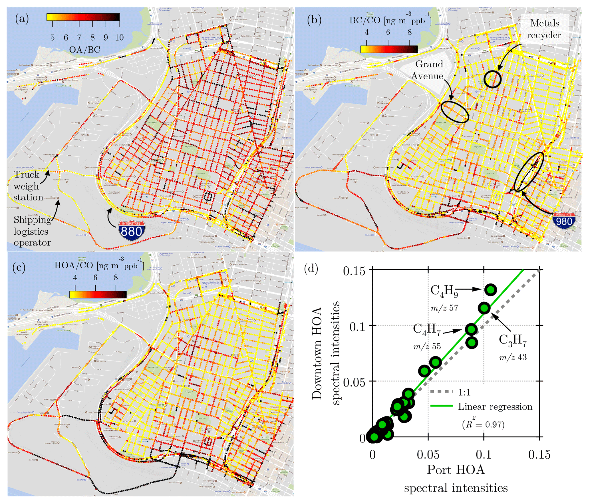
Figure 9Fine-scale maps of (a) OA ∕ BC (unitless), (b) BC ∕ CO, and (c) HOA ∕ CO. Panel (d) shows similarity between the HOA factors identified by factorization of port-only and downtown-only OA data. The two spectra are dominated by hydrocarbons (CxHy) and are highly similar to each other.
Based on typical emissions from gasoline and diesel vehicles, we would expect that (a) all areas with heavy traffic should have elevated concentrations of OA, HOA, BC, and CO, and (b) diesel-dominated areas will have higher BC ∕ CO, higher HOA ∕ CO, and lower OA ∕ BC ratios than gasoline-dominated or background locations. The specific concentration ratios in different areas will be a function of the vehicle fleet in that area and the contribution of fresh emissions versus background. One potential drawback of using concentration ratios to identify gasoline- versus diesel-dominated areas is that emission ratios from cars are becoming more “diesel-like” (May et al., 2014; Saliba et al., 2017), which complicates the analysis for newer vehicle fleets.
Figure 9a–c show spatially resolved OA ∕ BC, BC ∕ CO, and HOA ∕ BC ratios. Because measurements were made at different sampling frequencies, we generate the ratios by first converting the measurements to a synthetic 1 Hz time base as described earlier. All three ratios show an influence of diesel trucks (lower OA ∕ BC, higher BC ∕ CO, and HOA ∕ BC) at the port, on Interstates 880 and 980, and on truck routes that connect I-880 to the port. The absolute concentrations of BC are also elevated in these areas (Fig. S20). Bootstrap resampling the BC dataset shows that the measurements (especially in port) have a considerable positive skew (Fig. S21). The ratio of mean to median BC in port is higher (1.5) than both West Oakland and downtown (1.2). Because BC concentrations are largely influenced by local sources (diesel trucks), the large amount of drayage trucks in port likely causes the mean BC to be ∼8 % higher than downtown, even though the median BC in downtown is ∼7 % higher than port.
All three ratios suggest less diesel influence in West Oakland and downtown than in port. BC ∕ CO ratios in the port are generally 6–8 ng m−3 ppb−1, whereas much of West Oakland and downtown have BC ∕ CO ∼4 ng m−3 ppb−1. Some hot spots of BC ∕ CO appear in industrial parts of West Oakland, including (a) an area near a metals recycling facility in West Oakland highlighted by Apte et al. (2017) as a location with high diesel traffic and (b) a part of Grand Avenue, which is also a truck route. A hot spot of BC ∕ CO also appears on and downwind of I-980 in downtown.
The HOA ∕ CO ratio paints a similar but not identical picture to the BC ∕ CO ratio. West Oakland and downtown have lower HOA ∕ CO than the port, suggesting less diesel truck influence. However, downtown has higher HOA ∕ CO than West Oakland. Since gasoline cars appear to be the major traffic source in West Oakland and downtown, we would expect a similar HOA ∕ CO ratio in these areas. However, several factors may contribute to the higher HOA ∕ CO in downtown: (a) the downtown and West Oakland fleets are likely not identical (e.g., more diesel buses in downtown), (b) there are differences in driving mode, with more stop-and-go driving in downtown than West Oakland, and (c) there is a larger contribution of background CO to the total measured CO in West Oakland.
The overall picture painted by Fig. 9a–c is that the port is more impacted by diesel vehicle emissions than downtown and West Oakland. Downtown has high HOA (Fig. S18) because of high traffic volumes, but this area seems to be dominated by gasoline vehicles with a smaller diesel contribution. The large diesel influence at the port persists in spite of recent aggressive efforts to upgrade the drayage truck fleet so that the majority (99 %) of drayage trucks now have diesel particulate filters (Preble et al., 2015). As shown by Dallmann et al. (2011) and Preble et al. (2015), overall BC emissions from the port truck fleet fell by ∼75 % between 2010 and 2013, suggesting that HOA and BC concentrations at the port were higher in the past. Further reductions in BC and HOA at the port could be achieved by addressing high emitters; measurements by Preble et al. (2018) in 2015 showed that 7 % of the drayage truck fleet at the port accounted for 65 % of the total emitted BC because the diesel particulate filters on these trucks were failing.
Since the vehicle fleet appears to be significantly different between downtown and port, we attempted to derive separate HOA factors for these two areas as a means to directly quantify gasoline versus diesel emissions using the AMS. We isolated port OA data from downtown OA data and factorized them separately using PMF. The HOA factors identified for port and downtown are nearly identical (R2=0.97; Fig. 9d). This is likely due to a combination of similar emissions (Worton et al., 2014; X. Li et al., 2016) and excessive fragmentation upon ionization in the AMS. The similarity in the port and downtown HOA factors makes it essentially impossible to distinguish HOA emitted by diesel trucks from HOA emitted by gasoline cars.
3.5 Elemental analysis of bulk and factor OA
In this section, we investigate the measured elemental ratios (H ∕ C and O ∕ C) of OA using a Van Krevelen (VK) diagram. Figure 10 shows all bulk OA data from this study (gray dots). Only 21 % of the bulk data fall inside the typical ambient range of OOA measurements (Ng et al., 2011), while the remaining data are on the less oxygenated side of this range. This indicates a dominant presence of highly reduced, primary OA in Oakland. This finding contrasts with the measurements made in other urban areas. For instance, almost all of the bulk OA measurements made in Pasadena, CA, were either inside or below (i.e., more oxygenated than) this ambient OOA region (Ortega et al., 2016). This finding is consistent with the large contribution of primary OA in Oakland (Figs. 4 and 5) and can be partially explained by the overall spatial proximity of ≤1 km of all points inside the domain to the nearest highway (Apte et al., 2017). Primary emissions are thus of more importance in Oakland than other urban areas.
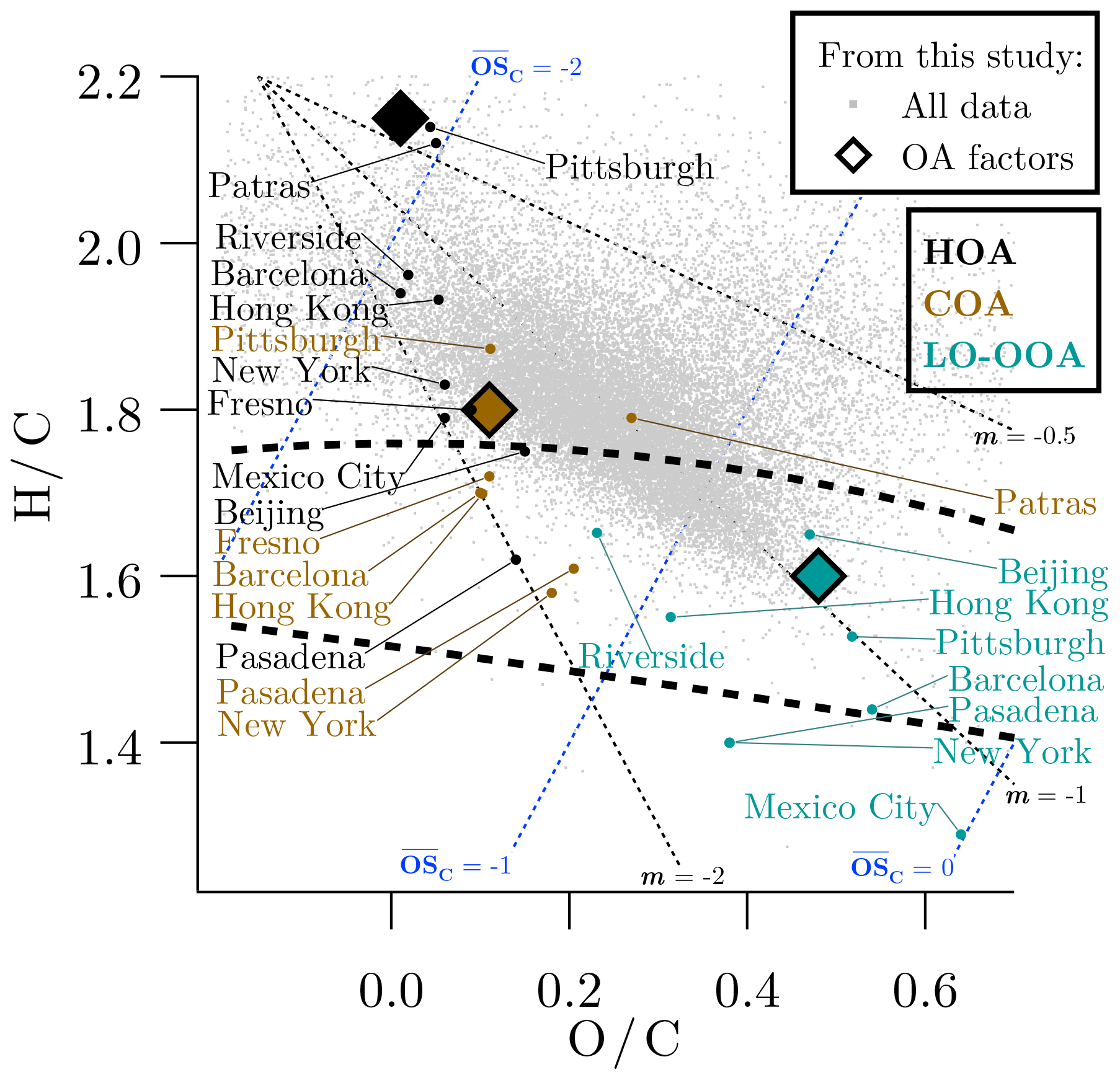
Figure 10The Van Krevelen plane. Gray points represent all OA measurements in this study. Diamonds represent OA factors identified in this study. For reference, the placement of OA factors from other ambient measurements is shown: Pittsburgh (Gu et al., 2018), Patras, Greece (Kaltsonoudis et al., 2017), Riverside, CA (Docherty et al., 2011), Barcelona (Mohr et al., 2012), Hong Kong (Lee et al., 2015), New York, NY (Sun et al., 2011), Fresno, CA (Ge et al., 2012), Mexico City (Decarlo et al., 2010), Beijing (Hu et al., 2016), and Pasadena, CA (Hayes et al., 2013). Different oxygenation pathways are shown by the black dotted lines. Dotted blue lines are isopleths for average carbon oxidation states (). The region of ambient oxygenated OA measurements, as reported by Ng et al. (2011), is shown between the dashed curves.
Figure 10 also shows that the cluster of bulk OA data from this study aligns with the −1 slope line (slope of linear fit , not shown; Pearson's R=0.62). Previous studies have used VK slopes to determine if the processing of ambient OA is dominated by chemical (e.g., oxygenation) or physical (e.g., external mixing of air masses) mechanisms. By isolating the chemical processing of Pasadena OA in an oxidation flow reactor, Ortega et al. (2016) showed that chemical processing shifts OA on the VK plane along a shallow slope of . A similar slope was observed by Liu et al. (2018) by chemical processing of Beijing OA in an oxidation flow reactor. Similarly, Presto et al. (2014) measured a slope of for the oxidation of fresh gasoline and diesel exhaust in a smog chamber. By comparing OA measurements in Riverside, CA, with those in Pasadena, Hayes et al. (2013) hypothesized that the HOA-to-LO-OOA transformation in Riverside occurred with a steeper VK slope () due to the physical mixing of highly reduced (Canagaratna et al., 2015; Kroll et al., 2011), HOA-rich air masses with OOA-rich air masses in Riverside.
Figure 10 also plots the HOA, COA, and LO-OOA factors identified in this study on the VK plane. For reference, similar factors are shown from ambient measurements reported in prior publications. As expected, reduced factors corresponding to primary emissions (HOA and COA) occur closer to the top left corner of the VK plane, while the LO-OOA factors occur closer to the bottom right corner. With the exception of Pittsburgh and Patras, HOA in Oakland is more chemically reduced () compared to HOA in other locations (average ). That the composition of HOA in Oakland is more reduced, and that the overall slope for all OA measurements in Oakland is , suggests that external mixing of highly reduced, HOA-rich air masses with OOA-rich air masses is an important processing mechanism in Oakland. This is also consistent with the recent findings of Ye et al. (2018) via single-particle mass spectrometry in Pittsburgh, PA; the particle mixing state shifts from internal to external with approximately kilometer-scale proximity to urban sources. It is also worth noting in Fig. 10 that the HOA measurements that are more chemically reduced (Oakland, Pittsburgh, and Patras) were performed in the past 5 years compared to the other measurements that were made earlier (∼10 years ago). This suggests a change in the chemical composition of vehicular emissions over the past decade.
Finally, this VK analysis also reinforces the choice of a three-factor PMF solution in this study. In Fig. S15, the three- and four-factor PMF solutions are compared on the VK plane, along with other reference data as already described in Fig. 10. The HOA and COA markers do not change their position on the VK plane between the three- and four-factor solutions. This is consistent with the robustness of HOA and COA mass fractions to the choice of PMF solutions, as described earlier and shown in Fig. S14. However, the LO-OOA factor in the three-factor solution is split into a highly oxygenated MO-OOA factor and a fourth unknown factor. We explained earlier that the four-factor solution is an artificial splitting of the three-factor solution. The placement of these factors on the VK planes is consistent with this explanation. The MO-OOA factor occurs in the bottom far-right corner, where there are no bulk OA data. The fourth OA factor coincides with the center of mass of the bulk OA data cluster, likely because the artificial splitting of the LO-OOA factor is done with the constraint of minimizing residuals (Q∕Qexp). Further, the LO-OOA, MO-OOA, and unknown factor all fall on the same m=1 dotted line. Thus, from a strictly mathematical standpoint, this solution offers no new information given that the MO-OOA and unknown factor average along the m=1 line to form the LO-OOA factor.
Having one of the largest shipping ports in the US, the air quality in Oakland has been historically impacted by shipping-related activities such as the presence of ships burning high-sulfur fuel and drayage trucks driving through the directly adjacent residential neighborhood (Fisher et al., 2006; Fujita et al., 2013). In the past decade, regulations on ship fuel usage have dramatically reduced emissions (Dallmann et al., 2011; Preble et al., 2015; Tao et al., 2013). Further, more than 70 % of the ships at the port now utilize shore power provision and thus do not idle their engines. It is thus reasonable to expect that the influence of ship emissions on the air quality in Oakland has been substantially reduced after the measurements of Tao et al. (2013). Enforced installation of diesel particulate filters on drayage trucks has also significantly reduced truck emissions at the port (Dallmann et al., 2011; Preble et al., 2015), although a recent finding by Preble et al. (2018) has raised concern about the exhaustion of these filters and the resultant increase in truck emissions.
In addition to the port, Oakland also has a central business district (“downtown”) that has activities such as domestic vehicular traffic and cooking, similar to other urban areas. Urban downtowns are also a prominent source of organic aerosol (Mohr et al., 2015), which makes up a dominant part of particulate matter (PM). Since the residential West Oakland neighborhood falls in the middle of the port and downtown, it is important from a health exposure perspective to determine the spatial variability of pollutants within the city and to determine which of these two source areas drive spatial variability in PM.
The objective of this study was to examine the spatial and temporal patterns in pollutants impacting the air quality in Oakland through mobile sampling in an instrumented van. Organic aerosol (OA) contributes the largest fraction (∼50 %) of PM1 mass. We find that primary emissions from cooking (COA) and vehicles (HOA) as well as secondary OA (LO-OOA) contribute to the spatial variation within Oakland. Key findings are the following.
-
Organic aerosol is the dominant component of PM1 (OA; ∼50 %), and its contribution is roughly twice that of sulfate (23 %). This finding is consistent with that of Tao et al. (2013), who also showed that the enforcement of low-sulfur fuel usage in ships has successfully reduced the amounts of particulate-phase in the local PM in Oakland.
-
In downtown, concentrations of primary OA are higher than secondary OA. The dominant source of these primary OA emissions shifts diurnally between cooking and vehicles: pre-10:00 LT fresh emissions are from vehicles, but cooking emissions contribute dominantly to OA after lunchtime.
-
While it is challenging to mathematically apportion traffic-emitted OA between drayage trucks and cars, we use ratios of OA and black carbon (BC; particulate matter typically emitted from diesel combustion in trucks) to CO and show that drayage truck emissions have an important effect on the concentrations of OA and BC at the port, especially when truck traffic typically peaks in the afternoon. However, cars seem to be the dominant source of traffic emissions in downtown and West Oakland.
-
Secondary OA (SOA) also exhibits spatial variability similar to primary OA. LO-OOA concentrations are higher in downtown, likely because a combination of various factors (poor ventilation of air masses in street canyons, higher emissions of SOA precursors, higher OH concentrations) results in downtown being a microenvironment with high photochemical activity.
-
The overall chemical composition of OA in Oakland is more chemically reduced relative to that reported in studies in several other locations. HOA in Oakland is particularly more reduced than other locations. This reflects the importance of primary emissions in Oakland. Further, by comparing measurements from other studies, we show that the chemical composition of HOA has likely become more reduced over the last decade. Lastly, external mixing of air masses with contrasting pollutant concentrations plays an important role in the processing of these chemically reduced emissions.
These findings have important implications for population exposure studies because urban downtowns tend to have a concentrated presence of workplaces, resulting in people being exposed to these elevated pollutant concentrations for ∼8 h (typical workday duration) every day. These findings are experimentally shown for Oakland as a case city, which has unique elements (oceanic winds mixing with urban emissions, presence of a major port) that likely have a unique influence on the intracity patterns in its air quality. However, Oakland also has elements that are fairly typical of urban areas (e.g., downtown with high cooking and vehicular emissions). The findings of this study are thus likely applicable to other urban areas as well because the pollutants we find contributing the most to OA variability, both of primary and secondary origin, are ubiquitous in other urban locations.
The supplement related to this article is available online at: https://doi.org/10.5194/acp-18-16325-2018-supplement.
RUS, ESR, and PG collected data. RUS performed data analysis with input from all coauthors on the interpretation of results. RUS and AAP wrote the paper with significant input from ALR. ALR, JSA, and AAP designed the research.
The authors declare that they have no conflict of interest.
This work has not been formally reviewed by the funding agencies. The views expressed in this document are solely those of the authors and do not necessarily reflect those of the funding agencies. EPA does not endorse any products or commercial services mentioned in this publication.
This research was funded by Environmental Defense Fund (EDF) and NSF grant
number AGS1543786. This publication was developed under assistance agreement
no. RD83587301 awarded by the U.S. Environmental Protection Agency. We thank Sarah Seraj (UT
Austin) for her assistance with data collection and Thomas Kirchstetter, Chelsea Preble, and Julien Caubel (Lawrence Berkeley National Lab) for assistance with
calibration instrumentation.
Edited by: Rupert Holzinger
Reviewed by: two anonymous referees
Alameda County: Alameda County Data Sharing Initiative, available at: https://data.acgov.org/browse?category=GeospatialData&anonymous=true&q=street&sortBy=relevance (last access: 5 February 2018), 2017. a
Apte, J. S., Marshall, J. D., Cohen, A. J., and Brauer, M.: Addressing Global Mortality from Ambient PM2.5, Environ. Sci. Technol., 49, 8057–8066, https://doi.org/10.1021/acs.est.5b01236, 2015. a
Apte, J. S., Messier, K. P., Gani, S., Brauer, M., Kirchstetter, T. W., Lunden, M. M., Marshall, J. D., Portier, C. J., Vermeulen, R. C. H., and Hamburg, S. P.: High-Resolution Air Pollution Mapping with Google Street View Cars : Exploiting Big Data, Environ. Sci. Technol., 51, 6999–7008, https://doi.org/10.1021/acs.est.7b00891, 2017. a, b, c, d, e, f, g, h, i, j
Ban-Weiss, G. A., McLaughlin, J. P., Harley, R. A., Lunden, M. M., Kirchstetter, T. W., Kean, A. J., Strawa, A. W., Stevenson, E. D., and Kendall, G. R.: Long-term changes in emissions of nitrogen oxides and particulate matter from on-road gasoline and diesel vehicles, Atmos. Environ., 42, 220–232, https://doi.org/10.1016/j.atmosenv.2007.09.049, 2008. a
Brantley, H. L., Hagler, G. S. W., Kimbrough, E. S., Williams, R. W., Mukerjee, S., and Neas, L. M.: Mobile air monitoring data-processing strategies and effects on spatial air pollution trends, Atmos. Meas. Tech., 7, 2169–2183, https://doi.org/10.5194/amt-7-2169-2014, 2014. a
Canagaratna, M. R., Onasch, T. B., Wood, E. C., Herndon, S. C., Jayne, J. T., Cross, E. S., Miake-Lye, R. C., Kolb, C. E., and Worsnop, D. R.: Evolution of vehicle exhaust particles in the atmosphere, J. Air Waste Manage., 60, 1192–1203, https://doi.org/10.3155/1047-3289.60.10.1192, 2010. a, b
Canagaratna, M. R., Jimenez, J. L., Kroll, J. H., Chen, Q., Kessler, S. H., Massoli, P., Hildebrandt Ruiz, L., Fortner, E., Williams, L. R., Wilson, K. R., Surratt, J. D., Donahue, N. M., Jayne, J. T., and Worsnop, D. R.: Elemental ratio measurements of organic compounds using aerosol mass spectrometry: characterization, improved calibration, and implications, Atmos. Chem. Phys., 15, 253–272, https://doi.org/10.5194/acp-15-253-2015, 2015. a, b
CARB: California Air Resource Board (CARB): Final Regulation Order – Fuel Sulfur and Other Operational Requirements for Ocean-Going Vessels Within California Waters and 24 Nautical Miles of the California Baseline, available at: https://www.arb.ca.gov/regact/2008/fuelogv08/fro13.pdf (last access: 7 March 2018), 2009. a
CARB: California Air Resource Board (CARB): Overview of the Statewide Drayage Truck Regulation, available at: https://www.arb.ca.gov/msprog/onroad/porttruck/regfactsheet.pdf (last access: 7 March 2018), 2011. a
Choi, W., He, M., Barbesant, V., Kozawa, K. H., Mara, S., Winer, A. M., and Paulson, S. E.: Prevalence of wide area impacts downwind of freeways under pre-sunrise stable atmospheric conditions, Atmos. Environ., 62, 318–327, https://doi.org/10.1016/j.atmosenv.2012.07.084, 2012. a
Crippa, M., El Haddad, I., Slowik, J. G., Decarlo, P. F., Mohr, C., Heringa, M. F., Chirico, R., Marchand, N., Sciare, J., Baltensperger, U., and Prévôt, A. S.: Identification of marine and continental aerosol sources in Paris using high resolution aerosol mass spectrometry, J. Geophys. Res.-Atmos., 118, 1950–1963, https://doi.org/10.1002/jgrd.50151, 2013a. a
Crippa, M., DeCarlo, P. F., Slowik, J. G., Mohr, C., Heringa, M. F., Chirico, R., Poulain, L., Freutel, F., Sciare, J., Cozic, J., Di Marco, C. F., Elsasser, M., Nicolas, J. B., Marchand, N., Abidi, E., Wiedensohler, A., Drewnick, F., Schneider, J., Borrmann, S., Nemitz, E., Zimmermann, R., Jaffrezo, J.-L., Prévôt, A. S. H., and Baltensperger, U.: Wintertime aerosol chemical composition and source apportionment of the organic fraction in the metropolitan area of Paris, Atmos. Chem. Phys., 13, 961–981, https://doi.org/10.5194/acp-13-961-2013, 2013b. a, b
Dallmann, T. R., Harley, R. A., and Kirchstetter, T. W.: Effects of diesel particle filter retrofits and accelerated fleet turnover on drayage truck emissions at the port of Oakland, Environ. Sci. Technol., 45, 10773–10779, https://doi.org/10.1021/es202609q, 2011. a, b, c, d
Decarlo, P. F., Kimmel, J. R., Trimborn, A., Northway, M., Jayne, J. T., Aiken, A. C., Gonin, M., Fuhrer, K., Horvath, T., Docherty, K. S., Worsnop, D. R., and Jimenez, J. L.: Field-Deployable, High-Resolution, Time-of-Flight Aerosol Mass Spectrometer, Anal. Chem., 78, 8281–8289, https://doi.org/10.1021/ac061249n, 2006. a
DeCarlo, P. F., Ulbrich, I. M., Crounse, J., de Foy, B., Dunlea, E. J., Aiken, A. C., Knapp, D., Weinheimer, A. J., Campos, T., Wennberg, P. O., and Jimenez, J. L.: Investigation of the sources and processing of organic aerosol over the Central Mexican Plateau from aircraft measurements during MILAGRO, Atmos. Chem. Phys., 10, 5257–5280, https://doi.org/10.5194/acp-10-5257-2010, 2010. a, b
Docherty, K. S., Aiken, A. C., Huffman, J. A., Ulbrich, I. M., DeCarlo, P. F., Sueper, D., Worsnop, D. R., Snyder, D. C., Peltier, R. E., Weber, R. J., Grover, B. D., Eatough, D. J., Williams, B. J., Goldstein, A. H., Ziemann, P. J., and Jimenez, J. L.: The 2005 Study of Organic Aerosols at Riverside (SOAR-1): instrumental intercomparisons and fine particle composition, Atmos. Chem. Phys., 11, 12387–12420, https://doi.org/10.5194/acp-11-12387-2011, 2011. a
Donahue, N. M., Kroll, J. H., Pandis, S. N., and Robinson, A. L.: A two-dimensional volatility basis set – Part 2: Diagnostics of organic-aerosol evolution, Atmos. Chem. Phys., 12, 615–634, https://doi.org/10.5194/acp-12-615-2012, 2012. a
Elser, M., Bozzetti, C., El-Haddad, I., Maasikmets, M., Teinemaa, E., Richter, R., Wolf, R., Slowik, J. G., Baltensperger, U., and Prévôt, A. S. H.: Urban increments of gaseous and aerosol pollutants and their sources using mobile aerosol mass spectrometry measurements, Atmos. Chem. Phys., 16, 7117–7134, https://doi.org/10.5194/acp-16-7117-2016, 2016. a, b
Enroth, J., Saarikoski, S., Niemi, J., Kousa, A., Ježek, I., Močnik, G., Carbone, S., Kuuluvainen, H., Rönkkö, T., Hillamo, R., and Pirjola, L.: Chemical and physical characterization of traffic particles in four different highway environments in the Helsinki metropolitan area, Atmos. Chem. Phys., 16, 5497–5512, https://doi.org/10.5194/acp-16-5497-2016, 2016. a
Ferin, J., Oberdörster, G., and Penney, D. P.: Pulmonary Retention of Ultrafine and Fine Particles in Rats, Am. J. Resp. Cell Mol., 6, 535–542, https://doi.org/10.1165/ajrcmb/6.5.535, 1992. a
Finlayson-Pitts, B. J. and Pitts, J. N. (Eds.): Chemistry of Inorganic Nitrogen Compounds, in: Chemistry of the Upper and Lower Atmosphere, chap. 7, Academic Press, San Diego, 264–293, https://doi.org/10.1016/B978-012257060-5/50009-5, 2000. a
Fisher, J. B., Kelly, M., and Romm, J.: Scales of environmental justice: Combining GIS and spatial analysis for air toxics in West Oakland, California, Health Place, 12, 701–714, https://doi.org/10.1016/j.healthplace.2005.09.005, 2006. a, b
Fujita, E. M., Campbell, D. E., Patrick Arnott, W., Lau, V., and Martien, P. T.: Spatial variations of particulate matter and air toxics in communities adjacent to the Port of Oakland, J. Air Waste Manage., 63, 1399–1411, https://doi.org/10.1080/10962247.2013.824393, 2013. a
Ge, X., Setyan, A., Sun, Y., and Zhang, Q.: Primary and secondary organic aerosols in Fresno, California during wintertime: Results from high resolution aerosol mass spectrometry, J. Geophys. Res.-Atmos., 117, 1–15, https://doi.org/10.1029/2012JD018026, 2012. a
Giuliano, G. and O'Brien, T.: Reducing port-related truck emissions: The terminal gate appointment system at the Ports of Los Angeles and Long Beach, Transport. Res. D-Tr. E., 12, 460–473, https://doi.org/10.1016/j.trd.2007.06.004, 2007. a
Goldstein, A. H. and Galbally, I. E.: Known and unexplored organic constituents in the earth's atmosphere, Environ. Sci. Technol., 41, 1514–1521, https://doi.org/10.1021/es072476p, 2007. a
Gordon, T. D., Tkacik, D. S., Presto, A. A., Zhang, M., Jathar, S. H., Nguyen, N. T., Massetti, J., Truong, T., Cicero-Fernandez, P., Maddox, C., Rieger, P., Chattopadhyay, S., Maldonado, H., Maricq, M. M., and Robinson, A. L.: Primary gas- and particle-phase emissions and secondary organic aerosol production from gasoline and diesel off-road engines, Environ. Sci. Technol., 47, 14137–14146, https://doi.org/10.1021/es403556e, 2013. a
Gu, P., Li, H. Z., Ye, Q., Robinson, E. S., Apte, J. S., Robinson, A. L., and Presto, A. A.: Intracity Variability of Particulate Matter Exposure Is Driven by Carbonaceous Sources and Correlated with Land-Use Variables, Environ. Sci. Technol., 52, 11545–11554, https://doi.org/10.1021/acs.est.8b03833, 2018. a, b, c, d
Hallquist, M., Wenger, J. C., Baltensperger, U., Rudich, Y., Simpson, D., Claeys, M., Dommen, J., Donahue, N. M., George, C., Goldstein, A. H., Hamilton, J. F., Herrmann, H., Hoffmann, T., Iinuma, Y., Jang, M., Jenkin, M. E., Jimenez, J. L., Kiendler-Scharr, A., Maenhaut, W., McFiggans, G., Mentel, Th. F., Monod, A., Prévôt, A. S. H., Seinfeld, J. H., Surratt, J. D., Szmigielski, R., and Wildt, J.: The formation, properties and impact of secondary organic aerosol: current and emerging issues, Atmos. Chem. Phys., 9, 5155–5236, https://doi.org/10.5194/acp-9-5155-2009, 2009. a
Hayes, P. L., Ortega, A. M., Cubison, M. J., Froyd, K. D., Zhao, Y., Cliff, S. S., Hu, W. W., Toohey, D. W., Flynn, J. H., Lefer, B. L., Grossberg, N., Alvarez, S., Rappenglück, B., Taylor, J. W., Allan, J. D., Holloway, J. S., Gilman, J. B., Kuster, W. C., De Gouw, J. A., Massoli, P., Zhang, X., Liu, J., Weber, R. J., Corrigan, A. L., Russell, L. M., Isaacman, G., Worton, D. R., Kreisberg, N. M., Goldstein, A. H., Thalman, R., Waxman, E. M., Volkamer, R., Lin, Y. H., Surratt, J. D., Kleindienst, T. E., Offenberg, J. H., Dusanter, S., Griffith, S., Stevens, P. S., Brioude, J., Angevine, W. M., and Jimenez, J. L.: Organic aerosol composition and sources in Pasadena, California, during the 2010 CalNex campaign, J. Geophys. Res.-Atmos., 118, 9233–9257, https://doi.org/10.1002/jgrd.50530, 2013. a, b, c, d
Hildebrandt, L., Engelhart, G. J., Mohr, C., Kostenidou, E., Lanz, V. A., Bougiatioti, A., DeCarlo, P. F., Prevot, A. S. H., Baltensperger, U., Mihalopoulos, N., Donahue, N. M., and Pandis, S. N.: Aged organic aerosol in the Eastern Mediterranean: the Finokalia Aerosol Measurement Experiment – 2008, Atmos. Chem. Phys., 10, 4167–4186, https://doi.org/10.5194/acp-10-4167-2010, 2010. a
Hu, W., Hu, M., Hu, W., Jimenez, J. L., Yuan, B., Chen, W., Wang, M., Wu, Y., Chen, C., Wang, Z., Peng, Z., Zeng, L., and Shao, M.: Chemical composition, sources, and aging process of submicron aerosols in Beijing: Contrast between summer and winter, J. Geophys. Res.-Atmos., 121, 1955–1977, https://doi.org/10.1002/2015JD024020, 2016. a
Jayne, J. T., Leard, D. C., Zhang, X. F., Davidovits, P., Smith, K. A., Kolb, C. E., and Worsnop, D. R.: Development of an aerosol mass spectrometer for size and composition analysis of submicron particles, Aerosol Sci. Tech., 33, 49–70, https://doi.org/10.1080/027868200410840, 2000. a
Jimenez, J. L., Canagaratna, M. R., Donahue, N. M., Prevot, A. S. H., Zhang, Q., Kroll, J. H., DeCarlo, P. F., Allan, J. D., Coe, H., Ng, N. L., Aiken, A. C., Docherty, K. S., Ulbrich, I. M., Grieshop, A. P., Robinson, A. L., Duplissy, J., Smith, J. D., Wilson, K. R., Lanz, V. A., Hueglin, C., Sun, Y. L., Tian, J., Laaksonen, A., Raatikainen, T., Rautiainen, J., Vaattovaara, P., Ehn, M., Kulmala, M., Tomlinson, J. M., Collins, D. R., Cubison, M. J., Dunlea, E. J., Huffman, J. A., Onasch, T. B., Alfarra, M. R., Williams, P. I., Bower, K., Kondo, Y., Schneider, J., Drewnick, F., Borrmann, S., Weimer, S., Demerjian, K., Salcedo, D., Cottrell, L., Griffin, R., Takami, A., Miyoshi, T., Hatakeyama, S., Shimono, A., Sun, J. Y., Zhang, Y. M., Dzepina, K., Kimmel, J. R., Sueper, D., Jayne, J. T., Herndon, S. C., Trimborn, A. M., Williams, L. R., Wood, E. C., Middlebrook, A. M., Kolb, C. E., Baltensperger, U., and Worsnop, D. R.: Evolution of organic aerosols in the atmosphere, Science, 326, 1525–1529, https://doi.org/10.1126/science.1180353, 2009. a, b
Kaltsonoudis, C., Kostenidou, E., Louvaris, E., Psichoudaki, M., Tsiligiannis, E., Florou, K., Liangou, A., and Pandis, S. N.: Characterization of fresh and aged organic aerosol emissions from meat charbroiling, Atmos. Chem. Phys., 17, 7143–7155, https://doi.org/10.5194/acp-17-7143-2017, 2017. a
Kroll, J. H., Donahue, N. M., Jimenez, J. L., Kessler, S. H., Canagaratna, M. R., Wilson, K. R., Altieri, K. E., Mazzoleni, L. R., Wozniak, A. S., Bluhm, H., Mysak, E. R., Smith, J. D., Kolb, C. E., and Worsnop, D. R.: Carbon oxidation state as a metric for describing the chemistry of atmospheric organic aerosol, Nat. Chem., 3, 133–139, https://doi.org/10.1038/nchem.948, 2011. a
Lee, B. P., Li, Y. J., Yu, J. Z., Louie, P. K. K., and Chan, C. K.: Characteristics of submicron particulate matter at the urban roadside in downtown Hong Kong – Overview of 4 months of continuous high-resolution aerosol mass spectrometer measurements, J. Geophys. Res.-Atmos., 120, 7040–7058, https://doi.org/10.1002/2015JD023311, 2015. a
Li, H. Z., Dallmann, T. R., Gu, P., and Presto, A. A.: Application of mobile sampling to investigate spatial variation in fine particle composition, Atmos. Environ., 142, 71–82, https://doi.org/10.1016/j.atmosenv.2016.07.042, 2016. a
Li, H. Z., Dallmann, T. R., Li, X., Gu, P., and Presto, A. A.: Urban Organic Aerosol Exposure: Spatial Variations in Composition and Source Impacts, Environ. Sci. Technol., 52, 415–426, https://doi.org/10.1021/acs.est.7b03674, 2018. a, b
Li, X., Dallmann, T. R., May, A. A., Tkacik, D. S., Lambe, A. T., Jayne, J. T., Croteau, P. L., and Presto, A. A.: Gas-Particle Partitioning of Vehicle Emitted Primary Organic Aerosol Measured in a Traffic Tunnel, Environ. Sci. Technol., 50, 12146–12155, https://doi.org/10.1021/acs.est.6b01666, 2016. a
Liu, J., Chu, B., Chen, T., Liu, C., Wang, L., Bao, X., and He, H.: Secondary Organic Aerosol Formation from Ambient Air at an Urban Site in Beijing: Effects of OH Exposure and Precursor Concentrations, Environ. Sci. Technol., 52, 6834–6841, https://doi.org/10.1021/acs.est.7b05701, 2018. a
May, A. A., Nguyen, N. T., Presto, A. A., Gordon, T. D., Lipsky, E. M., Karve, M., Gutierrez, A., Robertson, W. H., Zhang, M., Brandow, C., Chang, O., Chen, S., Cicero-Fernandez, P., Dinkins, L., Fuentes, M., Huang, S. M., Ling, R., Long, J., Maddox, C., Massetti, J., McCauley, E., Miguel, A., Na, K., Ong, R., Pang, Y., Rieger, P., Sax, T., Truong, T., Vo, T., Chattopadhyay, S., Maldonado, H., Maricq, M. M., and Robinson, A. L.: Gas- and particle-phase primary emissions from in-use, on-road gasoline and diesel vehicles, Atmos. Environ., 88, 247–260, https://doi.org/10.1016/j.atmosenv.2014.01.046, 2014. a, b
Middlebrook, A. M., Bahreini, R., Jimenez, J. L., and Canagaratna, M. R.: Evaluation of Composition-Dependent Collection Efficiencies for the Aerodyne Aerosol Mass Spectrometer using Field Data, Aerosol Sci. Tech., 46, 258–271, https://doi.org/10.1080/02786826.2011.620041, 2012. a
Miyakawa, T., Takegawa, N., and Kondo, Y.: Removal of sulfur dioxide and formation of sulfate aerosol in Tokyo, J. Geophys. Res.-Atmos., 112, 1–13, https://doi.org/10.1029/2006JD007896, 2007. a
Mohr, C., Huffman, J. A., Cubison, M. J., Aiken, A. C., Docherty, K. S., Kimmel, J. R., Ulbrich, I. M., Hannigan, M., and Jimenez, J. L.: Characterization of primary organic aerosol emissions from meat cooking, trash burning, and motor vehicles with high-resolution aerosol mass spectrometry and comparison with ambient and chamber observations, Environ. Sci. Technol., 43, 2443–2449, https://doi.org/10.1021/es8011518, 2009. a
Mohr, C., DeCarlo, P. F., Heringa, M. F., Chirico, R., Slowik, J. G., Richter, R., Reche, C., Alastuey, A., Querol, X., Seco, R., Peñuelas, J., Jiménez, J. L., Crippa, M., Zimmermann, R., Baltensperger, U., and Prévôt, A. S. H.: Identification and quantification of organic aerosol from cooking and other sources in Barcelona using aerosol mass spectrometer data, Atmos. Chem. Phys., 12, 1649–1665, https://doi.org/10.5194/acp-12-1649-2012, 2012. a, b, c
Mohr, C., DeCarlo, P. F., Heringa, M. F., Chirico, R., Richter, R., Crippa, M., Querol, X., Baltensperger, U., and Prevot, A. S. H.: Spatial Variation of Aerosol Chemical Composition and Organic Components Identified by Positive Matrix Factorization in the Barcelona Region, Environ. Sci. Technol., 49, 10421–10430, https://doi.org/10.1021/acs.est.5b02149, 2015. a, b, c, d, e
Myhre, G., Samset, B. H., Schulz, M., Balkanski, Y., Bauer, S., Berntsen, T. K., Bian, H., Bellouin, N., Chin, M., Diehl, T., Easter, R. C., Feichter, J., Ghan, S. J., Hauglustaine, D., Iversen, T., Kinne, S., Kirkevåg, A., Lamarque, J.-F., Lin, G., Liu, X., Lund, M. T., Luo, G., Ma, X., van Noije, T., Penner, J. E., Rasch, P. J., Ruiz, A., Seland, Ø., Skeie, R. B., Stier, P., Takemura, T., Tsigaridis, K., Wang, P., Wang, Z., Xu, L., Yu, H., Yu, F., Yoon, J.-H., Zhang, K., Zhang, H., and Zhou, C.: Radiative forcing of the direct aerosol effect from AeroCom Phase II simulations, Atmos. Chem. Phys., 13, 1853–1877, https://doi.org/10.5194/acp-13-1853-2013, 2013. a
Ng, N. L., Canagaratna, M. R., Jimenez, J. L., Chhabra, P. S., Seinfeld, J. H., and Worsnop, D. R.: Changes in organic aerosol composition with aging inferred from aerosol mass spectra, Atmos. Chem. Phys., 11, 6465–6474, https://doi.org/10.5194/acp-11-6465-2011, 2011. a, b
Novakov, T., Chang, S. G., and Harker, A. B.: Sulfates as pollution particulates: Catalytic formation on carbon (soot) particles, Science, 186, 259–261, https://doi.org/10.1126/science.186.4160.259, 1974. a
Oberdörster, G.: Toxicology of ultrafine particles: in vivo studies, Philos. T. Roy. Soc. A, 358, 2719–2740, https://doi.org/10.1098/rsta.2000.0680, 2000. a
Ortega, A. M., Hayes, P. L., Peng, Z., Palm, B. B., Hu, W., Day, D. A., Li, R., Cubison, M. J., Brune, W. H., Graus, M., Warneke, C., Gilman, J. B., Kuster, W. C., de Gouw, J., Gutiérrez-Montes, C., and Jimenez, J. L.: Real-time measurements of secondary organic aerosol formation and aging from ambient air in an oxidation flow reactor in the Los Angeles area, Atmos. Chem. Phys., 16, 7411–7433, https://doi.org/10.5194/acp-16-7411-2016, 2016. a, b, c
Paatero, P.: User's guide for positive matrix factorization programs PMF2.exe and PMF3.exe, University of Helsinki, Helsinki, Finland, 2007. a
Paatero, P. and Tapper, U.: Positive matrix factorization: A non-negative factor model with optimal utilization of error estimates of data values, Environmetrics, 5, 111–126, https://doi.org/10.1002/env.3170050203, 1994. a, b, c
Port of Oakland: Port of Oakland's largest terminal says night gates here to stay, Press Release, available at: https://www.portofoakland.com/press-releases/port-oaklands-largest-terminal-says-night-gates-stay/ (last access: 18 March 2018), 2016. a, b
Preble, C. V., Dallmann, T. R., Kreisberg, N. M., Hering, S. V., Harley, R. A., and Kirchstetter, T. W.: Effects of Particle Filters and Selective Catalytic Reduction on Heavy-Duty Diesel Drayage Truck Emissions at the Port of Oakland, Environ. Sci. Technol., 49, 8864–8871, https://doi.org/10.1021/acs.est.5b01117, 2015. a, b, c, d, e
Preble, C. V., Cados, T. E., Harley, R. A., and Kirchstetter, T. W.: In-Use Performance and Durability of Particle Filters on Heavy-Duty Diesel Trucks, Environ. Sci. Technol., 52, 11913–11921, https://doi.org/10.1021/acs.est.8b02977, 2018. a, b
Presto, A. A.: Center for Air Climate and Energy Solutions (CACES) Air Quality Observatory, https://doi.org/10.1184/R1/c.4273859, 2018. a
Presto, A. A., Gordon, T. D., and Robinson, A. L.: Primary to secondary organic aerosol: evolution of organic emissions from mobile combustion sources, Atmos. Chem. Phys., 14, 5015–5036, https://doi.org/10.5194/acp-14-5015-2014, 2014. a
Robinson, A. L., Donahue, N. M., Shrivastava, M. K., Weitkamp, E. A., Sage, A. M., Grieshop, A. P., Lane, T. E., Pierce, J. R., and Pandis, S. N.: Rethinking organic aerosols: Semivolatile emissions and photochemical aging, Science, 315, 1259–1262, https://doi.org/10.1126/science.1133061, 2007. a
Robinson, E. S., Gu, P., Ye, Q., Li, H. Z., Shah, R. U., Apte, J. S., Robinson, A. L., and Presto, A. A.: Restaurant Impacts on Outdoor Air Quality: Elevated Organic Aerosol Mass from Restaurant Cooking with Neighborhood-Scale Plume Extents, Environ. Sci. Technol., 52, 9285–9294, 2018. a
Saha, P. K., Khlystov, A., Snyder, M. G., and Grieshop, A. P.: Characterization of air pollutant concentrations, fleet emission factors, and dispersion near a North Carolina interstate freeway across two seasons, Atmos. Environ., 177, 143–153, https://doi.org/10.1016/j.atmosenv.2018.01.019, 2018a. a, b, c
Saha, P. K., Khlystov, A., and Grieshop, A. P.: Downwind evolution of the volatility and mixing state of near-road aerosols near a US interstate highway, Atmos. Chem. Phys., 18, 2139–2154, https://doi.org/10.5194/acp-18-2139-2018, 2018b. a
Saliba, G., Saleh, R., Zhao, Y., Presto, A. A., Lambe, A. T., Frodin, B., Sardar, S., Maldonado, H., Maddox, C., May, A. A., Drozd, G. T., Goldstein, A. H., Russell, L. M., Hagen, F., and Robinson, A. L.: Comparison of Gasoline Direct-Injection (GDI) and Port Fuel Injection (PFI) Vehicle Emissions: Emission Certification Standards, Cold-Start, Secondary Organic Aerosol Formation Potential, and Potential Climate Impacts, Environ. Sci. Technol., 51, 6542–6552, https://doi.org/10.1021/acs.est.6b06509, 2017. a
Seinfeld, J. and Pandis, S. N.: Atmospheric Chemistry and Physics: From Air Pollution to Climate Change, chap. 21, Sect. 26.2, 2 edn., John Wiley and Sons, Inc., New York, USA, 2006. a
Stölzel, M., Breitner, S., Cyrys, J., Pitz, M., Wölke, G., Kreyling, W., Heinrich, J., Wichmann, H. E., and Peters, A.: Daily mortality and particulate matter in different size classes in Erfurt, Germany, J. Expo. Sci. Env. Epi., 17, 458–467, https://doi.org/10.1038/sj.jes.7500538, 2007. a
Stutz, J., Kim, E. S., Platt, U., Bruno, P., Perrino, C., and Febo, A.: UV-visible absorption cross sections of nitrous acid, J. Geophys. Res.-Atmos., 105, 14585–14592, https://doi.org/10.1029/2000JD900003, 2000. a
Sueper, D., Allan, J. D., Dunlea, E., Crosier, J., Kimmel, J. R., DeCarlo, P. F., Aiken, A. C., and Jimenez, J. L.: A Community Software for Quality Control and Analysis of Data from the Aerodyne Time-of-Flight Aerosol Mass Spectrometers (ToF-AMS), Tech. rep., Reno, NV, USA, 2007. a
Sun, Y.-L., Zhang, Q., Schwab, J. J., Demerjian, K. L., Chen, W.-N., Bae, M.-S., Hung, H.-M., Hogrefe, O., Frank, B., Rattigan, O. V., and Lin, Y.-C.: Characterization of the sources and processes of organic and inorganic aerosols in New York city with a high-resolution time-of-flight aerosol mass apectrometer, Atmos. Chem. Phys., 11, 1581–1602, https://doi.org/10.5194/acp-11-1581-2011, 2011. a
Tao, L., Fairley, D., Kleeman, M. J., and Harley, R. A.: Effects of switching to lower sulfur marine fuel oil on air quality in the San Francisco Bay area, Environ. Sci. Technol., 47, 10171–10178, https://doi.org/10.1021/es401049x, 2013. a, b, c, d, e
Tsigaridis, K., Krol, M., Dentener, F. J., Balkanski, Y., Lathière, J., Metzger, S., Hauglustaine, D. A., and Kanakidou, M.: Change in global aerosol composition since preindustrial times, Atmos. Chem. Phys., 6, 5143–5162, https://doi.org/10.5194/acp-6-5143-2006, 2006. a
Ulbrich, I. M., Canagaratna, M. R., Zhang, Q., Worsnop, D. R., and Jimenez, J. L.: Interpretation of organic components from Positive Matrix Factorization of aerosol mass spectrometric data, Atmos. Chem. Phys., 9, 2891–2918, https://doi.org/10.5194/acp-9-2891-2009, 2009. a, b, c, d
United Nations: World Urbanization Prospects, Tech. rep., United Nations, Department of Economic and Social Affairs, https://doi.org/10.4054/DemRes.2005.12.9, 2014. a
US Census: US Census Bureau Reporter – Oakland, CA, available at: https://censusreporter.org/profiles/16000US0653000-oakland-ca/ (last access: 5 February 2018), 2016. a
Van den Bossche, J., Peters, J., Verwaeren, J., Botteldooren, D., Theunis, J., and De Baets, B.: Mobile monitoring for mapping spatial variation in urban air quality: Development and validation of a methodology based on an extensive dataset, Atmos. Environ., 105, 148–161, https://doi.org/10.1016/j.atmosenv.2015.01.017, 2015. a
Villena, G., Kleffmann, J., Kurtenbach, R., Wiesen, P., Lissi, E., Rubio, M. A., Croxatto, G., and Rappenglück, B.: Vertical gradients of HONO, NOx and O3 in Santiago de Chile, Atmos. Environ., 45, 3867–3873, https://doi.org/10.1016/j.atmosenv.2011.01.073, 2011. a
von der Weiden-Reinmüller, S.-L., Drewnick, F., Zhang, Q. J., Freutel, F., Beekmann, M., and Borrmann, S.: Megacity emission plume characteristics in summer and winter investigated by mobile aerosol and trace gas measurements: the Paris metropolitan area, Atmos. Chem. Phys., 14, 12931–12950, https://doi.org/10.5194/acp-14-12931-2014, 2014. a
Worton, D. R., Isaacman, G., Gentner, D. R., Dallmann, T. R., Chan, A. W., Ruehl, C., Kirchstetter, T. W., Wilson, K. R., Harley, R. A., and Goldstein, A. H.: Lubricating oil dominates primary organic aerosol emissions from motor vehicles, Environ. Sci. Technol., 48, 3698–3706, https://doi.org/10.1021/es405375j, 2014. a
Xu, L., Suresh, S., Guo, H., Weber, R. J., and Ng, N. L.: Aerosol characterization over the southeastern United States using high-resolution aerosol mass spectrometry: spatial and seasonal variation of aerosol composition and sources with a focus on organic nitrates, Atmos. Chem. Phys., 15, 7307–7336, https://doi.org/10.5194/acp-15-7307-2015, 2015. a
Ye, Q., Gu, P., Li, H. Z., Robinson, E. S., Lipsky, E., Kaltsonoudis, C., Lee, A. K., Apte, J. S., Robinson, A. L., Sullivan, R. C., Presto, A. A., and Donahue, N. M.: Spatial Variability of Sources and Mixing State of Atmospheric Particles in a Metropolitan Area, Environ. Sci. Technol., 52, 6807–6815, https://doi.org/10.1021/acs.est.8b01011, 2018. a, b, c
Yuan, C., Ng, E., and Norford, L. K.: Improving air quality in high-density cities by understanding the relationship between air pollutant dispersion and urban morphologies, Build. Environ., 71, 245–258, https://doi.org/10.1016/j.buildenv.2013.10.008, 2014. a
Yun, H., Wang, Z., Zha, Q., Wang, W., Xue, L., Zhang, L., Li, Q., Cui, L., Lee, S., Poon, S. C., and Wang, T.: Nitrous acid in a street canyon environment: Sources and contributions to local oxidation capacity, Atmos. Environ., 167, 223–234, https://doi.org/10.1016/j.atmosenv.2017.08.018, 2017. a
Zhang, Q., Jimenez, J. L., Canagaratna, M. R., Allan, J. D., Coe, H., Ulbrich, I., Alfarra, M. R., Takami, A., Middlebrook, A. M., Sun, Y. L., Dzepina, K., Dunlea, E., Docherty, K., DeCarlo, P. F., Salcedo, D., Onasch, T., Jayne, J. T., Miyoshi, T., Shimono, A., Hatakeyama, S., Takegawa, N., Kondo, Y., Schneider, J., Drewnick, F., Borrmann, S., Weimer, S., Demerjian, K., Williams, P., Bower, K., Bahreini, R., Cottrell, L., Griffin, R. J., Rautiainen, J., Sun, J. Y., Zhang, Y. M., and Worsnop, D. R.: Ubiquity and dominance of oxygenated species in organic aerosols in anthropogenically-influenced Northern Hemisphere midlatitudes, Geophys. Res. Lett., 34, 1–6, https://doi.org/10.1029/2007GL029979, 2007. a, b
Zhang, Q., Jimenez, J. L., Canagaratna, M. R., Ulbrich, I. M., Ng, N. L., Worsnop, D. R., and Sun, Y.: Understanding atmospheric organic aerosols via factor analysis of aerosol mass spectrometry: A review, Anal. Bioanal. Chem., 401, 3045–3067, https://doi.org/10.1007/s00216-011-5355-y, 2011. a, b
Zhao, Y., Nguyen, N. T., Presto, A. A., Hennigan, C. J., May, A. A., and Robinson, A. L.: Intermediate Volatility Organic Compound Emissions from On-Road Diesel Vehicles: Chemical Composition, Emission Factors, and Estimated Secondary Organic Aerosol Production, Environ. Sci. Technol., 49, 11516–11526, https://doi.org/10.1021/acs.est.5b02841, 2015. a
Zhong, J., Cai, X. M., and Bloss, W. J.: Large eddy simulation of reactive pollutants in a deep urban street canyon: Coupling dynamics with O3-NOx-VOC chemistry, Environ. Pollut., 224, 171–184, https://doi.org/10.1016/j.envpol.2017.01.076, 2017. a, b
Zimmerman, N., Li, H. Z., Ellis, A. A., Hauryliuk, A., Robinson, E. S., Gu, P., Shah, R. U., Ye, Q., Snell, L., Subramanian, R., Robinson, A. L., Apte, J. S., and Presto, A. A.: Integrating Spatiotemporal Variability and Modifiable Factors into Air Pollution Estimates: The Center for Air, Climate and Energy Solutions Air Quality Observatory, Atmos. Environ., in review, 2018. a