Maxwell–Stefan diffusion: a framework for predicting condensed phase diffusion and phase separation in atmospheric aerosol

Fowler, Kathryn; Connolly, Paul J.; Topping, David O.; O'Meara, Simon

doi:https://doi.org/10.5194/acp-18-1629-2018

Articles | Volume 18, issue 3

https://doi.org/10.5194/acp-18-1629-2018

Special issue:

BACCHUS – Impact of Biogenic versus Anthropogenic emissions...

https://doi.org/10.5194/acp-18-1629-2018

Articles | Volume 18, issue 3

Research article

05 Feb 2018

Research article |

| 05 Feb 2018

Maxwell–Stefan diffusion: a framework for predicting condensed phase diffusion and phase separation in atmospheric aerosol

Kathryn Fowler, Paul J. Connolly, David O. Topping, and Simon O'Meara

Abstract

The composition of atmospheric aerosol particles has been found to influence their micro-physical properties and their interaction with water vapour in the atmosphere. Core–shell models have been used to investigate the relationship between composition, viscosity and equilibration timescales. These models have traditionally relied on the Fickian laws of diffusion with no explicit account of non-ideal interactions. We introduce the Maxwell–Stefan diffusion framework as an alternative method, which explicitly accounts for non-ideal interactions through activity coefficients. e-folding time is the time it takes for the difference in surface and bulk concentration to change by an exponential factor and was used to investigate the interplay between viscosity and solubility and the effect this has on equilibration timescales within individual aerosol particles. The e-folding time was estimated after instantaneous increases in relative humidity to binary systems of water and an organic component. At low water mole fractions, viscous effects were found to dominate mixing. However, at high water mole fractions, equilibration times were more sensitive to a range in solubility, shown through the greater variation in e-folding times. This is the first time the Maxwell–Stefan framework has been applied to an atmospheric aerosol core–shell model and shows that there is a complex interplay between the viscous and solubility effects on aerosol composition that requires further investigation.

Download & links

Article (PDF, 1132 KB)

How to cite

How to cite.

Dates

Received: 05 May 2017 – Discussion started: 06 Jun 2017 – Revised: 10 Nov 2017 – Accepted: 28 Nov 2017 – Published: 05 Feb 2018

1 Introduction

Aerosol particles are an uncertain component of the Earth's atmosphere, interacting directly by scattering and absorbing radiation and indirectly by acting as nuclei for the formation of cloud droplets and ice crystals (Boucher et al., 2013). Properties of atmospheric aerosols depend upon their shape, composition and size, which can vary by orders of magnitude between individual particles. Predicting changes in the composition and micro-physics of individual aerosol particles is difficult, both theoretically and computationally, which is largely due to the complexity of chemical compositions and the need to account for multiple processes. Recent laboratory studies have found evidence that liquid–liquid phase separations can exist within aerosol particles (Zuend et al., 2010; Song et al., 2012). Further studies have found that organic aerosols can exist in an ultra-viscous or an amorphous state (Virtanen et al., 2010), where viscosities can range over many orders of magnitude (Lienhard et al., 2015). In an ultra-viscous state, mixing, or diffusion, through the particle is inhibited. There is conflicting evidence on the importance of the role that viscous aerosols play in the atmosphere according to focused laboratory studies on single particles and ensemble populations (Ye et al., 2016; Yli-Juuti et al., 2017). To better understand this process, a number of studies have modelled individual aerosol particles to have a core–shell structure to model changing composition (Zobrist et al., 2011; Shiraiwa et al., 2013; O'Meara et al., 2016).

These core–shell models have relied upon Fickian laws of diffusion to simulate the mixing of compounds through individual particles. Fickian diffusion frameworks have played an important role in the investigation of mixing in glassy aerosol particles, where viscosity has been used as a proxy for phase state changes between a liquid and an ultra-viscous particle (Lienhard et al., 2015; Price et al., 2015). Diffusion in the Fickian sense is driven by a gradient in concentration as described by Fick's first law of diffusion,

\begin{matrix} (1) & J = - D \frac{\partial c}{\partial r}, \end{matrix}

where c(r) is the solute concentration, and D is the Fickian coefficient that describes ideal diffusion properties (Fick, 1855). However, this assumes steady-state diffusion without any time dependence. Non-steady diffusion is described numerically by Fick's second law of diffusion,

\begin{matrix} (2) & \frac{\partial c}{\partial t} = \nabla \cdot D \nabla c, \end{matrix}

where concentration c(r,t) is a function of both position and time. It has been shown that numerical models solving both Fick's first and second laws for an aerosol particle give consistent solutions when time steps in first-law models are sufficiently small (O'Meara et al., 2016). Since the diffusion coefficient is an important factor in finding mixing timescales, many studies have aimed to quantify this value, relying on inverting such models (Lienhard et al., 2015; Price et al., 2015, 2016).

Direct measurements of diffusion coefficients rely on single-particle equilibration timescales and find the Fickian diffusion coefficient in binary mixtures (Price et al., 2014; Lienhard et al., 2014). These experimental findings have given an insight into the physical processes underpinning diffusion through aerosol particles. However, the limited database of these coefficients cannot represent the range and complexity of multicomponent systems found in the atmosphere. There is also great uncertainty in measurements of diffusion. For instance, the current best estimates of diffusion rates for water through amorphous α-pinene at low-water activities span over 4 orders of magnitude (Price et al., 2015). Investigations into the equilibration time of aerosol particles have largely been based on arbitrary limiting values or related to the solution viscosity through the Stokes–Einstein equation, which relates the diffusion coefficient to the variables of temperature, atomic radius and solution viscosity. However, use of the Stokes–Einstein equation can cause diffusion coefficients to deviate by 3 orders of magnitude in non-dilute solutions and up to 5 orders of magnitude in amorphous materials from direct experimental measurements (Power et al., 2013).

Mixing rules provide mutual diffusion coefficients in mixtures and describe the relationship between diffusion and concentration. Diffusion coefficients of pure substances act as limiting values in these functions at the extremes of concentration and are referred to as self-diffusion coefficients. Many different mixing rules have been suggested, from a simple constant relationship (O'Meara et al., 2016), to the Darken relation (Darken, 1948), or the Vignes relation (Vignes, 1966) and a sigmoidal relationship (Lienhard et al., 2014) between diffusion coefficient and concentration. Different mixing rules in numerical models have been found to affect how aerosol composition varies with time (O'Meara et al., 2016).

The limited database of diffusion coefficients and viscosities has restricted the testing of Fickian diffusion models. Although the Fickian framework has been used to successfully model simple binary mixtures, (Song et al., 2016), these simple binary systems cannot truly represent the complexity of atmospheric aerosol particles. The molar-based concentrations, c, used in Eq. (2) are not convenient forms of thermodynamic activity variables (Taylor and Krishna, 1993), which relate to the non-ideal effects of mixing. Therefore, the Fickian framework limits any investigation into the relative effects of solubility and drag on overall diffusion rate. However, more recently, kinetic multi-layer models based on the PRA framework (Pöschl et al., 2007) have treated both the ideal mixing and solubility effects of diffusion using activity coefficients (Shiraiwa et al., 2013). Furthermore, when multicomponent systems are considered, the Fickian model is not generally applicable (Krishna and Wesselingh, 1997). For these reasons, we suggest that the Maxwell–Stefan diffusion laws could offer an alternative framework in which the effects of phase state and solubility are explicitly combined.

The Maxwell–Stefan diffusion equation differs from the Fickian case as mixing is driven by a gradient in chemical potential. The Maxwell–Stefan equation is given by

\begin{matrix} (3) & x_{i} \nabla \ln a_{i} = - \sum_{j \neq i}^{N} \frac{c_{i} J_{j} - c_{j} J_{i}}{c^{2} Đ_{i j}}, \end{matrix}

where x_i, a_i, c_i and J_i are the mole fraction, activity coefficients, concentration (molar density) and flux of the ith component respectively, c is the molar density of the mixture, Đ_ij is the Maxwell–Stefan diffusion coefficient of component i through component j and N is the total number of components. By solving Eq. (3) on a spherically symmetric grid, the effect of solubility on mixing through aerosol particles is explicitly accounted for through the inclusion of activity coefficients.

The aim of this study is to investigate the effect of solubility on diffusion timescales, by comparing both Fickian and Maxwell–Stefan model simulations. Binary mixtures of a representative organic compound and water are used to investigate the sensitivities of these models to both self-diffusion coefficient and solubility at room temperature. Self-diffusion coefficients are investigated in the range of $1 \times 10^{- 9}$ to $1 \times 10^{- 25}$ m² s⁻¹. To test the non-ideal effects of diffusion, sucrose was selected to represent a soluble compound and a series of monocarboxylic acids as examples of varying immiscibility in water.

2 Model description

The numerical diffusion frameworks are solved for the spherically symmetric shell model shown in Fig. 1. The Fickian and Maxwell–Stefan laws of diffusion are solved to find the concentration fluxes on each of the shell boundaries. The diffusion equations have been solved for multicomponent systems and details of these calculations can be found in Sects. 2.1 and 2.2. However, to investigate the sensitivities of diffusion timescales to the model used, the number of components in the aerosol particle has been limited to two.

The model has a moving boundary, which allows growth and shrinkage of the particle depending on the ambient conditions by assuming that equilibrium relative humidity equals the liquid water mole fraction in the outer aerosol shell. By assuming that the outer aerosol shell is in equilibration with the ambient relative humidity, the study focuses solely on the effect non-ideality has on the rate of condensed phase diffusion and equilibration timescales. We appreciate that the assumption that the surface layer is always in equilibrium with the ambient relative humidity may not always be valid in the case of viscous aerosol particles at low temperatures and relative humidities. Laboratory evidence has suggested that amorphous particles could efficiently absorb water into the particle bulk under certain conditions, in contrast to glassy particles, where water vapour may be limited to surface adsorption (Mikhailov et al., 2009).

To ensure that numerical effects did not accelerate the rate of diffusion, a maximum shell width is defined. When the radius of the particle grows or shrinks, the number of shells increases or decreases and the volume of the outer shell can vary depending upon the number of moles it contains. More details about the moving boundary can be found in the Appendix.

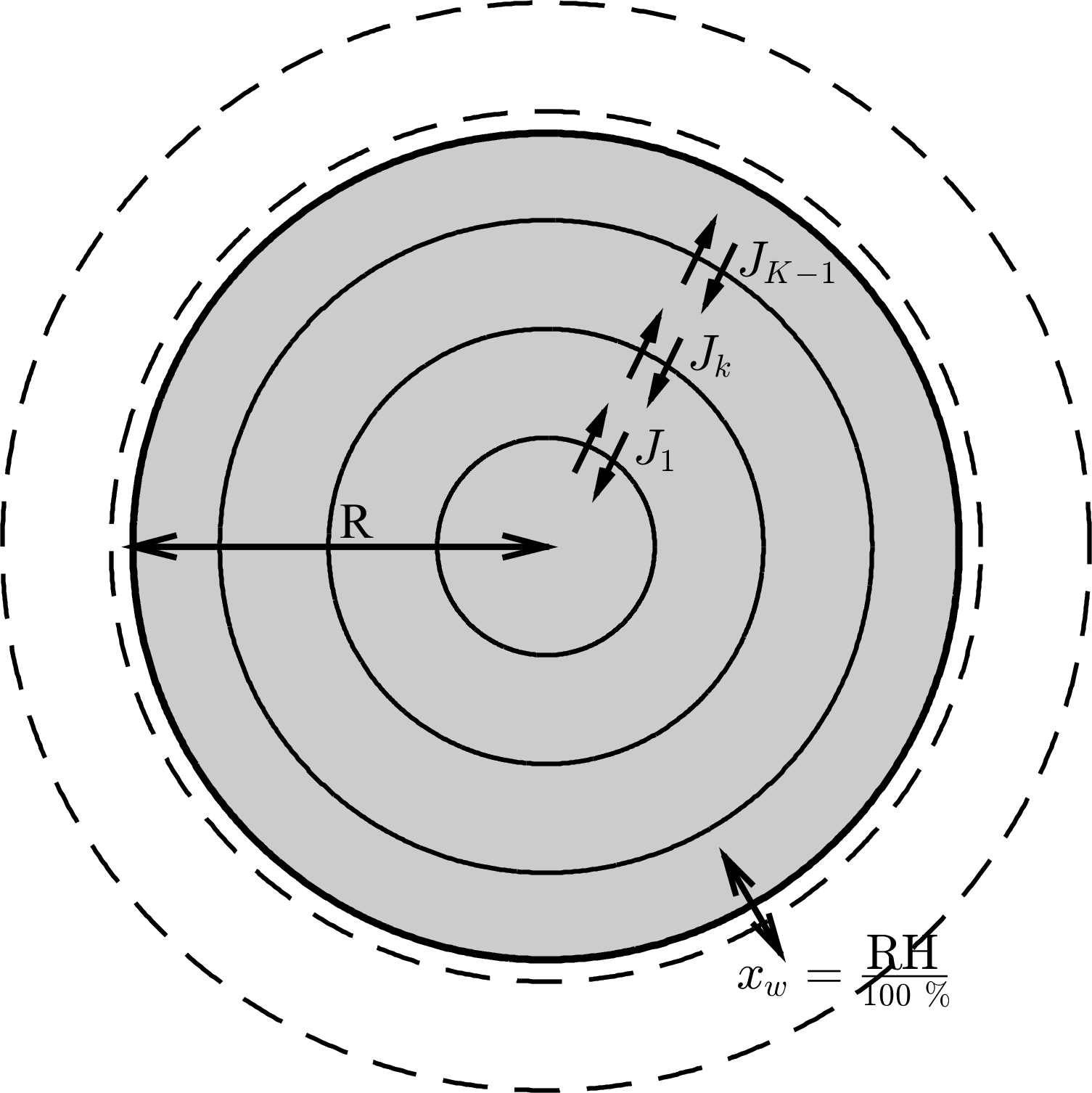
https://www.atmos-chem-phys.net/18/1629/2018/acp-18-1629-2018-f01

Figure 1The aerosol shell model, where diffusion equations are solved numerically to find concentration flux across the shell boundaries. The flux across the outer shell is set to zero, denoted as J_K. However, during each time step water is added to the outer shell to equilibrate it with the surrounding relative humidity, such that $x_{w} = \frac{RH}{100 %}$ . For the purposes of this study it is assumed that the aerosol outer shell equilibrates instantaneously with the ambient conditions in order to investigate the effect of condensed phase diffusion on equilibration timescales. Concentric shells are initialized to be equally spaced – as the aerosol particle grows or shrinks the number of shells in the model increases or decreases. The radius of the outer aerosol shell is variable and acts as a moving boundary to denote the precise size of the particle.

Download

2.1 Fickian framework

By assuming that concentration depends only on time and the radial component, Eq. (2) was solved in a spherically symmetric coordinate system using the backward Euler method of finite differences. After rearranging, the change in concentration between the time steps is related by a tri-diagonal matrix of the form

\begin{matrix} (4) & c_{k}^{n} = α_{k} c_{k - 1}^{n + 1} + β_{k} c_{k}^{n + 1} + γ_{k} c_{k + 1}^{n + 1}, \end{matrix}

where

\begin{array}{l} α_{k} & = - \frac{Δ t r_{n - 1}^{2} D_{k - 1}}{r_{n}^{2} Δ r_{n - \frac{1}{2}} Δ r_{n}}, \\ β_{k} & = 1 - \frac{Δ t r_{n - 1}^{2} D_{k - 1}}{r_{n}^{2} Δ r_{n - \frac{1}{2}} Δ r_{n}} + \frac{Δ t r_{n + 1}^{2} D_{k + 1}}{r_{n}^{2} Δ r_{n + \frac{1}{2}} Δ r_{n}}, \\ γ_{k} & = - \frac{Δ t r_{n + 1}^{2} D_{k + 1}}{r_{n}^{2} Δ r_{n + \frac{1}{2}} Δ r_{n}} . \end{array}

The subscript k corresponds to the shell number and superscript n to the time step. Details of the steps taken during the matrix manipulation are given in the Appendix. In the diffusion step, it was assumed that the organics were involatile; hence there is no external source of material diffusing through the drop, by specifying Neumann flux boundary conditions

\begin{array}{l} \frac{c_{K + 1}^{n + 1} - c_{K - 1}^{n + 1}}{Δ r_{K}} = 0, \\ (5) & \frac{c_{2}^{n + 1} - c_{0}^{n + 1}}{Δ r_{1}} = 0, \end{array}

where the flux through the boundary of the Kth shell is set to zero. Growth of the particle occurs when water is added to the surface shell. Details of the moving boundary are given in the Appendix.

2.2 Maxwell–Stefan framework

The Maxwell–Stefan law of diffusion from Eq. (3) was solved on the aerosol shell model defined in Fig. 1. During the diffusion step we assume that flux at the shell boundary is zero, and consequently find a matrix to solve for the flux across each of the shells given by

\begin{matrix} (6) & [\begin{array}{c} x_{1} \nabla \ln a_{1} \\ x_{2} \nabla \ln a_{2} \\ ⋮ \\ x_{N - 1} \nabla \ln a_{N - 1} \end{array}] = \frac{A}{c^{2}} [\begin{array}{c} J_{1} \\ J_{2} \\ ⋮ \\ J_{N - 1}, \end{array}] \end{matrix}

where A is a matrix defined as

\begin{matrix} (7) & A_{i j} = \{\begin{cases} - \sum_{j \neq i}^{N} (\frac{c_{j}}{Đ_{i j}} + \frac{c_{i} ρ_{N} M_{i}}{Đ_{i N} ρ_{i} M_{N}}) & if i = j, \\ - (\frac{c_{i}}{Đ_{i j}} - \frac{c_{i} ρ_{N} M_{j}}{Đ_{i N} ρ_{j} M_{N}}) & if i \neq j . \end{cases} \end{matrix}

Details of this calculation are given in the Appendix. The solution matrix in Eq. (5) is rearranged to find the diffusion fluxes, J, which are used to find corresponding Fickian diffusion coefficients on the shell boundaries by substituting into Eq. (1). The diffusion coefficients are then used in the numerical solution to Fick's second law in Eq. (4).

In our experiments the organic component is assumed to be non-volatile and only water enters and leaves the aerosol particle. Water is added and removed from the particle at the end of each time step, which allows us to assume that the flux at the shell boundary is zero during the diffusion step. The UNIFAC model is a semi-empirical system that uses both the interactions between functional groups found in the molecules and binary interaction coefficients to calculate the activity coefficients of each component within a solution (Fredenslund et al., 1975). This study uses the UNIFAC group contribution model to estimate the activity coefficients, a_i, in Eq. (3).

2.3 Diffusion coefficients

The Fickian and Maxwell–Stefan diffusion coefficients are both functions of concentration, temperature, pressure and composition. For higher-order systems, the diffusion coefficient describing each component in a mixed solvent is required. This is mathematically expressed as a matrix of individual binary diffusion coefficients.

A mixing rule is used to estimate the relationship of a mutual diffusion coefficient with mole fraction. These mixing rules are based on self-diffusion coefficients of pure substances, found at the limits of mole fraction, D_i,self. Diffusion coefficients in the literature cover a wide range of values (Shiraiwa et al., 2013; Price et al., 2015; Lienhard et al., 2015); hence the self-diffusion coefficients in this study have been chosen to fall within this range in order to investigate model sensitivities.

A variety of different mixing rules have been investigated (O'Meara et al., 2016), however, for the purposes of this study, we have selected the Darken and Vignes relations.

The Darken equation assumes a linear relationship between mole fraction and diffusion coefficient (Darken, 1948),
$\begin{matrix} (8) & Đ_{i j} = x_{i} D_{i, self} + x_{j} D_{j, self} . \end{matrix}$
The Darken relation has been observed to better describe the mixing of ideal liquids (Wesselingh and Bollen, 1997).
The Vignes equation assumes a logarithmic relationship between mole fraction and diffusion coefficient (Vignes, 1966),
$\begin{matrix} (9) & Đ_{i j} = {(D_{i, self})}^{x_{i}} {(D_{j, self})}^{x_{j}} . \end{matrix}$
The Vignes relation is preferred to describe the mixing of viscous fluids, where there is a large difference between their respective self-diffusion coefficients (Wesselingh and Bollen, 1997).

The relationship between water mole fraction and the mutual diffusion coefficient found from the Darken and Vignes mixing rules are shown in Fig. 2.

The Maxwell–Stefan framework separates the ideal and non-ideal effects of diffusion, unlike the Fickian model. Therefore, solutions to the Fickian and Maxwell–Stefan equations only coincide when the mixture is ideal and solubility does not affect the rate of mixing. The two frameworks are related through the so-called thermodynamic factor Γ:

\begin{matrix} (10) & D = Đ Γ . \end{matrix}

The thermodynamic factor gives an effective Fickian diffusion coefficient for the Maxwell–Stefan case (Krishna and Wesselingh, 1997) and is a function of mole fraction and activity coefficient,

\begin{matrix} (11) & Γ_{i j} = δ_{i j} + x_{i} {\frac{\partial \ln a_{i}}{\partial x_{j}}|}_{T, p, x_{k}, k \neq j = 1, 2, \dots, n - 1} \end{matrix}

evaluated at given conditions for temperature T, pressure p and mole fraction x_i, while keeping the mole fraction of all other species, x_k, constant (Taylor and Krishna, 1993), where δ_ij is the Kronecker delta. The resulting diffusion coefficient does provide a non-ideal correction to the Fickian diffusion coefficients. However, it predicts negative diffusion coefficients when the thermodynamic factor becomes negative, which the Fickian framework has not been designed to deal with. The resulting diffusion coefficients are sensitive to the model used to calculate the activity coefficients (Taylor and Krishna, 1993), which is why we have not used the thermodynamic factor as a correction to Fick's laws. Instead, we show the relationship between the thermodynamic factor from Eq. (9) and water mole fraction in Fig. 2 to give an indication of how solubility effects differ between sucrose, butanoic and hexanoic acid.

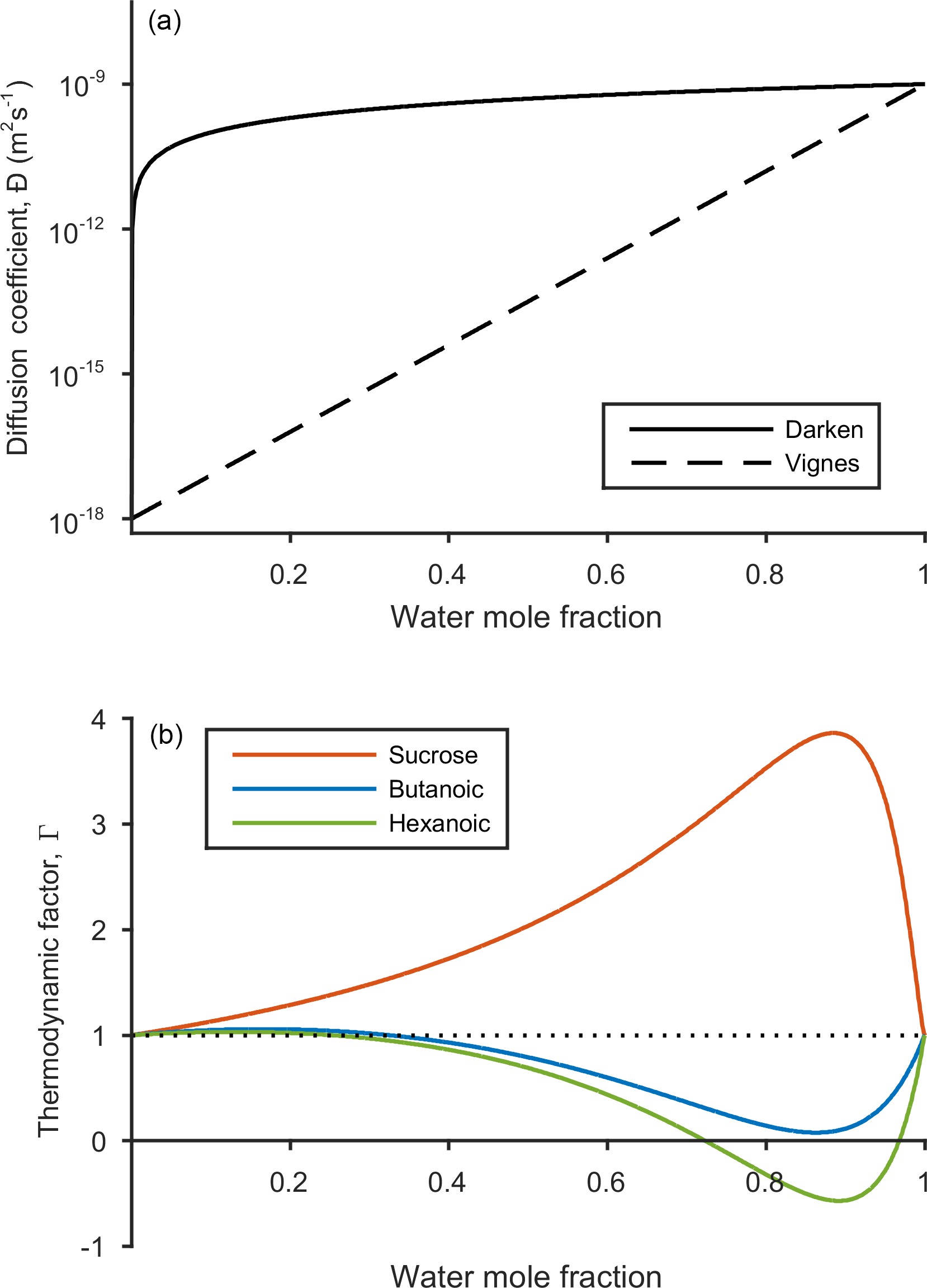
https://www.atmos-chem-phys.net/18/1629/2018/acp-18-1629-2018-f02

Figure 2The dependence of diffusion coefficient and thermodynamic factor on water mole fraction. The solid and dashed black lines represent the Darken and Vignes mixing rules from Eqs. (7) and (8) respectively. The self-diffusion coefficients for water and the non-volatile species are $D_{self} = 1 \times 10^{- 9}$ and $D_{self} = 1 \times 10^{- 18}$ m² s⁻¹ respectively. The thermodynamic factors for sucrose (red), butanoic acid (blue) and hexanoic acid (green) are shown in the lower panel. Phase transitions are indicated when the thermodynamic factor crosses the x axis and equals zero. Activity coefficients used to calculate the thermodynamic factor were found using the UNIFAC model at a temperature of 293.15 K.

Download

3 Results

3.1 General model behaviour

In this study small self-diffusion coefficients of the non-volatile organic compound have been used as a proxy for systems with a pronounced glassy state. To investigate the model sensitivities to viscosity and solubility, the self-diffusion coefficient of the non-volatile compound was varied between 10⁻²⁶ and 10⁻⁹ m² s⁻¹ in the Darken and Vignes mixing rules and the compounds of sucrose, butanoic and hexanoic acid were chosen to simulate a variety non-ideal effects on mixing timescales. The effect of relative humidity on diffusion was also investigated by increasing the equilibrium relative humidity at t=0 from 10 up to 30, 80 and 99 % respectively.

Figures 3 and 4 show the general features of the diffusion frameworks through plots of changes in radial composition with time, after an instantaneous increase in equilibrium relative humidity at t=0. In Figs. 3 and 4, the self-diffusion coefficient of the organic component has been kept constant at $1 \times 10^{- 18}$ m² s⁻¹, so as to focus on the effect of solubility on mixing timescales and particle growth. The ideal Fickian solution acts as a control, where change in aerosol composition with time is modelled without solubility effects arising from intermolecular interactions. Sucrose, butanoic and hexanoic acid provide examples with a spectrum of solubility in water to test the sensitivity of diffusion rates to non-ideal effects.

By first considering the Fickian simulations in Figs. 3 and 4 we are able to focus on the general model behaviour that relates to the ideal effects of diffusion, which in our simulations relate to the Darken and Vignes mixing rules respectively. There are two key differences between the simulations. The first is the timescale of diffusion, and the second is the gradient of the diffusion front. These features have also been noted in previous modelling studies (O'Meara et al., 2016). At low water mole fractions, where the relative humidity is increased from 10 to 30 % the Vignes simulations equilibrate on the scale of seconds, which is 6 orders of magnitude greater than the Darken mixing rule in Fig. 3 predicts. However, at high water mole fractions, when the relative humidity is increased from 10 to 99 %, the timescales of diffusion are more alike. This difference in diffusion timescales between the two mixing rules can be related to the diffusion coefficients in Fig. 2. At low water mole fractions the difference between the Darken and Vignes mixing rules is large, whereas at high water mole fractions the difference between the two mixing rules is smaller.

Now we move on to discuss the Maxwell–Stefan simulations of sucrose, butanoic and hexanoic acids, which also take into account the non-ideal effects of diffusion through the activity coefficients from the UNIFAC model, which is assuming the liquid state. First notice that there is little difference between any of the simulations when relative humidity was instantaneously increased from 10 to 30 % in the first column of both Figs. 3 and 4. The effects of solubility have a negligible impact on the rate of diffusion at low water mole fractions, as Fig. 2 shows that thermodynamic factors do not diverge significantly at water mole fractions less than 0.3.

In the cases where relative humidity has been instantaneously increased from 10 to 80 %, the variation in growth rates and aerosol composition is greater than when relative humidity is increased to 30 %. Variation in mixing timescales can be explained by the diverging thermodynamic factors at high water mole fractions in Fig. 2. It is the polarity of molecules in solution that determines their ability to mix, and water molecules are particularly polar due to the position of hydrogen atoms and the permanent dipole moment. Polar molecules, such as sucrose, are more likely to mix with water as intermolecular bonds form between solute and solvent, which releases energy and further disrupts intermolecular forces between the solute particles and leads to mixing. In contrast, non-polar molecules or sections of molecules, such as alkyl chains, tend to aggregate within water due to hydrophobicity. Monocarboxylic acids are an example of this, as a COOH functional group is positioned at the end of an alkyl chain. As the length of the alkyl chain increases from butanoic to hexanoic, we show that in both the Darken and Vignes examples the rate of mixing reduces significantly due to the greater hydrophobic tendency.

As expected, in Figs. 3 and 4 we find that sucrose grows more quickly than the ideal Fickian case when relative humidity is increased from 10 to 80 or 99 %, reaching equilibrium in almost half the time of the ideal case. The difference in equilibration times shows that solubility needs to be taken into consideration when modelling the change in composition of atmospheric aerosol particles with time, particularly at high water mole fractions.

Butanoic and hexanoic acid, which are the immiscible examples in Figs. 3 and 4, are more interesting. The shorter chain monocarboxylic acid, butanoic acid, containing four carbon atoms, diffuses at a slower rate than the Fickian case, as water on the surface of the particle is inhibited from diffusing into the centre of the particle. The slower rate of mixing corresponds to a thermodynamic factor which is between zero and one at high water mole fractions for butanoic acid, as shown in Fig. 2. Figures 3 and 4 show that under an instantaneous increase in relative humidity from 10 to 80 and 99 % an aerosol particle of hexanoic acid does not grow and equilibrate with the ambient conditions. At high water mole fractions, Fig. 2 shows that the thermodynamic factor for hexanoic acid is negative, corresponding to backwards diffusion against the concentration gradient, which is not expected in the Fickian sense of diffusion. We also find that butanoic acid equilibrates on a significantly slower timescale when the Vignes mixing rule is used with the Maxwell–Stefan framework, which shows that there is a complex interplay between the viscous and soluble effects of diffusion that needs to be better understood.

The simulations in Figs. 3 and 4 were chosen to demonstrate the efficacy of the numerical framework through their wide range of aqueous solubility. For such systems that potentially exhibit a range of amorphous states, it has been hypothesized that combination of absorption and adsorption is needed to explain observed hygroscopicity curves (Pajunoja et al., 2015). In each simulation here, diffusion is controlled by an equilibrated surface mole fraction and predictions from the UNIFAC model. For our model setup, there is a marginally larger water content in the hexanoic acid core after the 10–80 % increase over the 10–99 % increase. For the Darken case in Fig. 3, when relative humidity is increased to 80 % the hexanoic particle equilibrates at a water mole fraction of 0.57. However, when relative humidity is instantaneously increased to 99 %, the hexanoic core equilibrates to a water mole fraction of 0.54 and a shell of water mole fraction greater than 0.95 develops. We believe that the formation of a shell arises as the thermodynamic factor of hexanoic acid in Fig. 2 equals zero at two points, at approximate water mole fractions of 0.7 and 0.95. When the thermodynamic factor vanishes at these two points no further diffusion takes place – hence a clear discontinuity between the two different concentrations of the solution. This cannot be referred to as a liquid–liquid phase separation as schlieren are not included in our simple model to initiate a second phase (Ciobanu et al., 2009). However, our findings still support laboratory evidence of liquid–liquid phase separations forming under conditions of high relative humidities (Renbaum-Wolff et al., 2016). In these studies the volatile liquid component is enclosed in the core of the aerosol particle, which suggests there are other surface effects that are not included into these simple diffusion models. The slight difference in water mole fraction of the equilibrated hexanoic acid core is a result of our numerical approach to solving the diffusion equations for the aerosol framework. In order to find the flux across shell boundaries we use the average concentration of the shells on either side. This may also be the reason that the hexanoic cores equilibrate at lower water mole fractions than the predicted 0.7 based on the thermodynamic factor in Fig. 2. In future work, we propose to combine the core numerical approach presented here with other processes likely taking place that need to be considered with the history of the particle and radial composition heterogeneity.

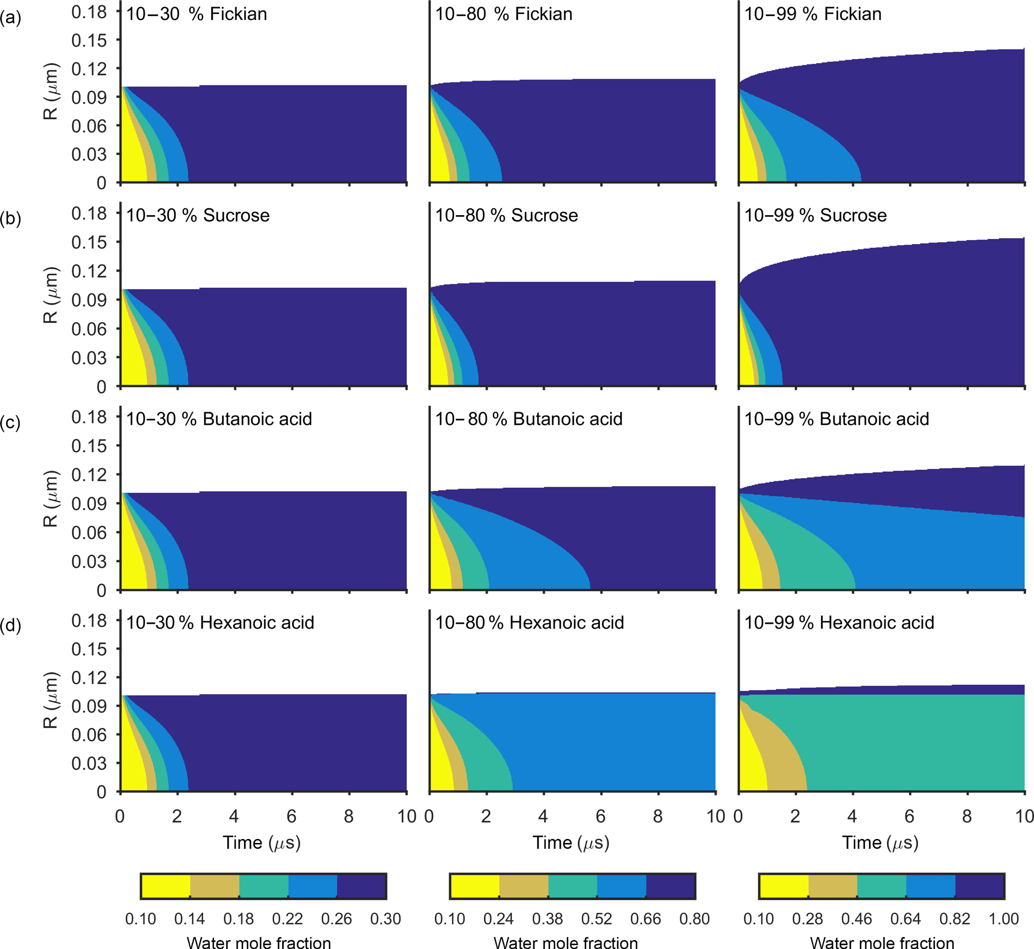
https://www.atmos-chem-phys.net/18/1629/2018/acp-18-1629-2018-f03

Figure 3The change in water mole fraction as a function of radius through time after an initial increase in relative humidity from 10 to 30, 80 and 99 %, at t=0 in the left and right column respectively. Note that there is a different colour scale for each column to ensure clarity in the rate of mixing. The rows correspond to different non-volatile substances, with an arbitrary ideal species in the Fickian case, sucrose, butanoic acid and hexanoic acid from top to bottom. These simulations correspond to the Darken diffusion coefficient and thermodynamic factors given in Fig. 2. The aerosol particles were initialized with a radius of $1 \times 10^{- 7}$ m and the self-diffusion coefficient of water and non-volatile as $D_{self} = 1 \times 10^{- 9}$ and $D_{self} = 1 \times 10^{- 18}$ m² s⁻¹ respectively. The simulations were run at a temperature of 293.15 K.

Download

https://www.atmos-chem-phys.net/18/1629/2018/acp-18-1629-2018-f04

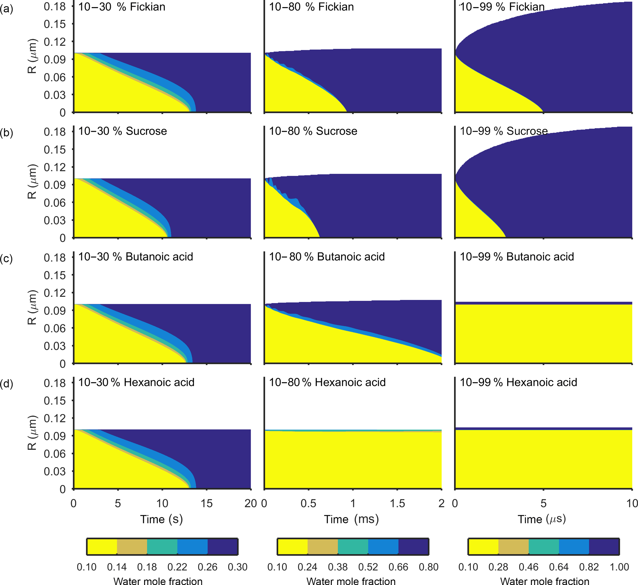
Figure 4The change in water mole fraction as a function of radius through time after an initial increase in relative humidity from 10 to 30, 80 and 99 %, at t=0 in the left and right column respectively. Note that there is a different colour scale for each column to ensure clarity in the rate of mixing. The rows correspond to different non-volatile substances, with an arbitrary ideal species in the Fickian case, sucrose, butanoic acid and hexanoic acid from top to bottom. These simulations correspond to the Vignes diffusion coefficient and thermodynamic factors given in Fig. 2. The aerosol particles were initialized with a radius of $1 \times 10^{- 7}$ m and the self-diffusion coefficient of water and non-volatile as $D_{self} = 1 \times 10^{- 9}$ and $D_{self} = 1 \times 10^{- 18}$ m² s⁻¹ respectively. The simulations were run at a temperature of 293.15 K.

Download

3.2 Model sensitivities

e-folding time has been used previously by Zaveri et al. (2014) and O'Meara et al. (2016) to compare equilibration timescales. The e-folding time is defined as the time it takes for the difference in surface and bulk concentration to change by an exponential factor. Details of this metric and how it is calculated can be found in the Appendix. Figure 5 shows the results of the sensitivity of e-folding time to viscosity and solubility. Solubility has been varied through activity coefficients in Eq. (3) and the viscosity of the solution through self-diffusion coefficients in Eqs. (7) and (8). For this study the self-diffusion coefficient of water has been kept constant at $2 \times 10^{- 9}$ m² s⁻¹ and the self-diffusion coefficient of the second compound has been varied along the x axis. The y axis shows the effect of initial particle radius on e-folding time. Figures 3 and 4 showed that hexanoic acid did not equilibrate when relative humidity is increased instantaneously from 10 to 80 % and therefore does not reach the e-folding time criteria. Hence sucrose and butanoic acid have been used to show how a spectrum of solubility can effect equilibration times through the red and blue lines respectively, in Fig. 5. Throughout the experiment the equilibration timescales were compared back to the Fickian solution, shown by the black dashed line in Fig. 5, which does not take into account the non-ideal effects of diffusion.

Figure 5 shows e-folding time contours as a function of aerosol self-diffusion coefficient and initial radius. We found that changing the mixing rule between Darken and Vignes affected the gradient of the e-folding line contour. In the Darken case, e-folding contours are horizontal, indicating that equilibration times are independent of the self-diffusion coefficient of the non-volatile organic compound and the size of the particle has the biggest influence on equilibration time. By referring back to Fig. 2, we see that the Darken mutual diffusion coefficient on a logarithmic scale of diffusion coefficients is around $1 \times 10^{- 9}$ m² s⁻¹, which is the self-diffusion coefficient of water, the volatile component. In comparison, the Vignes mixing rule gives e-folding time contours with a positive gradient in Fig. 5, as a result of the more significant role of the self-diffusion coefficient of the non-volatile component in Eq. (8).

Through investigating both high and low water mole fractions by increasing the relative humidity from 10 to 30 and 80 % in Fig. 5, we show how the spectrum of solubility translates to equilibration timescales. In both the Vignes and Darken cases solubility does not show a spread of equilibration times when water mole fractions are low and relative humidity is increased from 10 to 30 %. However, when relative humidity is increased from 10 to 80 % solubility becomes a more important factor as the grey area shows the spread in the conditions for the e-folding time contours.

Figure 5 also highlights the plasticizing effect of water within the aerosol system, as at low water mole fractions equilibration times are significantly longer than at high water mole fractions, especially in the Vignes case. Here we have shown that there is a complex interaction between viscosity, solubility and humidity of equilibration timescales, which is important to understand due to the abundance on water in the atmosphere.

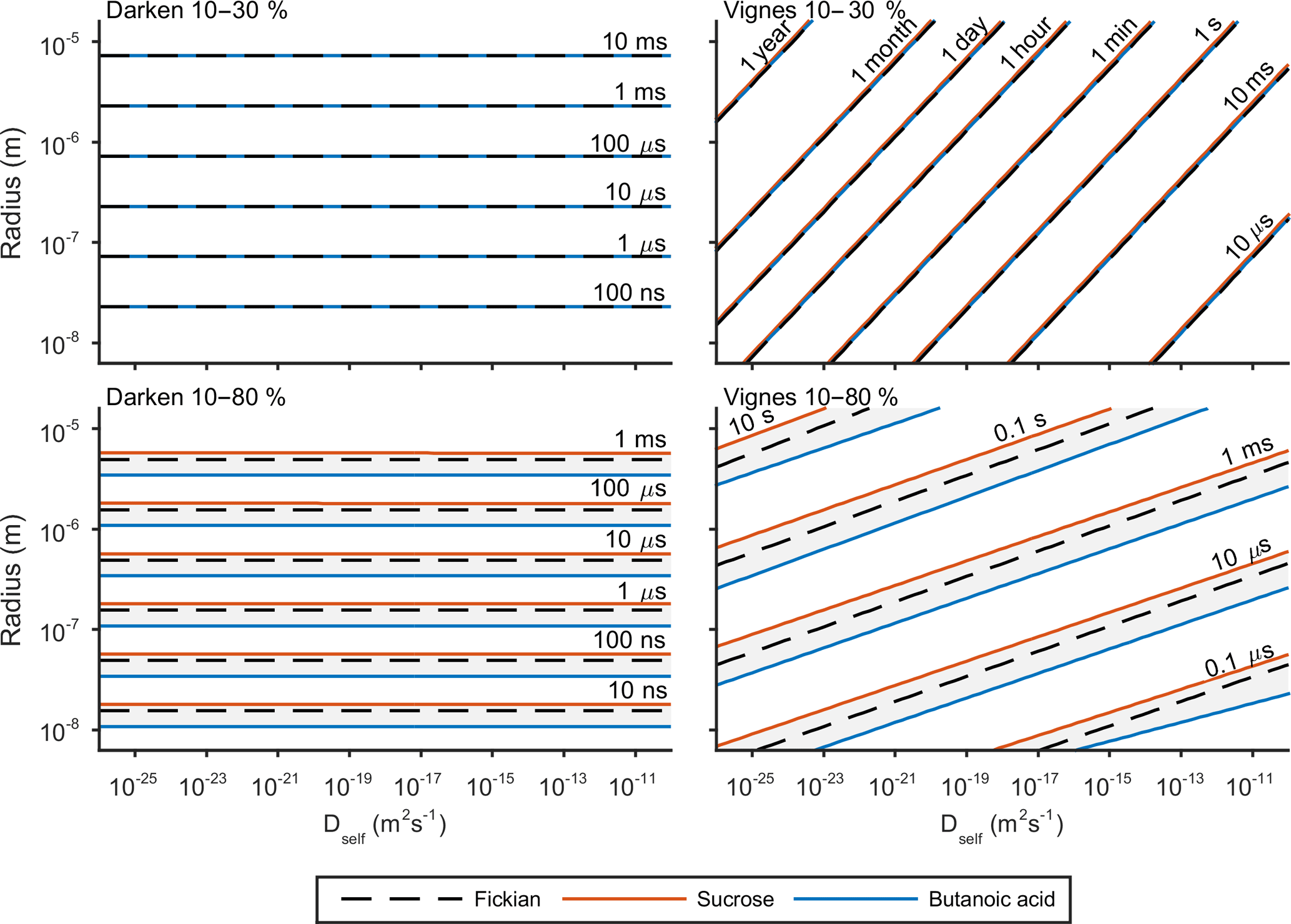
https://www.atmos-chem-phys.net/18/1629/2018/acp-18-1629-2018-f05

Figure 5The e-fold time contours for both the Darken and Vignes mixing rules and how they depend on initial particle radius and self-diffusion coefficient of the non-volatile organic compound. In both cases e-folding times have been found for increases in relative humidity from 10 to 30 and 80 %. The black dashed line represents the e-fold contour found using the Fickian framework. The grey shaded area represents the sensitivity in the model due to the range in solubility between sucrose and butanoic acid given by the red and blue lines respectively. The simulations were run at a temperature of 293.15 K with initially 30 shells equally distributed across the radius of the particle.

Download

4 Conclusions

The main aim of this study has been to introduce the Maxwell–Stefan law of diffusion to describe the changing composition of atmospheric aerosol particles with time. The Maxwell–Stefan equation could act as an alternative framework to the widely used Fickian framework, which has limitations as it does not inherently account for solubility effects. From comparing the sensitivities of these models we found the following:

Observed aerosol partitioning in laboratory studies cannot be replicated using a Fickian framework, which is driven by a gradient in concentration without modifying the Fickian diffusion coefficient to account for the non-ideal effects.
Inclusion of the solubility effects arising from intermolecular interactions is essential to model sustained component separations within aerosol particles. The Maxwell–Stefan framework accounts for these through activity coefficients, calculated using the UNIFAC model.
At low water mole fractions, viscosity was shown to be the most influential factor on equilibration times within aerosol particles.
At high water mole fractions, the variation in equilibration timescales is due to solubility effects, which is especially significant in the atmosphere where there is an abundance of water.
Through simple binary systems of water and a non-volatile secondary organic aerosol, we have shown that there is a complicated relationship between the viscous and soluble effects of mixing. Atmospheric particles are far more complicated systems, with a far greater number of components, all with differing properties. Therefore it is essential to ensure the most suitable framework is used to model this system.

This area of research aims to understand the key micro-physical processes that underpin cloud development and therefore produce models that better predict these processes. We found that at low water mole fractions, equilibration times were most sensitive to changes in viscosity. However at high water mole fractions solubility became a more important factor to consider. This could have significant implications for atmospheric processes – especially for the activation of cloud condensation nuclei and ice nuclei, which occur at high water mole fractions.

This study highlights one key question that needs to be addressed before we continue to investigate the impact of partitioning within aerosol particles on atmospheric models, which is whether current frameworks used to model aerosol composition are suitable to apply to highly complex atmospheric systems. The Fickian model works well for simple two-component systems, where diffusion coefficients can be measured directly. However, for complex systems with multiple components, the Maxwell–Stefan framework offers an alternative which allows mixing against the concentration gradient and phase separations to form.

The Fickian approach has been preferred, as direct measurements of mixing based on equilibration timescales gives a mutual Fickian diffusion coefficient. However, the application of these binary diffusion coefficients to complex, multicomponent atmospheric systems is questionable. On the other hand, the Maxwell–Stefan laws are inherently multicomponent. The difficulty we have is selecting the most appropriate mixing rule, which relates a mutual diffusion coefficient to mole fraction as a function of the self-diffusion coefficients at infinite dilution. Predictive models for Maxwell–Stefan diffusivities have been found experimentally from self-diffusion coefficients (Xin, 2013) and can also be accessed theoretically using molecular dynamic simulations in the region of infinite dilution, where thermodynamic factors can be neglected (Xin, 2013; Krishna and van Baten, 2010 a, b). In this study the Darken and Vignes mixing rules have been investigated, but alternatives such as a constant relationship or a sigmoidal relationship should also be considered (O'Meara et al., 2016). Further investigation is needed to decide which of the relationships are most appropriate and also whether they capture the complexity of multicomponent systems under a range of conditions.

To ultimately answer the question of whether current frameworks describing aerosol composition successfully model atmospheric processes, more laboratory studies are required to test model predictions. Through these investigations, we will then be able to better understand the competition between viscosity (or phase state) and solubility to dominate partitioning within atmospheric aerosol particles.

Code availability

The code has been made open access at https://doi.org/10.5281/zenodo.1156927 (Fowler et al., 2018).

Appendix A: Numerical method

A1 Solving Fick's second law of diffusion using the backward Euler method

Fick's second law predicts how concentration changes with time,

\begin{matrix} (A1) & \frac{\partial c}{\partial t} = \nabla \cdot D \nabla c, \end{matrix}

where c(r,t) is the solute concentration. For an aerosol particle we assume that the concentration only depends upon the radius in a spherically symmetric coordinate system,

\begin{matrix} (A2) & \frac{\partial c}{\partial t} = \frac{1}{r^{2}} \frac{\partial}{\partial r} (D r^{2} \frac{\partial c}{\partial r}) . \end{matrix}

In order to solve this numerically the backward Euler method of finite differences was applied to give

\begin{array}{l} \frac{c_{k}^{n + 1} - c_{k}^{n}}{Δ t} & = \frac{1}{r_{k}^{2} Δ r_{k}} [D_{k + 1} r_{k + 1}^{2} (\frac{c_{k + 1}^{n + 1} - c_{k}^{n + 1}}{Δ r_{k + \frac{1}{2}}}) \\ (A3) & - D_{k - 1} r_{k - 1}^{2} (\frac{c_{k}^{n + 1} - c_{k - 1}^{n + 1}}{Δ r_{k - \frac{1}{2}}})] . \end{array}

Rearranging this equation so all future time steps appear on one side of the equation gives a tri-diagonal matrix of the form

\begin{matrix} (A4) & c_{k}^{n} = α_{k} c_{k - 1}^{n + 1} + β_{k} c_{k}^{n + 1} + γ_{k} c_{k + 1}^{n + 1}, \end{matrix}

where

\begin{array}{l} α_{k} & = - \frac{Δ t r_{k - 1}^{2} D_{k - 1}}{r_{k}^{2} Δ r_{k - \frac{1}{2}} Δ r_{k}}, \\ β_{k} & = 1 - \frac{Δ t r_{k - 1}^{2} D_{k - 1}}{r_{k}^{2} Δ r_{k - \frac{1}{2}} Δ r_{k}} + \frac{Δ t r_{k + 1}^{2} D_{k + 1}}{r_{k}^{2} Δ r_{k + \frac{1}{2}} Δ r_{k}}, \\ γ_{i} & = - \frac{Δ t r_{k + 1}^{2} D_{k + 1}}{r_{k}^{2} Δ r_{k + \frac{1}{2}} Δ r_{k}} . \end{array}

To solve this equation it was assumed that there was no external source of material diffusing through the drop. We specify Neumann boundary conditions, where the flux through the shell boundary is set to zero. The flux conditions are given as

\begin{matrix} (A5) & \begin{aligned} \frac{c_{K + 1}^{n + 1} - c_{K - 1}^{n + 1}}{Δ r_{K}} & = 0, \\ \frac{c_{2}^{n + 1} - c_{0}^{n + 1}}{Δ r_{1}} & = 0, \end{aligned} \end{matrix}

which means that elements in the first and last rows of the matrix are adjusted to agree with this condition.

A2 Solving Maxwell–Stefan equation for an aerosol particle

We begin with the Maxwell–Stefan equation

\begin{matrix} (A6) & x_{i} \nabla \ln a_{i} = - \sum_{j = 1, j \neq i}^{N} \frac{c_{i} J_{j} - c_{j} J_{i}}{c^{2} Đ_{i j}} . \end{matrix}

By specifying that the Nth volume flux is equal to the negative sum of all other volume fluxes, therefore not allowing an external source of material to enter the particle, we can define a reference frame in which to solve the problem. Rewriting the equation gives

\begin{matrix} (A7) & x_{i} \nabla \ln a_{i} = \frac{c_{i} J_{N}}{c^{2} Đ_{i N}} - \sum_{j = 1, j \neq i}^{N} \frac{c_{j} J_{i}}{c^{2} Đ_{i j}} + \sum_{j = 1, j \neq i}^{N - 1} \frac{c_{i} J_{j}}{c^{2} Đ_{i j}}, \end{matrix}

where

\begin{matrix} (A8) & \begin{aligned} J_{N} & = - \frac{ρ_{N}}{M_{N}} \sum_{j = 1}^{N - 1} \frac{M_{j} J_{j}}{ρ_{j}}, \\ = - \frac{ρ_{N}}{M_{N}} \frac{M_{i} J_{i}}{ρ_{i}} - \frac{ρ_{N}}{M_{N}} \sum_{j \neq 1}^{N - 1} \frac{M_{j} J_{j}}{ρ_{j}}, \end{aligned} \end{matrix}

where ρ_i and M_i correspond to the density and mass of shell i. Substituting this into Eq. (A6) yields

\begin{array}{l} x_{i} \nabla \ln a_{i} & = \frac{J_{i}}{c^{2}} (\frac{c_{i} ρ_{N} M_{i}}{Đ_{i N} ρ_{i} M_{N}} - \sum_{j = 1, j \neq i}^{N} \frac{c_{j}}{Đ_{i j}}) \\ (A9) & + \sum_{j = 1, j \neq i}^{N - 1} \frac{J_{j}}{c^{2}} (\frac{c_{i}}{Đ_{i j}} - \frac{c_{i} ρ_{N} M_{j}}{Đ_{i N} ρ_{j} M_{N}}) . \end{array}

The numerical model is solved using matrix algebra and written in that form gives

\begin{matrix} (A10) & [\begin{array}{c} x_{1} \nabla \ln a_{1} \\ x_{2} \nabla \ln a_{2} \\ ⋮ \\ x_{N - 1} \nabla \ln a_{N - 1} \end{array}] = \frac{A}{c^{2}} [\begin{array}{c} J_{1} \\ J_{2} \\ ⋮ \\ J_{N - 1} \end{array}], \end{matrix}

where A is a matrix defined as

\begin{matrix} (A11) & A_{i j} = \{\begin{cases} - \sum_{j \neq i}^{N} (\frac{c_{j}}{Đ_{i j}} + \frac{c_{i} ρ_{N} M_{i}}{Đ_{i N} ρ_{i} M_{N}}) & if i = j, \\ - ({\frac{c_{i}}{Đ}}_{i j} - \frac{c_{i} ρ_{N} M_{j}}{Đ_{i N} ρ_{j} M_{N}}) & if i \neq j . \end{cases} \end{matrix}

A3 Moving boundary

Each time step is separated into a diffusion step and a moving boundary step, which allows the amount of water in the particle to change. This was not used during the model runs in this paper. However, the development of a moving boundary is vital for the inclusion of a diffusion step into a parcel model and to investigate the effect of aerosol composition on cloud micro-physical properties.

If the change in volume is positive and water is deposited onto the surface of the aerosol particle, then the steps involved to change the outer boundary of the particle are as follows:

The new radius, R, of the particle is found, based on the change in volume, ΔV.
The change in volume is then used to calculate the molar concentration in the outer shell as follows:
$\begin{matrix} (A12) & x_{w}^{n + 1} = x_{w}^{n} + \frac{Δ V ρ_{w}}{M_{w}}, \end{matrix}$
where n corresponds to the time step.
Shell boundaries are then initiated and filled with the total moles in each layer. If the final shell is filled the molar concentration is distributed over to a new shell; see Fig. 1.
Shell boundaries are initially fixed distances apart, however in the final step, the outer shell radius, R_K is changed to the same as the new radius, R, calculated in the first step, such that R_K=R, as in Fig. 1.

If the change in volume is negative and water is being removed from the particle surface, then the steps involved to change the outer boundary of the particle are as follows:

The total volume of water is calculated as sum of the volume of each individual shell V_k, the molar concentration of each shell c_k, molar mass of water M_w and the density of water ρ_w,
$\begin{matrix} (A13) & V_{w} = \sum_{k = 1}^{K} \frac{c_{k} V_{k} M_{w}}{ρ_{w}} . \end{matrix}$
Only water is removed from the aerosol particle, therefore if V_w=0 then there are no changes to the particle volume, if V_w<ΔV then all of the water is removed from the particle and if V_w>ΔV, water is first removed from the outer shells and replaced by with other components.
After the water has been removed, a new outer shell radius is found,
$\begin{matrix} (A14) & R_{K} = {({R_{K - 1}}^{3} - \frac{3 M_{s} N_{s}}{4 π ρ_{s}})}^{\frac{1}{3}}, \end{matrix}$
where R_K is the new radius of the outer shell and the subscript corresponds the number of the shell, N_s is the number of moles of solute in the Kth shell, M_s and ρ_s are the molar mass and density of the compound respectively; see Fig. 1.

Appendix B: Model testing

B1 Model initialization

This study has assumed that the mole fraction of water in the condensed phase in the outer shell is in equilibration with the ambient saturation relative humidity. This assumes ideality of the accommodation coefficient, which enables the study to focus on the sensitivity of diffusion timescales to the framework used. The equation for water mole fraction,

\begin{matrix} (B1) & x_{w} = \frac{N_{w}}{N_{w} + N_{s}}, \end{matrix}

where N_w and N_s are the number of molecules of water and the solute in the outer shell respectively, and the equation for the volume of the outer shell,

\begin{matrix} (B2) & V = N_{w} (\frac{M_{w}}{ρ_{w}}) + N_{s} (\frac{M_{s}}{ρ_{s}}), \end{matrix}

was used to find the volume of water to be added or removed from the system in order to keep the outer shell equilibrated with the saturation relative humidity. In this study the molar mass and density of the solute were kept constant at M_s=400 g mol⁻¹ and $ρ_{s} = 1.5 \times 10^{3}$ kg m⁻³. For water these values were M_w=18 g mol⁻¹ and $ρ_{s} = 1 \times 10^{3}$ kg m⁻³.

B2 e-folding time

To find the e-folding time of a system, first the ratio Q is defined as

\begin{matrix} (B3) & Q = \frac{{|C_{s} - {\overline{C}}_{b}|}_{t \geq 0}}{{|C_{s} - {\overline{C}}_{b}|}_{t = 0}}, \end{matrix}

where C_s is the surface shell concentration and ${\overline{C}}_{b}$ bulk concentration (O'Meara et al., 2016). The e-folding time is then defined as the time when the difference between surface shell and bulk concentration changes by an exponential factor. Numerically this is $Q = e^{- 1} .$

Competing interests

The authors declare that they have no conflict of interest.

Acknowledgements

This work was funded by the Natural Environment Research Council (NERC) through the PhD studentship of Kathryn Fowler under the grant reference number NE/L002469/1. Paul J. Connolly acknowledges funding from the European Union's Seventh Framework Programme (FP7/2007-2013) under grant agreement number 603445 EU FP7.

Edited by: Yafang Cheng
Reviewed by: two anonymous referees

References

Boucher, O., Randall, D., Artaxo, P., Bretherton, C., Feingold, G., Forster, P., Kerminen, V.-M., Kondo, Y., Liao, H., Lohmann, U., Rasch, P., Satheesh, S. K., Sherwood, S., Stevens, B., and Zhang, X. Y.: Clouds and Aerosols, in: Climate Change 2013: The Physical Science Basis, Contribution of Working Group I to the Fifth Assessment Report of the Intergovernmental Panel on Climate Change, edited by: Stocker, T. F., Qin, D., Plattner, G.-K., Tignor, M., Allen, S. K., Boschung, J., Nauels, A., Xia, Y., Bex, V., and Midgley, P. M., Cambridge University Press, Cambridge, United Kingdom and New York, NY, USA, 571–658, https://doi.org/10.1017/CBO9781107415324.016, 2013. a

Ciobanu, V. G., Marcolli, C., Krieger, U. K., Weers, U., and Peter, T.: Liquid-Liquid Phase Separation in Mixed Organic/Inorganic Aerosol Particles, J. Phys. Chem. A, 113, 10966–10978, https://doi.org/10.1021/jp905054d, 2009. a

Darken, L. S.: Diffusion, mobility and their interrelation through free energy in binary metallic systems, Trans. Aime, 175, 184–201, https://doi.org/10.1007/s11661-010-0177-7, 1948. a, b

Fick, A.: Ueber Diffusion, Annalen der Physik und Chemie, 170, 59–86, https://doi.org/10.1002/andp.18551700105, 1855. a

Fowler, K., Connolly, P. J., Topping, D. O., and O'Meara, S.: Maxwell-Stefan diffusion: a framework for predicting condensed phase diffusion and phase separation in atmospheric aerosol (Supporting code), Zenodo, https://doi.org/10.5281/zenodo.1161213, 2018.

Fredenslund, A., Jones, R. L., and Prausnitz, J. M.: Group-contribution estimation of activity coefficients in nonideal liquid mixtures, AIChE J., 21, 1086–1099, https://doi.org/10.1002/aic.690210607, 1975. a

Krishna, R. and van Baten, J. M.: Hydrogen bonding effects in adsorption of water-alcohol mixtures in zeolites and the consequences for the characteristics of the Maxwell–Stefan diffusivities, Langmuir, 26, 10854–10867, https://doi.org/10.1021/la100737c, 2010a. a

Krishna, R. and van Baten, J. M.: Highlighting pitfalls in the Maxwell–Stefan modeling of water-alcohol mixture permeation across pervaporation membranes, J. Membrane Sci., 360, 476–482, https://doi.org/10.1016/j.memsci.2010.05.049, 2010b. a

Krishna, R. and Wesselingh, J.: The Maxwell-Stefan approach to mass transfer, Chem. Eng. Sci., 52, 861–911, https://doi.org/10.1016/S0009-2509(96)00458-7, 1997. a, b

Lienhard, D. M., Huisman, A. J., Bones, D. L., Te, Y.-F., Luo, B. P., Krieger, U. K., and Reid, J. P.: Retrieving the translational diffusion coefficient of water from experiments on single levitated aerosol droplets, Phys. Chem. Chem. Phys., 16, 16677–16683, https://doi.org/10.1039/c4cp01939c, 2014. a, b

Lienhard, D. M., Huisman, A. J., Krieger, U. K., Rudich, Y., Marcolli, C., Luo, B. P., Bones, D. L., Reid, J. P., Lambe, A. T., Canagaratna, M. R., Davidovits, P., Onasch, T. B., Worsnop, D. R., Steimer, S. S., Koop, T., and Peter, T.: Viscous organic aerosol particles in the upper troposphere: diffusivity-controlled water uptake and ice nucleation?, Atmos. Chem. Phys., 15, 13599–13613, https://doi.org/10.5194/acp-15-13599-2015, 2015. a, b, c, d

Mikhailov, E., Vlasenko, S., Martin, S. T., Koop, T., and Pöschl, U.: Amorphous and crystalline aerosol particles interacting with water vapor: conceptual framework and experimental evidence for restructuring, phase transitions and kinetic limitations, Atmos. Chem. Phys., 9, 9491–9522, https://doi.org/10.5194/acp-9-9491-2009, 2009. a

O'Meara, S., Topping, D. O., and McFiggans, G.: The rate of equilibration of viscous aerosol particles, Atmos. Chem. Phys., 16, 5299–5313, https://doi.org/10.5194/acp-16-5299-2016, 2016. a, b, c, d, e, f, g, h, i

Pajunoja, A., Lambe, A. T., Hakala, J., Rastak, N., Cummings, M. J., Brogan, J. F., Hao, L., Paramonov, M., Hong, J., Prisle, N. L., Malila, J., Romakkaniemi, S., Lehtinen, K. E. J., Laaksonen, A., Kulmala, M., Massoli, P., Onasch, T. B., Donahue, N. M., Riipinen, I., Davidovits, P., Worsnop, D. R., Petäjä, T., and Virtanen, A.: Adsorptive uptake of water by semisolid secondary organic aerosols, Geophys. Res. Lett., 42, 3063–3068, https://doi.org/10.1002/2015GL063142, 2015. a

Pöschl, U., Rudich, Y., and Ammann, M.: Kinetic model framework for aerosol and cloud surface chemistry and gas-particle interactions – Part 1: General equations, parameters, and terminology, Atmos. Chem. Phys., 7, 5989–6023, https://doi.org/10.5194/acp-7-5989-2007, 2007. a

Power, R. M., Simpson, S. H., Reid, J. P., and Hudson, A. J.: The transition from liquid to solid-like behaviour in ultrahigh viscosity aerosol particles, Chem. Sci., 4, 2597, https://doi.org/10.1039/c3sc50682g, 2013. a

Price, H. C., Murray, B. J., Mattsson, J., O'Sullivan, D., Wilson, T. W., Baustian, K. J., and Benning, L. G.: Quantifying water diffusion in high-viscosity and glassy aqueous solutions using a Raman isotope tracer method, Atmos. Chem. Phys., 14, 3817–3830, https://doi.org/10.5194/acp-14-3817-2014, 2014. a

Price, H. C., Mattsson, J., Zhang, Y., Bertram, A. K., Davies, J. F., Grayson, J. W., Martin, S. T., O'Sullivan, D., Reid, J. P., Rickards, A. M. J., and Murray, B. J.: Water diffusion in atmospherically relevant α-pinene secondary organic material, Chem. Sci., 6, 4876–4883, https://doi.org/10.1039/C5SC00685F, 2015. a, b, c, d

Price, H. C., Mattsson, J., and Murray, B. J.: Sucrose diffusion in aqueous solution, Phys. Chem. Chem. Phys., 18, 19207–19216, https://doi.org/10.1039/C6CP03238A, 2016. a

Renbaum-Wolff, L., Song, M., Marcolli, C., Zhang, Y., Liu, P. F., Grayson, J. W., Geiger, F. M., Martin, S. T., and Bertram, A. K.: Observations and implications of liquid-liquid phase separation at high relative humidities in secondary organic material produced by α-pinene ozonolysis without inorganic salts, Atmos. Chem. Phys., 16, 7969–7979, https://doi.org/10.5194/acp-16-7969-2016, 2016. a

Shiraiwa, M., Zuend, A., Bertram, A. K., and Seinfeld, J. H.: Gas-particle partitioning of atmospheric aerosols: interplay of physical state, non-ideal mixing and morphology, Phys. Chem. Chem. Phys., 15, 11441, https://doi.org/10.1039/c3cp51595h, 2013. a, b, c

Song, M., Marcolli, C., Krieger, U. K., Zuend, A., and Peter, T.: Liquid–liquid phase separation and morphology of internally mixed dicarboxylic acids/ammonium sulfate/water particles, Atmos. Chem. Phys., 12, 2691–2712, https://doi.org/10.5194/acp-12-2691-2012, 2012. a

Song, Y. C., Haddrell, A. E., Bzdek, B. R., Reid, J. P., Bannan, T., Topping, D. O., Percival, C., and Cai, C.: Measurements and Predictions of Binary Component Aerosol Particle Viscosity., J. Phys. Chem. A, https://doi.org/10.1021/acs.jpca.6b07835, 2016. a

Taylor, R. and Krishna, R.: Multicomponent Mass Transfer, John Wiley & Sons, Inc., New York, 1993. a, b, c

Vignes, A.: Diffusion in Binary Solutions. Variation of Diffusion Coefficient with Composition, Ind. Eng. Chem. Fund., 5, 189–199, https://doi.org/10.1021/i160018a007, 1966. a, b

Virtanen, A., Joutsensaari, J., Koop, T., Kannosto, J., Yli-Pirilä, P., Leskinen, J., Mäkelä, J. M., Holopainen, J. K., Pöschl, U., Kulmala, M., Worsnop, D. R., and Laaksonen, A.: An amorphous solid state of biogenic secondary organic aerosol particles., Nature, 467, 824–827, https://doi.org/10.1038/nature09455, 2010. a

Wesselingh, J. and Bollen, A.: Multicomponent Diffusivities from the Free Volume Theory, Chem. Eng. Res. Des., 75, 590–602, https://doi.org/10.1205/026387697524119, 1997. a, b

Xin, L.: Diffusion in Liquids: Equilibrium Molecular Simulations and Predictive Engineering Models, available at: http://homepage.tudelft.nl/v9k6y/thesis-xin-liu.pdf (last access: 1 February 2018), 2013. a, b

Ye, Q., Robinson, E. S., Ding, X., Ye, P., Sullivan, R. C., and Donahue, N. M.: Mixing of secondary organic aerosols versus relative humidity, P. Natl. Acad. Sci. USA, 113, 12649–12654, https://doi.org/10.1073/pnas.1604536113, 2016. a

Yli-Juuti, T., Pajunoja, A., Tikkanen, O.-P., Buchholz, A., Faiola, C., Väisänen, O., Hao, L., Kari, E., Peräkylä, O., Garmash, O., Shiraiwa, M., Ehn, M., Lehtinen, K., and Virtanen, A.: Factors controlling the evaporation of secondary organic aerosol from α-pinene ozonolysis, Geophys. Res. Lett., 44, 2562–2570, https://doi.org/10.1002/2016GL072364, 2017. a

Zaveri, R. A., Easter, R. C., Shilling, J. E., and Seinfeld, J. H.: Modeling kinetic partitioning of secondary organic aerosol and size distribution dynamics: representing effects of volatility, phase state, and particle-phase reaction, Atmos. Chem. Phys., 14, 5153–5181, https://doi.org/10.5194/acp-14-5153-2014, 2014. a

Zobrist, B., Soonsin, V., Luo, B. P., Krieger, U. K., Marcolli, C., Peter, T., and Koop, T.: Ultra-slow water diffusion in aqueous sucrose glasses., Phys. Chem. Chem. Phys., 13, 3514–26, https://doi.org/10.1039/c0cp01273d, 2011. a

Zuend, A., Marcolli, C., Peter, T., and Seinfeld, J. H.: Computation of liquid-liquid equilibria and phase stabilities: implications for RH-dependent gas/particle partitioning of organic-inorganic aerosols, Atmos. Chem. Phys., 10, 7795–7820, https://doi.org/10.5194/acp-10-7795-2010, 2010. a

Articles

Short summary

This is the first time the Maxwell–Stefan framework has been applied to an atmospheric aerosol core–shell model and shows that there is a complex interplay between the viscous and solubility effects on aerosol composition. Understanding aerosol composition is essential to accurately model their interactions within atmospheric systems. We use simple binary systems to demonstrate how viscosity and solubility both play a role in affecting the rate of diffusion through aerosol particles.