the Creative Commons Attribution 4.0 License.
the Creative Commons Attribution 4.0 License.
 | 16 Nov 2018
Southern California megacity CO2, CH4, and CO flux estimates using ground- and space-based remote sensing and a Lagrangian model
Jacob K. Hedelius
Junjie Liu
Tomohiro Oda
Shamil Maksyutov
Coleen M. Roehl
Laura T. Iraci
James R. Podolske
Patrick W. Hillyard
Jianming Liang
Kevin R. Gurney
Debra Wunch
Paul O. Wennberg
We estimate the overall CO2, CH4, and CO flux from the South Coast Air Basin using an inversion that couples Total Carbon Column Observing Network (TCCON) and Orbiting Carbon Observatory-2 (OCO-2) observations, with the Hybrid Single Particle Lagrangian Integrated Trajectory (HYSPLIT) model and the Open-source Data Inventory for Anthropogenic CO2 (ODIAC). Using TCCON data we estimate the direct net CO2 flux from the SoCAB to be 104 ± 26 Tg CO2 yr−1 for the study period of July 2013–August 2016. We obtain a slightly higher estimate of 120 ± 30 Tg CO2 yr−1 using OCO-2 data. These CO2 emission estimates are on the low end of previous work. Our net CH4 (360 ± 90 Gg CH4 yr−1) flux estimate is in agreement with central values from previous top-down studies going back to 2010 (342–440 Gg CH4 yr−1). CO emissions are estimated at 487 ± 122 Gg CO yr−1, much lower than previous top-down estimates (1440 Gg CO yr−1). Given the decreasing emissions of CO, this finding is not unexpected. We perform sensitivity tests to estimate how much errors in the prior, errors in the covariance, different inversion schemes, or a coarser dynamical model influence the emission estimates. Overall, the uncertainty is estimated to be 25 %, with the largest contribution from the dynamical model. Lessons learned here may help in future inversions of satellite data over urban areas.


About 43 % of global anthropogenic carbon dioxide (CO2) emissions come directly from urban areas, and urban final energy use accounts for about 76 % of CO2 emissions (Seto and Dhakal, 2014). Associations of cities that recognize their significant emissions of CO2 to the atmosphere – such as the C40 Cities Climate Leadership Group (C40) – seek to reduce their greenhouse gas (GHG) emissions and develop local resilience to changing climate. There is a need to track long-term anthropogenic GHG emissions from urban areas to aid urban planners and ensure commitments are met.
Bottom-up (BU) inventories (e.g., of CO2) can be derived by accounting for various emission activities such as transportation, electricity generation, industry, and heating. BU inventories have some inherent uncertainty due to imperfect emission models, which are largely based on extrapolation of controlled studies and rely on assumptions of fuel consumption, and due to disagreements in downscaling methods (Duren and Miller, 2012; Sargent et al., 2018). Uncertainties in how emissions are calculated and in the underlying activity data used to construct inventories make them susceptible to systematic biases by nature (Oda et al., 2017). On the national level, 2σ uncertainties range from 4.0 % to 17.5 % for the 10 largest emitters (Oda et al., 2018). Uncertainties on the grid cell level are unique to the disaggregation method, but may be in the range of 4 %–190 % (2σ) (Andres et al., 2016). Top-down (TD) emission estimate methods rely on measurements of gases along with models of atmospheric transport, which have their own inherent uncertainties. Measures of emissions and emission changes are generally more reliable when TD and BU methods are in agreement (Duren and Miller, 2012).
Tracking emissions from a TD perspective requires observations. Various networks, such as the Total Carbon Column Observing Network (TCCON) and the National Oceanic and Atmospheric Administration (NOAA) Earth System Research Laboratory (ESRL) in situ CO2 network can aid in long-term measurements but are too sparse to track emissions from more than a few cities. Some urban areas have ground-based networks (Lauvaux et al., 2016; Mitchell et al., 2018; Sargent et al., 2018; Shusterman et al., 2016; Verhulst et al., 2017). Significant progress has been made in minimizing the cost, deployment time, and data delivery from these networks. However, they still require a significant number of personnel hours and are difficult to scale up to more than a few dozen areas for long-term observations. Urban observation networks can provide finer spatial and temporal details on emission sources, but space-based observations are likely the only way to track emissions TD for more than a few dozen cities.
Within the past 10 years, two satellites have been shown to have high-precision (better than 1 ppm) small-footprint (<100 km2) CO2 observing capabilities, including the Greenhouse Gases Observing Satellite (GOSAT, in orbit 2009) and the Orbiting Carbon Observatory-2 (OCO-2, in orbit 2014). Several other satellites are planned or are already in orbit with this same potential. Combined, OCO-2 and GOSAT can cover about 1 % of the Earth's surface every 3 days, and though this is only a small fraction, it is unprecedented. Other missions such as TanSat (in orbit 2016), GAS onboard FY-3D (in orbit 2017), GOSAT-2 (in orbit 2018), OCO-3 (expected 2019), and GeoCARB (expected 2023) may further bolster coverage. Space-based observations of methane (CH4) have been made from GOSAT and the TROPOspheric Monitoring Instrument (TROPOMI, in orbit 2017) and will be made from the GOSAT-2 and planned GeoCARB missions. Carbon monoxide (CO) is measured using Measurements of Pollution in the Troposphere (MOPITT, in orbit 1999) and TROPOMI and will be from GOSAT-2. There is presently a lack of studies that have assimilated satellite trace-gas abundance data into inversion schemes to determine urban emissions.
We test trajectory-based inversion schemes to see if they can reproduce known emissions (from inventories and previous studies) from the California South Coast Air Basin (SoCAB). Our goal is not to apportion spatially, but rather to come up with a single number for the total flux and an estimate of uncertainty. Fluxes from this urban area (pop. ∼ 16.3 million) have been studied extensively, and it provides a test bed to evaluate methods. We discuss the components used to build our inversion in Sect. 2. Typical urban enhancements are described in Sect. 3. Fluxes of CO2, CO, and CH4 using TCCON data and of CO2 using OCO-2 data are discussed in Sect. 4 along with sources of uncertainty. In Sect. 5 we discuss emission ratios, which can also be used to evaluate our flux results. We conclude by summarizing uncertainty and mentioning expansions and areas of improvement in Sect. 6.
2.1 Observations of column-averaged dry-air mole fractions
We use observations of column-averaged dry-air mole fraction (denoted Xgas) to tie model abundances to fluxes. Column averages are calculated by dividing the retrieved amount of the gas of interest (molecules cm−2) by the retrieved total column of dry air (molecules cm−2). Xgas values are less sensitive to changes in surface pressure and water vapor than total column amounts in units of molecules per square centimeter (Wunch et al., 2015).
Data are obtained from the TCCON and OCO-2. We use TCCON data from the California Institute of Technology (Caltech) site in Pasadena, California (Wennberg et al., 2014), and from the NASA Armstrong Flight Research Center (AFRC) site near Lancaster, California (Iraci et al., 2014). Values of , XCO, and were generated using the operational GGG2014 algorithm (Wunch et al., 2015). The Caltech site (lat 34.136, long −118.127, 240 m a.s.l.) is located in an urban environment within the SoCAB. As the name implies, the SoCAB is a basin surrounded by mountains, except towards the southwest, which boarders the Pacific Ocean. AFRC (lat 34.960, long −117.881, 700 m a.s.l.) is located outside the basin ∼100 km to the north in a much more sparsely populated area. Because of the lower population density, the AFRC is often considered a “background” site. However, depending on airflow patterns, recent emissions from the SoCAB may be observed at the AFRC so we use the term background loosely to indicate where lower concentrations are typically observed. Coincident data from both sites are available from July 2013 to August 2016, after which the AFRC instrument was relocated. In total, there are 5355 paired hourly averaged observations on 783 days.
OCO-2 data are available starting September 2014 when the instrument began its nominal operational mission (OCO-2 Science Team et al., 2017). Here, we use data generated using the NASA Atmospheric CO2 Observations from Space (ACOS) version 8r algorithm (O'Dell et al., 2018). We also do a partial analysis on v7r data for comparison with past studies that used these data with a focus on the SoCAB (Hedelius et al., 2017a; Schwandner et al., 2017). Because OCO-2 is in a sun-synchronous orbit with an equatorial crossing time of around 13:00 local solar time, all observations are in the early afternoon. OCO-2 has 8 longitudinal pixels, with a footprint of ∼3 km2 each. To reduce over-weighting target mode observations, OCO-2 data are gridded to . Before filtering there are 6098 pre-averaged OCO-2 observations on 29 different overpass days when the AFRC TCCON site also collected background observations.
In Appendix A we describe filtering, background subtraction, boundary conditions, and our accounting for averaging kernels. In short, we determine enhancements of various gases (ΔXgas) by finding the difference between observations within the basin (either the Caltech TCCON or OCO-2) compared with the AFRC TCCON site.
2.2 A priori flux estimates
Our flux estimate involves scaling the a priori spatial inventory, or subregions of the prior up or down to reduce the measurement–model mismatch. More important than the total prior absolute flux is the distribution of sources. EDGAR (Emissions Database for Global Atmospheric Research; EC-JRC/PBL, 2009) and FFDAS v2.0 (Fossil Fuel Data Assimilation System; Asefi-Najafabady et al., 2014) are available globally at a 0.1∘ resolution. We use the year 2016 version of the Open-source Data Inventory for Anthropogenic CO2 (ODIAC2016), which is available globally at a resolution of 30 arcsec from 2000 to 2015 (Oda and Maksyutov, 2011, 2015; Oda et al., 2018). We also compare total SoCAB emissions from the 2015 version of ODIAC (ODIAC2015), which is based on a projection of the Carbon Dioxide Information Analysis Center (CDIAC) country total emissions. ODIAC has a monthly variation and compared to the annual average seasonal flux ratios are 1.06 (DJF), 0.97 (MAM), 1.00 (JJA), and 0.97 (SON). We assume that 2015 emissions are identical to those in 2016. A generic temporal hourly scaling factor product (TIMES – Temporal Improvements for Modeling Emissions by Scaling) available at a resolution can be applied to spatial inventories such as ODIAC to improve temporal emissions (Nassar et al., 2013). However, TIMES has a single peak for midday emissions, which is inconsistent with morning and afternoon rush hour periods in the SoCAB. We instead use the Hestia-LA v1.0 weekly profile reported by Hedelius et al. (2017a, Fig. 2 therein), which has both morning and afternoon rush hour peaks. We use ODIAC over the domain longitude −121.5 to −114.5 and latitude 30.5 to 37.5. Hestia-LA v2.5 is expected to be an even more accurate spatiotemporal inventory for the SoCAB (Gurney, 2018; Gurney et al., 2012). As a sensitivity test we also derive a flux based on Hestia-LA 2.5 over the region in which it is available, and Vulcan 3.0 is used for the rest of the area within the US. These were gridded to the same scale as the ODIAC.
This same prior is used for CO, but total emissions are 1 % of CO2 emissions on a molar basis (0.6 % of mass) based on the results of Wunch et al. (2009). Figure 1 shows the ODIAC2016 prior for 1 month.
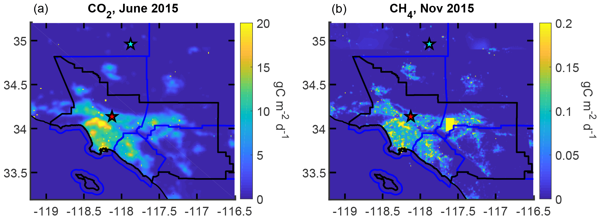
Figure 1A priori flux maps for CO2 (a) and CH4 (b) for select months. The same spatiotemporal prior for CO2 (ODIAC2016) was used for CO, but scaled to 1 % on a per mole basis. The methane prior was created based on point sources, total emissions, and the population distribution. The black lines are coastlines and the geopolitical boundaries of the SoCAB. Blue lines are county borders.
A detailed CH4 inventory is also available for the SoCAB, which we do not use because it would be difficult to scale (Carranza et al., 2018). For the US the Harvard–EPA (Environmental Protection Agency) inventory is already available at resolution (Maasakkers et al., 2016), and globally the EDGAR inventory is available at resolution (EC-JRC/PBL, 2009). We make our own 30 arcsec × 30 arcsec methane prior using landfills, nightlights, expected total emissions, and the US Harvard–EPA inventory (Maasakkers et al., 2016) shown in Fig. 1. Due to a lack of information outside the US on point sources, such as landfills, our methane prior is also not scalable beyond a national level.
For our methane prior we first distribute emissions from landfills as point sources (available 2010–2015, https://ghgdata.epa.gov/ghgp/main.do, last access: 17 August 2017) and use 2015 emissions for 2016. Emissions from the Puente Hills landfill were doubled because the EPA estimate (average of 13.6 Gg CH4 yr−1) is low compared to previous estimates of 34 Gg CH4 yr−1 (Peischl et al., 2013). After doubling Puente Hills emissions, EPA total SoCAB (144 Gg CH4 yr−1) and Olinda Alpha (13.5 Gg CH4 yr−1) landfill emissions are similar enough to other studies (Peischl et al., 2013) that we do not double emissions from other landfills in the SoCAB. Chino dairy emissions were added in as a source (Chen et al., 2016; Viatte et al., 2017). Outside of the SoCAB, CH4 manure and enteric fermentation were added from the Harvard–EPA inventory (Maasakkers et al., 2016). SoCAB emissions are assumed to sum to 400 Gg CH4 yr−1 based on the work of Wunch et al. (2016), and the rest of the emissions were distributed based on population, which was assumed to correspond with the January 2017 Suomi NPP nightlights (15 arcsec). An average monthly trend was included based on results of Wong et al. (2016), and emissions were assumed to be constant on a monthly timescale. Because the Aliso Canyon leak effectively doubled the SoCAB CH4 emissions for its duration from 23 October 2015 to 11 February 2016 (Conley et al., 2016), it was also added as a point source.
We use various publicly available statistics to get a sense of annual CO2 emissions from the SoCAB. Literature estimates range from 99 Tg CO2 yr−1 (Fischer et al., 2017) to 211 Tg CO2 yr−1 (Wunch et al., 2009). Table 1 lists statistics for the SoCAB. We assume the nonresidential natural gas (NG) use is for industry or power already accounted for in the EPA inventory. Because most of the food consumed in the SoCAB is grown outside the basin, such as in the Midwestern US and Central Valley (CV), there is a CO2 return flux to the croplands from both human respiration and food waste. In the US, 60 million metric tons (MMT) of food are lost annually at the retail and consumer levels compared with 129 MMT consumed (Dou et al., 2016), roughly one-third of all food calories (not counting inedible food-related biomass). Presumably, most food waste decomposition would be accounted for in EPA landfill emissions. However, CO2 emissions from food waste could be underestimated if food waste is composted, if there were unaccounted for methanotrophs, or if aerobic respiration is significantly underestimated (e.g., from rapid decomposition while still exposed to oxygen), which would decrease the CH4 : CO2 emission ratio commonly assumed to be unity for managed landfills on a per mole basis (RTI, 2010). Thus, we add 30 % to human respiration emissions of 917 g CO2 d−1 person−1 (Prairie and Duarte, 2007) for food waste losses. We assume the flux from vegetation is balanced (i.e., no net change in plant biomass or soil carbon) within the basin. This choice is because of uncertainty as to whether there is a net uptake of CO2 by the biosphere in the SoCAB (Park et al., 2018) or if the excess CO2 in the atmosphere from the biosphere (Newman et al., 2016) is due to more respiration than photosynthetic uptake. We estimate the uncertainty due to the biosphere is less than ±10 %. Based on these various statistics we estimate a BU net flux of the order of 110 Tg CO2 yr−1 from the SoCAB.
Table 1Statistics for the SoCAB.
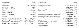
Most of these values are approximations. a https://www.aqmd.gov/nav/about/jurisdiction, last access: 12 November 2018. b http://www.dot.ca.gov/hq/tsip/hpms/datalibrary.php, last access: 12 November 2018. c Assuming 95 % of kilometers light duty vehicles with 9.1 km per liter (KPL) fuel efficiency and 5 % trucks with 2.5 KPL (https://www.fhwa.dot.gov/policyinformation/statistics/2013/, last access: 12 November 2018, VM-1). d Vehicle kilometers and fuel emissions are independent estimates. e http://www.cdtfa.ca.gov/taxes-and-fees/spftrpts.htm, last access: 12 November 2018. f Based on emissions of 1.3×917 g CO2 d−1 person−1 (Prairie and Duarte, 2007). g http://www.ecdms.energy.ca.gov/gasbycounty.aspx, last access: 12 November 2018. h https://www.epa.gov/sites/production/files/2015-07/documents/emission-factors_2014.pdf, last access: 12 November 2018. i Emissions within or near geographical SoCAB boundaries only.
2.3 Dynamical models
A dynamical model is needed in conjunction with the a priori flux estimates to generate forward model Xgas enhancements. Our model uses Lagrangian trajectories driven by existing archived forecast or reanalysis datasets. An advantage of archived model data is there is no need to run a Eulerian model first, and they are more accessible to a broader community. However, taking existing results without model evaluation may propagate hidden errors and biases, which could influence flux results. Archived data usually have coarser spatiotemporal resolutions than custom models and cover larger domains than the area of interest. Custom runs allow models to be parameterized differently and nudged to reduce the measurement–model mismatch for the regions of interest.
We use the North American Mesoscale Forecast System (NAM) at 12 km resolution (3 h temporal) from the NOAA data archive as the primary model source. NAM is run with a non-hydrostatic version of the WRF at its core with a Mellor–Yamada–Janjić planetary boundary layer (PBL) scheme (Coniglio et al., 2013). Estimates of model error are described in Appendix B. Though NAM data are only available over North America, other archived models are available at lower resolution with global coverage (e.g., the Global Data Assimilation System (GDAS) 0.5 ∘, 3 h product). The NOAA ESRL recently began publicly releasing 3 km, 1 h archived data from the High-Resolution Rapid Refresh (HRRR) model that covers the US (Benjamin et al., 2016). This product holds the potential to improve flux estimates at smaller scales.
We use HYSPLIT-4 (Stein et al., 2015) with the three archived NOAA data products described above. Our base method is to use mean 48 h back trajectories with NAM 12 km for the lowest 20 % of the atmosphere, which we assume is the only part of the atmosphere enhanced with local emissions at the measurement site. Trajectories are equally spaced in pressure every 0.3 % of the column. By comparison, the GDAS model takes 0.71±0.18 (1σ) times as long to run, and the HRRR model takes 33.3±7.1 (1σ) times as long. Because HRRR takes substantially longer, we only run it for a subset of months – July and October 2015 and January and April 2016. Other studies (Fischer et al., 2017; Janardanan et al., 2016) used multiple particles released at each level. We assume that over the multiyear time series the ensemble of mean trajectories is, on average, representative of the upwind influences on the receptor sites without the additional turbulence term.
Figure 2 shows back trajectories for one layer that end at the observation sites at 14:00 (UTC−7). Trajectories from multiple vertical levels are combined to determine residence times or footprints as described in Appendix C. There are three major origins for air at the Caltech site. The primary source is from over the ocean and over downtown Los Angeles (southwest). The second major source is from the Mojave Desert (northeast), and the third source is from the CV (northwest; see Fig. E1 in Appendix).
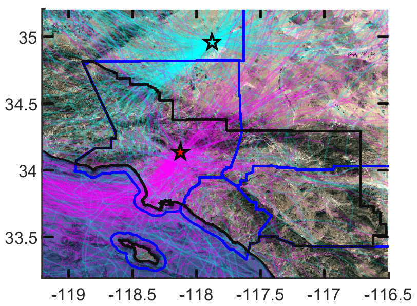
Figure 2HYSPLIT 400 m a.g.l. back trajectories for NAM 12 km for 2015. For each day trajectories are shown ending at the two different TCCON receptor sites at 14:00 (UTC − 7). Magenta trajectories end at Caltech. Cyan trajectories end at AFRC. The black lines are coastlines and the geopolitical boundaries of the SoCAB. Blue lines are county borders.
Others interested in undertaking similar studies may also consider using the recently developed X-STILT (X-Stochastic Time-Inverted Lagrangian Transport) model to obtain footprints for column observations (Wu et al., 2018).
2.4 Inverse methods for comparing measured to model data
Different schemes can be applied to reduce the measured–model mismatch. One of the simplest is to find the ratio between the average enhancements in the observations and the forward model and then to scale the prior based on this ratio. Bayesian inversions are more complex, but can also improve information on the spatial distribution and intensity of fluxes (Lauvaux et al., 2016; Turner et al., 2016); they can be solved by analytical or adjoint methods (Kopacz et al., 2009; Rodgers, 2000). Different cost functions can be used, which might change the results. Here we test and compare three different methods. The first is a Kalman filter (described in Appendix D), which is computationally cheap but has only 1 degree of freedom. For scaling retrievals, using too few degrees of freedom can cause the results to be heavily weighted by the largest model results relative to the observations (Appendix 2). We also use Bayesian inversions based on the methods of Rodgers (2000) (described in Appendix E). One Bayesian inversion is based on a nonlinear forward model with 40 different scaling factors (Eq. E2 in Appendix), and the other is a linear forward model with up to nearly 35 000 scaling factors (Eq. E3), though only a fraction (<1000) of these are used. Because of potential bias in the first two methods, we focus on the linear forward model. Uncertainty estimates are stated for the linear forward model while disregarding the other methods.
2.5 Summary: data sources and methods
In summary, we have four sets of observations of Xgas differences: Caltech TCCON – AFRC TCCON (CO2, CH4, and CO) and OCO-2 – AFRC TCCON (CO2). We use one gridded spatiotemporal inventory for both CO2 and CO (ODIAC2016, with a weekly pattern for hourly emissions), one for sensitivity tests for CO2 (Hestia-LA v2.5) and one gridded spatiotemporal inventory for CH4 (Sect. 2.2). HYSPLIT is run with three dynamical models for the Caltech TCCON – AFRC TCCON differences (GDAS 0.5∘, NAM 12 km, and HRRR 3 km for a subset) and is run with NAM 12 km for the OCO-2 – AFRC TCCON differences. Three different inversion techniques are used, including a Bayesian inversion with a linear forward model, a Bayesian inversion with a nonlinear forward model, and a Kalman filter. Unless specified, values reported are from the Caltech TCCON – AFRC TCCON difference with the NAM 12 km model and the Bayesian inversion with the linear forward model.
Several previous studies have discussed the SoCAB , , and XCO enhancements from local anthropogenic activity (Hedelius et al., 2017a; Janardanan et al., 2016; Kort et al., 2012; Schwandner et al., 2017; Wunch et al., 2009, 2016). There have also been several studies that have discussed enhancements noted from CLARS (California Laboratory for Atmospheric Remote Sensing). CLARS has a viewing geometry that is more sensitive to the mixing layer than TCCON and nadir-viewing satellites, which leads to larger typical enhancements in CO2 and CH4 (Wong et al., 2016, 2015). For comparability we exclude enhancements from CLARS and in situ observations (Verhulst et al., 2017) in this section. Kort et al. (2012) noted that observing changes in typical Xgas enhancements from space-based instruments can provide a first-order estimate of how local emissions have changed year to year without the need for a full inversion. This requires similar year-to-year ventilation patterns and sufficiently large and representative sample sizes, which is becoming less of an issue as more space-based observations become available.
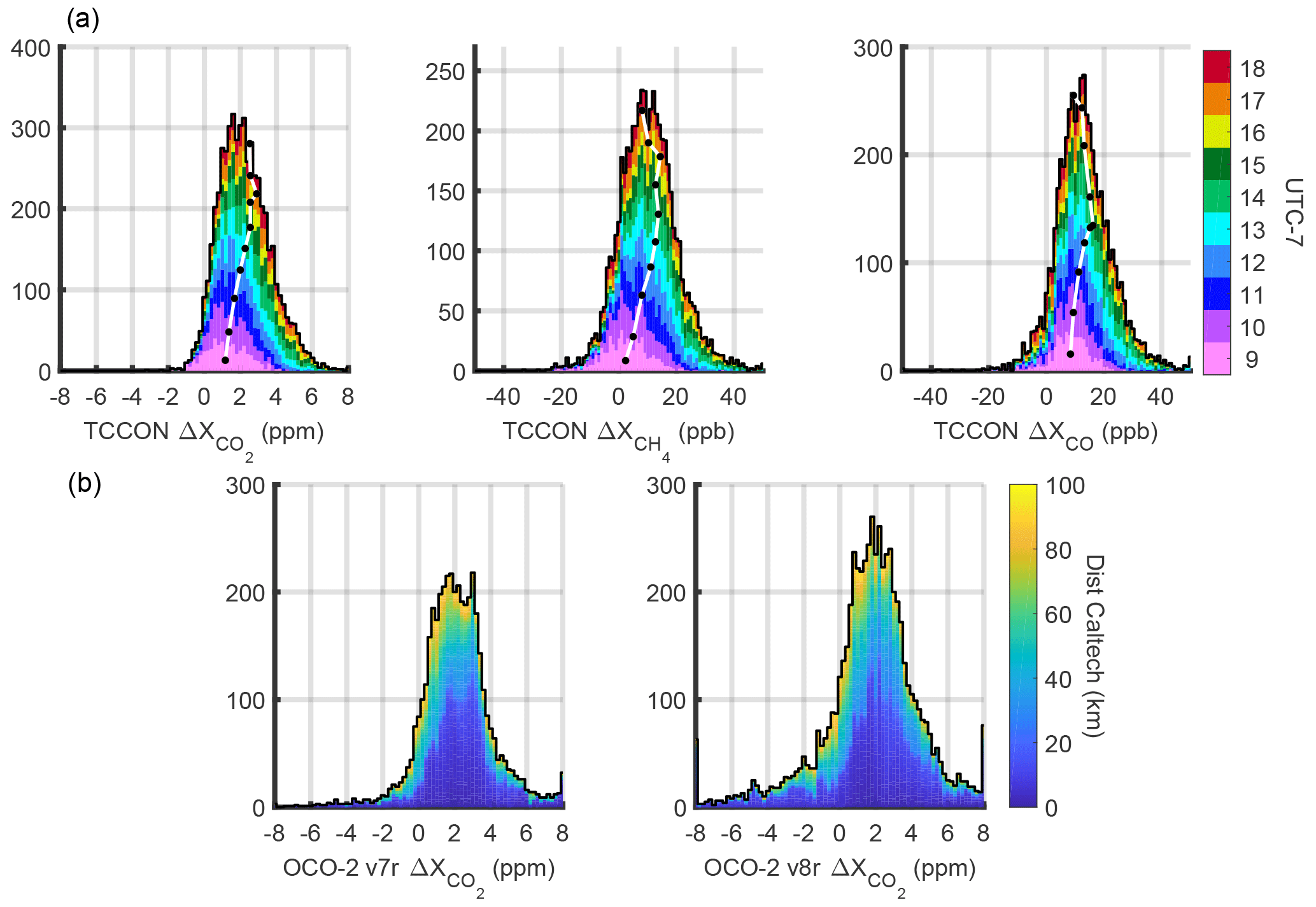
Figure 3Histograms of Xgas enhancements observed in the SoCAB for all dates of this study (Sect. 2.1). Data are averaged for ± 30 min centered on the hour. (a) Enhancements are defined as Caltech TCCON observations minus AFRC TCCON observations (Appendix A). Colors represent the hour of day, and white lines with black dots in the top row are hourly medians. Enhancements peak in early afternoon from morning rush hour emissions being transported from downtown Los Angeles (southwest) to Caltech, and from mixed-layer dynamics. (b) Enhancements are OCO-2 observations minus AFRC TCCON observations. Colors represent the distance from the Caltech TCCON site.
Table 2 lists enhancements observed over the SoCAB compared to an external background. An instrument with a smaller footprint (e.g., OCO-2, about 1.3 km × 2.25 km) could observe a wider range of enhancements than an instrument with a larger footprint (e.g., GOSAT, about 10.5 km diameter). However, the footprint size should not affect the average enhancement over a domain much larger than an individual footprint. Most enhancements in Table 2 are of the order of 2–3 ppm, except for those reported by Schwandner et al. (2017), which are about double. Though their enhancements are within the range of enhancements in the v7r and v8r histograms in Fig. 3b, they are atypical. Their results are likely atypically large because of dynamics on the two particular dates analyzed and do not include enough data to determine typical enhancements, trends, and source and sink attribution. We disagree with their conclusions that these values are in agreement with Kort et al. (2012) and that TCCON validates this high of a typical SoCAB enhancement. Their conclusion that seasonal variations are 1.5–2 ppm does appear to be supported by previous work (Hedelius et al., 2017a). However, their full attribution of the seasonal cycle to biospheric processes within the basin is not supported by the findings of Newman et al. (2016), who found the excess CO2 from the biosphere only varied from 8 % (summer) to 16 % (winter) of fossil fuel excess. More likely the changing enhancement reflects a small change in the biosphere and, most importantly, seasonal differences in the basin ventilation.
Kort et al. (2012)Janardanan et al. (2016)Hakkarainen et al. (2016)Hedelius et al. (2017a)Schwandner et al. (2017)Table 2SoCAB enhancements.
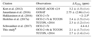
a Qualitative estimate based on Fig. 1 and Supplement Fig. 3 therein. b We modified the boundary condition compared to our previous work (see Appendix A); values are for 14:00 (UTC − 7).
Models that assimilate only global in situ (i.e., no total column) CO2 data are biased by only about ±1 ppm (1σ ∼1 ppm) compared with TCCON observations (Kulawik et al., 2016). This highlights the need to understand bias and uncertainty in total column observations to the order of a few tenths of a part per million or better to provide new information. The TCCON-predicted bias uncertainty is 0.4 ppm or less (<0.1 %). A long-term CO2 reduction goal is to reach 20 % of 1990 levels by 2050. This is about a 2 %–3 % decrease per year assuming a constant reduction. Thus a 0.4 ppm bias is of the order of 4–9 years worth of emission reductions.
4.1 Carbon dioxide
Our flux estimate of CO2 using the TCCON sites and linear model (Eq. E3) is 104±26 TgCO2 yr−1. An error assessment is described in Sect. 4.3. This estimate is shown, along with estimates from past studies, in Fig. 4. Our estimate is lower than those from Vulcan (Brioude et al., 2013; Fischer et al., 2017), Hestia-LA v1.0, Hestia v2.5, and the California Air Resources Board (CARB) 2017. Our result is also slightly lower than those of Ye et al. (2017), who estimated emissions by comparing OCO-2 observations with forward model results from a WRF-Chem model. Our result differs significantly from previous TD estimates from aircraft flights, EDGAR v4.0 (Wunch et al., 2009), and CARB 2011. Between 2011 and 2012 CARB changed how bunker fuels and aircraft emissions were reported for the state, which caused a significant decrease in reported emissions. Our posterior estimate is similar to that of EDGAR v4.2 and ODIAC2016, which is slightly less than ODIAC2015. The ODIAC2016 is based on disaggregation of CDIAC national total emissions. Thus, unlike locally developed emission inventories the interannual variations in subnational emissions are driven by the national emission trends. ODIAC could be low from incorrectly distributing too much of the emissions to rural areas due to blooming effects (Small et al., 2005). Blooming effects refer to the tendency for nightlights to exaggerate settlement areas compared with actual extent due to coarse gridded spatial resolution and indirect or nonelectrical light.
Most of the estimates from previous studies include only emissions from fossil fuel use. We have not separately accounted for biospheric uptake (emissions) in the model, and if it is significant, the anthropogenic flux would be larger (smaller) than our net estimate. In the GEOS-Chem model described by Liu et al. (2017) the nearby ocean is a neutral to weak sink, likely from biological activity.
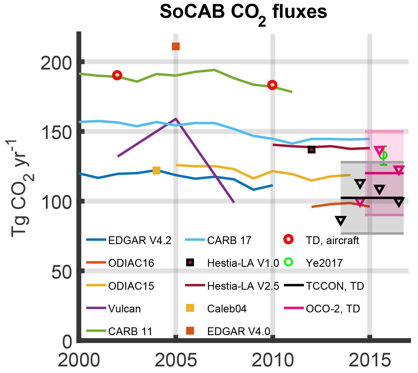
Figure 4Estimates of SoCAB CO2 fluxes (annual estimates from TCCON are shown as black triangles and OCO-2 estimates are shown in pink) compared with previous studies. TD aircraft estimates are from Brioude et al. (2013). TD estimate from Ye et al. (2017) is based on OCO-2 observations and 5 % random uncertainty has been added. The Hestia-LA v1.0 estimate was inferred after a forward implementation into a WRF model (Hedelius et al., 2017a). EDGAR v4.2, ODIAC, and CARB emissions were calculated from databases. The EDGAR v4.0 value was reported by Wunch et al. (2009). All other values were found in a literature review. The large range of variability highlights the need for additional study of SoCAB CO2 fluxes.
OCO-2 provides better spatial coverage than TCCON (Fig. 5), and the orbit tracks can change longitudinally with season or when the spacecraft moves for collision avoidance. However, observations only occur at the same local solar time, and are days to weeks apart. The estimate using OCO-2 data is slightly larger at 120±30 TgCO2 yr−1, which is in better agreement with the results of Ye et al. (2017). This value varies by up to 12 TgCO2 yr−1 depending on filtering methods (e.g., warn levels, Appendix 1).
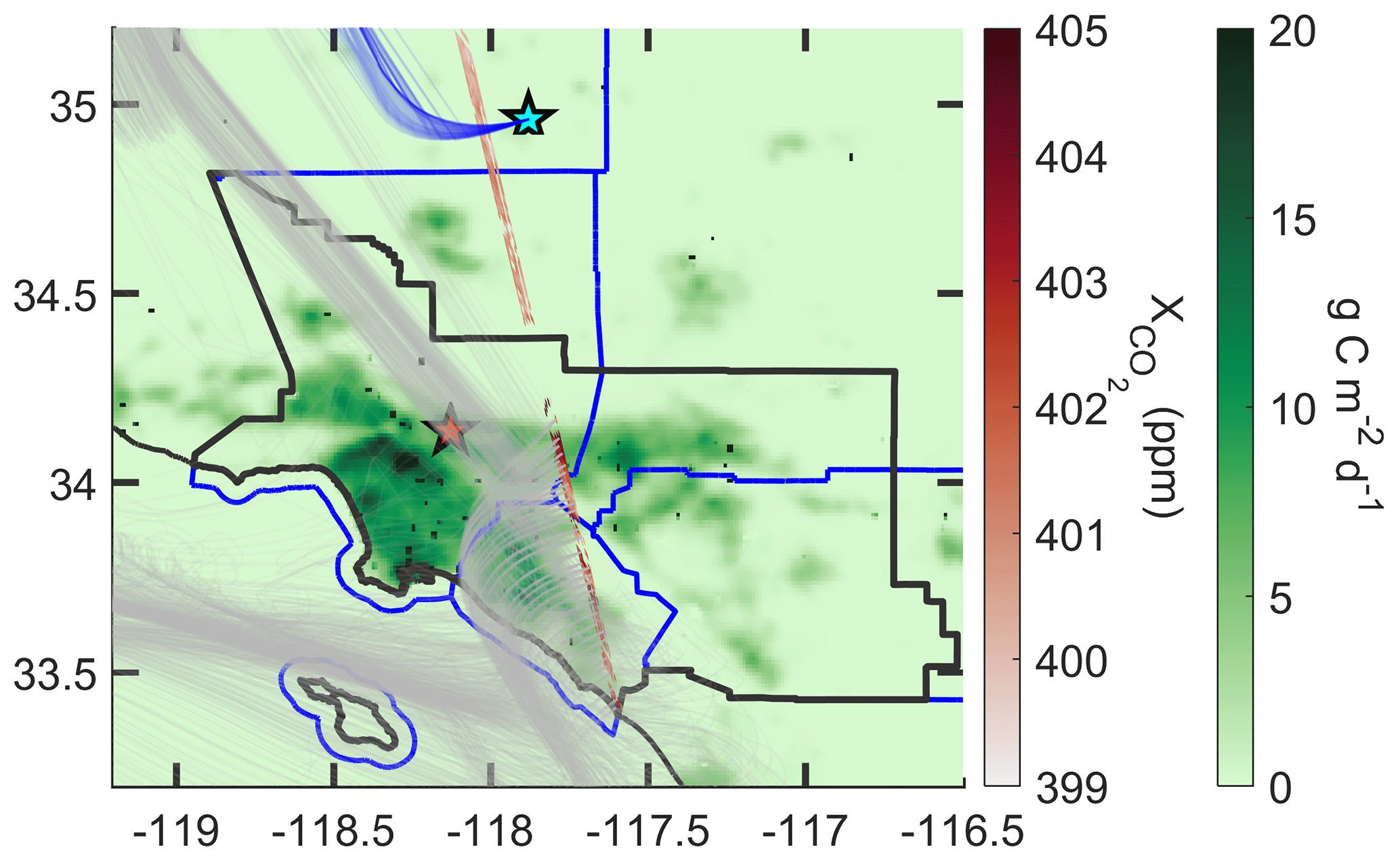
Figure 5A visualization of OCO-2 observations and the forward model used in the flux inversion on 20 June 2015. The nadir track is shown in red starting at the bottom and and going towards the northwest. Observations are overlaid on the green ODIAC prior at 14:00 (UTC − 7). For every fifth sounding the set of back trajectories is shown in gray. Back trajectories originating from the AFRC site are shown in blue. Coastlines and the geopolitical boundaries of the SoCAB are shown in black. County borders are shown in blue.
4.2 CH4 and CO
Using the same methodology we estimate a CH4 flux of 360±90 Gg CH4 yr−1. This is less than the estimate by Wunch et al. (2009) but similar to estimates from Wong et al. (2016) and CARB (Fig. 6). CARB-based CH4 fluxes for just the SoCAB were estimated by subtracting agriculture and forest emissions (53 %–61 % of total depending on version and year) and out-of-state electricity generation (0 %–0.1 %). The remaining flux was scaled by 42 % based on the population of the SoCAB, and 5 % of the agriculture and forestry emissions were added back in. Our estimate is slightly lower than previous estimates of CH4 fluxes using in situ (tower and aircraft) data (Cui et al., 2015; Hsu et al., 2010; Peischl et al., 2013; Wecht et al., 2014; Wennberg et al., 2012).
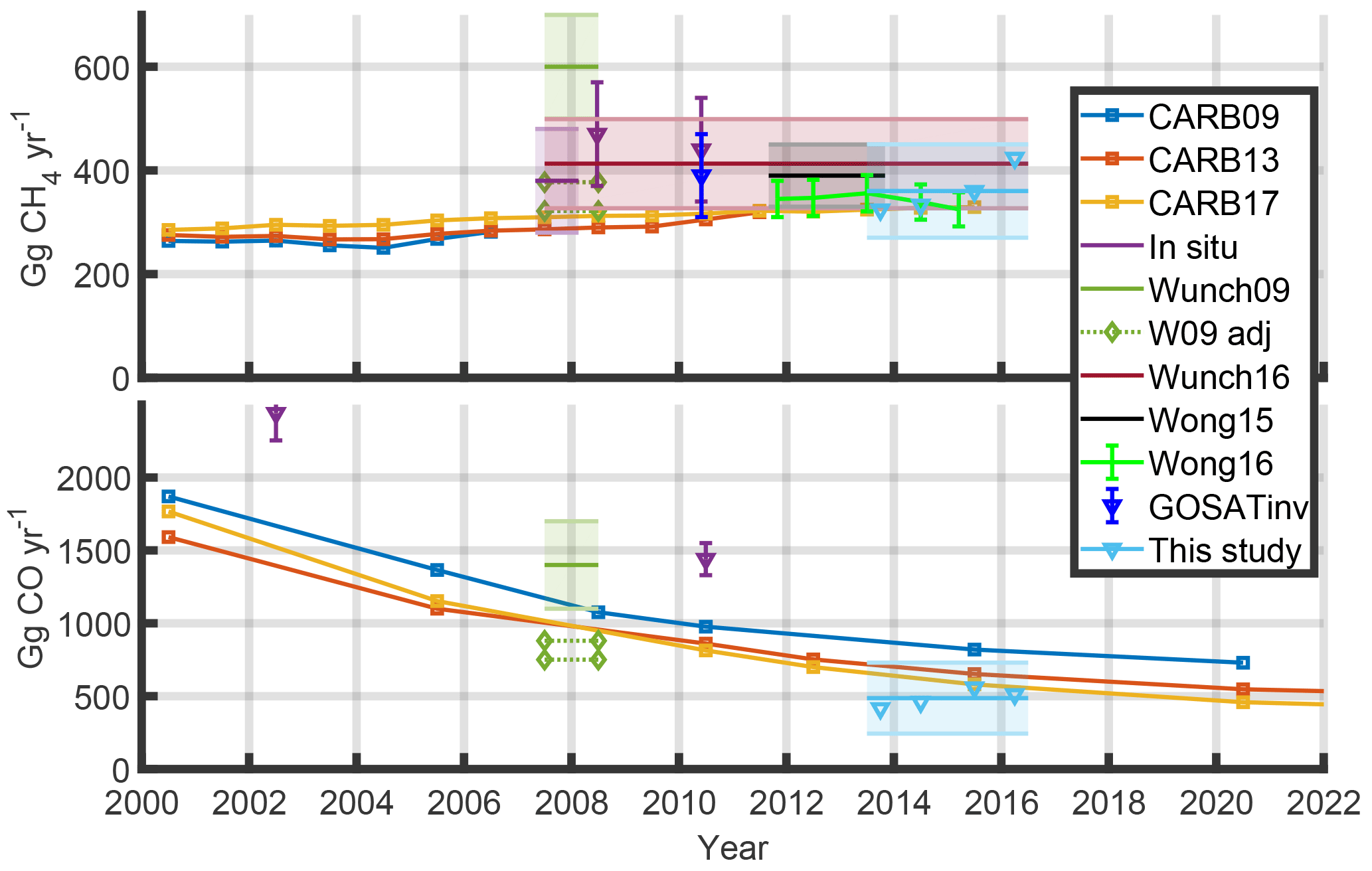
Figure 6SoCAB CH4 and CO flux estimates. Annual estimates from this study are shown as light blue triangles. Brioude et al. (2013) and Wecht et al. (2014) (in situ estimates and GOSAT inv) used meteorological models to estimate fluxes, similar to the work presented here. Tracer–tracer relations were used for the TCCON (Wunch et al., 2009, 2016), CLARS (Wong et al., 2016, 2015), and in situ observations (Hsu et al., 2010; Wennberg et al., 2012). “W09 adj” shows the results of Wunch et al. (2009) when adjusted for our posterior CO2 flux. Methane in situ results for CalNex (May–June 2010) are from Wennberg et al. (2012). CO in situ results in 2002 and 2010 are from Brioude et al. (2013).
We also estimate a CO flux of 487±122 Gg CO yr−1. This is significantly less than the estimates by Wunch et al. (2009) of 1400±300 Gg CO yr−1 from August 2007 to June 2008 and the estimate of 1440±110 Gg CO yr−1 by Brioude et al. (2013) for summer 2010. Wunch et al. (2009) used a tracer–tracer relationship in which the assumed CO2 was likely too large (191 TgCO2 yr−1). When their results are scaled down based on our posterior CO2 fluxes (104–120 TgCO2 yr−1), the CO flux is 750–880 Gg CO yr−1, which is in better agreement with the CARB inventory. The CARB CO inventories, specific to the SoCAB, have decreasing CO emissions; part of the difference could be from different observation periods. CARB2017 emissions are 581 Gg CO yr−1 for 2015.
4.3 Sensitivity tests and error assessment
For a single estimate of the SoCAB flux, we have a sufficiently large sample that random uncertainty is small. This is supported by a bootstrap analysis in which we select a random subset of data equal in size to the original n=200 times (Efron and Gong, 1983). The random uncertainty estimate is 4 Tg CO2 yr−1 (2σ), or about 4 %. Persistent biases from a priori flux uncertainty, model errors, observation biases including boundary conditions, and poorly chosen initial values are more detrimental to our flux estimate.
Several variables (xa, Sϵ, Sa) need initial values (see Appendix 3), and how these are chosen can affect the final flux calculated. We evaluate four sensitivity tests (Fig. 7). For the first test, we filter out data for which the observations differ from the model above a threshold. We scale from the starting factor of 10× (Appendix 1). We also adjust values of xa, Sϵ, and Sa by factors of 2−10 to 210. These results show the overall flux generally has low sensitivity to scaling Sϵ and Sa but has some sensitivity when filtering more data and about a 30 % sensitivity to the scaling of xa. The interannual variability, which we expect is less than about 25 %, increases for large Sa. Increasing Sa increases r and the degrees of freedom for the signal (dofs) with only a small effect on the overall flux but also increases the interannual range. Decreasing Sϵ increases r and dofs, but it also increases χ2 and the interannual range. We estimate an overall uncertainty of 10 % from these parameters.
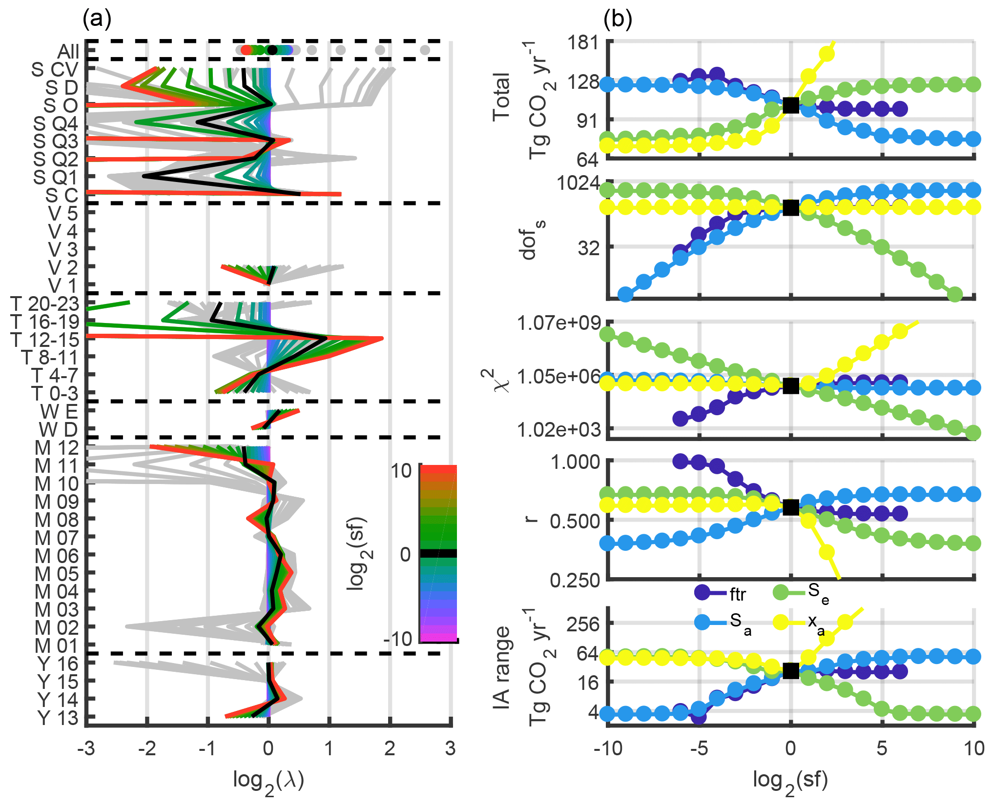
Figure 7Assessment of sensitivity to initial values for CO2. (a) Reduced state vector with seven categories (overall, spatial, vertical, time of day, weekday–weekend, month, and year). λ values indicate how much the prior is scaled on average compared to other elements in its category. Gray lines are results from all tests, and colored lines are from the Sa test. As Sa gets larger, the variability in the retrieved γ factors increases. Missing elements represent lack of sensitivity. (b) Overall fit parameters, including the overall flux, dofs, χ2, Pearson's correlation coefficient between observed and post-inversion model values, and the interannual range. Note the log2 axes, which indicate the magnitude of change in the sensitivity test compared with the base case (sf: scaling factor). Moving left, filtering (ftr) becomes more stringent, constraints on Sa or Se are increased, or xa is scaled down. For scalings less than about 8× the total flux change is small, except for scaling xa, which increases the flux by about 30 % of the change in the prior. Here the goal was to simultaneously increase dofs, decrease χ2, and increase r while keeping the interannual variability below about 25 %.
We next test the sensitivity to different inversion and modeling schemes (Table 3). The Kalman filter (Appendix D) and the nonlinear inversion (Eq. E2) results are not unreasonable for CO2. However, their CH4 flux results are unreasonably low, likely from high model : measured values having unreasonably high weights in these particular schemes with few scaling factors (Appendix 2). GDAS and HRRR results are within uncertainty.
Table 3Fluxes from various methods.
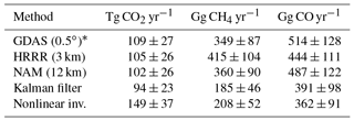
For a given gas, all the inversions use the same observed ΔXgas (Caltech TCCON − AFRC TCCON) data. The top three rows are from using different meteorological models, with the same inversion scheme (Eq. E3). The last three rows are from using the same meteorological model (NAM 12 km) with different inversion schemes. Errors are 25 %. * For GDAS Sa is 20× smaller.
There is some uncertainty due to the accuracy and resolution of the emission inventories. Gately and Hutyra (2017) compared emission inventories over the northeastern US and noted inventory differences of 100 % for half of the 0.1∘ grid cells in the domain. Lauvaux et al. (2016) and Oda et al. (2017) compared aggregate posteriori inversion results from different emission inventories and noted differences of only 5 %–8 % for the Indianapolis region despite large differences at the grid level. We make a similar comparison in which we use the more spatially and temporally accurate Hestia v2.5 fossil fuel inventory instead of ODIAC as the prior. We note that the correlation between the forward model data and TCCON is slightly higher with Hestia than ODIAC, and there are fewer outliers that differ by a factor of 10× or more. However, the flux estimate of 110±28 is similar to the posterior flux estimate using ODIAC.
Finally we consider the observation uncertainty. Hedelius et al. (2017b) reported a 2σ measurement bias of less than ∼0.2 ppm (central estimate, maximum range <0.5 ppm) between the AFRC and Caltech TCCON sites, but even a bias of 0.2–0.3 ppm will produce an error of ∼ 10 % in the flux. This bias could also arise from improper boundary conditions or application of averaging kernels.
In summary, we estimate 5 % random uncertainty from the bootstrap analysis, 10 % from our choice of initial values, 5 % from the prior flux, 10 % from observations and the boundary condition, and 20 % from model winds (Appendix B). The sum in quadrature is 25 %. By comparison, uncertainty estimates from other inversions were 11 % (inner 50 percentile range from an ensemble) for Indianapolis (Lauvaux et al., 2016) and 5 % for the Bay Area using pseudo-observations (Turner et al., 2016). Both of these studies benefited from additional sites (nine and 34, respectively) and custom WRF model runs. Ye et al. (2017) estimated an uncertainty of 5 % for the SoCAB flux by using data from 10 OCO-2 tracks; however this is not directly comparable with our result because it does not include uncertainty from biases in the forward model, observations, and inversion scheme.
5.1 Emission ratios
Emission ratios can help us evaluate the inversion for the SoCAB. In previous studies it was noted that the Pasadena area is a good receptor site for the basin, so tracer–tracer ratios observed there should approximately correlate with emission ratios (Newman et al., 2016; Wunch et al., 2009, 2016). If the ratios are significantly different it could highlight an error in the inversion scheme or the a priori assumption of sources. However, errors in the model can be correlated for different tracers, which would obscure universal biases to all gases. For example, the CO : CO2 flux ratio of 7.5 ppb : ppm is in good agreement with past literature, despite the absolute fluxes being lower on average.
We estimate emission ratios using the solar zenith angle (SZA) anomaly method described by Wunch et al. (2009, 2016) and using the average enhancement compared with AFRC or the Pasadena : Lancaster gradient ratio. Errors are assumed to equal the standard deviation of all the data, and a linear fit is made using the methods of York et al. (2004) on monthly timescales. We estimate the emission ratio from the work of Verhulst et al. (2017) using the weighted mean of the excess ratios from their five in-basin sites, with weights of . Emission ratios from the SZA anomaly method and the differenced enhancement are in agreement with ratios from previous studies (Fig. 8). The CH4 : CO2 from the inversion at 9.7 ppb : ppm is larger than past studies, suggesting either our CH4 flux is too large or our CO2 flux is too low (or some combination of both). If both were adjusted by 15 % the ratio would be 7.1 ppb : ppm. The CO : CO2 ratio is in good agreement with the ratios using the SZA anomaly method, but is lower than past estimates. Based on the CARB inventories, a decrease is expected because CO emissions have decreased almost exponentially over the past decades, whereas CO2 emissions have decreased only moderately (e.g., compare Figs. 4 and 6).
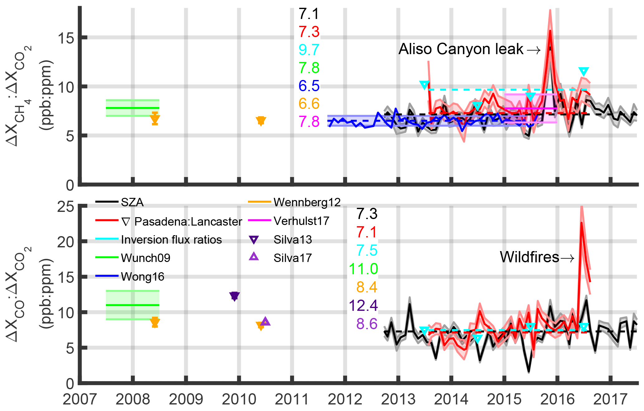
Figure 8Emission ratios compared with previous studies. Numbers shown are central values from the different methods and studies. Overall fits are shown as dashed lines. The ratio from the gradients of Pasadena (Caltech) to Lancaster (AFRC) is based on the difference between the two TCCON sites. Values from Silva et al. (2013) and Silva and Arellano (2017) were part of global studies.
In November 2015, the large CH4 : CO2 ratio is from additional methane emissions from the Aliso Canyon gas leak (Conley et al., 2016). Though this leak persisted until February 2016, different wind patterns caused less of the highly methane-enriched air to be transported and observed in Pasadena after the first 2 months. The large CO : CO2 ratios seen in summer 2016 are from wildfires. The San Gabriel Complex Fire was less than 25 km to the east and burned 22 km2 over a month. It was close enough for ash to be transported to Pasadena. Eight other major fires within 150 km burned an additional 400 km2 during June–August 2016 (http://cdfdata.fire.ca.gov/incidents/incidents_archived?archive_year=2016, last access: 12 November 2018).
Pollack et al. (2012)Brioude et al. (2013)Table 4Weekday : weekend emission ratios.
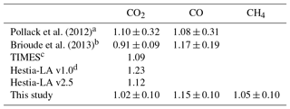
a WD : WE CO ratios from Pollack et al. (2012) were calculated using the difference between the CalNex-Pasadena and c Flasks (Table 2 therein). For CO2 we used the CO WD : WE ratios with the CO : CO2 WD : WE ratios in Pasadena (Table 3 therein). b WD : WE ratios from Brioude et al. (2013) were calculated by assuming ratios between daytime and all-day emissions in the posterior were equal using Table 3 therein. c Temporal Improvements for Modeling Emissions by Scaling (TIMES) were reported for the contiguous United States by Nassar et al. (2013). d Hestia-LA is based on Fig. 2 from Hedelius et al. (2017a). This same ratio is used in the CO and CO2 priors in this study.
5.2 Weekend effect
The weekday-to-weekend (WD : WE) flux ratios are listed in Table 4. The uncertainty is estimated to be ±0.10 based on changes in the ratio from the Sa scaling test up to 16× (Fig. 7). Weekday : weekend ratios are similar to those from previous studies for CO (Brioude et al., 2013; Pollack et al., 2012). The CO2 and CO ratios are scaled down compared with the prior, which puts CO in better agreement with Hestia-LA v2.5. Methane has a ratio that is slightly larger than unity. Methane is not expected to vary as much as CO2 or CO on weekdays compared to weekends because production from biogenic sources and fugitive losses from natural gas infrastructure are less time variant.
This study demonstrates a method to readily obtain estimates of net CO2 fluxes over regions of the order of 10 000 km using remote-sensing observations. This work is a step towards estimating fluxes from a greater number of urban areas using space-based observations of CO2. Our estimates of total annual CO2 fluxes from the SoCAB using HYSPLIT with NAM 12 km as our dynamical model are on the low end of previous estimates (Fig. 4) and about 28 %–47 % less than inventory values reported in tracer–tracer flux estimate papers (Wong et al., 2015; Wunch et al., 2009). This has important implications for these studies, which would have overestimated CH4 emissions if CO2 emissions were also too large. Net CO fluxes are significantly less than previous studies, likely from an underestimate of about 20 % combined with a known decrease in emissions. Net CH4 fluxes are in agreement with previous studies.
This study is one of only a few in which satellite observations were used to help infer the net flux of CO2 from an urban area. Several lessons learned here will be important for future studies using space-based observations of CO2 for flux estimates from other urban regions. We have shown a method for accounting for the sensitivity of the instrument to true changes in the atmospheric composition (i.e., accounting for averaging kernels). We have also shown a method to account for differences in column observations that could arise from different surface altitudes. In the Appendix we document how changing the number of elements in a retrieval state vector can, in some cases, bias the inferred flux result. This effect becomes increasingly important for inversions using only one scale factor with a large discrepancy between the forward model and observations. Finally, we describe the sensitivity of the results to filtering and parameters such as the a priori and the a priori covariance matrix Sa.
The overall uncertainty is 25 %, with the dynamical model contributing the most. X-STILT (Wu et al., 2018) and higher-resolution models (e.g., HRRR) may help reduce dynamical model uncertainty in future inversions. We consider an uncertainty of 25 % to be large and it shows additional work is needed to improve constraints. If errors are from persistent biases, then relative changes in time can be observed, though such changes might also be observed using just the observations without a model (Kort et al., 2012). Understanding contributions from the biosphere may also be important in future studies to diagnose how much carbon is from fossil fuels (Newman et al., 2016). The wide range of uncertainty suggests that CO2 flux estimates from the SoCAB will benefit from additional measurements – such as the LA Megacity Carbon Project in situ tower network (Verhulst et al., 2017), the planned geostationary GeoCARB mission, and the OCO-3 mission, which has a raster mode that can scan throughout the basin. Further improvements in modeling and inversion techniques will also help, including assimilating all available observations (in situ network, TCCON, CLARS, OCO-2, and GOSAT). These additional surface and space-based observations can not only aid in improving the accuracy of the overall flux, but also may be incorporated into spatiotemporal inversions to map fluxes from subregions of the SoCAB with confidence.
TCCON data used in this study (GGG2014: Iraci, et al., 2014; Wennberg et al., 2014) are hosted at the TCCON data archive (https://tccondata.org/, last access: 23 November 2017) and are used in accordance with the Data Use Policy (https://tccon-wiki.caltech.edu/Network_Policy/Data_Use_Policy, last access: 23 November 2017). OCO-2 data (OCO-2 Science Team et al., 2017) are hosted by Goddard Earth Sciences (GES) Data and Information Services Center (DISC) (https://disc.gsfc.nasa.gov/datasets/OCO2_L2_Lite_FP_8r/summary, last access: 2 January 2018). ODIAC2016 data (Oda et al., 2015) are hosted by NIES (http://db.cger.nies.go.jp/dataset/ODIAC/, last access: 30 July 2018). Hestia-LA and Vulcan data can be obtained by contacting Kevin Gurney (Kevin.Gurney@nau.edu). Nightlight products were obtained from the Earth Observation Group, NOAA National Geophysical Data Center and are based on Suomi NPP satellite observations (http://ngdc.noaa.gov/eog/viirs/, last access: 16 August 2017). Gridded Harvard–EPA emissions are hosted on the EPA website (https://www.epa.gov/ghgemissions/gridded-2012-methane-emissions, last access: 10 November 2016). NOAA gridded meteorological data are hosted on the NOAA ARL server (https://www.ready.noaa.gov/archives.php, last access 24 October 2017). The CARB regularly publishes emission inventories of various gases. CO inventories are available online (2017: https://www.arb.ca.gov/app/emsinv/2017/emssumcat.php, 2013: https://www.arb.ca.gov/app/emsinv/2013/emssumcat.php, 2009: https://www.arb.ca.gov/app/emsinv/fcemssumcat2009.php, last access: 12 November 2018), as are CH4 inventories (2017: https://www.arb.ca.gov/app/ghg/2000_2015/ghg_sector_data.php, 2013: https://www.arb.ca.gov/app/ghg/2000_2011/ghg_sector_data.php, 2009: https://www.arb.ca.gov/app/ghg/2000_2006/ghg_sector.php, last access: 12 November 2018).
GOSAT–ACOS v2.9 levels are enhanced by only 3.2 ± 1.5 (1σ) ppm in the SoCAB (Kort et al., 2012). This means a bias of 0.3 ppm could lead to a 10 % bias in the flux. Thus it is critical to account for biases down to the tenths of a part per million level or better. This is a challenge given that the accuracy of OCO-2 (v7r) over land had been estimated as 0.65 ppm (Worden et al., 2017), and OCO-2 comparisons with TCCON range from −0.1 to 1.6 ppm (Wunch et al., 2017).
A1 Quality filters
Compared with the TCCON, OCO-2 spectra have a lower resolution. OCO-2 observations are also sensitive to surface albedo and are more sensitive to aerosol scattering than solar-viewing instruments. These sensitivities can cause spurious results, which need to be filtered out. Included in the OCO-2 data is a binary flag as well as warn levels (WLs) for quality filtering. WLs are a global metric of data quality, for which WLs less than or equal to (0, 1, 2, 3, 4, 5) correspond to about (50 %, 60 %, 70 %, 80 %, 90 %, 100 %) of data passing in v8r, and larger WLs generally correspond to less reliable data. WL definitions are different for v7 and v8, but here we use the binary filter and only include v8 data with a WL ≤1. WL ≥4 data are already removed by the binary flag. We also exclude data that differ from the model by a factor of 10 or more. This factor of 10 is somewhat arbitrary and an argument could be made against using this criterion as a filter. However, a few large outliers can significantly affect inversion results (Appendix 2) so we opt to remove suspect values. A sensitivity test including different filter cutoffs for TCCON is described in Sect. 4.3. After filtering, 2361 paired OCO-2–AFRC observations remain.
For TCCON observations we use the public data, which already have some static within-range filters applied. We also exclude data that differ from the model by a factor of 10 or greater, leaving 4872 observations.
A2 Background, boundary conditions, and averaging kernels
To eliminate the ambient Xgas levels that would be observed in the absence of local emissions, we subtract values measured by the AFRC TCCON site from both the Caltech TCCON and OCO-2 data obtained in the basin. We choose TCCON data as background for OCO-2 to reduce the likelihood of albedo-related bias from using OCO-2 observations over the Mojave Desert (Wunch et al., 2017) as well as the chance of inducing a bias from using different viewing modes by using ocean glint observations. In other studies of enhancements, observations not directly influenced by the source were used as background. For example, Janardanan et al. (2016) categorized space-based observations of by making a forward model estimate of enhancements from fossil fuel combustion and setting a threshold to define as polluted or unpolluted. Such an approach could work globally but may have errors from the prior emissions or transport model.
Because we expect most of the difference in to arise from polluted air near the surface, we divide the enhancements by the surface averaging kernels of the in-basin observations. OCO-2 surface averaging kernels in the basin are 0.986 ± 0.010 (1σ) with a 99 % confidence interval of 0.955 to 1.016. TCCON surface averaging kernels depend on surface pressure and solar zenith angle (SZA) and are 0.96 ± 0.14 (1σ) throughout the full range of observations.
Even in the absence of local anthropogenic emissions, the measured within the SoCAB could be different from that measured at AFRC by a few tenths of a part per million because of different measurement heights and atmospheric CO2 profiles (Hedelius et al., 2017a). We account for a boundary condition of the form
where subscript “a” represents the a priori estimate, S represents a measurement within the SoCAB, B represents the background, and the circumflex represents a retrieved value. Equation (A1) can be interpreted as the difference that would be observed between two sites due to differences in the gas vertical profiles. The a priori profiles do not include local anthropogenic emissions. The result from Eq. (A1) is subtracted from the SoCAB–AFRC difference. We perform the same adjustment for CH4 and CO.
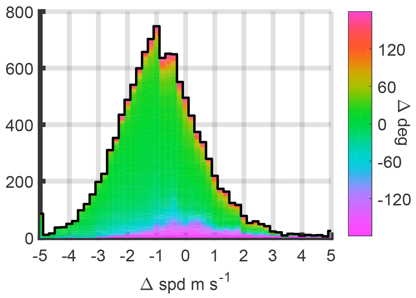
Figure B1Histogram of wind speed errors (HYSPLIT minus measured) compared to surface observations at the San Gabriel airport. The mean error is −0.9 m s−1 (−30 %), the 95 % confidence interval is [−3.7, 2.3] m s−1. The mean direction error is less than 5∘, and 75 % of direction errors are within .
Dynamical models can have errors in the PBL height estimation as well as in the wind speed and direction. In a case study for spring 2011 and 2012 primarily over the Midwestern US, a NAM temperature-derived PBL height had a mean bias of about −50 m, with an inner 50 percentile range of about ±250 m (Coniglio et al., 2013). For wind error we compare with 10 m winds from the San Gabriel (El Monte) Airport 10 km SE of Caltech (lat 34.083, long −118.033, 90 m a.s.l.). We assume the winds are the same at both locations. Airport meteorological data are obtained through the NOAA National Centers for Environmental Information (https://www.ncdc.noaa.gov/cdo-web/datatools/lcd, last access: 12 November 2018).
Trajectory speed and direction are estimated based on when and where trajectories ending at 50 m a.g.l. enter a 5 km radius circle around the receptor site. Results are shown in Fig. B1. The mean speed of HYSPLIT trajectories is less than what is expected by comparing with the surface winds. In contrast, previous studies have shown high model wind speed bias near the surface at the LAX airport, 34 km to the southwest, and near the coast (Angevine et al., 2012; Feng et al., 2016; Ye et al., 2017). The difference biases could in part be from the coast versus inland; however, Feng et al. (2016) also showed a high model bias closer to Caltech. Model differences, the 10 km horizontal and ∼150 m height difference between Caltech and the airport could also contribute to the discrepancy. We expect the average bias throughout the PBL to be lower than at the surface and assign an uncertainty of up to ∼20 % to the average wind.
HYSPLIT mean trajectories are air parcel locations at different heights for select times (in our case, every 20 min). These are aggregated and normalized for each 0.01∘ × 0.01∘ cell and for each hour. First each trajectory is interpolated to 1 s positions. Then we determine the vertical fraction of the mixing layer the trajectory takes. This fraction is the ending vertical spacing between adjacent trajectories (hPa) divided by the local mixing-layer depth (hPa). The HYSPLIT mixing depth is based on the underlying Eulerian model. Parcels above the mixing layer get counted as zero. Then we count how long any parcel was in each cell (s) to obtain the residence time. Monthly average examples of this are shown in Fig. C1. The residence time is multiplied by the a priori flux to determine the column enhancement (g m−2). By dividing by a model estimate of the dry air (molecules m−2) based on model surface pressure, we obtain a forward model estimate of the Xgas enhancement from local sources (ppm or ppb).
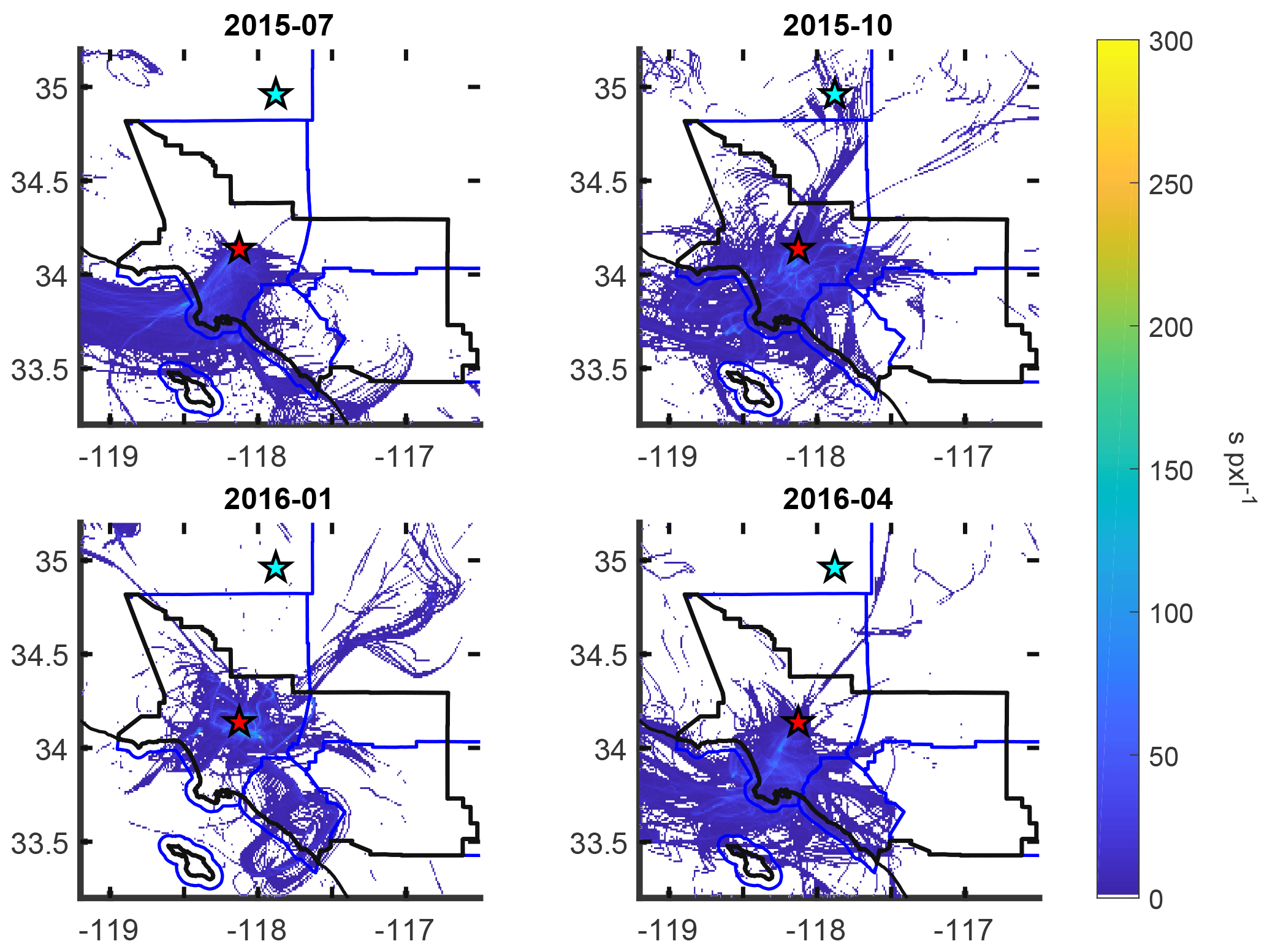
Figure C1Maps of monthly averaged residence times in the mixing layer per pixel for trajectories ending at 21:00 UTC, shown for all times leading up to the observation. Pixels are , or approximately 1.03 km2. In July the origins were more predictable, but in January there was greater variation. Coastlines and the geopolitical boundaries of the SoCAB are shown in black. County borders are shown in blue.
The Kalman filter used to estimate SoCAB CO2 emissions is based on methods described by Kleiman and Prinn (2000) with modifications. This is an iterative approach using a single overall scaling factor. The difference in between measurements in the SoCAB and AFRC is the observed measurement, yobs. The error σy associated with each yobs is estimated from the sum in quadrature of the error from each site, i.e.,
where the subscript C is for Caltech (or measurements in the SoCAB), and A is for AFRC (or “background”). The error of the averaged data for an individual site is estimated as
where n is the number of measurements, are the individual measurements, are the reported errors associated with the measurements, and is the weighted average using as weights. Note that Eq. (D2) takes into account both the measurement errors and the spread of the measurements. However, we note that a similar equation underestimated the error compared with a bootstrap method (Gatz and Smith, 1995).
D1 Iterations
We initialize the iterations with an arbitrary scaling factor α0=1 and an associated error of σα 0=0.7. These initial values have little influence on the final result.
We iterate over the k measurements by calculating the partial derivative:
where subscript j is for a particular grid box, s is the a priori surface flux, and t is the residence time. Equation (D3) is identical to Eq. A2 in Kleiman and Prinn (2000). Because this is a scaling retrieval, hk is the observation operator. We can multiply it by the state element (α) to obtain the estimated observation (Eq. D6). The gain scalar gk and new state error are calculated by (Eqs. A4 and A5 in Kleiman and Prinn, 2000)
We make a modification to calculate the estimated measurement, omitting the term for the convergence of fluxes due to unresolved motions in the transport model. The estimated forward model is
and the state estimate is
D2 A note on single scale factor inversions with large outliers
Some single scale factor inversions can be written in the form
where “mod” represents the initial model values. We consider the case when cost function is of the form
where the error term accounts for both the model and observation errors. If the error is not a function of λ then
Setting Eq. (D10) equal to zero and solving for λ yields
Note the change from vector to summation notation. Equation (D11) is a first-order estimate of the overall scale factor λ. This indicates that λ can be low with high model : observation ratios, which heavily weight the result.
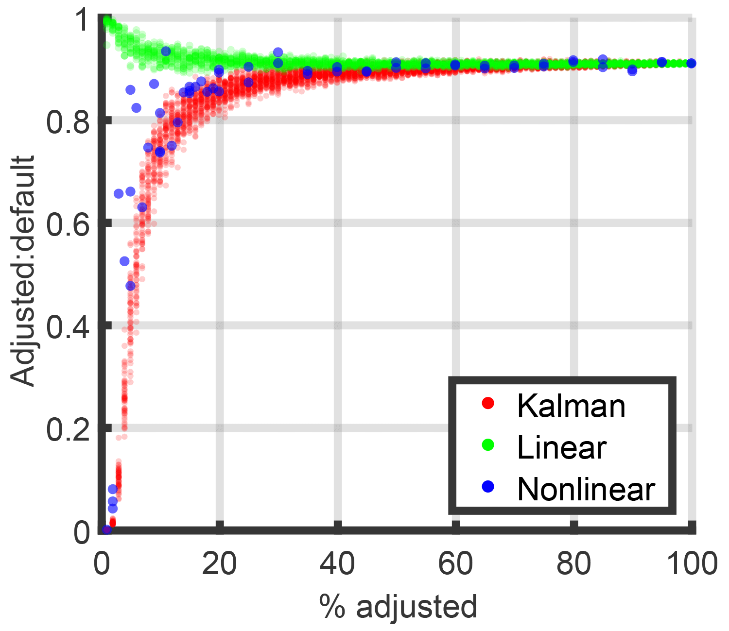
Figure D1Effects of scaling a random subset of model data compared to no scaling. When fewer points are scaled, they are scaled by a larger amount. The Kalman filter and nonlinear inversion are more affected by a few strong outliers than the linear inversion.
This is demonstrated in a sensitivity test, in which we scale a subset of points (Fig. D1). We create pseudo-observed values by using the original model values. We create pseudo-model data by scaling a random subset of the original model data by , for which n is the total number of points, and s is the number in the subset. For example, when 100 % of the model points are adjusted we scale them all up by 10 %. The test is repeated multiple times, with fewer repeats for the nonlinear model because it takes the longest. These results show that having a few large outliers in the Kalman filter (one scale factor) and the nonlinear (40 scale factors, Sect. E) inversions can significantly pull the results compared with the linear (∼1000 scale factors, Sect. E) inversion.
The Bayesian approach to solving atmospheric inverse problems has been described in more detail by Rodgers (2000). Turner et al. (2016) describes this approach for an urban region. Here we follow the notation of Rodgers (2000). For scaling retrievals, Bayesian inversions minimizes a cost function () of the form in Eq. (D9). This assumes error statistics are adequately known and are Gaussian for both the state vector x (length n) and the measurement vector y (length m).
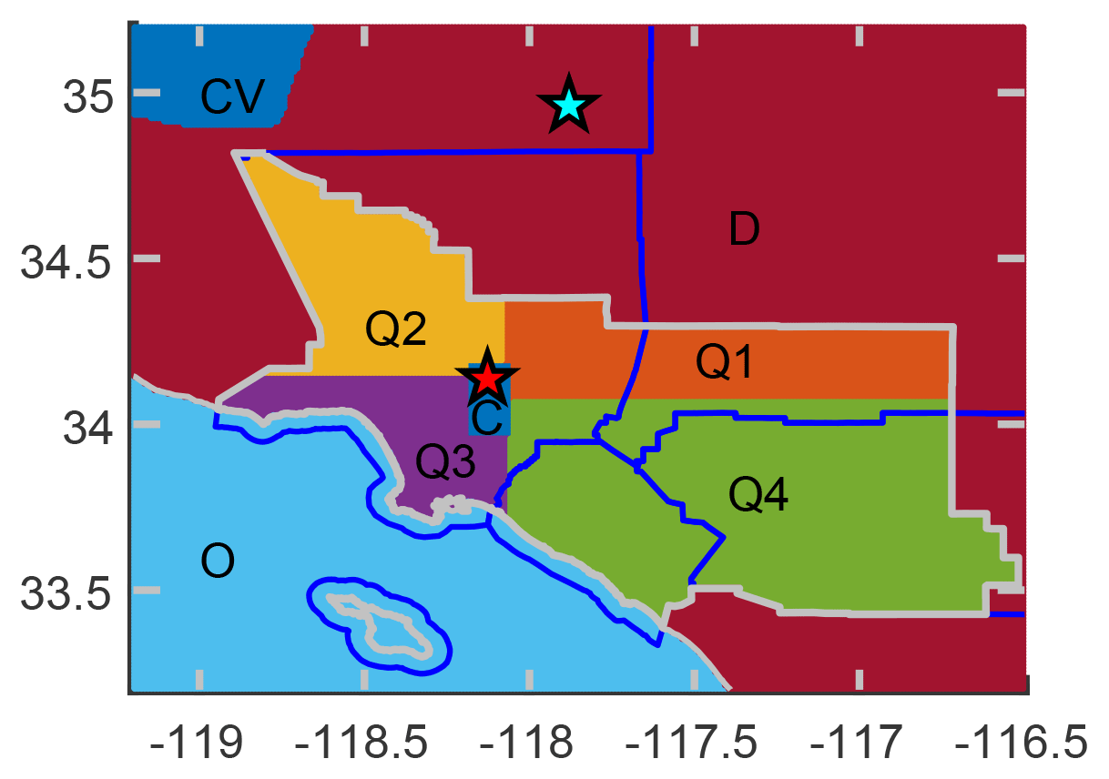
Figure E1Extent of the eight spatial subregions. C: center; Q1–Q4: SoCAB quadrants; O: ocean; CV: Central Valley, D: all other areas, mostly the Mojave Desert to the northeast.
E1 Forward model
The generalized forward model can be written as
where ϵ is an error term. We test two similar forward models for the Bayesian inversions. The first is chosen to reduce the number of elements in the state vector. This choice was made based on having only two measurement locations. This model has 40 state vector scaling factors λ in seven different classes corresponding to year (6), month (12), weekday–weekend (2), time of day (6), vertical level (5), spatial bin (8), and overall (1). Time-of-day bins cover 4 h each with local ending times at 03:00, 07:00, 11:00, 15:00, 19:00, and 23:00. Aggregated vertical bins are each about 3.5 % of the atmosphere, split at 300, 612, 936, 1272, and 3200 m a.g.l. These are designed to help diagnose transport or footprint extent errors, and the upper two levels are weighted less when estimating the total SoCAB flux. Spatial bins (Fig. E1) were chosen with one over the ocean, one over Central Valley, one for the rest of the area outside the SoCAB, and five inside the SoCAB. Each SoCAB area has approximately the same influence on observations at the Caltech (abbreviated CIT) site based on residence times. This model is
Here, is the model amount determined by multiplying the residence time t by the a priori surface flux s and summing over all times and grid boxes in the bin. We use j here as shorthand for the subscript “yr, mth, dow, tod, vbin, sbin”.
We also use a similar linear model of the form
In this form there are up to nearly 35 000 original elements in our state vector as opposed to the 40 elements in Eq. (E2). Most of the original elements are not ever sampled (e.g., during 2012 and 2017) and not used when reporting our total fluxes. We remove elements that are not linearly independent, which reduces the actual number used to fewer than (about one-eighth) the number of observations. We select the most important elements from matrix R found by performing a QR decomposition on the K matrix. Changing the cutoff (and Sa) affects the sensitivity to the prior (Sect. 3).
E2 Solutions
For the linear forward model (Eq. E3), the retrieved state vector () can be found in a single step,
xa denotes the a priori state vector. Sa is the a priori covariance matrix for the state vector (denoted B in some texts). K is the m×n Jacobian matrix (denoted H in some texts). Sϵ is the m×m measurement error covariance matrix (denoted R in some texts), which includes errors from both the observations and the forward model. Sϵ is often treated as a diagonal matrix, with values along the diagonal.
For a nonlinear forward model (e.g., Eq. E2), the inverse solution can be found using an iterative Levenberg–Marquardt method. This is described in more detail by Rodgers (2000). The iterative solution is
The symbol γ is a factor chosen at each iteration to minimize the cost function based on how χ2 changes, and i+1 denotes the current iteration.
E3 A priori values
We define values for xa, Sϵ, and Sa. First, our state vector is composed of scaling factors and all elements in xa are unity for CO and CH4. Because ODIAC2016 emissions for the SoCAB are low compared to other inventories, we multiply by 1.25 for CO2. Sϵ is a diagonal matrix. Along diagonal elements are the errors from the observations plus the errors from the transport model. Observation errors are determined from Eq. (D1). We assume transport errors are constant and equal to the overall median observation error.
For simplicity, Sa is chosen as a single scalar value for the linear model (Eq. E3). We tune two parameters, namely Sa, and the threshold for determining linear independence in the QR decomposition. This is a trade-off between maximizing the degrees of freedom and r, while avoiding unstable conditions, and minimizing χ2. We scan over a variety of Sa and threshold values. We use interannual variability and dependence on the prior as noted by a sensitivity test (Fig. 7) to judge the quality. Generally as we increase the threshold fewer elements are allowed in the state vector, the dependence on the prior decreases, and the interannual range increases. As Sa increases, so does the interannual range, and the dependence on the prior decreases. We select values that keep the interannual variability under about 25 % and minimize dependence on the prior. We repeat this procedure for the three gases retrieved by TCCON and for OCO-2 observations. Sa is tuned to 0.01 for CO2, 0.007 for CH4, 0.0007 for CO, and 0.04 for CO2 using OCO-2 observations. For the 40-factor inversion, Sa is a matrix and diagonal values are the same as the linear inversion. Off-diagonal values between adjacent elements (e.g., years, months) are one-third of those along the diagonal, which is a somewhat arbitrary choice based on our a priori guess of how strongly adjacent elements are related.
JKH, JuL, and POW were involved in the overall conceptualization, investigation, and methodology development. JKH carried out the formal analysis and visualization and wrote the original draft. POW secured funding and computational resources and provided supervision. TO and SM developed the ODIAC FF inventory and provided instructions on its use. KG and JiL developed the Hestia-LA FF inventory and provided instructions on its use. CMR, LTI, JRP, PWH, DW, and POW provided TCCON data, which involved funding acquisition, site management, data processing, and QA/QC. JKH, JuL, TO, LTI, DW, and POW were involved in revising the paper.
The authors declare that they have no conflict of interest.
The authors wish to acknowledge providers of data. OCO-2 lite files were produced by the OCO-2 project at the Jet Propulsion Laboratory, California Institute of Technology. Resources supporting OCO-2 retrievals were provided by the NASA High-End Computing (HEC) Program through the NASA Advanced Supercomputing (NAS) Division at Ames Research Center. Nightlight products were obtained from the Earth Observation Group, NOAA National Geophysical Data Center and are based on Suomi NPP satellite observations. The 0.1∘ methane inventory was produced by Harvard University in collaboration with the EPA. The authors gratefully acknowledge the NOAA Air Resources Laboratory (ARL) for the provision of the HYSPLIT transport model (http://www.ready.noaa.gov, last access: 12 November 2018) as well as the gridded archived meteorological data used in this publication.
We thank Ron Cohen, Nick Parazoo, Anna Karion, and Taylor Jones for helpful discussions. We thank Nasrin Pak for discussions on landfills.
This work was financially supported by NASA's OCO-2 project (grant
no. NNN12AA01C) and NASA's carbon cycle and ecosystems research program
(grant no. NNX14AI60G and NNX17AE15G). Tomohiro Oda is supported by the NASA
Carbon Cycle Science program (grant no. NNX14AM76G). The Hestia data product
was made possible through support from Purdue University Showalter Trust, the
National Aeronautics and Space Administration grant 1491755, and the National
Institute of Standards and Technology grants 70NANB14H321 and 70NANB16H264.
The authors thank the referees for their comments.
Edited by: Robert McLaren
Reviewed by:two
anonymous referees
Andres, R. J., Boden, T. A., and Higdon, D. M.: Gridded uncertainty in fossil fuel carbon dioxide emission maps, a CDIAC example, Atmos. Chem. Phys., 16, 14979–14995, https://doi.org/10.5194/acp-16-14979-2016, 2016. a
Angevine, W. M., Eddington, L., Durkee, K., Fairall, C., Bianco, L., and Brioude, J.: Meteorological Model Evaluation for CalNex 2010, Mon. Weather Rev., 140, 3885–3906, https://doi.org/10.1175/MWR-D-12-00042.1, 2012. a
Asefi-Najafabady, S., Rayner, P. J., Gurney, K. R., McRobert, A., Song, Y., Coltin, K., Huang, J., Elvidge, C., and Baugh, K.: A multiyear, global gridded fossil fuel CO2 emission data product: Evaluation and analysis of results, J. Geophys. Res.-Atmos., 119, 213–10, https://doi.org/10.1002/2013JD021296, 2014. a
Benjamin, S. G., Weygandt, S. S., Brown, J. M., Hu, M., Alexander, C., Smirnova, T. G., Olson, J. B., James, E., Dowell, D. C., Grell, G. A., Lin, H., Peckham, S. E., Smith, T. L., Moninger, W. R., Kenyon, J., and Manikin, G. S.: A North American Hourly Assimilation and Model Forecast Cycle: The Rapid Refresh, Mon. Weather Rev., 144, 1669–1694, https://doi.org/10.1175/MWR-D-15-0242.1, 2016. a
Brioude, J., Angevine, W. M., Ahmadov, R., Kim, S. W., Evan, S., McKeen, S. A., Hsie, E. Y., Frost, G. J., Neuman, J. A., Pollack, I. B., Peischl, J., Ryerson, T. B., Holloway, J., Brown, S. S., Nowak, J. B., Roberts, J. M., Wofsy, S. C., Santoni, G. W., Oda, T., and Trainer, M.: Top-down estimate of surface flux in the Los Angeles Basin using a mesoscale inverse modeling technique: Assessing anthropogenic emissions of CO, NOx and CO2 and their impacts, Atmos. Chem. Phys., 13, 3661–3677, https://doi.org/10.5194/acp-13-3661-2013, 2013. a, b, c, d, e, f, g, h
Carranza, V., Rafiq, T., Frausto-Vicencio, I., Hopkins, F. M., Verhulst, K. R., Rao, P., Duren, R. M., and Miller, C. E.: Vista-LA: Mapping methane-emitting infrastructure in the Los Angeles megacity, Earth Syst. Sci. Data, 10, 653–676, https://doi.org/10.5194/essd-10-653-2018, 2018. a
Chen, J., Viatte, C., Hedelius, J. K., Jones, T., Franklin, J. E., Parker, H., Gottlieb, E. W., Wennberg, P. O., Dubey, M. K., and Wofsy, S. C.: Differential column measurements using compact solar-tracking spectrometers, Atmos. Chem. Phys., 16, 8479–8498, https://doi.org/10.5194/acp-16-8479-2016, 2016. a
Coniglio, M. C., Correia, J., Marsh, P. T., and Kong, F.: Verification of Convection-Allowing WRF Model Forecasts of the Planetary Boundary Layer Using Sounding Observations, Weather Forecast., 28, 842–862, https://doi.org/10.1175/WAF-D-12-00103.1, 2013. a, b
Conley, S., Franco, G., Faloona, I., Blake, D. R., Peischl, J., and Ryerson, T. B.: Methane emissions from the 2015 Aliso Canyon blowout in Los Angeles, CA, Science, 351, 1317–1320, https://doi.org/10.1126/science.aaf2348, 2016. a, b
Cui, Y. Y., Brioude, J., McKeen, S. A., Angevine, W. M., Kim, S.-W., Frost, G. J., Ahmadov, R., Peischl, J., Bousserez, N., Liu, Z., Ryerson, T. B., Wofsy, S. C., Santoni, G. W., Kort, E. A., Fischer, M. L., and Trainer, M.: Top-down estimate of methane emissions in California using a mesoscale inverse modeling technique: The South Coast Air Basin, J. Geophys. Res.-Atmos., 120, 6698–6711, https://doi.org/10.1002/2014JD023002, 2015. a
Dou, Z., Ferguson, J. D., Galligan, D. T., Kelly, A. M., Finn, S. M., and Giegengack, R.: Assessing U.S. food wastage and opportunities for reduction, Global Food Secur.-Agr., 8, 19–26, https://doi.org/10.1016/j.gfs.2016.02.001, 2016. a
Duren, R. M. and Miller, C. E.: Measuring the carbon emissions of megacities, Nat. Clim. Change, 2, 560–562, https://doi.org/10.1038/nclimate1629, 2012. a, b
European Commission, Joint Research Centre (JRC)/Netherlands Environmental Assessment Agency (PBL): Emission Database for Global Atmospheric Research (EDGAR), release version 4.2, http://edgar.jrc.ec.europa.eu (last access: 12 November 2018), 2009. a, b
Efron, B. and Gong, G.: A leisurely look at the bootstrap, the jackknife, and cross-validation, Am. Stat., 37, 36–48, https://doi.org/10.1080/00031305.1983.10483087, 1983. a
Feng, S., Lauvaux, T., Newman, S., Rao, P., Ahmadov, R., Deng, A., Díaz-Isaac, L. I., Duren, R. M., Fischer, M. L., Gerbig, C., Gurney, K. R., Huang, J., Jeong, S., Li, Z., Miller, C. E., O'Keeffe, D., Patarasuk, R., Sander, S. P., Song, Y., Wong, K. W., and Yung, Y. L.: LA Megacity: a High-Resolution Land-Atmosphere Modelling System for Urban CO2 Emissions, Atmos. Chem. Phys., 16, 9019–9045, https://doi.org/10.5194/acp-2016-143, 2016. a, b
Fischer, M. L., Parazoo, N., Brophy, K., Cui, X., Jeong, S., Liu, J., Keeling, R., Taylor, T. E., Gurney, K., Oda, T., and Graven, H.: Simulating estimation of California fossil fuel and biosphere carbon dioxide exchanges combining in situ tower and satellite column observations, J. Geophys. Res.-Atmos., 122, 3653–3671, https://doi.org/10.1002/2016JD025617, 2017. a, b, c
Gately, C. K. and Hutyra, L. R.: Large Uncertainties in Urban-Scale Carbon Emissions, J. Geophys. Res.-Atmos., 122, 242–11, https://doi.org/10.1002/2017JD027359, 2017. a
Gatz, D. F. and Smith, L.: The standard error of a weighted mean concentration – I. Bootstrapping vs other methods, Atmos. Environ., 29, 1185–1193, https://doi.org/10.1016/1352-2310(94)00210-C, 1995. a
Gurney, K. R.: The Hestia fossil fuel CO2 emissions data product for the Los Angeles Basin, Submitted to: Earth System Science Data, 2018. a
Gurney, K. R., Razlivanow, I., Song, Y., Zhou, Y., Bedrich, B., and Abdul-massih, M.: Quantification of Fossil Fuel CO2 Emissions on the Building/Street Scale for a Large US City, Environ. Sci. Technol., 46, 12194–12202, https://doi.org/10.1021/es3011282, 2012. a
Hakkarainen, J., Ialongo, I., and Tamminen, J.: Direct space-based observations of anthropogenic CO2 emission areas from OCO-2, Geophys. Res. Lett., 43, 400–411, https://doi.org/10.1002/2016GL070885, 2016. a
Hedelius, J. K., Feng, S., Roehl, C. M., Wunch, D., Hillyard, P. W., Podolske, J. R., Iraci, L. T., Patarasuk, R., Rao, P., O'Keeffe, D., Gurney, K. R., Lauvaux, T., and Wennberg, P. O.: Emissions and topographic effects on column CO2 (XCO2) variations, with a focus on the Southern California Megacity, J. Geophys. Res.-Atmos., 122, 7200–7215, https://doi.org/10.1002/2017JD026455, 2017a. a, b, c, d, e, f, g
Hedelius, J. K., Parker, H., Wunch, D., Roehl, C. M., Viatte, C., Newman, S., Toon, G. C., Podolske, J. R., Hillyard, P. W., Iraci, L. T., Dubey, M. K., and Wennberg, P. O.: Intercomparability of XCO2 and XCH4 from the United States TCCON sites, Atmos. Meas. Tech., 10, 1481–1493, https://doi.org/10.5194/amt-10-1481-2017, 2017b. a
Hsu, Y.-K., VanCuren, T., Park, S., Jakober, C., Herner, J., FitzGibbon, M., Blake, D. R., and Parrish, D. D.: Methane emissions inventory verification in southern California, Atmos. Environ., 44, 1–7, https://doi.org/10.1016/j.atmosenv.2009.10.002, 2010. a, b
Iraci, L., Podolske, J., Hillyard, P., Roehl, C., Wennberg, P. O., Blavier, J.-F., Landeros, J., Allen, N., Wunch, D., Zavaleta, J., Quigley, E., Osterman, G., Albertson, R., Dunwoody, K., and Boyden., H.: TCCON data from Armstrong Flight Research Center, Edwards, CA, USA, Release GGG2014R1, https://doi.org/10.14291/tccon.ggg2014.edwards01.R1/1255068, 2014. a
Janardanan, R., Maksyutov, S., Oda, T., Saito, M., Kaiser, J. W., Ganshin, A., Stohl, A., Matsunaga, T., Yoshida, Y., and Yokota, T.: Comparing GOSAT observations of localized CO2 enhancements by large emitters with inventory-based estimates, Geophys. Res. Lett., 43, 3486–3493, https://doi.org/10.1002/2016GL067843, 2016. a, b, c, d
Kleiman, G. and Prinn, R. G.: Measurement and deduction of emissions of trichloroethene, tetrachloroethene, and trichloromethane (chloroform) in the northeastern United States and southeastern Canada, J. Geophys. Res.-Atmos., 105, 28875–28893, https://doi.org/10.1029/2000JD900513, 2000. a, b, c
Kopacz, M., Jacob, D. J., Henze, D. K., Heald, C. L., Streets, D. G., and Zhang, Q.: Comparison of adjoint and analytical Bayesian inversion methods for constraining Asian sources of carbon monoxide using satellite (MOPITT) measurements of CO columns, J. Geophys. Res.-Atmos., 114, 1–10, https://doi.org/10.1029/2007JD009264, 2009. a
Kort, E. A., Frankenberg, C., Miller, C. E., and Oda, T.: Space-based observations of megacity carbon dioxide, Geophys. Res. Lett., 39, 1–5, https://doi.org/10.1029/2012GL052738, 2012. a, b, c, d, e, f
Kulawik, S., Wunch, D., O'Dell, C., Frankenberg, C., Reuter, M., Oda, T., Chevallier, F., Sherlock, V., Buchwitz, M., Osterman, G., Miller, C. E., Wennberg, P. O., Griffith, D., Morino, I., Dubey, M. K., Deutscher, N. M., Notholt, J., Hase, F., Warneke, T., Sussmann, R., Robinson, J., Strong, K., Schneider, M., De Mazière, M., Shiomi, K., Feist, D. G., Iraci, L. T., and Wolf, J.: Consistent evaluation of ACOS-GOSAT, BESD-SCIAMACHY, CarbonTracker, and MACC through comparisons to TCCON, Atmos. Meas. Tech., 9, 683–709, https://doi.org/10.5194/amt-9-683-2016, 2016. a
Lauvaux, T., Miles, N. L., Deng, A., Richardson, S. J., Cambaliza, M. O., Davis, K. J., Gaudet, B., Gurney, K. R., Huang, J., O'Keefe, D., Song, Y., Karion, A., Oda, T., Patarasuk, R., Razlivanov, I., Sarmiento, D., Shepson, P., Sweeney, C., Turnbull, J., and Wu, K.: High-resolution atmospheric inversion of urban CO2 emissions during the dormant season of the Indianapolis Flux Experiment (INFLUX), J. Geophys. Res.-Atmos., 121, 5213–5236, https://doi.org/10.1002/2015JD024473, 2016. a, b, c, d
Liu, J., Bowman, K. W., Schimel, D. S., Parazoo, N. C., Jiang, Z., Lee, M., Bloom, A. A., Wunch, D., Frankenberg, C., Sun, Y., O'Dell, C. W., Gurney, K. R., Menemenlis, D., Gierach, M., Crisp, D., and Eldering, A.: Contrasting carbon cycle responses of the tropical continents to the 2015–2016 El Niño, Science, 358, eaam5690, https://doi.org/10.1126/science.aam5690, 2017. a
Maasakkers, J. D., Jacob, D. J., Sulprizio, M. P., Turner, A. J., Weitz, M., Wirth, T., Hight, C., DeFigueiredo, M., Desai, M., Schmeltz, R., Hockstad, L., Bloom, A. A., Bowman, K. W., Jeong, S., and Fischer, M. L.: Gridded National Inventory of U.S. Methane Emissions, Environ. Sci. Technol., 50, 13123–13133, https://doi.org/10.1021/acs.est.6b02878, 2016. a, b, c
Mitchell, L. E., Lin, J. C., Bowling, D. R., Pataki, D. E., Strong, C., Schauer, A. J., Bares, R., Bush, S. E., Stephens, B. B., Mendoza, D., Mallia, D., Holland, L., Gurney, K. R., and Ehleringer, J. R.: Long-term urban carbon dioxide observations reveal spatial and temporal dynamics related to urban characteristics and growth, P. Natl. Acad. Sci. USA, 115, 2912–2917, https://doi.org/10.1073/pnas.1702393115, 2018. a
Nassar, R., Napier-Linton, L., Gurney, K. R., Andres, R. J., Oda, T., Vogel, F. R., and Deng, F.: Improving the temporal and spatial distribution of CO2 emissions from global fossil fuel emission data sets, J. Geophys. Res.-Atmos., 118, 917–933, https://doi.org/10.1029/2012JD018196, 2013. a, b
Newman, S., Xu, X., Gurney, K. R., Hsu, Y. K., Li, K. F., Jiang, X., Keeling, R., Feng, S., O'Keefe, D., Patarasuk, R., Wong, K. W., Rao, P., Fischer, M. L., and Yung, Y. L.: Toward consistency between trends in bottom-up CO2 emissions and top-down atmospheric measurements in the Los Angeles megacity, Atmos. Chem. Phys., 16, 3843–3863, https://doi.org/10.5194/acp-16-3843-2016, 2016. a, b, c, d
OCO-2 Science Team, Gunson, M., and Eldering, A.: OCO-2 Level 2 bias-corrected XCO2 and other select fields from the full-physics retrieval aggregated as daily files, Retrospective processing V8r, https://doi.org/10.5067/XR7ZWYSKP7D0, 2017. a
Oda, T. and Maksyutov, S.: A very high-resolution (1 km × 1 km) global fossil fuel CO2 emission inventory derived using a point source database and satellite observations of nighttime lights, Atmos. Chem. Phys., 11, 543–556, https://doi.org/10.5194/acp-11-543-2011, 2011. a
Oda, T. and Maksyutov, S.: ODIAC Fossil Fuel CO2 Emissions Dataset (Version ODIAC2016), Center for Global Environmental Research, National Institute for Environmental Studies, https://doi.org/10.17595/20170411.001, 2015. a
Oda, T., Lauvaux, T., Lu, D., Rao, P., Miles, N. L., Richardson, S. J., and Gurney, K. R.: On the impact of granularity of space-based urban CO2 emissions in urban atmospheric inversions: A case study for Indianapolis, IN, Elem. Sci. Anth., 5, 12 pp., https://doi.org/10.1525/elementa.146, 2017. a, b
Oda, T., Maksyutov, S., and Andres, R. J.: The Open-source Data Inventory for Anthropogenic CO2, version 2016 (ODIAC2016): a global monthly fossil fuel CO2 gridded emissions data product for tracer transport simulations, Earth Syst. Sci. Data, 10, 87–107, https://doi.org/10.5194/essd-10-87-2018, 2018. a, b
O'Dell, C. W., Eldering, A., Wennberg, P. O., Crisp, D., Gunson, M. R., Fisher, B., Frankenberg, C., Kiel, M., Lindqvist, H., Mandrake, L., Merrelli, A., Natraj, V., Nelson, R. R., Osterman, G. B., Payne, V. H., Taylor, T. R., Wunch, D., Drouin, B. J., Oyafuso, F., Chang, A., McDuffie, J., Smyth, M., Baker, D. F., Basu, S., Chevallier, F., Crowell, S. M. R., Feng, L., Palmer, P. I., Dubey, M., García, O. E., Griffith, D. W. T., Hase, F., Iraci, L. T., Kivi, R., Morino, I., Notholt, J., Ohyama, H., Petri, C., Roehl, C. M., Sha, M. K., Strong, K., Sussmann, R., Te, Y., Uchino, O., and Velazco, V. A.: Improved Retrievals of Carbon Dioxide from the Orbiting Carbon Observatory-2 with the version 8 ACOS algorithm, Atmos. Meas. Tech. Discuss., https://doi.org/10.5194/amt-2018-257, in review, 2018. a
Park, C., Gerbig, C., Newman, S., Ahmadov, R., Feng, S., Gurney, K. R., Carmichael, G. R., Park, S. Y., Lee, H. W., Goulden, M., Stutz, J., Peischl, J., and Ryerson, T.: CO2 transport, variability, and budget over the Southern California Air Basin using the high-resolution WRF-VPRM model during the CalNex 2010 campaign, J. Appl. Meteorol. Climatol., 57, 1337–1352, https://doi.org/10.1175/JAMC-D-17-0358.1, 2018. a
Peischl, J., Ryerson, T. B., Brioude, J., Aikin, K. C., Andrews, A. E., Atlas, E., Blake, D., Daube, B. C., de Gouw, J. A., Dlugokencky, E., Frost, G. J., Gentner, D. R., Gilman, J. B., Goldstein, A. H., Harley, R. A., Holloway, J. S., Kofler, J., Kuster, W. C., Lang, P. M., Novelli, P. C., Santoni, G. W., Trainer, M., Wofsy, S. C., and Parrish, D. D.: Quantifying sources of methane using light alkanes in the Los Angeles basin, California, J. Geophys. Res.-Atmos., 118, 4974–4990, https://doi.org/10.1002/jgrd.50413, 2013. a, b, c
Pollack, I. B., Ryerson, T. B., Trainer, M., Parrish, D. D., Andrews, A. E., Atlas, E. L., Blake, D. R., Brown, S. S., Commane, R., Daube, B. C., de Gouw, J. A., Dubé, W. P., Flynn, J., Frost, G. J., Gilman, J. B., Grossberg, N., Holloway, J. S., Kofler, J., Kort, E. A., Kuster, W. C., Lang, P. M., Lefer, B., Lueb, R. A., Neuman, J. A., Nowak, J. B., Novelli, P. C., Peischl, J., Perring, A. E., Roberts, J. M., Santoni, G., Schwarz, J. P., Spackman, J. R., Wagner, N. L., Warneke, C., Washenfelder, R. A., Wofsy, S. C., and Xiang, B.: Airborne and ground-based observations of a weekend effect in ozone, precursors, and oxidation products in the California South Coast Air Basin, J. Geophys. Res.-Atmos., 117, D00V05, https://doi.org/10.1029/2011JD016772, 2012. a, b, c
Prairie, Y. T. and Duarte, C. M.: Direct and indirect metabolic CO2 release by humanity, Biogeosciences, 4, 215–217, https://doi.org/10.5194/bg-4-215-2007, 2007. a, b
Rodgers, C. D.: Inverse Methods for Atmospheric Sounding - Theory and Practice, vol. 2 of Series on Atmospheric Oceanic and Planetary Physics, World Scientific Publishing Co. Pte. Ltd., https://doi.org/10.1142/9789812813718, 2000. a, b, c, d, e
RTI: Draft – Greenhouse Gas Emissions Estimation Methodologies for Biogenic Emissions from Selected Source Categories: Solid Waste Disposal Wastewater Treatment Ethanol Fermentation, Tech. rep., Research Triangle Institute (RTI), Research Triangle Park, NC, USA, https://www3.epa.gov/ttn/chief/efpac/ghg/GHG_Biogenic_Report_draft_Dec1410.pdf (last access: 12 November 2018), 2010. a
Sargent, M., Barrera, Y., Nehrkorn, T., Hutyra, L. R., Gately, C. K., Jones, T., McKain, K., Sweeney, C., Hegarty, J., Hardiman, B., and Wofsy, S. C.: Anthropogenic and biogenic CO2 fluxes in the Boston urban region, P. Natl. Acad. Sci. USA, 115, 7491–7496, https://doi.org/10.1073/pnas.1803715115, 2018. a, b
Schwandner, F. M., Gunson, M. R., Miller, C. E., Carn, S. A., Eldering, A., Krings, T., Verhulst, K. R., Schimel, D. S., Nguyen, H. M., Crisp, D., O’Dell, C. W., Osterman, G. B., Iraci, L. T., and Podolske, J. R.: Spaceborne detection of localized carbon dioxide sources, Science, 358, eaam5782, https://doi.org/10.1126/science.aam5782, 2017. a, b, c, d
Seto, K. C. and Dhakal, S.: Human Settlements, Infrastructure, and Spatial Planning, Climate change 2014: Mitigation of climate change. Contribution of Working Group III to the Fifth Assessment Report of the Intergovernmental Panel on Climate Change, Chapter 12, 923–1000, https://doi.org/10.1017/CBO9781107415416.018, 2014. a
Shusterman, A. A., Teige, V. E., Turner, A. J., Newman, C., Kim, J., and Cohen, R. C.: The Berkeley Atmospheric CO2 Observation Network: Initial evaluation, Atmos. Chem. Phys., 16, 13449–13463, https://doi.org/10.5194/acp-16-13449-2016, 2016. a
Silva, S. and Arellano, A.: Characterizing Regional-Scale Combustion Using Satellite Retrievals of CO, NO2 and CO2, Remote Sens., 9, 744 (15 pp.), https://doi.org/10.3390/rs9070744, 2017. a
Silva, S. J., Arellano, A. F., and Worden, H. M.: Toward anthropogenic combustion emission constraints from space-based analysis of urban CO2 ∕ CO sensitivity, Geophys. Res. Lett., 40, 4971–4976, https://doi.org/10.1002/grl.50954, 2013. a
Small, C., Pozzi, F., and Elvidge, C. D.: Spatial analysis of global urban extent from DMSP-OLS night lights, Remote Sens. Environ., 96, 277–291, https://doi.org/10.1016/j.rse.2005.02.002, 2005. a
Stein, A. F., Draxler, R. R., Rolph, G. D., Stunder, B. J. B., Cohen, M. D., and Ngan, F.: Noaa's hysplit atmospheric transport and dispersion modeling system, B. Am. Meteorol. Soc., 96, 2059–2077, https://doi.org/10.1175/BAMS-D-14-00110.1, 2015. a
Turner, A. J., Shusterman, A. A., McDonald, B. C., Teige, V., Harley, R. A., and Cohen, R. C.: Network design for quantifying urban CO2 emissions: Assessing trade-offs between precision and network density, Atmos. Chem. Phys., 16, 13465–13475, https://doi.org/10.5194/acp-16-13465-2016, 2016. a, b, c
Verhulst, K. R., Karion, A., Kim, J., Salameh, P. K., Keeling, R. F., Newman, S., Miller, J., Sloop, C., Pongetti, T., Rao, P., Wong, C., Hopkins, F. M., Yadav, V., Weiss, R. F., Duren, R. M., and Miller, C. E.: Carbon dioxide and methane measurements from the Los Angeles Megacity Carbon Project – Part 1: Calibration, urban enhancements, and uncertainty estimates, Atmos. Chem. Phys., 17, 8313–8341, https://doi.org/10.5194/acp-17-8313-2017, 2017. a, b, c, d
Viatte, C., Lauvaux, T., Hedelius, J. K., Parker, H., Chen, J., Jones, T., Franklin, J. E., Deng, A. J., Gaudet, B., Verhulst, K., Duren, R., Wunch, D., Roehl, C., Dubey, M. K., Wofsy, S., and Wennberg, P. O.: Methane emissions from dairies in the Los Angeles Basin, Atmos. Chem. Phys., 17, 7509–7528, https://doi.org/10.5194/acp-17-7509-2017, 2017. a
Wecht, K. J., Jacob, D. J., Sulprizio, M. P., Santoni, G. W., Wofsy, S. C., Parker, R., Bösch, H., and Worden, J.: Spatially resolving methane emissions in California: constraints from the CalNex aircraft campaign and from present (GOSAT, TES) and future (TROPOMI, geostationary) satellite observations, Atmos. Chem. Phys., 14, 8173–8184, https://doi.org/10.5194/acp-14-8173-2014, 2014. a, b
Wennberg, P. O., Mui, W., Wunch, D., Kort, E. A., Blake, D. R., Atlas, E. L., Santoni, G. W., Wofsy, S. C., Diskin, G. S., Jeong, S., and Fischer, M. L.: On the sources of methane to the Los Angeles atmosphere, Environ. Sci. Technol., 46, 9282–9269, https://doi.org/10.1021/es301138y, 2012. a, b, c
Wennberg, P. O., Wunch, D., Roehl, C., Blavier, J.-F., Toon, G. C., and Allen, N.: TCCON data from California Institute of Technology, Pasadena, California, USA, Release GGG2014R1, https://doi.org/10.14291/tccon.ggg2014.pasadena01.R1/1182415, 2014. a
Wong, C. K., Pongetti, T. J., Oda, T., Rao, P., Gurney, K. R., Newman, S., Duren, R. M., Miller, C. E., Yung, Y. L., and Sander, S. P.: Monthly trends of methane emissions in Los Angeles from 2011 to 2015 inferred by CLARS-FTS observations, Atmos. Chem. Phys., 16, 13121–13130, https://doi.org/10.5194/acp-16-13121-2016, 2016. a, b, c, d
Wong, K. W., Fu, D., Pongetti, T. J., Newman, S., Kort, E. A., Duren, R., Hsu, Y. K., Miller, C. E., Yung, Y. L., and Sander, S. P.: Mapping CH4 : CO2 ratios in Los Angeles with CLARS-FTS from Mount Wilson, California, Atmos. Chem. Phys., 15, 241–252, https://doi.org/10.5194/acp-15-241-2015, 2015. a, b, c
Worden, R. J., Doran, G., Kulawik, S., Eldering, A., Crisp, D., Frankenberg, C., O'Dell, C., and Bowman, K.: Evaluation and attribution of OCO-2 XCO2 uncertainties, Atmos. Meas. Tech., 10, 2759–2771, https://doi.org/10.5194/amt-10-2759-2017, 2017. a
Wu, D., Lin, J. C., Oda, T., Ye, X., Lauvaux, T., Yang, E. G., and Kort, E. A.: A Lagrangian Approach Towards Extracting Signals of Urban CO2 Emissions from Satellite Observations of Atmospheric Column CO2 (XCO2): X-Stochastic Time-Inverted Lagrangian Transport model (“X-STILT v1.1”), Geosci. Model Dev. Discuss., https://doi.org/10.5194/gmd-2018-123, in review, 2018. a, b
Wunch, D., Wennberg, P. O., Toon, G. C., Keppel-Aleks, G., and Yavin, Y. G.: Emissions of greenhouse gases from a North American megacity, Geophys. Res. Lett., 36, L15810, https://doi.org/10.1029/2009GL039825, 2009. a, b, c, d, e, f, g, h, i, j, k, l, m
Wunch, D., Toon, G. C., Sherlock, V., Deutscher, N. M., Liu, C., Feist, D. G., and Wennberg, P. O.: The Total Carbon Column Observing Network's GGG2014 Data Version, p. 43, https://doi.org/10.14291/tccon.ggg2014.documentation.R0/1221662, 2015. a, b
Wunch, D., Toon, G. C., Hedelius, J., Vizenor, N., Roehl, C. M., Saad, K. M., Blavier, J.-F. L., Blake, D. R., and Wennberg, P. O.: Quantifying the loss of processed natural gas within California's South Coast Air Basin using long-term measurements of ethane and methane, Atmos. Chem. Phys., 16, 14091–14105, https://doi.org/10.5194/acp-16-14091-2016, 2016. a, b, c, d, e
Wunch, D., Wennberg, P. O., Osterman, G., Fisher, B., Naylor, B., Roehl, C. M., O'Dell, C., Mandrake, L., Viatte, C., Kiel, M., Griffith, D. W. T., Deutscher, N. M., Velazco, V. A., Notholt, J., Warneke, T., Petri, C., De Maziere, M., Sha, M. K., Sussmann, R., Rettinger, M., Pollard, D., Robinson, J., Morino, I., Uchino, O., Hase, F., Blumenstock, T., Feist, D. G., Arnold, S. G., Strong, K., Mendonca, J., Kivi, R., Heikkinen, P., Iraci, L., Podolske, J., Hillyard, P. W., Kawakami, S., Dubey, M. K., Parker, H. A., Sepulveda, E., Garcia, O. E., Te, Y., Jeseck, P., Gunson, M. R., Crisp, D., and Eldering, A.: Comparisons of the Orbiting Carbon Observatory-2 (OCO-2) measurements with TCCON, Atmos. Meas. Tech., 10, 2209–2238, https://doi.org/10.5194/amt-10-2209-2017, 2017. a, b
Ye, X., Lauvaux, T., Kort, E. A., Oda, T., Feng, S., Lin, J. C., Yang, E., and Wu, D.: Constraining fossil fuel CO2 emissions from urban area using OCO-2 observations of total column CO2, Atmos. Chem. Phys. Discuss., https://doi.org/10.5194/acp-2017-1022, in review, 2017. a, b, c, d, e
York, D., Evensen, N. M., Martinez, M. L., and De Basabe Delgado, J.: Unified equations for the slope, intercept, and standard errors of the best straight line, Am. J. Phys., 72, 367–375, https://doi.org/10.1119/1.1632486, 2004. a
- Abstract
- Introduction
- Data sources and methods
- Typical Xgas enhancements
- SoCAB flux estimates
- Discussion
- Conclusions
- Data availability
- Appendix A: Observation data filtering and boundary condition
- Appendix B: Dynamical model error
- Appendix C: Residence times from HYSPLIT
- Appendix D: Kalman filter
- Appendix E: Bayesian inversions
- Author contributions
- Competing interests
- Acknowledgements
- References