the Creative Commons Attribution 4.0 License.
the Creative Commons Attribution 4.0 License.
 | 15 Nov 2018
Global IWV trends and variability in atmospheric reanalyses and GPS observations
Ana C. Parracho
Olivier Bock
Sophie Bastin
This study investigates the means, variability, and trends in integrated water vapour (IWV) from two modern reanalyses (ERA-Interim and MERRA-2) from 1980 to 2016 and ground-based GPS data from 1995 to 2010. It is found that the mean distributions and inter-annual variability in IWV in the reanalyses and GPS are consistent, even in regions of strong gradients. ERA-Interim is shown to exhibit a slight moist bias in the extra-tropics and a slight dry bias in the tropics (both on the order of 0.5 to 1 kg m−2) compared to GPS. ERA-Interim is also generally drier than MERRA-2 over the ocean and within the tropics. Differences in variability and trends are pointed out at a few GPS sites. These differences can be due to representativeness errors (for sites located in coastal regions and regions of complex topography), gaps and inhomogeneities in the GPS series (due to equipment changes), or potential inhomogeneities in the reanalyses (due to changes in the observing system). Trends in IWV and surface temperature in ERA-Interim and MERRA-2 are shown to be consistent, with positive IWV trends generally correlated with surface warming, but MERRA-2 presents a more general global moistening trend compared to ERA-Interim. Inconsistent trends are found between the two reanalyses over Antarctica and most of the Southern Hemisphere, and over central and northern Africa. The uncertainty in current reanalyses remains quite high in these regions, where few in situ observations are available, and the spread between models is generally important. Inter-annual and decadal variations in IWV are also shown to be strongly linked with variations in the atmospheric circulation, especially in arid regions, such as northern Africa and Western Australia, which add uncertainty in the trend estimates, especially over the shorter period. In these regions, the Clausius–Clapeyron scaling ratio is found not to be a good humidity proxy for inter-annual variability and decadal trends.
- Article
(12409 KB) - Full-text XML
-
Supplement
(1204 KB) - BibTeX
- EndNote


Water vapour is a key component of the Earth's atmosphere and plays a key role in the planet's energy balance. It is the major greenhouse gas in the atmosphere and accounts for about 75 % of the total greenhouse effect globally (Kondratev, 1972). The total amount of water vapour is mainly controlled by temperature, closely following the Clausius–Clapeyron (C-C) equation (Schneider et al., 2010). Water vapour is thus an important part of the response of the climate system to external forcing, constituting a positive feedback in global warming (Held and Soden, 2006). However, at a regional scale, deviations from C-C law are observed and the strength of the feedback can vary, also because the radiative effect of absorption by water vapour is sensitive to the fractional change in water vapour, not to the absolute change (O'Gorman and Muller, 2010).
In addition, the short residence time of water vapour in the atmosphere makes its study in terms of variability and trends rather challenging. Sherwood et al. (2010) compared the long-term IWV trends reported in several studies using different datasets. Although there appears to be a global positive trend in the overall IWV data, which is consistent with a global warming trend, it is difficult to compare results from different studies, as they refer to different data sources, time periods, sites, and spatial coverage. Trenberth et al. (2005) found major problems in the means, variability, and trends from 1988 to 2001 for the National Centers for Environmental Prediction (NCEP) reanalyses 1 and 2, and for the 40-year European Centre for Medium-Range Weather Forecasts (ECMWF) reanalysis (ERA-40) over the oceans. The reanalyses showed reasonable results over land, where they are constrained by radiosonde observations. Only the reprocessed IWV data from the special sensor microwave imager (SSM/I) appeared to be realistic in terms of means, variability, and trends over the oceans. Their work points to two important issues. First, the reanalyses generally lack assimilation of water vapour information and suffer from model biases and, in the case of ERA40, problems in bias corrections with new satellites (namely after major volcano eruptions). Second, they highlight the need for the reprocessing of data and point to the shortcomings in reanalyses due to the changing observing system. The bias correction of new satellite radiances in the ECMWF reanalysis system has recently been improved using a variational bias-correction scheme, including the detection of instrument calibration errors and long-term drifts, as well as volcano eruptions (Dee and Uppala, 2009). Reduction of model biases and enhanced assimilation capabilities of satellite data (e.g. rain-affected radiances) have generally improved the water cycle in modern reanalyses. Reanalysis data generally agree well at representing the short-term variability (e.g. El Niño–Southern Oscillation, ENSO) but their ability for detecting climate trends is still debated (Dessler and Davis, 2010; Thorne and Vose, 2010; Trenberth et al., 2011; Robertson et al., 2014; Schröder et al., 2016). Chen and Liu (2016) compared the global variability and trend in water vapour in ERA-Interim and NCEP with GPS, radiosonde, and microwave satellite data, and found that ERA-Interim had better accuracy than NCEP.
In this study we will focus on analysing the mean distributions, inter-annual variability, and decadal trends from two recent reanalyses, ECMWF reanalysis ERA-Interim (Dee et al., 2011), referred to as ERAI, and the Second Modern-Era Retrospective analysis for Research and Applications, MERRA-2 (Gelaro et al., 2017). The IWV contents from the two reanalyses are intercompared and compared to a global, homogeneously reprocessed Global Positioning System (GPS) dataset over ocean and land. The ground-based GPS observations are independent from the reanalyses as they are not assimilated and thus constitute a valuable validation dataset (Bock et al., 2007; Mears et al., 2015). A critical assessment of the homogeneity of GPS dataset itself was made during this study as previous work detected small offsets associated to GPS equipment changes (Vey et al., 2009; Ning et al., 2016).
Furthermore, to add new insights in both the evaluation of ERA-Interim and MERRA-2 reanalyses and in the understanding of IWV trends and variability, we separate the analysis into seasons and consider trends and inter-annual variability of seasons. This analysis by seasons is rarely provided in other studies, although it helps to better identify regions with higher uncertainty and to understand the physical processes involved in different seasons (e.g. the dynamical component which transports moisture strongly differs between winter and summer). Trenberth et al. (2011) separated January and July in their analysis of the representation of water and energy budget in ERA-Interim and MERRA and showed the importance of studying the seasons separately. Compared to this study, we added the analysis of the GPS dataset and use MERRA-2, which benefits from several updates compared to MERRA.
This paper is organized as follows. Section 2 details the datasets and methods. Section 3 reports on the means and variability found in the GPS and reanalysis data for the 1995–2010 period. Section 4 analyses trends from ERA-Interim and MERRA-2 over the longer 1980–2016 period and focused on two regions of intense trends: Western Australia and northern Africa–eastern Sahel. Section 5 summarizes and concludes the paper.

Figure 1Map showing the 104 GPS stations used in this study. The stations discussed in the text and the Appendix are identified by their four-character ID.
2.1 Reanalysis data
In this study we use two modern reanalyses: the ECMWF reanalysis, ERA-Interim (Dee et al., 2011), and the NASA (National Aeronautics and Space Administration) reanalysis, MERRA-2 (Gelaro et al., 2017). ERA-Interim is the successor of ERA-40 and benefits from many improvements, especially a variational bias-correction scheme which reduces the impact of observing system changes. It is thus expected that trend estimates are more realistic. MERRA-2 is an update of MERRA which benefits from recent developments in NASA's Goddard Earth Observing System (GEOS) model suite, intended to address the impact of the changes in observing system (Gelaro et al., 2017). As a result, atmospheric water balance and variability in MERRA-2 are more realistic, though variations of IWV with temperature are weaker in the main satellite data reanalyses (namely ERA-Interim and MERRA-2) compared to microwave satellite observations over the oceans (Bosilovich et al., 2017).
Data from both reanalyses were extracted for the common 1980–2016 period, on regular latitude–longitude grids, at their highest horizontal resolution (0.75∘ × 0.75∘ for ERA-Interim and 0.625∘ longitude × 0.5∘ latitude for MERRA-2). In this work, the two-dimensional (2-D) distribution of IWV is investigated with reanalysis fields and with point observations from GPS data. Because GPS antenna heights and surface heights in the reanalyses are not perfectly matched (see the GPS coordinates and the heights for both reanalyses in the Supplement Table S1), the IWV estimates were adjusted for the height difference Δh based on an empirical formulation derived by Bock et al. (2005): , with Δh in metres. The advantage of this formulation is that it can be applied directly to the IWV data without requiring any auxiliary data. Its accuracy was checked compared to a more elaborate formulation using ERAI pressure level data (see Appendix B). The corrections were thus computed for each reanalysis separately using the monthly IWV data from the nearest grid point to every GPS station.
2.2 GPS data
We used the reprocessed tropospheric delay data from GPS stations of the International GNSS (Global Navigation Satellite System) Service (IGS) network (Fig. 1). The data was reprocessed by the NASA Jet Propulsion Laboratory (JPL) in 2010–2011 and is referred to as IGS repro1. Basic details on the processing procedure are described by Byun and Bar-Server (2009) for the operational version at the time. The reprocessed data set was produced with more recent observation models (e.g. mapping functions, absolute antenna models) and consistently reprocessed satellite orbits and clocks (IGSMAIL-6298, 2012). Inspection of file headers revealed that the processing options were not updated for a small number of stations for a period of nearly 1 year between March 2008 and March 2009. The comparison of solutions with old and new processing options (available for the year 2007) showed that this inconsistency in the processing has negligible impact at most stations, except for stations at high southern latitudes (e.g. in Antarctica). The data set covers the period from January 1995 to December 2010 for 456 stations. Among these, 120 stations have time series with only small gaps over the 15-year period. However, the geographical distribution is quite unequal between hemispheres and even within a given hemisphere, with a cluster of 20 stations in the western USA with inter-station distance smaller than 0.75∘. In order to avoid over-representation of this region, 16 out of these 20 stations have been discarded (the selection retained those with the longer time series). The final GPS IWV dataset used in this study is thus limited to the selected 104 stations.
The basic GPS tropospheric observables are the zenith tropospheric delay (ZTD) estimates, which are available at a 5 min sampling in the IGS repro1 dataset. The GPS ZTD data were screened using an adaptation of the methods described by Bock et al. (2014, 2016). First, we applied a range check on the ZTD and formal error values using fixed thresholds according to the spatial and temporal range of expected values: 1–3 m for ZTD and 0–6 mm for formal errors. Second, we applied an outlier check based on site-specific thresholds. For ZTD, values outside the median ±0.5 m were rejected and, for formal errors, values larger than 2.5 times the median were rejected. The thresholds were recomputed for every year. Using these thresholds, we detected no ZTD values outside the limits. This is because the limits were sufficiently large to accommodate for the natural variability of ZTD values (Bock et al., 2014). On the other hand, the formal error check rejected (i.e. less than 0.1 %) of the data overall. After screening, the 5 min GPS ZTD data were averaged in 1-hourly bins.
The conversion of GPS ZTD to IWV was done using the following formula: IWV = ZWD × κ (Tm), where κ (Tm) is a function of weighted mean temperature Tm, and ZWD is the zenith wet delay, obtained from ZWD = ZTD − ZHD, and ZHD is the hydrostatic zenith delay (see Wang et al., 2005 or Bock et al., 2007 for further details). In this work, the surface pressure used to compute ZHD and the temperature and humidity profiles used to compute Tm were obtained from ERA-Interim pressure level data. The profile variables are first interpolated or extrapolated to the height of the GPS stations at the four surrounding grid points and then interpolated bi-linearly to the latitude and longitude of the GPS stations. At this stage, the 1-hourly ZTD GPS data and the 6-hourly ERA-Interim data (ZHD, Tm, and IWV) were time-matched within ±1 h. Afterwards, monthly means of the 6-hourly IWV estimates are computed and those months which have less than 60 values (i.e. at least half of the expected monthly values) are rejected. Seasonal means are computed from the monthly values when at least 2 out of 3 months are available. These selection criteria ensure that the computed values are representative of the monthly and seasonal means.
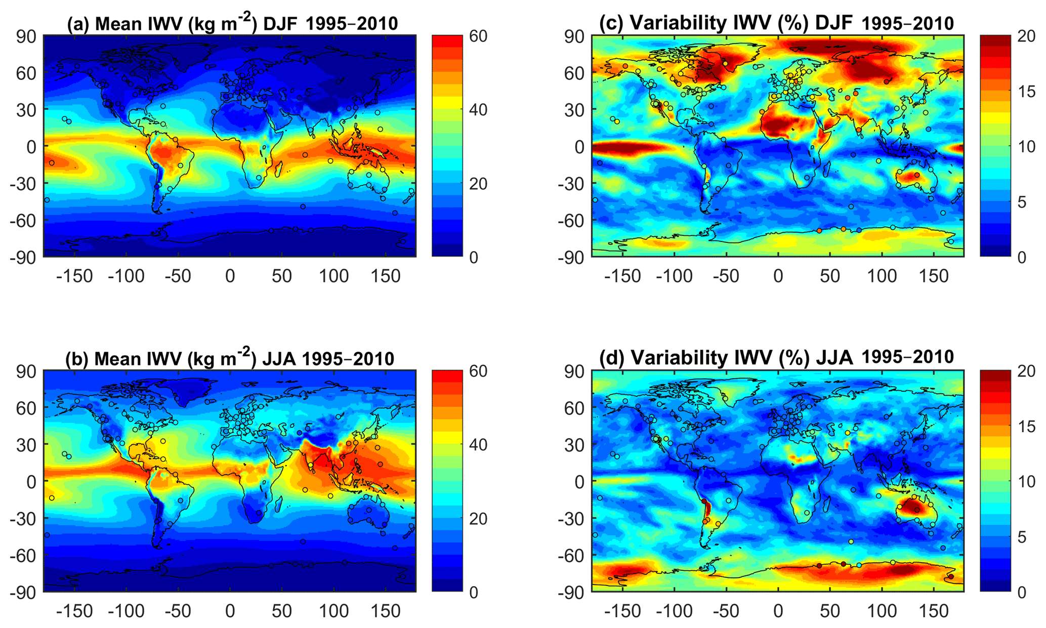
Figure 2(a) Mean IWV for DJF 1995–2010 from ERA-Interim (shading) and GPS (filled circles); (b) same as panel (a) for JJA. (c) Relative variability in percentage (%) (standard deviation of the IWV series divided by its mean) for DJF 1995–2010; (d) same as panel (c) for JJA.
In this work, inhomogeneities in the GPS IWV time series due to equipment changes were not corrected a priori, as the existing metadata may not be complete, but were rather discussed based on the intercomparison with ERA-Interim (see Appendix B). Detection and correction of inhomogeneities in the GPS ZTD and IWV data is a subject of ongoing research.
2.3 Computation of trends
The linear trends were computed using the Theil–Sen method (Theil, 1950; Sen, 1968), a non-parametric statistic that computes the median slope of all pairwise combinations of points. This method is described in more detail in the Appendix A to this paper, where it is also compared with another commonly used method for trend estimation, the least squares method.

Figure 3(a) Difference of mean IWV estimates (MERRA-2 minus ERA-Interim) for DJF 1995–2010. The global mean difference is 0.35 kg m−2 (0.94 %) and the standard deviation of the difference is 0.32 kg m−2 (1.56 %). (b) Same as panel (a) for JJA. The global mean difference is 0.56 kg m−2 (1.66 %) and the standard deviation of the difference is 0.37 kg m−2 (1.67 %). (c) Difference of relative variability estimates (MERRA-2 variability minus ERA-Interim variability) for DJF 1995–2010. The global mean difference is −0.01 % and the standard deviation of the difference is 0.26 %. (d) Same as panel (c) for JJA. The global mean difference is 0.28 % and the standard deviation of the difference is 0.42 %.
The Theil–Sen method was applied to the anomalies obtained by removing the monthly climatology from the monthly data. In the case of seasonal trends, the mean anomalies for the months of December, January, and February (DJF) and June, July, and August (JJA) were used. The statistical significance of the monthly and seasonal trends was assessed using a modified Mann–Kendall trend test (Hamed and Rao, 1998), which is suitable for autocorrelated data, at a 10 % significance level.

Figure 4(a, b) Difference of mean IWV estimates (ERA-Interim minus GPS) for DJF and JJA 1995–2010; (c, d) same as panels (a) and (b) for MERRA-2 minus GPS. The monthly data were time-matched before seasonal means were computed. (e, f) Difference of relative standard deviations of IWV estimates (ERA-Interim SD minus GPS SD.) for DJF and JJA 1995–2010; (g, h) same as panels (e) and (f) for MERRA-2 minus GPS. The monthly data were time-matched before seasonal means were computed.
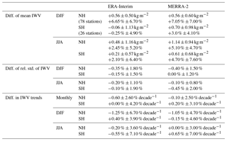
Table 1Statistics (median ± interquartile range) for the differences (ERA-Interim minus GPS and MERRA-2 minus GPS) at the 104 stations, divided by season and hemisphere, for the differences in IWV mean, relative standard deviation, and trends (ERA-Iterim).
3.1 Means and variability in IWV
The mean seasonal IWV distribution and its inter-annual variability for DJF and JJA are presented in Fig. 2. In the maps of the means (Fig. 2a, b), we can see that ERA-Interim reproduces the spatial variability well compared to GPS, including the sharper gradients in IWV, for instance, on the northern and southern flanks of the intertropical convergence zone (ITCZ) in both seasons, and in the regions of steep orography (for example, along the Andes region, in South America). Similar mean patterns are observed in MERRA-2 for both seasons, although maximum values over the ITCZ have different intensities (not shown). In order to better gauge the differences, mean difference fields between MERRA-2 and ERA-Interim are shown (Fig. 3a and b). It is observed that ERA-Interim is generally drier than MERRA-2 over the ocean and in the regions of maximum IWV, and moister in the southern part of South America, north and south of the ITCZ over Africa, and in southern (central) Asia in DJF (JJA). This result is consistent with differences between ERA-Interim and MERRA reported by Trenberth et al. (2011).
Comparing the reanalyses with GPS in Fig. 4a–d shows that both reanalyses are too moist in the Northern Hemisphere in both seasons. ERA-Interim has a dry bias at southern tropical sites in DJF and northern tropical and mid-latitude sites in JJA (especially over the USA). MERRA-2 has a moist bias overall but this is more pronounced in the Southern Hemisphere in DJF, especially over Australia, and in the Northern Hemisphere in JJA (see the increased bias over North America, northern Europe and Asia). Hemispheric and seasonal statistics can be found in Table 1 which show that in the Northern Hemisphere, the median biases of the reanalyses are very consistent in DJF (0.5–0.6 kg m−2) while in JJA the bias in MERRA-2 (1.1 kg m−2) is more than double the bias in ERA-Interim (0.48 kg m−2). In the Southern Hemisphere the main difference is for the DJF bias, which is nearly zero in ERA-Interim and 0.7 kg m−2 in MERRA-2. Similar conclusions can be drawn from the relative biases. High consistency is also seen in dispersion of the biases (inter-quartile range) between both reanalyses, with larger absolute values in the summer hemisphere and larger relative values in the winter hemisphere.
Note that in Fig. 4a–d GPS estimates at a number of sites show large biases with respect to both reanalyses. These sites are generally located in coastal regions and/or regions with complex topography, where representativeness differences can be suspected (Lorenc, 1986). We applied a statistical test to detect stations with significant differences in the mean values (with 99 % confidence level). When GPS and ERA-Interim are compared, 21 stations are detected in DJF and 18 in JJA, while with MERRA-2, 26 stations are detected in DJF and 44 in JJA. These numbers confirm in a more objective way the visual interpretation of Fig. 4. The values of all statistics can be found in the Supplement (Table S2).
For the analysis of the inter-annual variability we computed the relative standard deviation of the seasonal IWV time series (i.e. standard deviation of seasonal time series divided by its mean value). The relative variability emphasizes regions where the mean IWV contents are small (e.g. cold dry polar and/or mountainous regions and warm dry desert areas). In DJF (Fig. 2c), strong inter-annual variability (>15 %) is found in ERA-Interim for northern high-latitude regions (north-eastern Canada and eastern Greenland, the polar Arctic area, and a large part of Russia and north-eastern Asia) and for the tropical arid regions (Sahara, Arabic peninsula, central Australia). There are similar patterns of variability in MERRA-2 (not shown), with slightly higher variability in MERRA-2 over India and Antarctica. The difference fields between MERRA-2 and ERA-Interim highlight these differences (Fig. 3c). In JJA, large inter-annual variability is observed in ERA-Interim mainly over Antarctica and Australia (Fig. 2d). Locally enhanced variability is also seen over the Andes cordillera, but this is mainly due to the very low IWV values at high altitudes. MERRA-2 has similar patterns of IWV variability, with lower variability over northern Africa and north of the Andes, and higher variability over Antarctica (Fig. 3d).
In general, most of the marked regional features of inter-annual variability are confirmed by GPS observations (Fig. 2c, d). However, a few stations show different values compared to the reanalyses, but their values do not impact the variability statistics shown in Table 1 thanks to the choice of median and inter-quartile range instead of mean and standard deviation. Based on the median values, Table 1 shows that in general ERA-Interim is in slightly better agreement with GPS than MERRA-2. It also shows that both reanalyses have lower or equal variability than GPS in both hemispheres and in both seasons (negative or zero median differences of relative standard deviation in Table 1). Figure 4e–h show the spatial distribution of the differences for both reanalyses and seasons. Again, there is quite a large spatial dispersion (also revealed by the inter-quartile range in Table 1) with a number of outlying sites discussed in Appendix B.
Representativeness errors due to large spatial variations in IWV and complex topography are suspected at 20 stations. They contribute likely both to differences in the mean IWV values and in the variability. Errors in the GPS data, e.g. due to instrumental malfunctioning, measurement interferences, or changes in equipment, are also suspected at a small number of sites. Such problems can be further confirmed by comparison with IWV measurements from nearby GPS receivers or from other collocated instruments such as DORIS or VLBI (Bock et al., 2014; Ning et al., 2016). Lastly, errors in the reanalyses are suspected in data-sparse regions and regions where the performance of model physics and dynamics are poor. They are more difficult to diagnose. The differences observed between ERA-Interim and MERRA-2 might be due to a mix of differences in model physics and data assimilation.
3.2 Trends in IWV
Trends from ERA-Interim and MERRA-2 based on the time series of monthly data (hereafter referred to as monthly trends) are shown in Fig. 5. In general, there is continuity between oceanic and continental trends, suggesting a trend in air mass advections.
Both reanalyses show overall positive trends (moistening) especially marked (statistically significant) in the tropics along the ITCZ, both over the oceans and continents (northern South America, central Africa, and Indonesia in ERA-Interim) and at middle and high latitudes in the Northern Hemisphere. The moistening trends over the Arctic are significant in both reanalyses. They are interleaved with extended regions of negative (drying) trends which are statistically significant in both reanalyses over Australia, northern–central Africa, over the south-tropical eastern Pacific region, and on the oceanic border of Antarctica. The moistening–drying dipole structure in the eastern equatorial Pacific has been observed by several authors using various satellite data and reanalyses over different periods (Trenberth et al., 2005; Mieruch et al., 2014; Schröder et al., 2016; Wang et al., 2016). Trenberth et al. (2005) explained it as being due to the influence of different ENSO phases over the trends. The monthly trends computed at the GPS stations are consistent in sign and magnitude with the reanalyses where the reanalyses agree, except at a small number of GPS sites discussed in Appendix B. The trend values for ERA-Interim, MERRA-2, and GPS at all stations can be found in the Supplement (Table S3). Statistics of differences in the trend estimates between the reanalyses and GPS are given in Table 1. The median differences are small (below ±1 % decade−1) for both reanalyses and both hemispheres. The interquartile range of differences vary depending on the season and hemisphere but they are similar for both reanalyses. The monthly trends agree quite well in the Northern Hemisphere (∼2.6 % decade−1 vs. ∼4 % decade−1 in the Southern Hemisphere), while the seasonal trends have larger errors in the winter hemispheres (∼7% decade−1).

Figure 5Relative IWV trends (in % decade−1) for the 1995–2010 period from GPS (stations marked as circles), ERA-Interim (a), and MERRA-2 (b). The statistically significant trends from ERA-Interim and MERRA-2 are highlighted by stippling. Two regions discussed in Sect. 3.2 are outlined as box A (Maritime Continent) and box B (northern Africa).
Significant trend differences between MERRA-2 and ERA-Interim are seen (Fig. 5) over several parts of the globe, in particular over the Maritime Continent, northern–central Africa, central Asia, and Antarctica. In these regions the reanalyses show opposite trends. Such a discrepancy can be due to different representations of large-scale moisture transport, surface–atmosphere processes, and data assimilation in the two reanalyses.
Over the Maritime Continent (box A, in Fig. 5), ERA-Interim trends are positive while MERRA-2 trends are negative over the period from 1995 to 2010. Trenberth et al. (2005) also reported strong moistening and warming trends over the region for the 1988–2003 period using SSM/I IWV data and National Oceanic and Atmospheric Administration (NOAA) sea surface temperature (SST) data. Wang et al. (2016) confirmed the moistening but found a near-zero–slightly negative temperature trend for the 1995–2011 period (they used more recent releases of the SSM/I and NOAA data). Schröder et al. (2016) also found moistening trends in all their datasets over the 1988–2008 period, including SSM/I data and the MERRA reanalysis. Although not all studies concern the same period, they confirm the ERA-Interim results. This conclusion points to an inconsistent drying trend in MERRA-2 over the Maritime Continent. Comparison to the GPS IWV trends in Fig. 5a confirms that ERA-Interim is in better agreement with the observations than MERRA-2, though the comparison is quite difficult because there are not many GPS stations available within the domain.
Over northern Africa (box B, in Fig. 5), the drying trend in ERA-Interim reaches an extremely large value of −3.5 kg m−2 decade−1 (−17 % decade−1), which is questionable. Such a large trend would imply a significant change in the regional and global water cycle that can hardly be supported by physical arguments. Unfortunately, there are no long-term GPS data available in the region. The trends in MERRA-2 over the region are smaller and more realistic, but they also show a different spatial pattern which is questionable as well. The drying in MERRA-2 extends southward over equatorial Africa, a region where moistening is expected to follow the observed warming trends (see also Fig. 8). The difference between the reanalyses is further emphasized when comparing seasonal trends below. A major uncertainty in both reanalyses over this region is certainly due to the paucity in observations going into the assimilation. This statement is consistent with the results of Bauer (2009) and Karbou et al. (2010) who report a strong impact of humidity data from modern satellite instruments on the analysed moisture fields over the Sahara.
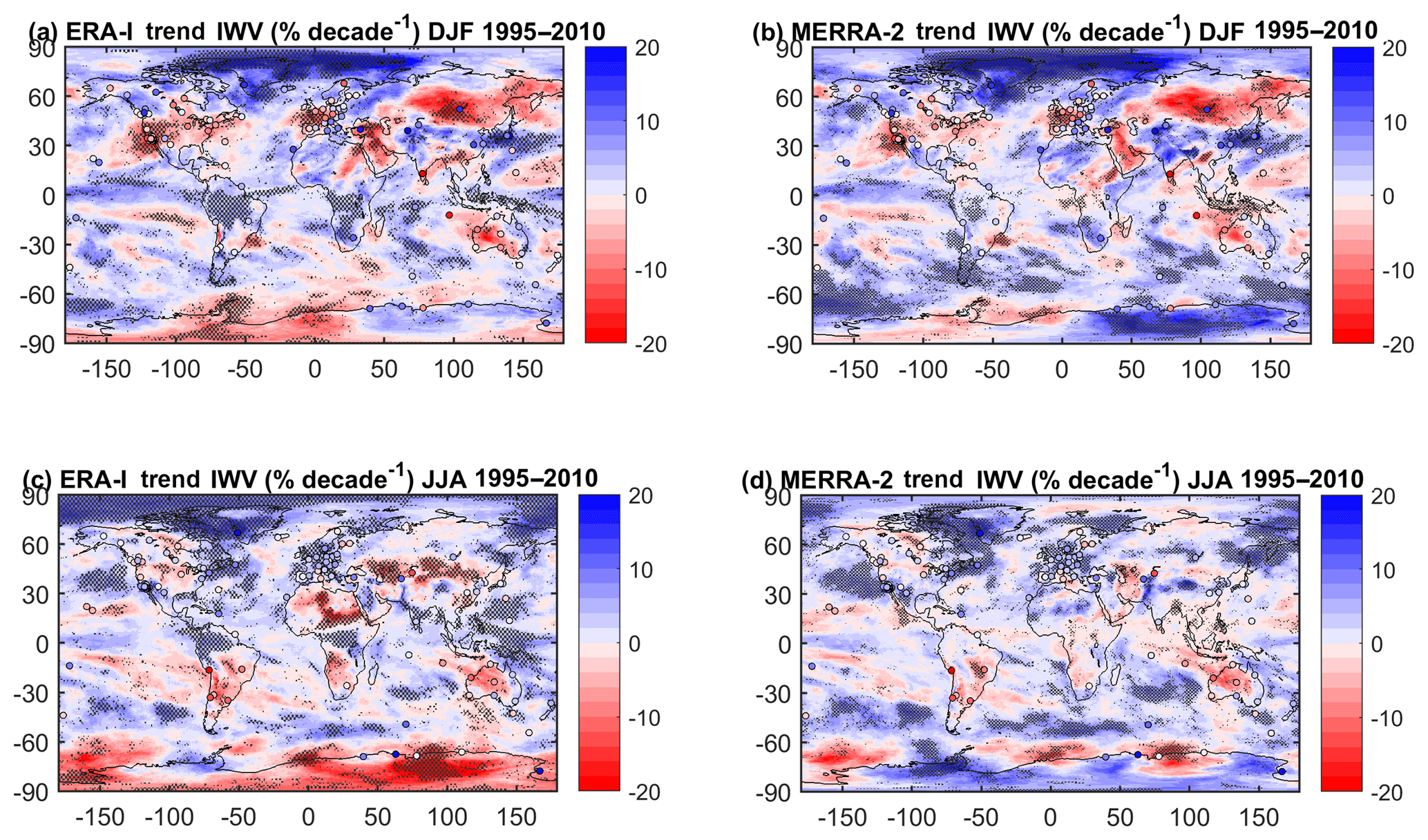
Figure 6Seasonal IWV trends for the 1995–2010 period from ERA-Interim (shading) and GPS (filled circles) for DJF (a). (b) Same as panel (a) but for MERRA-2. The statistically significant trends from the reanalyses are highlighted by stippling. (c) Same as panel (a) but for JJA. (d) Same as panel (b) but for JJA. The statistically significant trends from the reanalyses are highlighted by stippling.
Over Antarctica, the monthly trends in MERRA-2 and GPS (Fig. 5b) are significantly positive, in opposition to what is seen in ERA-Interim (Fig. 5a), where the trends are mainly negative, especially in the interior of the continent. However, one can notice that ERA-Interim shows spotted areas of positive trends in the vicinity of the GPS stations. These locally positive trends in ERA-Interim might be explained by the influence of surface and/or upper air observations collected from these sites that are assimilated in the reanalysis. Comparing ERA-Interim and MERRA-2 IWV time series in the interior of the continent reveals that the reanalyses diverge mainly before year 2000, with a positive trend in MERRA-2 between 1995 and 2000 (not shown). This divergence might be explained by a combination of differences in the observations actually assimilated and differences in the assimilation systems. Observations in the interior of the continent are most likely from satellites only. General documentation indicates that both reanalyses use the same types of satellite observations globally (Dee et al., 2011; Gelaro et al., 2017). However, the amount of assimilated data over Antarctica's ice sheet may differ between the reanalyses, which is actually not documented.
Over central and east Asia and over northern South America, ERA-Interim and MERRA-2 trends also disagree. The GPS data are in better agreement with MERRA-2 in the former region and with ERA-Interim in the latter.
Figure 6 shows the seasonal trends. A striking feature seen in both reanalyses is their relatively larger magnitude compared to the monthly trends (Fig. 5), which could be due to the fact the monthly trends use one value per month, while the seasonal trends use only one value per year. Large changes in magnitude and/or sign are also noticeable in most regions between seasons. These features emphasize that atmospheric circulation (which is largely changing between seasons) plays an important role in IWV trends.
In DFJ (Fig. 6a, b), the agreement between reanalyses is surprisingly good, given the inconsistencies pointed out from the monthly trends. The agreement of the reanalysis with GPS is also quite good, though some GPS trends are in strong contradiction (e.g. at IRKT in Siberia, KIRU in Sweden, IISC in India, and COCO east of Indonesia, which have very large magnitudes). Over Antarctica, the drying–moistening east–west dipole is consistent in both reanalyses though they are of different magnitudes. A drying–moistening dipole is also seen across Australia, consistent with the theory that precipitation over north-western Australia (the part of Australia mostly influenced by the monsoon flow in DJF) is very sensitive to the SST pattern over the western central Pacific Ocean (10∘ S–10∘ N, 150–200∘ E) (Brown et al., 2016). During the 1995–2010 period, this SST pattern has actually been warming and the atmosphere moistening, leading to a drying over north-western Australia (Wang et al., 2016).
In JJA (Fig. 6c, d), the conclusions are more contrasted. Though the reanalyses generally agree well over the oceans, except over the Maritime Continent, the trends over land are poorly consistent over most continents (Asia, Africa, South America, and Antarctica). Over these regions, the GPS trends are generally in better agreement with MERRA-2. Over northern Africa, the drying in ERA-Interim is in contradiction with the recent recovering of precipitation over western Africa (Sanogo et al., 2015). In this respect, the MERRA-2 trends are more realistic.
4.1 Global analysis
Interpretation of IWV trends of the previous section must be done cautiously as the trends have been estimated for a specific and rather short period of 15 years (from 1995–2010). They should thus not be considered as representative of a longer period and might also be impacted by decadal variability and/or large singular events such as El Niño. Trenberth et al. (2005) suggested that a longer time series may be required to obtain fully stable patterns of linear trends. In this section we will assess how consistent our trends obtained for the 1995–2010 period (when GPS data are available) are with longer-term trends computed for the full length common to ERA-Interim and MERRA-2.
Figure 7 shows the monthly trends for both reanalyses over the period 1980–2016. In both reanalyses most structures are similar to those seen for the short period (Fig. 5), although the intensities are generally weaker for the longer period (note that the colour bars are different for Figs. 5 and 7), but most of them are significant. In ERA-Interim, the main differences between periods (changes in sign of the trends) appear over the eastern tropical Pacific, Canada, the Arabic Peninsula, the region around Madagascar, Western Australia, and a small part of Antarctica. The drying trend over Australia observed for the 1995–2010 period is not observed in the long term, which suggests that there have been periods of moistening trends as part of decadal variability during the 1980–2016 period. These changes are seen in MERRA-2 as well, which gives good confidence that they are due to decadal variability in the global and regional climates. However, the main differences between reanalyses already highlighted for the short period remain (over Antarctica and the global southern oceans, northern Africa, and eastern Asia), except over the Maritime Continent where MERRA-2 now represents a moistening trend consistent with ERA-Interim and over Australia where the reanalyses now disagree.
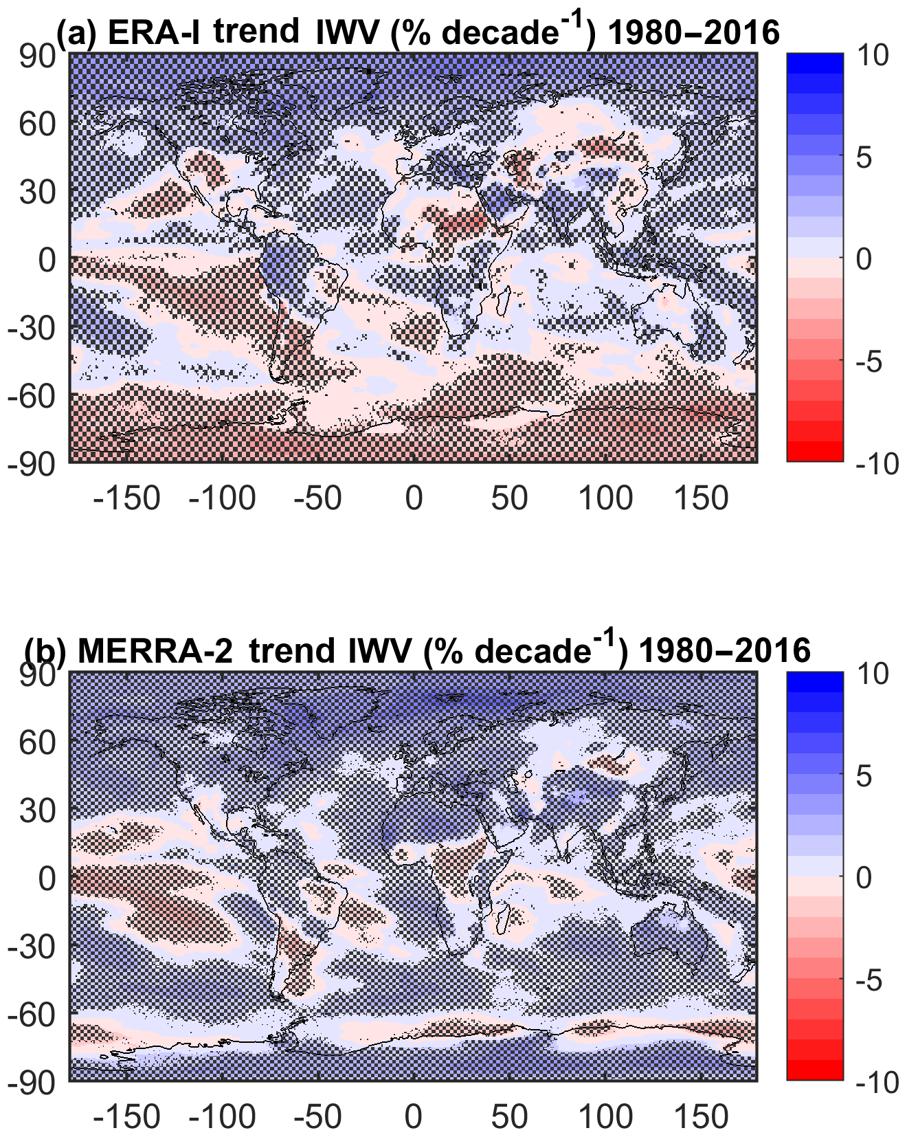
Figure 7Monthly trends in IWV for the 1980–2016 period for (a) ERA-Interim and (b) MERRA-2. The statistically significant trends are highlighted by stippling.
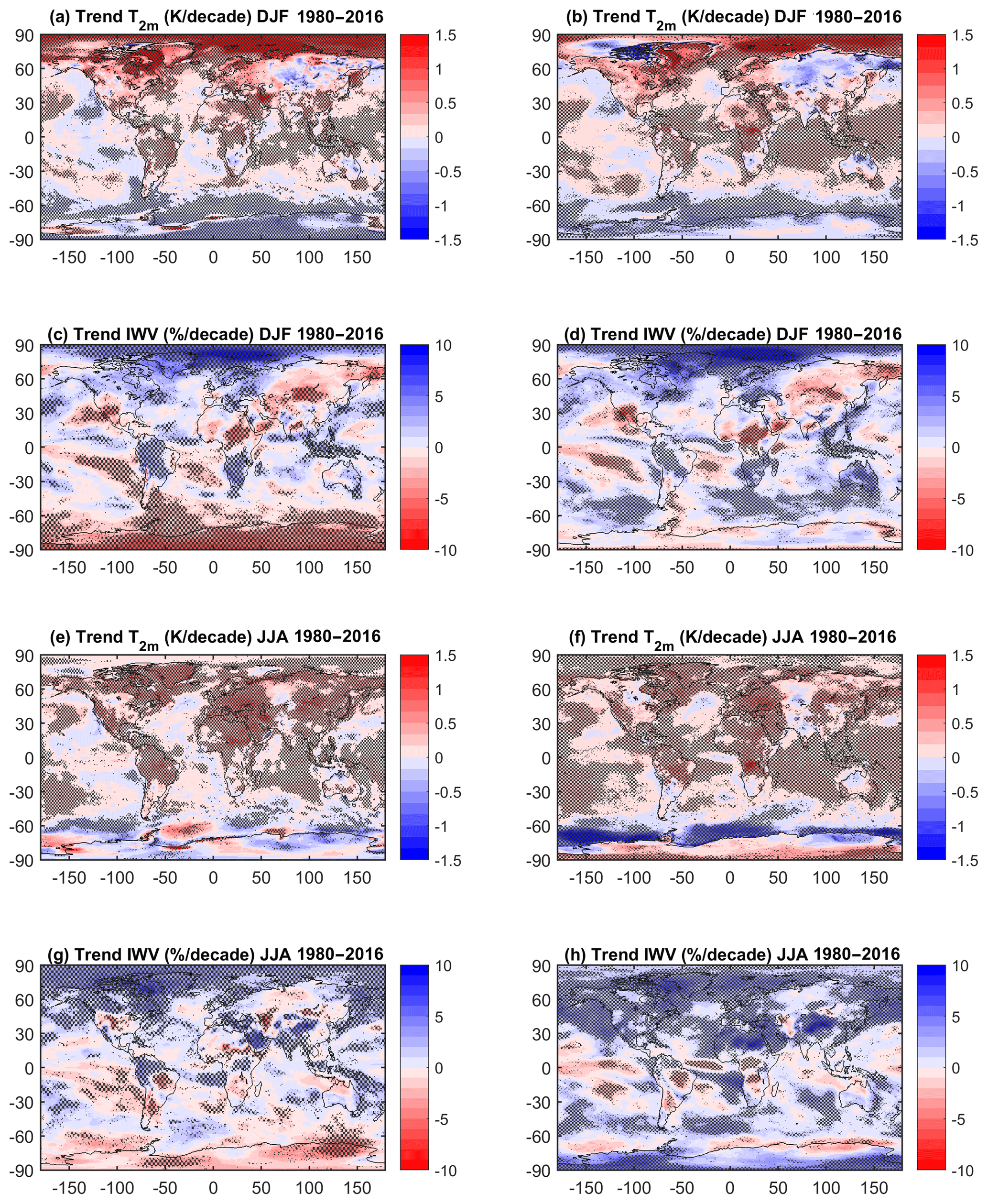
Figure 8Seasonal trends in Tm and IWV for the 1980 to 2016 period for (a, c, e, g) ERA-Interim and (b, d, f, h) MERRA-2.
Figure 8 shows the seasonal IWV trends and temperature trends. In general, it is seen that over the oceans, the temperature trends generally have the same sign as the IWV trends (but opposite colours), as expected by Clausius–Clapeyron (C-C) theory, despite some small-scale differences. Over land, most areas show an increase in temperature, except the high latitudes of the Southern Hemisphere and large parts of the Asian continent. This means that, except over Antarctica and parts of Asia, the drying observed in the aforementioned areas does not follow C-C theory. When we consider each season more closely, some areas indicate a cooling (Fig. 8a, b, e, f) consistent with a drying (Fig. 8c, d, g, h). This is observed over Antarctica (especially in ERA-Interim) and over central Asia in DJF (especially in MERRA-2). For JJA, most continental areas show a significant warming, with the exception of parts of Antarctica, a small area over northern Australia, and regions in central Asia, where a cooling is also displayed. Thus the C-C scaling ratio is not a good proxy for humidity when considering seasonal and regional variabilities and trends due to the important role of dynamics which allow the advection of dry or wet air masses (e.g. over USA, South America, eastern Sahel, and southern Africa in JJA).
Figures 7 and 8 confirm that MERRA-2 presents a more general moistening trend than ERA-Interim (as already seen over the shorter period), especially in the Southern Hemisphere in DJF (Fig. 8c, d), and in both hemispheres in JJA (Fig. 8g, h). The main differences in the trends over the oceans appear all around Antarctica, and those over continental areas are observed over Africa (where trends are positive in the north and negative in central Africa in MERRA-2 and the opposite in ERA-Interim) and USA in JJA, over Australia in DJF, and over Antarctica in both JJA and DJF. Over Africa and Antarctica, the important differences which exist between ERA-Interim and MERRA2 for both long- and short-term periods suggest that the physical processes are not well represented. These areas correspond to areas with very few observations available for data assimilation, reducing the constraint on the models. A more detailed investigation of the dynamics over Africa and Australia is presented in the next subsections.
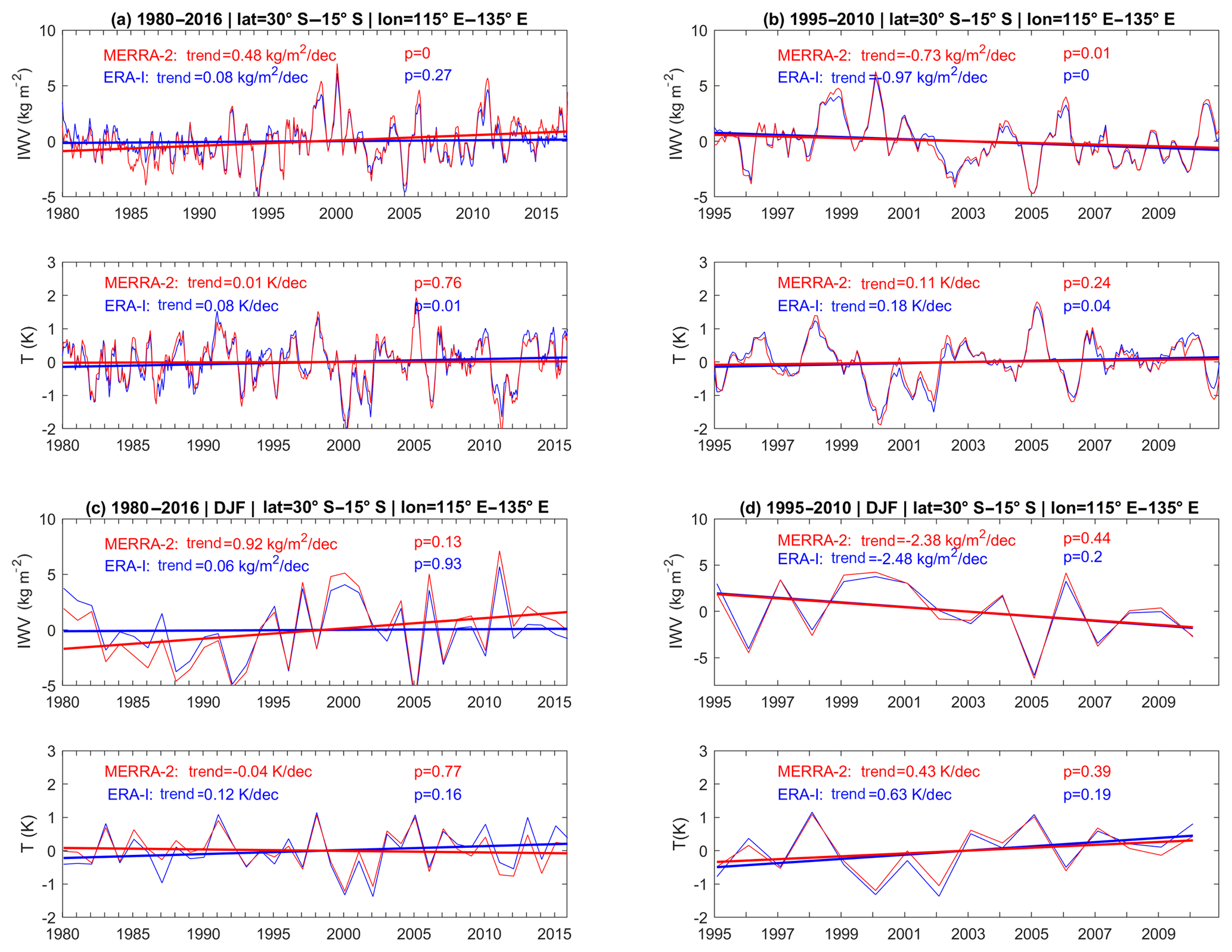
Figure 9Temperature and IWV anomaly time series for a box over Western Australia (see Fig. 14), using ERA-Interim (blue) and MERRA-2 (red) data, for (a, c) the 1980 to 2016 period, (b, d) the 1995 to 2010 period, and (a, b) the monthly time series and (c, d) the DJF season.
Other regions, such as the Indo-Pacific region, have different trends over the shorter period, but are in better agreement over the longer period. This is more obvious during JJA and can be explained by the strong variability that requires longer time series in order to obtain meaningful trends. The good agreement between reanalyses over this area is an important result in view of the fact that CMIP5 (Coupled Model Intercomparison Project Phase 5) models have large biases over this region in present-day sea surface temperature, which has direct consequences on the future projection of precipitation over Australia (Brown et al., 2016; Grose et al., 2014) and more generally over tropical and subtropical climates. Two areas are investigated in more detail in the next subsections because of the disagreement between both reanalyses over them: Australia in DJF and Africa in JJA.
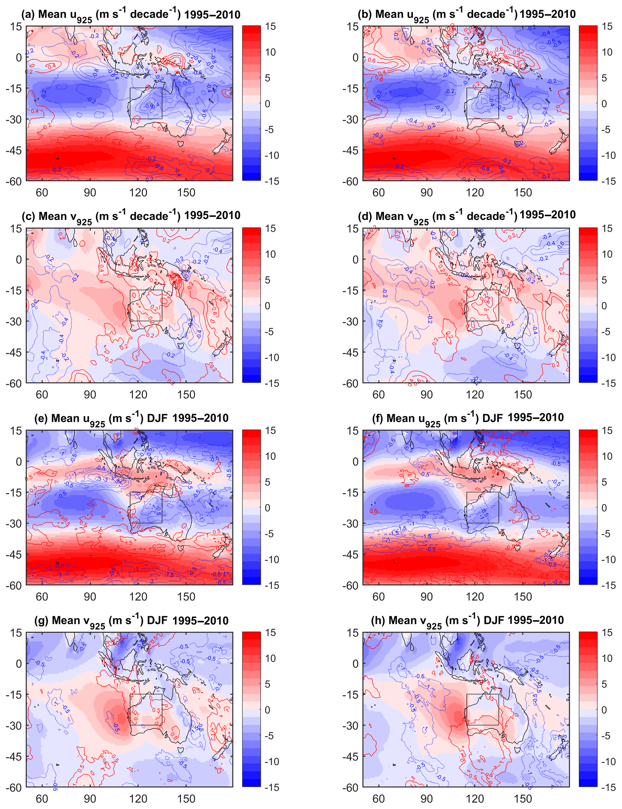
Figure 10Close-up of Western Australia showing the mean monthly and DJF fields and trends (contours) of the u and v wind components at 925 hPa (shaded). The area of focus (where IWV trends are most intense in ERA-Interim) is marked by a box.
4.2 Analysis over Western Australia
Figure 9 displays the time series of IWV and temperature anomalies for a box over Western Australia (15–30∘ S, 115–135∘ E, as shown in Fig. 10) for both the short and long periods, for both the full time series and the DJF seasons.
As can be observed in Fig. 9a, b, the moisture trend is opposite for the long (moistening) and short (drying) periods, for both reanalyses, while the temperature trend is weakly warming. However, when focusing on the DJF period (Fig. 9c, d), the differences between reanalyses are enhanced when considering the long period. ERA-Interim IWV indeed starts with higher anomalies than MERRA-2 until 1990 and ends with lower anomalies after the late 2000s, so that the resulting trend is close to zero and not significant. The different IWV trend estimates between the two periods are due to the existence of extreme cold and humid periods in both reanalyses after 1992, with a strong occurrence around the 2000s, which impact the linear trend estimate over the short period (which starts in 1995) more strongly than over the long period.
The wetter and colder summers (correlation between T and IWV being around for both reanalyses over the short period) are associated with a dynamical anomaly (not shown), with a weaker wind and a switching direction on average in the box shown in Fig. 10. As can be seen in Fig. 10 over this box, in DJF, the southern part of the box is under the influence of south-easterly wind, while the northern part of the box indicates the penetration of maritime air mass coming from the north–northwest and corresponds to the monsoon flow. The trend of the wind components in this box (indicated by the contours) show a reinforcement of the south-easterly wind to the detriment of the northern–north-western flow. The cold and wet years occurring at the beginning of the period are thus associated with a stronger monsoon flow which attenuates at the end of the period. Hence, as already mentioned by several studies (e.g. Power et al., 1998; Hendon et al., 2007) dynamics mostly explain the variability and trends of temperature and humidity over this area.
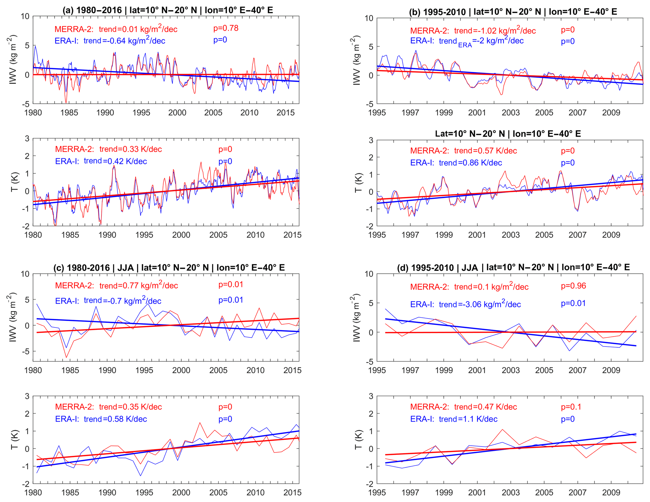
Figure 11Temperature and IWV anomalies time series for a box over the eastern Sahel (see Fig. 12), using ERA-Interim (blue) and MERRA-2 (red) data, for (a, c) the 1980 to 2016 period, (b, d) the 1995 to 2010 period, and (a, b) the monthly time series and (c, d) the JJA season.
Note that although the climatological means of zonal and meridional wind components are similar between ERA-Interim and MERRA-2, their trends over and around Australia present different patterns, especially in DJF (Fig. 10e–h), likely explaining the different IWV trends between both reanalyses.
4.3 Analysis over northern Africa–eastern Sahel
Here we focus on a box over the eastern Sahel (10–20∘ N, 10–40∘ E). The monthly trend in IWV is negative (drying) and significant in both reanalyses (except for MERRA-2 for the longer period), though it is twice as intense in ERA-Interim than in MERRA-2 (Fig. 11b). Similarly, the temperature trends are positive (warming) and significant in both reanalyses. Although the monthly anomalies show many similarities, their agreement is far from being perfect. The general strong negative IWV trend in ERA-Interim implies that IWV anomalies are higher in ERA-Interim at the beginning of the period and lower at the end of the period. However, both reanalyses present four different periods in the time IWV series: a drying trend at the very beginning (1980–1985) followed by a moistening trend until 1995, then followed by a new drying period lasting until around 2008 when the trend seems to stop (Fig. 11a, b).
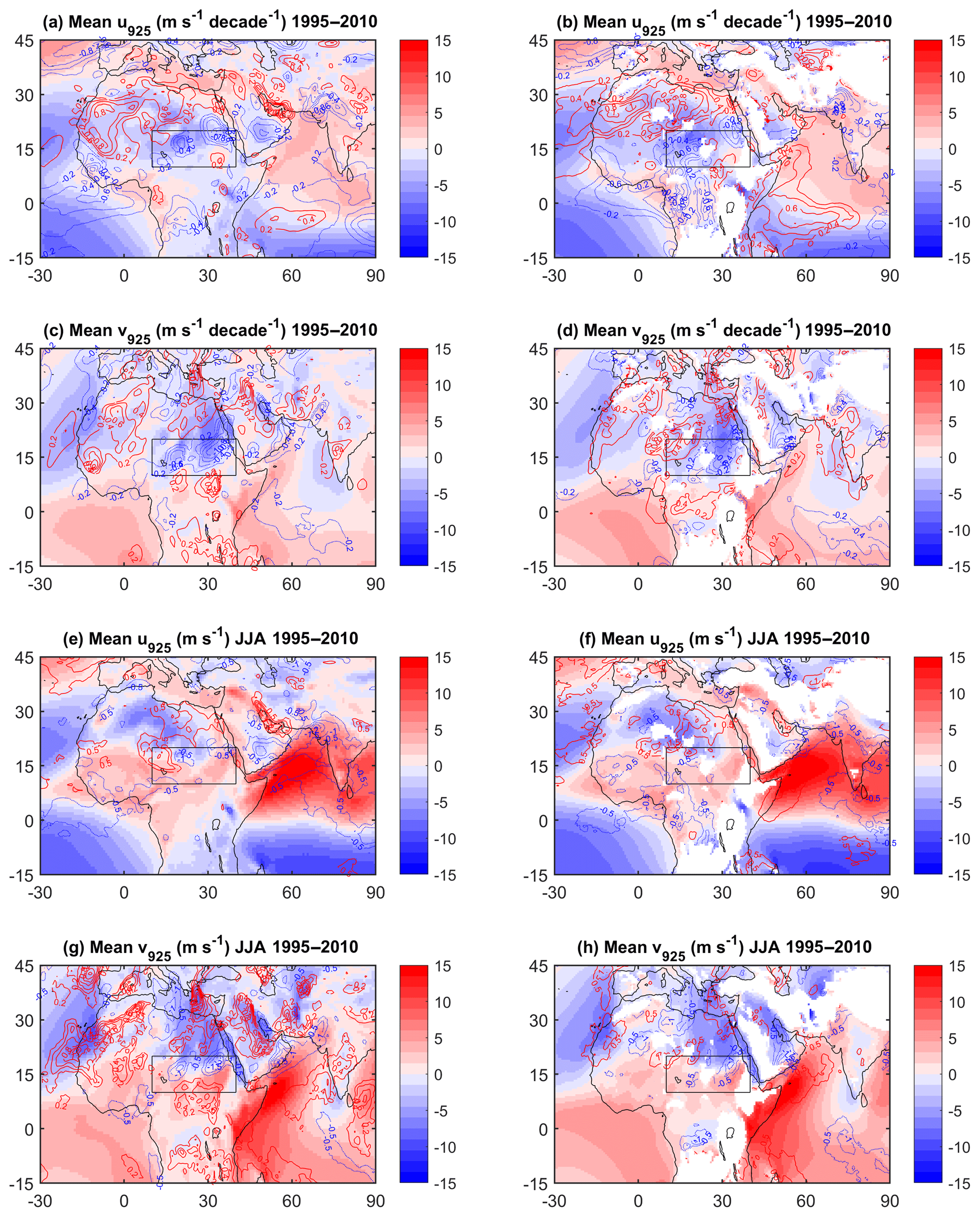
Figure 12Close-up of northern Africa showing the mean monthly and JJA fields and trends (contours) of the u and v wind components at 925 hPa (shaded). The area of focus (where IWV trends are most intense in ERA-Interim) is marked by a box.
The trend in T anomalies also stops at around 2008 (Fig. 11a). Before that period, the temperature anomaly is increasing significantly, despite strong month-to-month variability. However, there is low or negative correlation between IWV and T anomalies when considering the monthly time series. In JJA, the same periods of drying and moistening are observed (Fig. 11c). The correlation of anomalies for JJA between both reanalyses is quite good, both for IWV (around r=0.67 for the short period and r=0.63 for the longer period) and T (around r=0.69 for both periods), although their amplitudes and trends are quite different. MERRA-2 presents an overall moistening trend, while ERA-Interim shows a drying trend (Figs. 8g, h and 11c). Simultaneously, the temperature trends are both positive and significant, thus not explaining the IWV trends according to C-C.
Dynamics at 925 hPa are shown in Fig. 12. The mean states are plotted in colours over which the contours of the trends are superposed. The mean states in u925 and v925 are similar in both reanalyses, with a mean monthly north-easterly wind over the box (Fig. 12a–d) which is almost completely replaced with a south-westerly wind in JJA (Fig. 12e–h). This wind is slightly stronger in ERA-Interim than in MERRA-2. For both reanalyses, the trends in the mean flow indicate an increase in the zonal component (Fig. 12a, b). The trends in the meridional wind component show a dominant increase in the northerly wind from the Sahara. This trend may explain the general warming and drying in the eastern Sahel. The trends differ, however, with MERRA-2 showing a decrease in the northerly flow in upper-left angle of the box (Fig. 12d) while ERA-Interim shows an increase there and an increasing southerly inflow at the southern border of the box (Fig. 12c). This difference can explain the difference of intensity in these trends. In JJA, the trends in MERRA-2 are very weak (Fig. 12f, h) while in ERA-Interim there is a strong increase in the southerly flow from central Africa and in the north-easterly flow from the Sahara, explaining the net drying and warming (Fig. 11d). Figure 13 displays the inter-annual variability of JJA wind (monsoon flow) averaged over the box for both reanalyses.
It is clear that ERA-Interim has a stronger southerly flow in JJA and weaker northerly flow for the other months (Fig. 13a) with large inter-annual and decadal variability (Fig. 13b). The time series of wind in JJA in MERRA-2 clearly indicates the same four periods as for the IWV trends identified above, with a weakening of the south-westerly wind between 1980 and 1985, followed by an intensification of the monsoon flow arriving in this box between 1985 and 1995, and a wind decreasing and turning to the west until 2005 or 2006 and then becoming more stable on average. In ERA-Interim, we only observe two main periods: a weaker south–south-westerly wind at the beginning of the period followed by an intensification after 1990. The wind intensity is maximum between 1995 and 2000 but stays quite intense and with a south–south-westerly direction until the end of the period, being stronger and more southerly than in MERRA-2 after 2000. The different dynamics of the two reanalyses observed in this box partly explains the increasing deviation between both reanalyses at the end of the period.
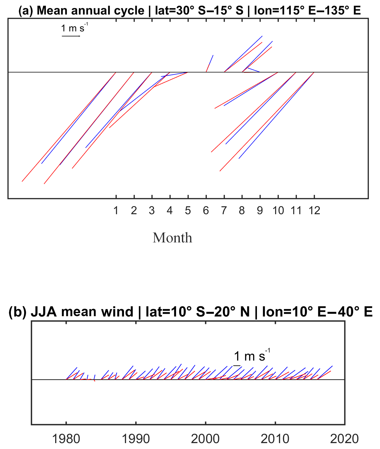
Figure 13Time series of mean wind vectors for a box over the eastern Sahel (see Fig. 12), using ERA-Interim (blue) and MERRA-2 (red) data, for the 1980 2016 period: mean annual cycle (a) and the monthly time series for the JJA season (b).
Atmospheric reanalyses play an important role in the global climate change assessment and their accuracy has significantly improved in recent years. In this study we investigated the means, variability, and trends in two modern reanalyses (ERA-Interim and MERRA-2). The means and variability in IWV in the reanalyses were inter-compared and compared to ground-based GPS data for the 1995–2010 period. ERA-Interim was shown to exhibit a slight moist bias in the extra-tropics (∼0.5 kg m−2) and a slight dry bias in the tropics in relation to both GPS and MERRA-2, which is consistent with other studies (e.g. Trenberth et al., 2011). Inter-annual variability in ERA-Interim is highly consistent with GPS, and in good agreement with MERRA-2. Differences were pointed out between GPS and reanalyses at only a few stations, mostly located in coastal regions and regions of complex topography, where representativeness errors put a limit on the comparison of gridded reanalysis data and point observations.
Previous studies have concluded that during recent decades IWV has increased with time over both land and ocean regardless of the time period and dataset analysed, except for some of the older reanalyses and/or some inhomogeneous observational datasets (Trenberth et al., 2005; Dessler and Davis, 2010; Bock et al., 2014; Schröder et al., 2016; Wang et al., 2016). Nevertheless, most global atmospheric reanalyses still have substantial limitations in representing decadal variability and trends in the water cycle components because of assimilation increments and observing system changes (Trenberth et al., 2011). In this study we found that trends in IWV and surface temperature in ERA-Interim and MERRA-2 are fairly consistent, with positive IWV trends generally correlated with surface warming over most of the tropical oceans, as well as the Arctic, part of North America, Europe, and the Amazon. However, significant differences are also found over several parts of the globe, with MERRA-2 presenting a more general global moistening trend compared to ERA-Interim. The most striking uncertainties are seen over Antarctica and most of the Southern Hemisphere, especially during JJA, where IWV trends are often of opposite signs, but also over most of central and northern Africa, as well as the Maritime Continent and central–eastern Asia. The discrepancies are observed for both the extended common time record (1980–2016) and for the shorter time period (1995–2010) when GPS data are available. Over the latter period, the GPS IWV data point to a large erroneous negative (drying) trend in ERA-Interim over Antarctica and over north-eastern Africa in JJA. The comparison with MERRA-2 indicates that both reanalyses currently have problems over northern Africa. Few in situ observations are available for assimilation in both regions and the spurious trends in ERA-Interim might be due to model biases and changes and in the assimilated satellite data (Dee et al., 2011). Further investigation using assimilation feedback statistics and satellite IWV observations would help to better understand the origin of biases and spurious trends in these regions. In most other regions, the trends in ERA-Interim have the same sign but different magnitudes than GPS, with positive biases in the tropics and negative biases in the higher northern latitudes.
The biases over Africa are likely associated with problems in representing some of the governing continental physical and dynamical processes, namely the dry convection in the Saharan heat low and moisture advections from the ocean (Meynadier et al., 2010). Variations in IWV and atmospheric circulation are strongly correlated in this arid region. This co-variability provides a reasonable explanation for the observed variability and decadal trends in each of the reanalyses and of the differences between them (e.g. stronger increase in the dry northerly flow in ERA-Interim). Here as well, assimilation feedback statistics might help to understand the origin of biases, and their link with atmospheric dynamics in this region.
A more detailed investigation of IWV, surface temperature, and atmospheric circulation was also presented for western Australia, which is in many aspects governed by similar atmospheric processes to northern Africa (dry continental convection associated with a heat low and summer monsoon). However, this region benefits from more direct in situ observations, as well as moisture and surface wind observations over the ocean from space, which have a strong impact on moisture transport from the surrounding oceans to the continent. Hence it is not surprising that both reanalyses are in better agreement and closer to the observed GPS IWV trends there. Interestingly, the region is marked by positive trends in surface temperature and IWV for the longer period, consistently with the global warming, but with an opposite IWV trend for the shorter period. The time series of IWV anomalies and surface temperature show that strong inter-annual to decadal variability in IWV is again correlated with anomalies in atmospheric circulation, with colder years being wetter.
Compared to past studies using older reanalyses, we found that modern reanalyses provide a better representation of IWV means and the strong inter-annual variability over the oceans and most continental areas. However, the weaker decadal variability and trends still suffer from large uncertainties in data-sparse regions such as Africa and Antarctica. More generally, model biases and changes in the observing system are still suspected, which prevent consistency between different reanalyses (produced with different models and assimilation systems) from being better than 10 % IWV per decade. It will be of special interest as future work to investigate ERA5, the new reanalysis from ECMWF, which benefits from many improvements compared to ERA-Interim (https://software.ecmwf.int/wiki/pages/viewpage.action?pageId=74764925, last access: October 2018).
An absolute assessment of the reanalyses was made in this study using independent IWV data from the ground-based GPS network for the period 1995–2010. Even though the GPS data were produced using homogeneous reprocessing and quality checking, inhomogeneities due to equipment changes were evidenced for a small number of sites (see Appendix B). Homogenization of the GPS dataset is currently being undertaken using different processing and modelling strategies as well as statistical homogenization techniques that should help detection and correction of the biases and offsets. An extension of the dataset is also planned as a few more years of observations are now available for reprocessing.
GPS IWV data have the following DOI: global GPS IWV data at 120 stations of IGS permanent network, https://doi.org/10.14768/06337394-73a9-407c-9997-0e380dac5591 (Bock, 2016). ERA-Interim data can be downloaded at https://www.ecmwf.int/en/forecasts/datasets/archive-datasets/reanalysis-datasets/era-interim (last access: October 2018; Dee et al., 2011). MERRA-2 data can be downloaded at https://gmao.gsfc.nasa.gov/reanalysis/MERRA-2/ (last access: October 2018; Gelaro et al., 2017). The results presented in the paper are also provided in the Supplement.
There are many methods used in the literature to estimate linear trends from geophysical data. Two of the most widely used are compared in this Appendix, the Theil–Sen method (after Theil, 1950; Sen, 1968), which we used in the paper, and the least squares method (e.g. Weatherhead et al., 1998). Both methods assume that the data time series, yi, can be modelled by a linear function of time ti of the following form:
where a and b are the unknown slope and intercept parameters to be estimated, and Ni is the random noise or error. The ordinary least squares method determines the set of parameters (, ) that minimizes the sum of squared residuals:
The Theil–Sen method, as defined by Theil (1950), is a non-parametric method that determines the trend by computing the median of slopes of lines through all pairs of points in the time series:
and once the slope has been estimated, the intercept is derived from . Sen (1968) extended the method to handle the case when two data points have the same time (so-called ties).
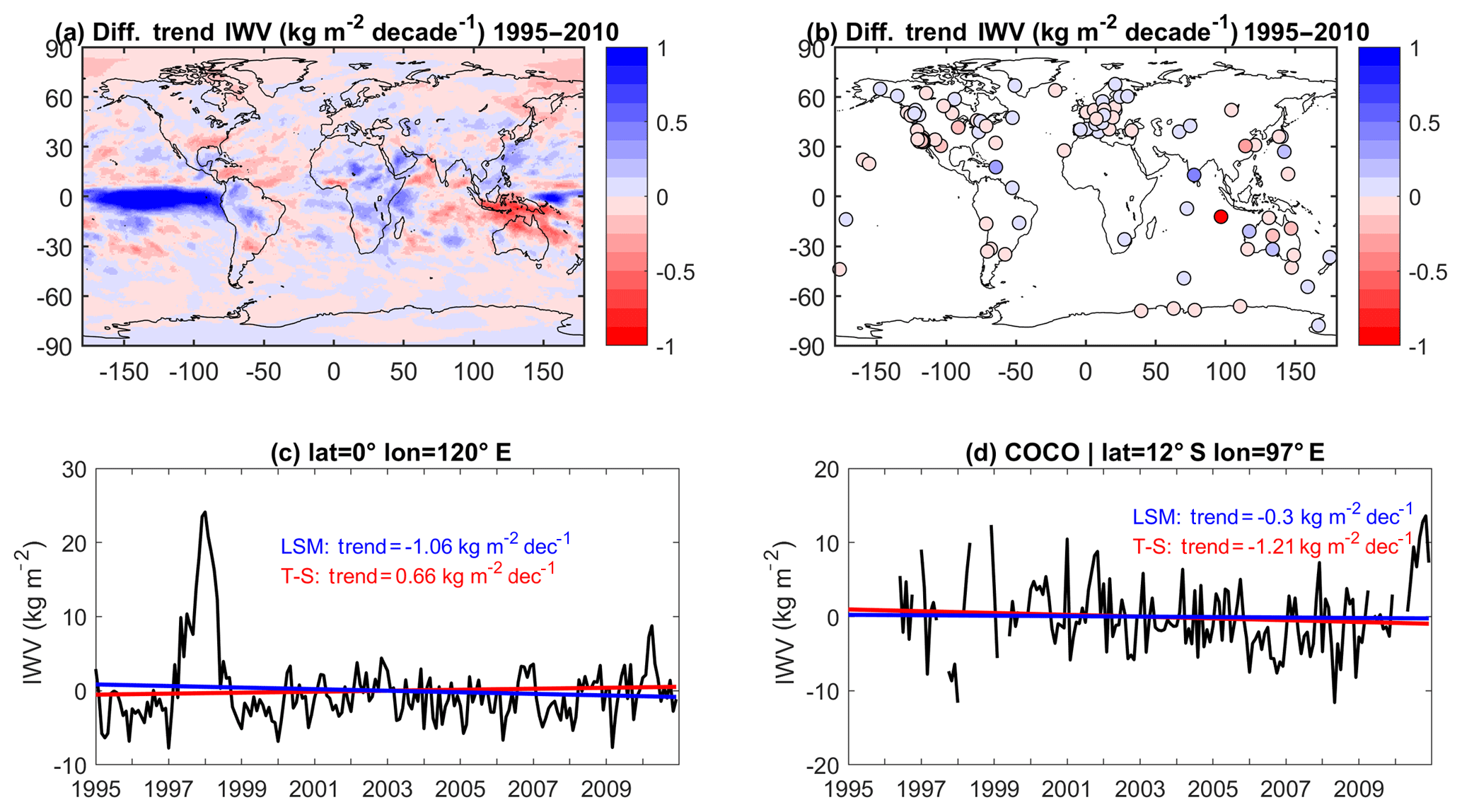
Figure A1(a) Trend differences between two methods of computing trends (Theil–Sen minus the least squares method) for the ERA-Interim data used in the paper. The root mean square of the difference is 0.20 kg m−2 decade−1. (b) Same as panel (a), but for the GPS data at 104 stations. The root mean square of the difference is 0.14 kg m−2 decade−1. (c) Time series of IWV anomaly in ERA-Interim at a point of large difference between methods in the tropical Pacific ocean with superposed linear trends. (d) Time series of IWV anomaly at the COCO GPS site with superposed linear trends.
We compared both methods, which were applied to the global ERA-Interim and GPS monthly mean IWV anomalies, for the 1995–2010 period. The results are shown in Fig. A1. The differences between trends obtained using the two methods for the ERAI data are below 0.5 kg m−2 decade−1 for most of the globe, except around the Equator, where the ordinary least squares method overestimates the trends in the eastern Pacific Ocean and underestimates the trends in the western Pacific Ocean (Fig. A1a) with respect to the Theil–Sen method. Consistent results are observed from the GPS IWV anomalies including gaps in the times series as shown in Fig. A1b.
The time series and trends at two points over the regions with large opposite differences are shown in Fig. A1c (eastern Pacific Ocean) and Fig. A1d (Coco Island in the western Pacific Ocean). It is observed that the Theil–Sen method is less affected by the strong positive anomalies observed in 1997–1998 in the tropical Pacific (due to a strong El Niño event), and at the end of the time series, in 2010, for the Coco Island GPS station. In fact, the Theil–Sen estimator is known to be generally more robust than the least squares method (Rousseeuw and Leroy, 2003) and less sensible to the beginning and ending of the time series (Wang et al., 2016), so this was the method chosen to estimate the trends analysed throughout the paper.
B1 Data and methods
The GPS and reanalyses do not agree at certain GPS sites. In this appendix we discuss in more detail the various causes for this, and especially those that originate from problems in the GPS data. In order to minimize the representativeness differences between the gridded reanalysis fields and the GPS point observations, a more elaborate intercomparison methodology is required. We used the ERA-Interim 6-hourly pressure level data (37 levels between 1000 and 1 hPa, among which 27 levels lie between 1000 and 100 hPa) from the four grid points surrounding each GPS station. For each grid point and time step, the IWV is recomputed by vertically integrating the specific humidity from the height of the GPS station to the top of the atmosphere (1 hPa). Most GPS station heights fall between two pressure levels, and the specific humidity at the station height can be interpolated from the adjacent levels. The reanalysis data are only extrapolated for stations located at pressure values over 1000 hPa (the lowest pressure level). Interpolation and extrapolation are done linearly for specific humidity and temperature, and exponentially for pressure. The IWV at the location of the GPS stations is then obtained by a bilinear interpolation from the four IWV estimates. This approach provided more consistent reanalysis IWV estimates by comparison with the GPS data than any other approach that we tested (the GPS–reanalysis differences are diminished at almost all sites, with a few exceptions). The use of 6-hourly fields also allows time-matching of the GPS data before computing monthly averages, reducing temporal sampling issues.
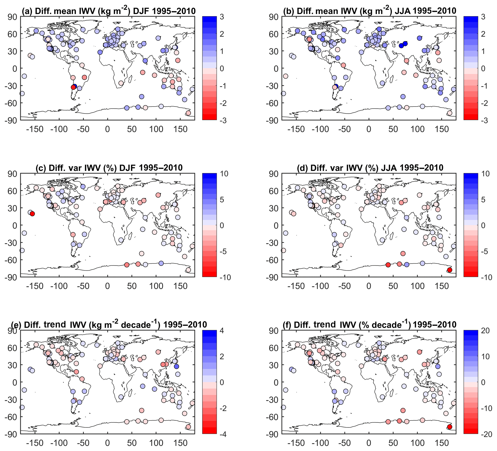
Figure B1(a) Difference of mean IWV estimates (ERA-Interim minus GPS) for DJF 1995–2010 from time-matched IWV series, (b) same as panel (a) for JJA, (c) difference of relative variability estimates (ERA-Interim variability minus GPS variability) for DJF 1995–2010 from time-matched IWV series, (d) same as panel (c) for JJA, (e) difference of trend estimates (ERA-Interim minus GPS) for 1995–2010 from time-matched IWV series, (f) same as panel (e) for relative trends.

Figure B2Time series of IWV from GPS (black) and ERAI (red), and IWV difference (blue) at stations (a) CFAG, (b) KIT3, (c) MCM4, (d) SYOG, (e) CCJM, and (f) WUHN. Filled circles show DJF values and open circles JJA values. Crosses show individual months used in both seasons. Vertical dashed lines indicate GPS equipment changes (receiver in magenta, antenna in green) and GPS processing changes (in orange). Note the change in vertical scales between figures.
B2 Differences in the means and in inter-annual variability
The mean IWV differences between ERA-Interim and GPS are shown in Fig. B1a and b for all 104 GPS sites. At first glance, the results look very similar to those presented in Fig. 4a and b using a simplified comparison methodology.
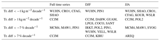
Table B1Stations with most intense trend differences (ERAI − GPS) computed from time-matched GPS and ERA-Interim IWV series.
The sites with most notable differences in the IWV means (ERA-Interim minus GPS) are CFAG in the Andes cordillera with a bias of 6.5 kg m−2 (27 %) in DJF and 3.9 kg m−2 (43 %) in JJA, SANT in Chile with −2.4 kg m−2 (−15 %) in DJF, and TSKB (in Japan) with 1.9 kg m−2 (24 %) in DJF. In JJA, four other sites have large biases: KIT3 in Uzbekistan with a value of 6.2 kg m−2 (35 %), POL2 in Kyrgyzstan with 3.2 kg m−2 (20 %), SYOG in Antarctica with 0.6 kg m−2 (32 %), and MAW1 in Antarctica with 0.4 kg m−2 (31 %). The inspection of the time series shows that at some of these stations the biases are not constant in time but contain large seasonal variations, such as at CFAG (Fig. B2a) or KIT3 (Fig. B2b) for example. These sites are located in coastal regions and/or regions with complex topography. Although we used here a more elaborate spatial and temporal matching of reanalysis and GPS data, representativeness errors can still be the cause of these biases. To investigate this point, we compared the (vertically adjusted) IWV values from all four grid points surrounding each GPS station to the bilinearly interpolated IWV value. We found that at CFAG, KIT3, POL2, SYOG, and MAW1, the bilinearly interpolated values did not minimize the IWV biases between the reanalysis and GPS. At these sites, the altitudes of the four grid points differ by more than 500 m and the moisture profiles above are very different. In the case of SANT, although the interpolated value matches the GPS value better than any of the four surrounding grid point values, there is still a large bias explained by a variation in the altitude of the grid points of over 1500 m.
Figure B1c and d show the differences of relative standard deviations between ERA-Interim and GPS. In JJA, the four stations with the largest differences (ERAI − GPS) are located in Antarctica: MCM4, SYOG, MAW1, and DAV1 with differences of −39.7 % (p=0), −7.5 % (p=0.14), −4.6 % (p=0.21), and +4.1 % (p=0.17), respectively. In DJF, the largest differences are found for MKEA (Hawaii) and SYOG, where they amount to −11.5 % (p=0.33) and −4.7 % (p=0.13), respectively. In the case of SYOG, MAW1, and DAV1, representativeness errors are suspected again because of the large variability in the IWV values of the surrounding grid points connected with large variations in the altitudes (> 500 m) of these grid points. In the case of MKEA, the variation in the altitude of the surrounding grid points is quite small because of the limited imprint of Mauna Kea Island on the 0.75∘ resolution grid of ERA-Interim. However, the difference in altitude between the GPS station and all four grid points is larger than 3000 m. In the case of MCM4 and SYOG, the inspection of the time series of monthly mean IWV and IWV differences (shown in Fig. B2c and d) reveals variations in the means which coincide with GPS equipment changes and processing changes and unexplained variations in the amplitude of the seasonal cycle, resulting in a marked oscillation in the monthly mean differences (ERAI − GPS). Variations in the means introduce a spurious component of variability in the GPS IWV series (e.g. in JJA, at MCM4 the standard deviation of GPS IWV is 56.9 % compared to 17.2 % for ERAI).
B3 Differences in trends
Inspection of Fig. 4a found a number of GPS stations where the trend estimates are large and of opposite sign compared to ERA-Interim: CCJM (south of the Japanese home islands), DARW (northern Australia), WUHN (eastern China), IRKT (central Russia), ANKR (Turkey), KOKB and MKEA (Hawaii), and MCM4 (Antarctica). Some of them (DARW, ANKR, KOKB, MKEA) are located in areas where the ERA-Interim trends change sign and a perfect spatial coincidence between the reanalysis and observations might not be expected. On the other hand, stations CCJM, WUHN, IRKT, and MCM4 are located within regions where the ERA-Interim trends are strong and significant and extend over large areas. For some of these stations, the discrepancy is due to gaps and/or inhomogeneities in the GPS time series which corrupt the trend estimates.
Figure B1e and f show the trend differences for the time-matched series. Compared to Fig. 4, the agreement is improved at DARW, ANKR, and IRKT, and at many other sites (e.g. KELY in Greenland, SANT, MAW1). However, there are still many sites with large differences. The stations with largest differences are listed in Table B1.
Inspection of time series reveals the presence of large inhomogeneities at CCJM, MCM4 (see Fig. B2c), WUHN, SHAO, and CRO1. At CCJM (see Fig. B2e), the GPS–ERA-Interim IWV difference time series has a large offset in 2001 which coincides with a GPS equipment change (receiver and antenna). This offset is responsible for a large negative trend estimate in the GPS series (−1.40 kg m−2 decade−1), whereas the time-matched ERA-Interim series gives a positive trend (+0.98 kg m−2 decade−1), consistent with the large-scale trend in the reanalysis seen in Fig. 4. At WUHN (Fig. B2f), the GPS trend estimate is positive (0.34 kg m−2 decade−1) while the ERA-Interim estimate is negative (−1.45 kg m−2 decade−1). The IWV difference time series shows several breaks (in 1999, 2005, and at the end of 2006) though none of them coincides with known GPS equipment changes. In fact, the break at the end of 2006 is associated with the change in radiosonde from the Shang-M to Shang-E, which is assimilated by ERA-Interim (Wang and Zhang, 2008). Zhao et al. (2012) found that prior to this change there was a 2 kg m−2 wet bias in the radiosonde data at the Wuhan station, in comparison with GPS. This moist bias is also observed in ERA-Interim prior to the end of 2006. At SHAO and CRO1 and a few other sites (e.g. SYOG, DARW, ANKR), inhomogeneity in the IWV difference series coincides with documented GPS equipment changes (not shown). Representativeness differences are also suspected at some mountainous and coastal sites (e.g. AREQ, CFAG, KIT3, MAW1, SANT, SYOG, and the other sites discussed in the previous section), while some sites also show more gradual drifts in the times series which do not seem connected with known GPS equipment changes (e.g. MAW1, Antarctica). At such sites, drifts in the reanalysis are plausible. Overall, the seasonal trends estimated from the GPS data confirm the trends found in ERA-Interim. The sites with largest differences in the seasonal estimates are also listed in Table B1. In addition to the sites where issues were noticed in the monthly trends, the list includes a few more sites which are also visible in Fig. 5a and b (most notably KIRU in Sweden, COCO in the Indian Ocean, IRKT in Russia, and ANKR in Turkey). Trend estimates at some of these sites might be inaccurate due to the enhanced impact of time gaps for the short seasonal time series (based on 16 years at best).
The supplement related to this article is available online at: https://doi.org/10.5194/acp-18-16213-2018-supplement.
ACP performed the data analysis (computation of means, variability and trends) and wrote the paper. OB prepared the GPS IWV data and contributed to the data analysis and writing of the paper. SB contributed to the data analysis and writing of the paper.
The authors declare that they have no conflict of interest.
This article is part of the special issue “Advanced Global Navigation Satellite Systems tropospheric products for monitoring severe weather events and climate (GNSS4SWEC) (AMT/ACP/ANGEO inter-journal SI)”. It is not associated with a conference.
This work was developed in the framework of the VEGA
project and supported by the CNRS program LEFE/INSU and ANR REMEMBER project
(grant ANR-12-SENV-001). This work is a contribution to the European COST
Action ES1206 GNSS4SWEC (GNSS for Severe Weather and Climate monitoring;
http://www.cost.eu/COST_Actions/essem/ES1206, last access: October 2018) aiming for the
development of the global GPS network for atmospheric research and climate
change monitoring.
Edited by: Roeland Van Malderen
Reviewed by: three anonymous referees
Bauer, P.: 4D-Var assimilation of MERIS total column water-vapour retrievals over land, Q. J. Roy. Meteor. Soc., 135, 1852–1862, https://doi.org/10.1002/qj.509, 2009.
Bock, O.: GPS data: Daily and monthly reprocessed IWV data from 120 global GPS stations, version 1.2, https://doi.org/10.14768/06337394-73a9-407c-9997-0e380dac5591, 2016.
Bock, O., Keil, C., Richard, E., Flamant, C., and Bouin, M. N.: Validation of precipitable water from ECMWF model analyses with GPS and radiosonde data during the MAP SOP, Q. J. Roy. Meteor. Soc., 131, 3013–3036, 2005.
Bock, O., Bouin, M. N., Walpersdorf, A., Lafore, J. P., Janicot, S., and Guichard, F.: Comparison of GPS precipitable water vapour to independent observations and Numerical Weather Prediction model reanalyses over Africa, Q. J. Roy. Meteor. Soc., 133, 2011–2027, https://doi.org/10.1002/qj.185, 2007.
Bock, O., Willis, P., Wang, J., and Mears, C.: A high-quality, homogenized, global, long-term (1993–2008) DORIS precipitable water data set for climate monitoring and model verification, J. Geophys. Res.-Atmos., 119, 7209–7230, https://doi.org/10.1002/2013JD021124, 2014.
Bock, O., Bosser, P., Pacione, R., Nuret, M., Fourrié, N., and Parracho, A.: A high-quality reprocessed ground-based GPS dataset for atmospheric process studies, radiosonde and model evaluation, and reanalysis of HyMeX Special Observing Period, Q. J. Roy. Meteor. Soc., 142, 56–71, https://doi.org/10.1002/qj.2701, 2016.
Bosilovich, M. G., Robertson, F. R., Takacs, L., Molod, A., and Mocko, D.: Atmospheric Water Balance and Variability in the MERRA-2 Reanalysis. J. Climate, 30, 1177–1196, https://doi.org/10.1175/JCLI-D-16-0338.1, 2017.
Brown, J. R., Moise, A. F., Colman, R., and Zhang, H.: Will a Warmer World Mean a Wetter or Drier Australian Monsoon?, J. Climate, 29, 4577–4596, https://doi.org/10.1175/JCLI-D-15-0695.1, 2016.
Byun, S. H. and Bar-Server, Y. E.: A new type of troposphere zenith path delay product of the international GNSS service, J. Geodesy, 83, 367–373, https://doi.org/10.1007/s00190-008-0288-8, 2009.
Chen, B. and Liu, Z.: Global water vapor variability and trend from the latest 36 year (1979 to 2014) data of ECMWF and NCEP reanalyses, radiosonde, GPS, and microwave satellite, J. Geophys. Res.-Atmos., 121, 11442–11462, https://doi.org/10.1002/2016JD024917, 2016.
Dee, D. P. and Uppala, S.: Variational bias correction of satellite radiance data in the ERA-Interim reanalysis, Q. J. Roy. Meteor. Soc., 135, 1830–1841, https://doi.org/10.1002/qj.493, 2009.
Dee, D. P., Uppala, S. M., Simmons, A. J., Berrisford, P., Poli, P., Kobayashi, S., Andrae, U., Balmaseda, M. A., Balsamo, G., Bauer, P., and Bechtold, P.: The ERA-Interim reanalysis: Configuration and performance of the data assimilation system, Q. J. Roy. Meteor. Soc., 137, 553–597, https://doi.org/10.1002/qj.828, 2011.
Dessler, A. E. and Davis, S. M.: Trends in tropospheric humidity from reanalysis systems, J. Geophys. Res.-Atmos., 115, D19127, https://doi.org/10.1029/2010JD014192, 2010.
Gelaro, R., McCarty, W., Suárez, M. J., Todling, R., Molod, A., Takacs, L., Randles, C. A., Darmenov, A., Bosilovich, M. G., Reichle, R., and Wargan, K.: The modern-era retrospective analysis for research and applications, version 2 (MERRA-2), J. Climate, 30, 5419–5454, https://doi.org/10.1175/JCLI-D-16-0758.1, 2017.
Grose, M. R., Brown, J. N., Narsey, S., Brown, J. R., Murphy, B. F., Langlais, C., Gupta, A. S., Moise, A. F., and Irving, D. B.: Assessment of the CMIP5 global climate model simulations of the western tropical Pacific climate system and comparison to CMIP3, Int. J. Climatol., 34, 3382–3399, https://doi.org/10.1002/joc.3916, 2014
Hamed, K. H. and Rao, A. R.: A modified Mann-Kendall trend test for autocorrelated data, J. Hydrol., 204, 182–196, https://doi.org/10.1016/S0022-1694(97)00125-X, 1998.
Held, I. M. and Soden, B. J.: Robust responses of the hydrological cycle to global warming, J. Climate, 19, 5686–5699, https://doi.org/10.1175/JCLI3990.1, 2006.
Hendon, H. H., Thompson, D. W. J., Wheeler, and M. C.: Australian Rainfall and Surface Temperature Variations Associated with the Southern Hemisphere Annular Mode, J. Climate, 20, 2452–2467, https://doi.org/10.1175/JCLI4134.1, 2007.
IGSMAIL-6298: Reprocessed IGS Trop Product now available with Gradients, by Yoaz Bar-Sever, 11 November 2012, available at: https://lists.igs.org/pipermail/igsmail/2010/000132.html (last access: October 2018), 2012.
Karbou, F., Rabier, F., Lafore, J.-P., Redelsperger, J. L., and Bock, O.: Global 4D-Var assimilation and forecast experiments using land surface emissivities from AMSU-A and AMSU-B. Part-II: Impact of adding surface channels on the African Monsoon during AMMA, Weather Forecast., 25, 20–36, https://doi.org/10.1175/2009WAF2222244.1, 2010.
Kondratev, K. Y.: Radiation Processes in the Atmosphere, World Meteorological Organization, Geneva, Switzerland, 1972.
Lorenc, A. C.: Analysis methods for numerical weather prediction, Q. J. Roy. Meteor. Soc., 112, 1177–1194, https://doi.org/10.1002/qj.49711247414, 1986.
Mears, C. A., Wang, J., Smith, D., and Wentz, F. J.: Intercomparison of total precipitable water measurements made by satellite-borne microwave radiometers and ground-based GPS instruments, J. Geophys. Res.-Atmos., 120, 2492–2504, https://doi.org/10.1002/2014JD022694, 2015.
Meynadier, R., Bock, O., Gervois, S., Guichard, F., Redelsperger, J.-L., Agustí-Panareda, A., and Beljaars, A.: West African Monsoon water cycle: 2. Assessment of numerical weather prediction water budgets, J. Geophys. Res., 115, D19107, https://doi.org/10.1029/2010JD013919, 2010.
Mieruch, S., Schröder, M., Noël, S., and Schulz, J.: Comparison of decadal global water vapour changes derived from independent satellite time series, J. Geophys. Res.-Atmos., 119, 12489–12499, https://doi.org/10.1002/2014JD021588, 2014.
Ning, T., Wickert, J., Deng, Z., Heise, S., Dick, G., Vey, S., and Schöne, T.: Homogenized time series of the atmospheric water vapour content obtained from the GNSS reprocessed data, J. Climate, 29, 2443–2456, https://doi.org/10.1175/JCLI-D-15-0158.1, 2016.
O'Gorman, P. A. and Muller, C. J.: How closely do changes in surface and column water vapor follow Clausius–Clapeyron scaling in climate-change simulations?, Environ. Res. Lett., 5, 025207, https://doi.org/10.1088/1748-9326/5/2/025207, 2010.
Power, S., Tseitkin, F., Torok, S., Lavery, B., and McAvaney, B.: Australian temperature, Australian rainfall, and the Southern Oscillation, 1910–1996: Coherent variability and recent changes, Aust. Meteorol. Mag., 47, 85–101, 1998.
Robertson, F. R., Bosilovich, M. G., Roberts, J. B., Reichle, R. H., Adler, R., Ricciardulli, L., Berg, W., and Huffman, G. J.: Consistency of Estimated Global Water Cycle Variations over the Satellite Era, J. Climate, 27, 6135–6154, https://doi.org/10.1175/JCLI-D-13-00384.1, 2014.
Rousseeuw, P. J. and Leroy, A. M.: Robust Regression and Outlier Detection, Wiley Series in Probability and Mathematical Statistics, 516, Wiley, USA, p. 67, 2003.
Sanogo, S., Fink, A. H., Omotosho, J. A., Ba, A., Redl, R., and Ermert, V.: Spatio-temporal characteristics of the recent rainfall recovery in West Africa, Int. J. Climatol., 35, 4589–4605, https://doi.org/10.1002/joc.4309, 2015.
Schneider, T., O'Gorman, P. A., and Levine, X. J.: Water vapor and the dynamics of climate changes, Rev. Geophys., 48, RG3001, https://doi.org/10.1029/2009RG000302, 2010.
Schröder, M., Lockhoff, M., Forsythe, J. M., Cronk, H. Q., Vonder Haar, T. H., and Bennartz, R.: The GEWEX Water Vapour Assessment: Results from Intercomparison, Trend, and Homogeneity Analysis of Total Column Water Vapour, J. Appl. Meteorol. Clim., 55, 1633–1649, https://doi.org/10.1175/JAMC-D-15-0304.1, 2016.
Sen, P. K.: Estimates of the regression coefficient based on Kendall's tau, J. Am. Stat. Assoc., 63, 1379–1389, https://doi.org/10.2307/2285891, 1968.
Sherwood, S. C., Roca, R., Weckwerth, T. M., and Andronova, N. G.: Tropospheric water vapor, convection, and climate, Rev. Geophys., 48, RG2001, https://doi.org/10.1029/2009RG000301, 2010.
Theil, H.: A rank-invariant method of linear and polynomial regression analysis, I, II, III, Nederl. Akad. Wetensch., Proc., 53, 386–392, 521–525, 1397–1412, https://doi.org/10.1007/978-94-011-2546-8_20, 1950.
Thorne, P. W. and Vose, R. S.: Reanalyses Suitable for Characterizing Long-Term Trends, B. Am. Meteorol. Soc., 91, 353–362, https://doi.org/10.1175/2009BAMS2858.1, 2010.
Trenberth, K. E., Fasullo, J., and Smith, L.: Trends and variability in column-integrated atmospheric water vapour, Clim. Dynam., 24, 741–758, https://doi.org/10.1007/s00382-005-0017-4, 2005.
Trenberth, K. E., Fasullo, J. T., and Mackaro, J.: Atmospheric Moisture Transports from Ocean to Land and Global Energy Flows in Reanalyses, J. Climate, 24, 4907–4924, https://doi.org/10.1175/2011JCLI4171.1, 2011.
Vey, S., Dietrich, R., Fritsche, M., Rülke, A., Steigenberger, P., and Rothacher, M.: On the homogeneity and interpretation of precipitable water time series derived from global GPS observations, J. Geophys. Res.-Atmos., 114, D10101, https://doi.org/10.1029/2008JD010415, 2009.
Wang, J. and Zhang, L.: Systematic errors in global radiosonde precipitable water data from comparisons with ground-based GPS measurements, J. Climate, 21, 2218–2238, https://doi.org/10.1175/2007JCLI1944.1, 2008.
Wang, J., Zhang, L., and Dai, A.: Global estimates of water-vapour-weighted mean temperature of the atmosphere for GPS applications, J. Geophys. Res., 110, D21101, https://doi.org/10.1029/2005JD006215, 2005.
Wang, J., Dai, A., and Mears, C.: Global Water Vapour Trend from 1988 to 2011 and Its Diurnal Asymmetry Based on GPS, Radiosonde, and Microwave Satellite Measurements, J. Climate, 29, 5205–5222, https://doi.org/10.1175/JCLI-D-15-0485.1, 2016.
Weatherhead, E. C., Reinsel, G. C., Tiao, G. C., Meng, X. L., Choi, D., Cheang, W. K., Keller, T., DeLuisi, J., Wuebbles, D. J., Kerr, J. B., Miller, A. J., Oltmans, S. J., and Frederick, J. E.: Factors affecting the detection of trends: Statistical considerations and applications to environmental data, J. Geophys. Res.-Atmos., 103, 17149–17161, https://doi.org/10.1029/98JD00995, 1998.
Zhao, T., Dai, A., and Wang, J.: Trends in tropospheric humidity from 1970 to 2008 over China from a homogenized radiosonde dataset J. Climate, 25, 4549–4567, https://doi.org/10.1175/JCLI-D-11-00557.1, 2012.
- Abstract
- Introduction
- Datasets and methods
- Comparison between GPS and reanalyses IWV (1995–2010)
- Long-term IWV trends in the reanalyses (1980–2016)
- Summary and conclusions
- Data availability
- Appendix A: Comparison between methods of trend estimation
- Appendix B: Detailed comparison between ERA-Interim and GPS at the GPS sites
- Author contributions
- Competing interests
- Special issue statement
- Acknowledgements
- References
- Supplement